Identifying unknown source in degenerate parabolic equation from final observation

Abstract

In this article, for a degenerate parabolic equation we study an inverse problem for restoration of source temperature from the information of final temperature profile. The uniqueness of this inverse problem is first established by taking an integral transform and using Liouville's theorem (complex analysis). With aids of an integral identity, a Lipschitz stability for the inverse problem is further constructed. Finally, several numerical experiments are presented to show the accuracy and efficiency of the algorithm.

Keywords:

• Degenerate parabolic equation
• inverse source problem
• final observation
• uniqueness
• stability

2010 Mathematics Subject Classifications:

• 35K65
• 35R30
• 35B53

1. Introduction and main results

Throughout this paper, assuming T is a given positive number and ρ is known as a $C^1[0,T]$-function, we study a one-dimensional parabolic equation degenerating at the boundary of the space domain, namely (1) ${\mathrm{\partial }}_{t}u-{\mathrm{\partial }}_x\left(a\right(x\left){\mathrm{\partial }}_{x}u\right)=\rho \left(t\right)f\left(x\right),(x,t)\in (0,1)\times (0,T)$(1) with suitable boundary condition which will be given later. We suppose that the degenerate coefficient $a(\cdot )$ satisfies the following conditions: (2) $a\in C[0,1]\cap C^1(0,1],a\left(x\right)>0\mathrm{i}\mathrm{n}(0,1]\mathrm{a}\mathrm{n}\mathrm{d}a\left(0\right)=0.$(2) The study of such degenerate parabolic equation was initially motivated by some physical and financial mathematics models. For example, in the heat transfer, the thermal conductivity coefficient $a\left(x\right)$ is usually related to the structure of the material, density and other factors. The lower the value of $a\left(x\right)$, the stronger its heat resistance. So if the value of $a\left(x\right)$ on the boundary x = 0 is so small, then the model (1(1) ${\mathrm{\partial }}_{t}u-{\mathrm{\partial }}_x\left(a\right(x\left){\mathrm{\partial }}_{x}u\right)=\rho \left(t\right)f\left(x\right),(x,t)\in (0,1)\times (0,T)$(1) ) can be regarded as an approximation of this case, which indicates the ability to resist heat transfer. We refer to e.g. Buchot and Raymond [1], Martinez et al. [14], Oleinik and Samokhin [15] for motivating examples of a Crocco-type equation coming from the study of the velocity field of a laminar flow on a flat plate. The well known Black–Scholes equation is such the case where the degenerate parabolic boundary degeneracy occurs at the boundary (see e.g. Egger and Engl [8] and Jiang and Tao [12]).

In Equation (1(1) ${\mathrm{\partial }}_{t}u-{\mathrm{\partial }}_x\left(a\right(x\left){\mathrm{\partial }}_{x}u\right)=\rho \left(t\right)f\left(x\right),(x,t)\in (0,1)\times (0,T)$(1) ), the term $\rho \left(t\right)f\left(x\right)$ is called the source term and it is crucial to know or determine the coefficient f. However, usually this term cannot be directly measured due to the mixing of the effects of several factors, which requires one to use inverse problems to identify these quantities by involving additional information that can be observed or measured practically. In this paper, our main concern is:

Problem 1.1

Consider the degenerate parabolic equation (1(1) ${\mathrm{\partial }}_{t}u-{\mathrm{\partial }}_x\left(a\right(x\left){\mathrm{\partial }}_{x}u\right)=\rho \left(t\right)f\left(x\right),(x,t)\in (0,1)\times (0,T)$(1) ) with the following initial condition (3) $u(x,0)=0,x\in (0,1)$(3) and boundary condition (4) $\begin{array}{rl}& u(0,t)=0,\text{if }{a}^{-1}\in L^1(0,1),\\ & \underset{x\to 0+}{lim}a\left(x\right)u_x(x,t)=0,\text{if }{a}^{-\frac{1}{2}}\in L^1(0,1),\\ & u(1,t)=0,t\in (0,T).\end{array}$(4) Determine the unknown source f from the final state observation $u(x,T)$, $x\in (0,1)$.

Problems of this type have important applications in several fields of applied science and engineering. For example, f usually describes the medium properties of generating heat source or heat sink in thermology. For recovering the source term, sometimes we have to measure the final state of the solution u since it is difficult to obtain the information of the solution at the early stage of the diffusion processes.

As is known, inverse source problems for classical parabolic equations are well studied in the literature. Here we do not intend to give a complete list of references, and one can consult Choulli and Yamamoto [5], Hasanov and Slodi$\check{c}$ka [10], Isakov [11] and Rundell and Colton [16] for example. However, to the best of the authors' knowledge, the works concerned with inverse degenerate problems are quite few in contrast with the non-degenerate case. In Cannarsa et al. [4], the Carleman estimate with singular weight function was established for (1(1) ${\mathrm{\partial }}_{t}u-{\mathrm{\partial }}_x\left(a\right(x\left){\mathrm{\partial }}_{x}u\right)=\rho \left(t\right)f\left(x\right),(x,t)\in (0,1)\times (0,T)$(1) ) with $a\left(x\right)=x^{\alpha }$ $(0<\alpha <2)$, from which an inverse source problem with addition boundary data was discussed. Similarly, we refer to Tort [18] where the Lipschitz stability results in inverse source problems for the degenerate parabolic equations was established by the global Carleman estimates. We refer to Deng et al. [6] and Rao et al. [20] for theoretical and numerical treatments on determining the source term in (1(1) ${\mathrm{\partial }}_{t}u-{\mathrm{\partial }}_x\left(a\right(x\left){\mathrm{\partial }}_{x}u\right)=\rho \left(t\right)f\left(x\right),(x,t)\in (0,1)\times (0,T)$(1) ). [6] reconstructed the source by a numerical algorithm on the basis of the conjugate gradient method. In [20], an iteration scheme of the Landweber type is applied to handle the numerical solution of the inverse problem. We also refer to Deng and Yang [7] and Tort and Vancostenoble [19] for the coefficient inverse problems, and refer to Yang and Deng [21] for the backward problem for the degenerate parabolic equation. For other topics of degenerate parabolic equations, e.g. the null controllability, we may refer the reader to Cannarsa et al. [2,3] and the references therein.

In this paper, for the degenerate parabolic equation (1(1) ${\mathrm{\partial }}_{t}u-{\mathrm{\partial }}_x\left(a\right(x\left){\mathrm{\partial }}_{x}u\right)=\rho \left(t\right)f\left(x\right),(x,t)\in (0,1)\times (0,T)$(1) ), we show that in the case where ρ is only t-dependent and smooth enough, the spatial component can be uniquely determined from the final overdetermination. We have

Theorem 1.1

Assume $\rho \in C^1[0,T]$ is positive for any $t\in [0,T]$. Let $f\in L^2(0,1)$ and suppose u solves Equation (1(1) ${\mathrm{\partial }}_{t}u-{\mathrm{\partial }}_x\left(a\right(x\left){\mathrm{\partial }}_{x}u\right)=\rho \left(t\right)f\left(x\right),(x,t)\in (0,1)\times (0,T)$(1) ) with initial-boundary conditions (3(3) $u(x,0)=0,x\in (0,1)$(3) ) and (4(4) $\begin{array}{rl}& u(0,t)=0,\text{if }{a}^{-1}\in L^1(0,1),\\ & \underset{x\to 0+}{lim}a\left(x\right)u_x(x,t)=0,\text{if }{a}^{-\frac{1}{2}}\in L^1(0,1),\\ & u(1,t)=0,t\in (0,T).\end{array}$(4) ). Then $u(\cdot ,T)\equiv 0$ in $(0,1)$ implies $f\equiv 0$ in $(0,1)$.

By the above theorem, we can further see that when the data have some perturbations, the source term must have corresponding changes.

Theorem 1.2

Under the same assumptions in Theorem 1.1, we suppose that $(u_i,f_i)$, i = 1, 2 are two pairs of solutions of our inverse source problem correspondingly to data $h_i:=u_i(x,T),$ i = 1, 2. Then $\parallel f_1-f_2{\parallel }_{\mathcal{B}}\le \parallel h_1-h_2{\parallel }_{L^2(0,1)}.$

Here the norm $\parallel \cdot {\parallel }_{\mathcal{B}}$ will be given in Section 3.

For proving Theorem 1.1, several technical lemmas for this degenerate parabolic equation are needed, so we collect them in Sections 2.1 and 2.2. Preparing all necessities, say, Lemmas 2.2 and 2.3, by Liouville's theorem (complex analysis) we will finish the proof of Theorem 1.1 in Section 2. In the following Section 3, an integral identity is to be put forward with which the stability in Theorem 1.2 can be constructed via a suitable topology. In Section 4, an iteration thresholding method based on the Tikhonov regularization is designed to obtain the numerical solution for our inverse source problem, and some typical numerical experiments are tested to be verified the validity of the iteration scheme. Finally, concluding remarks are given in Section 5.

2. Proof of Theorem 1.1

In this section, we will set up notations and terminologies, review some of standard facts on the functional analysis and give the proof of Theorem 1.1.

2.1. Weighted Sobolev spaces and Hardy inequality

In this part, we introduce a weighted Sobolev spaces and a Hardy-type inequality which play an important role in the proof of our inverse source problem as well as the regularity estimates for the solution to Equation (1(1) ${\mathrm{\partial }}_{t}u-{\mathrm{\partial }}_x\left(a\right(x\left){\mathrm{\partial }}_{x}u\right)=\rho \left(t\right)f\left(x\right),(x,t)\in (0,1)\times (0,T)$(1) ) with the initial-boundary conditions (3(3) $u(x,0)=0,x\in (0,1)$(3) ) and (4(4) $\begin{array}{rl}& u(0,t)=0,\text{if }{a}^{-1}\in L^1(0,1),\\ & \underset{x\to 0+}{lim}a\left(x\right)u_x(x,t)=0,\text{if }{a}^{-\frac{1}{2}}\in L^1(0,1),\\ & u(1,t)=0,t\in (0,T).\end{array}$(4) ).

In addition to (2(2) $a\in C[0,1]\cap C^1(0,1],a\left(x\right)>0\mathrm{i}\mathrm{n}(0,1]\mathrm{a}\mathrm{n}\mathrm{d}a\left(0\right)=0.$(2) ), we suppose that the degenerate coefficient $a(\cdot )$ satisfies the following conditions:

• $\mathrm{\exists }\alpha \in (0,2)$ such that $x{a}^{\prime }\left(x\right)\le \alpha a\left(x\right)$ for every $x\in (0,1]$.

• If $\alpha \in [1,2)$, there exist m>0 and ${\delta }_0>0$ such that for every $x\in [0,{\delta }_0]$, we have $a\left(x\right)\ge m\underset{0\le y\le x}{sup}a\left(y\right).$

For example, $a\left(x\right)=x^{\alpha }$ satisfies the above conditions. Under these assumptions on the degenerate coefficient $a(\cdot )$, the boundary condition (4(4) $\begin{array}{rl}& u(0,t)=0,\text{if }{a}^{-1}\in L^1(0,1),\\ & \underset{x\to 0+}{lim}a\left(x\right)u_x(x,t)=0,\text{if }{a}^{-\frac{1}{2}}\in L^1(0,1),\\ & u(1,t)=0,t\in (0,T).\end{array}$(4) ) can be rephrased as follows: (5) $\begin{array}{rl}& u(0,t)=0,\text{if }0<\alpha <1,\\ & a\left(0\right)u_x(0,t)=0,\text{if }1\le \alpha <2,\\ & u(1,t)=0,t\in (0,T).\end{array}$(5)

Remark 2.1

We point out that the functional framework in which the problem is well posed depends on whether $0<\alpha <1$ or $1\le \alpha <2$. We distinguish the two following cases: I. $0<\alpha <1$, the weakly degenerate case at 0; II. $1\le \alpha <2$, the strongly degenerate case at 0.

We introduce the following weighted Sobolev space related to the degenerate coefficient $a(\cdot )$: $H_a^1(0,1)=\left\{u\in L^2(0,1)\cap H_{\mathrm{l}\mathrm{o}\mathrm{c}}^1(0,1];{\int }_0^{1}a\left(x\right)|u_x\left(x\right){|}^2\mathrm{d}x<+\mathrm{\infty }\right\}$ which is a Hilbert space with the scalar product $\mathrm{\forall }u,v\in H_a^1(0,1),(u,v)={\int }_0^{1}uv+a\left(x\right)u_x{v}_x\mathrm{d}x.$ We define the unbounded operator A : $D\left(A\right)\subset L^2(0,1)\to L^2(0,1)$ by $\mathrm{\forall }u\in D\left(A\right),Au:={\mathrm{\partial }}_x\left(a\right(x\left){\mathrm{\partial }}_{x}u\right),$ where $D\left(A\right)$ will be given later.

Definition 2.1

Weak degeneracy

For $\alpha \in (0,1)$, we define (6) $H_{a,0}^1(0,1):=\left\{u\in H_a^1(0,1);u\left(0\right)=u\left(1\right)=0\right\},$(6) and we let (7) $D\left(A\right):=\left\{u\in H_{a,0}^1(0,1)\cap H_{\mathrm{l}\mathrm{o}\mathrm{c}}^1(0,1];(a{u}_x{)}_x\in L^2(0,1)\right\}.$(7)

Definition 2.2

Strong degeneracy

For $\alpha \in [1,2)$, we let (8) $H_{a,0}^1(0,1):=\left\{u\in H_a^1(0,1);u\left(1\right)=0\right\}.$(8) We define $D\left(A\right)$ as follows (9) $D\left(A\right):=\left\{u\in H_{a,0}^1(0,1)\cap H_{\mathrm{l}\mathrm{o}\mathrm{c}}^1(0,1];(a{u}_x{)}_x\in L^2(0,1),\underset{x\to 0+}{lim}a{u}_x=0\right\}.$(9)

Thus, in the case of $\alpha \in (0,1)$, if $u\in D\left(A\right)$, then u satisfies the Dirichlet boundary condition $u\left(0\right)=u\left(1\right)=0$ and in the case $\alpha \in [1,2)$, every $u\in D\left(A\right)$ satisfies the Neumann boundary condition $\underset{x\to 0+}{lim}\left(a{u}_x\right)\left(x\right)=0$ and the Dirichlet boundary condition $u\left(1\right)=0$. Moreover, the operator A is the infinitesimal generator of a strongly continuous semigroup $e^{tA}$ on $L^2(0,1)$. Consequently, we have the following well-posedness result (see, e.g. Futouhi and Salimi [9, Theorem 14]).

Proposition 2.1

Let ρ be given in $L^2(0,T)$ and $f\in L^2(0,1)$. For all $\alpha \in [0,2),$ Equation (1(1) ${\mathrm{\partial }}_{t}u-{\mathrm{\partial }}_x\left(a\right(x\left){\mathrm{\partial }}_{x}u\right)=\rho \left(t\right)f\left(x\right),(x,t)\in (0,1)\times (0,T)$(1) ) with the initial-boundary conditions (3(3) $u(x,0)=0,x\in (0,1)$(3) ) and (5(5) $\begin{array}{rl}& u(0,t)=0,\text{if }0<\alpha <1,\\ & a\left(0\right)u_x(0,t)=0,\text{if }1\le \alpha <2,\\ & u(1,t)=0,t\in (0,T).\end{array}$(5) ) has a unique solution $u\in C\left(\right[0,T];L^2(0,1\left)\right)\cap L^2(0,T;H_a^1(0,1\left)\right)$.

Moreover, we have the following Hardy-type inequality of the solution in the framework of weighted Sobolev spaces $H_a(0,1)$.

Lemma 2.1

Hardy-type inequality, e.g. [9, Remark 20]

Let $\alpha \in (0,2),$ we have ${\int }_0^{1}a\left(x\right)u_x^2\mathrm{d}x\ge C{\int }_0^1{u}^2\mathrm{d}x,\mathrm{\forall }u\in H_{a,0}^1(0,1),$ where the constant C>0 depending only on $a\left(1\right)$ and α.

2.2. Estimates under frequency domain

In this part, we will show several useful lemmas which are mainly concerned with the estimates of the solution of Equation (1(1) ${\mathrm{\partial }}_{t}u-{\mathrm{\partial }}_x\left(a\right(x\left){\mathrm{\partial }}_{x}u\right)=\rho \left(t\right)f\left(x\right),(x,t)\in (0,1)\times (0,T)$(1) ) with initial-boundary conditions (3(3) $u(x,0)=0,x\in (0,1)$(3) ) and (5(5) $\begin{array}{rl}& u(0,t)=0,\text{if }0<\alpha <1,\\ & a\left(0\right)u_x(0,t)=0,\text{if }1\le \alpha <2,\\ & u(1,t)=0,t\in (0,T).\end{array}$(5) ) under frequency domain. For this, we multiply both sides of Equation in (1(1) ${\mathrm{\partial }}_{t}u-{\mathrm{\partial }}_x\left(a\right(x\left){\mathrm{\partial }}_{x}u\right)=\rho \left(t\right)f\left(x\right),(x,t)\in (0,1)\times (0,T)$(1) ) by $e^{-st}$ with $s\in \mathbb{C}$, and integrate from 0 to T to derive ${\int }_0^T{\mathrm{\partial }}_{t}u\left(t\right)e^{-st}\mathrm{d}t-{\int }_0^{T}Au\left(t\right)e^{-st}\mathrm{d}t=f\left(x\right){\int }_0^T\rho \left(t\right)e^{-st}\mathrm{d}t.$ Noting that $u\left(0\right)=0$, from integration by parts, we find (10) $-A\hat{u}\left(s\right)+s\hat{u}\left(s\right)=f\left(x\right)\hat{\rho }\left(s\right)-u(x,T)e^{-sT},s\in \mathbb{C},$(10) where (11) $\hat{u}\left(s\right):={\int }_0^{T}u\left(t\right)e^{-st}\mathrm{d}t,\hat{\rho }\left(s\right):={\int }_0^T\rho \left(t\right)e^{-st}\mathrm{d}t.$(11)

Lemma 2.2

Let $\epsilon >0$ and $\delta >0$ be a sufficiently small and fixed constants. Assuming the function $\rho \in C^1[0,T]$ is positive in $[0,T]$. Then there exists a positive constant $C=C({\rho }_0:=\underset{[0,T]}{inf}\rho ,\epsilon ,\delta ,T)$ such that the following inequality $|\hat{\rho }\left(s\right)|=\left|{\int }_0^T\rho \left(t\right)e^{-st}\mathrm{d}t\right|\ge C{\int }_0^T{e}^{-t\mathrm{\Re }s}\mathrm{d}t$ is valid for any $s\in \{\mathrm{\Re }s\le -\epsilon ;|\mathrm{\Im }s|\le \delta \}$.

Proof.

We will prove the above inequality holds true in either of the following two cases.

Case 1  $s\in \{\mathrm{\Re }s\le -K;|\mathrm{\Im }s|\le \delta \}$.

Case 2  $s\in \{-K\le \mathrm{\Re }s\le -\epsilon ;|\mathrm{\Im }s|\le \delta \}$.

In Case 1, by integration by parts we represent $\hat{\rho }\left(s\right)$ as follows ${\int }_0^T\rho \left(t\right)e^{-st}\mathrm{d}t=\frac{\rho \left(0\right)-\rho \left(T\right)e^{-sT}}{s}+s^{-1}{\int }_0^T{\rho }^{\prime }\left(t\right)e^{-st}\mathrm{d}t=:I_1\left(s\right)+I_2\left(s\right).$ For $I_2\left(s\right)$, by a direct calculation, we find $|I_2\left(s\right)|\le |s{|}^{-1}{\int }_0^T|{\rho }^{\prime }\left(t\right)|e^{-t\mathrm{\Re }s}\mathrm{d}t\le \frac{\parallel \rho {\parallel }_{C^1[0,T]}}{|s|}\frac{1-e^{-T\mathrm{\Re }s}}{\mathrm{\Re }s}.$ The choice of s, say, $\mathrm{\Re }s\le -\epsilon$ implies that (12) $\frac{1-e^{-T\mathrm{\Re }s}}{\mathrm{\Re }s}\le \frac{e^{T|\mathrm{\Re }s|}}{|\mathrm{\Re }s|},$(12) which can be further used to derive that $|I_2\left(s\right)|\le \frac{\parallel \rho {\parallel }_{C^1[0,T]}{e}^{T|\mathrm{\Re }s|}}{|\mathrm{\Re }s||s|}.$ Let us turn to evaluating $I_1\left(s\right)$. For this, a direct calculation derives $s{I}_1\left(s\right)=\rho \left(0\right)-\rho \left(T\right)e^{-T\mathrm{\Re }s}\cos \left(T\mathrm{\Im }s\right)+i\rho \left(T\right)e^{-T\mathrm{\Re }s}\sin \left(T\mathrm{\Im }s\right),$ hence that $|s{I}_1\left(s\right){|}^2=\rho (T{)}^2{e}^{-2T\mathrm{\Re }s}-2\rho (0\left)\rho \right(T)e^{-T\mathrm{\Re }s}\cos (T\mathrm{\Im }s)+\rho (0{)}^2,$ finally that $|I_1\left(s\right){|}^2=\frac{{\left(\rho \left(T\right)e^{-T\mathrm{\Re }s}-\rho \left(0\right)\right)}^2}{|s{|}^2}+2\rho \left(0\right)\rho \left(T\right)e^{-T\mathrm{\Re }s}\frac{1-\cos \left(T\mathrm{\Im }s\right)}{|s{|}^2}.$ Moreover, by the inequality $\frac{|1-\cos t|}{t^2}\le C$, $t\in \mathbb{R}$, we see that $\frac{|1-\cos \left(T\mathrm{\Im }s\right)|}{|s{|}^2}=\frac{|1-\cos \left(T\mathrm{\Im }s\right)|}{|T\mathrm{\Im }s{|}^2}\frac{|T\mathrm{\Im }s{|}^2}{|s{|}^2}\le C{T}^2,s\in \mathbb{C}.$ Combining all the above estimates, we find $|I_1\left(s\right){|}^2\ge \frac{{\left(\rho \left(T\right)e^{-T\mathrm{\Re }s}-\rho \left(0\right)\right)}^2}{|s{|}^2}-2C{T}^2\rho \left(0\right)\rho \left(T\right)e^{-T\mathrm{\Re }s}.$ Now for sufficiently large $|s|$, then $|\mathrm{\Re }s|$ is also sufficiently large in view of (12(12) $\frac{1-e^{-T\mathrm{\Re }s}}{\mathrm{\Re }s}\le \frac{e^{T|\mathrm{\Re }s|}}{|\mathrm{\Re }s|},$(12) ). Consequently there exists a constant $C=C(K,T,\rho )$ such the estimate $|I_1\left(s\right)|\ge \frac{C{e}^{-T\mathrm{\Re }s}}{|s|}$ provided that $\mathrm{\Re }s<-K$ with K>0 is a sufficiently large constant.

Finally, in Case 1, that is, $s\in \{\mathrm{\Re }s\le -K\}$ with sufficiently large K>0, we have $\left|{\int }_0^T\rho \left(t\right)e^{-st}\mathrm{d}t\right|\ge |I_1\left(s\right)|-|I_2\left(s\right)|\ge \frac{e^{T|\mathrm{\Re }s|}}{|s|}\left(C-\frac{\parallel \rho {\parallel }_{C^1[0,T]}}{|\mathrm{\Re }s|}\right)\ge \frac{C{e}^{T|\mathrm{\Re }s|}}{2|s|}.$ Moreover, noting that $|\mathrm{\Im }s|\le \delta \le K$ implies $|s{|}^2\le 2|\mathrm{\Re }s{|}^2$, we further see that ${\int }_0^T{e}^{-t\mathrm{\Re }s}\mathrm{d}t\le \frac{e^{T|\mathrm{\Re }s|}}{|\mathrm{\Re }s|}\le \sqrt{2}\frac{e^{T|\mathrm{\Re }s|}}{|s|},$ which derives that $\left|{\int }_0^T\rho \left(t\right)e^{-st}\mathrm{d}t\right|\ge C{\int }_0^T{e}^{-t\mathrm{\Re }s}\mathrm{d}t\text{in Case 1.}$ Next, we evaluate $\hat{\rho }\left(s\right)$ in Case 2, that is, the case when s lies in $\{s\in \mathbb{C};-K\le \mathrm{\Re }s\le -\epsilon ;|\mathrm{\Im }s|\le \delta \}$. By taking δ small enough, we are led to $|\sin \left(t\mathrm{\Im }s\right)|\le |t\mathrm{\Im }s|\le \frac{1}{4},\cos \left(t\mathrm{\Im }s\right)\ge \frac{1}{2}.$ We first rewrite $\hat{\rho }\left(s\right)$ as follows $\hat{\rho }\left(s\right)={\int }_0^T\rho \left(t\right)e^{-t\mathrm{\Re }s}\cos \left(t\mathrm{\Im }s\right)\mathrm{d}t+i{\int }_0^T\rho \left(t\right)e^{-t\mathrm{\Re }s}\sin \left(t\mathrm{\Im }s\right)\mathrm{d}t,$ hence that $|\hat{\rho }\left(s\right)|\ge \frac{1}{2}{\int }_0^T\rho \left(t\right)e^{t|\mathrm{\Re }s|}\mathrm{d}t-\frac{1}{4}{\int }_0^T\rho \left(t\right)e^{t|\mathrm{\Re }s|}\mathrm{d}t\ge \frac{{\rho }_0}{4}{\int }_0^T{e}^{t|\mathrm{\Re }s|}\mathrm{d}t=\frac{{\rho }_0(e^{T|\mathrm{\Re }s|}-1)}{4|\mathrm{\Re }s|},$ where ${\rho }_0:=\underset{t\in [0,T]}{inf}\rho \left(t\right)>0$. Finally, we obtain $|\hat{\rho }\left(s\right)|\ge C\frac{e^{T|\mathrm{\Re }s|}-1}{|\mathrm{\Re }s|}>C_1>0,s\in \{s\in \mathbb{C};-K\le \mathrm{\Re }s\le -\epsilon ;|\mathrm{\Im }s|\le \delta \},$ where the constant $C_1>0$ is only dependent on $T,\rho ,\epsilon ,\delta$. Moreover, for $-K\le \mathrm{\Re }s\le -\epsilon$, one can easily check that ${\int }_0^T{e}^{-t\mathrm{\Re }s}\mathrm{d}t\le T{e}^{KT},$ therefore, we have $\left|{\int }_0^T\rho \left(t\right)e^{-st}\mathrm{d}t\right|\ge C{\int }_0^T{e}^{-t\mathrm{\Re }s}\mathrm{d}t\text{in Case 2.}$ Collecting all the above estimates we finish the proof of the lemma.

Lemma 2.3

Assume $\rho \in C^1[0,T]$ is positive for any $t\in [0,T]$. Let $f\in L^2(0,1)$ and suppose u solves Equation (1(1) ${\mathrm{\partial }}_{t}u-{\mathrm{\partial }}_x\left(a\right(x\left){\mathrm{\partial }}_{x}u\right)=\rho \left(t\right)f\left(x\right),(x,t)\in (0,1)\times (0,T)$(1) ) with initial-boundary conditions (3(3) $u(x,0)=0,x\in (0,1)$(3) ) and (4(4) $\begin{array}{rl}& u(0,t)=0,\text{if }{a}^{-1}\in L^1(0,1),\\ & \underset{x\to 0+}{lim}a\left(x\right)u_x(x,t)=0,\text{if }{a}^{-\frac{1}{2}}\in L^1(0,1),\\ & u(1,t)=0,t\in (0,T).\end{array}$(4) ). Then the function $\hat{u}:\mathbb{C}\to D\left(A\right)$ which is defined in (11(11) $\hat{u}\left(s\right):={\int }_0^{T}u\left(t\right)e^{-st}\mathrm{d}t,\hat{\rho }\left(s\right):={\int }_0^T\rho \left(t\right)e^{-st}\mathrm{d}t.$(11) ) can be estimated as follows (13) $\parallel \hat{u}\left(s\right){\parallel }_{L^2(0,1)}\le C|\hat{\rho }\left(s\right)|\parallel f{\parallel }_{L^2(0,1)},s\in \mathbb{C}.$(13)

Proof.

We denote $\overline{\hat{u}}\left(s\right)$ as the conjugate of the complex valued function $\hat{u}\left(s\right)$. Then multiplying $\overline{\hat{u}}\left(s\right)$ on both sides of Equation (10(10) $-A\hat{u}\left(s\right)+s\hat{u}\left(s\right)=f\left(x\right)\hat{\rho }\left(s\right)-u(x,T)e^{-sT},s\in \mathbb{C},$(10) ), and taking integral on $(0,1)$ lead to ${\int }_0^1(-A\hat{u}(s\left)\right)\overline{\hat{u}}\left(s\right)+s\hat{u}\left(s\right)\overline{\hat{u}}\left(s\right)\mathrm{d}x=\hat{\rho }\left(s\right){\int }_0^1\overline{\hat{u}}\left(s\right)f\left(x\right)\mathrm{d}x-e^{-sT}{\int }_0^{1}u\left(T\right)\overline{\hat{u}}\left(s\right)\mathrm{d}x,s\in \mathbb{C}.$ Here we omitted the x in $\hat{u}(x,s)$ and $u(x,T)$ when no confusion can arise. Integration by parts yields $B_s\left[\hat{u}\right(s),\hat{u}(s\left)\right]=\rho \left(s\right){\int }_0^1\hat{f}\left(x\right)\overline{\hat{u}}\left(s\right)\mathrm{d}x-e^{-sT}{\int }_0^{1}u\left(T\right)\overline{\hat{u}}\left(s\right)\mathrm{d}x,$ where $B_s\left[\hat{u}\right(s),\hat{u}(s\left)\right]:={\int }_0^{1}a\left(x\right){\hat{u}}_x\left(s\right)\overline{{\hat{u}}_x\left(s\right)}+s|\hat{u}\left(s\right){|}^2\mathrm{d}x.$ The real part of $B_s[\hat{u},\hat{u}]$ can be represented as follows: (14) $\mathrm{\Re }\left(B_s[\hat{u},\hat{u}]\right)={\int }_0^{1}a\left(x\right)|{\hat{u}}_x{|}^2+\mathrm{\Re }s|\hat{u}\left(s\right){|}^2\mathrm{d}x,$(14) while the imaginary part is (15) $\mathrm{\Im }{B}_s[\hat{u},\hat{u}]={\int }_0^1\mathrm{\Im }s|\hat{u}\left(s\right){|}^2\mathrm{d}x.$(15) Now in the case of $\mathrm{\Re }s\ge -\epsilon$, where $\epsilon >0$ will be chosen later, we find from (14(14) $\mathrm{\Re }\left(B_s[\hat{u},\hat{u}]\right)={\int }_0^{1}a\left(x\right)|{\hat{u}}_x{|}^2+\mathrm{\Re }s|\hat{u}\left(s\right){|}^2\mathrm{d}x,$(14) ) that ${\int }_0^{1}a\left(x\right)|{\hat{u}}_x\left(s\right){|}^2+\mathrm{\Re }s|\hat{u}\left(s\right){|}^2\mathrm{d}x\le |B_s[\hat{u},\hat{u}]|,$ which combined with Lemma 2.1 yields ${\int }_0^{1}C|\hat{u}\left(s\right){|}^2+\mathrm{\Re }s|\hat{u}\left(s\right){|}^2\mathrm{d}x\le |\hat{\rho }\left(s\right)|{\int }_0^1|f\left(x\right)||\hat{u}\left(s\right)|\mathrm{d}x+|e^{-sT}|{\int }_0^1|u\left(T\right)||\hat{u}\left(s\right)|\mathrm{d}x.$ By the Hölder inequality, we have $\begin{array}{rl}& {\int }_0^{1}C|\hat{u}\left(s\right){|}^2+\mathrm{\Re }s|\hat{u}\left(s\right){|}^2\mathrm{d}x\\ & \le |\hat{\rho }\left(s\right)|{\left[{\int }_0^1{f}^2\left(x\right)\mathrm{d}x\right]}^{\frac{1}{2}}{\left[{\int }_0^1|\hat{u}\left(s\right){|}^2\mathrm{d}x\right]}^{\frac{1}{2}}\\ & +|e^{-sT}|{\left[{\int }_0^1{u}^2\left(T\right)\mathrm{d}x\right]}^{\frac{1}{2}}{\left[{\int }_0^1|\hat{u}\left(s\right){|}^2\mathrm{d}x\right]}^{\frac{1}{2}},\end{array}$ therefore $(\mathrm{\Re }s+C){\left[{\int }_0^1|\hat{u}\left(s\right){|}^2\mathrm{d}x\right]}^{\frac{1}{2}}\le |\hat{\rho }\left(s\right)|{\left[{\int }_0^1{f}^2\left(x\right)\mathrm{d}x\right]}^{\frac{1}{2}}+|e^{-sT}|{\left[{\int }_0^1{u}^2\left(T\right)\mathrm{d}x\right]}^{\frac{1}{2}},$ that is, $(\mathrm{\Re }s+C)\parallel \hat{u}\left(s\right){\parallel }_{L^2(0,1)}\le |\hat{\rho }\left(s\right)|\parallel f{\parallel }_{L^2(0,1)}+|e^{-sT}|\parallel u\left(T\right){\parallel }_{L^2(0,1)}.$ Now we choose ϵ being small enough so that $C-\epsilon >\frac{C}{2}$, then $\parallel \hat{u}\left(s\right){\parallel }_{L^2(0,1)}\le C|\hat{\rho }\left(s\right)|\parallel f{\parallel }_{L^2(0,1)}+C|e^{-sT}|\parallel u\left(T\right){\parallel }_{L^2(0,1)}.$ Let us turn to the case of $s\in \{\mathrm{\Re }s\le -\epsilon ;|\mathrm{\Im }s|\le \delta \}$, from the definition of $\hat{u}\left(s\right)$, it follows that $\parallel \hat{u}\left(s\right){\parallel }_{L^2(0,1)}\le {\int }_0^T\parallel u\left(t\right){\parallel }_{L^2(0,1)}{e}^{-t\mathrm{\Re }s}\mathrm{d}t\le C\parallel f{\parallel }_{L^2(0,1)}{\int }_0^T{e}^{-t\mathrm{\Re }s}\mathrm{d}t.$ Then Lemma 2.2 derives $\parallel \hat{u}\left(s\right){\parallel }_{L^2(0,1)}\le C\parallel f{\parallel }_{L^2(0,1)}|\hat{\rho }\left(s\right)|.$ It remains to consider the case of $s\in \{\mathrm{\Re }s\le -\epsilon ;|\mathrm{\Im }s|\ge \delta \}$, where $\delta >0$ is sufficiently small. In view of (15(15) $\mathrm{\Im }{B}_s[\hat{u},\hat{u}]={\int }_0^1\mathrm{\Im }s|\hat{u}\left(s\right){|}^2\mathrm{d}x.$(15) ), we see that $\begin{array}{rl}& |\mathrm{\Im }s|{\int }_0^1|\hat{u}\left(s\right){|}^2\mathrm{d}x\\ & \le |\hat{\rho }\left(s\right)|{\left({\int }_0^1{f}^2\left(x\right)\mathrm{d}x\right)}^{\frac{1}{2}}{\left({\int }_0^1|\hat{u}\left(s\right){|}^2\mathrm{d}x\right)}^{\frac{1}{2}}\\ & +|e^{-sT}|{\left[{\int }_0^1{u}^2\left(T\right)\mathrm{d}x\right]}^{\frac{1}{2}}{\left[{\int }_0^1|\hat{u}\left(s\right){|}^2\mathrm{d}x\right]}^{\frac{1}{2}}.\end{array}$ Then $\begin{array}{rl}\parallel \hat{u}\left(s\right){\parallel }_{L^2(0,1)}& \le \frac{C}{|\mathrm{\Im }s|}\left(|\hat{\rho }\left(s\right)|\parallel f{\parallel }_{L^2(0,1)}+|e^{-sT}|\parallel u\left(T\right){\parallel }_{L^2(0,1)}\right)\\ & \le C\left(|\hat{\rho }\left(s\right)|\parallel f{\parallel }_{L^2(0,1)}+|e^{-sT}|\parallel u\left(T\right){\parallel }_{L^2(0,1)}\right).\end{array}$

2.3. Proof of Theorem 1.1

As a direct application of the estimates in the above subsection, we will give a proof of Theorem 1.1.

Proof

Proof of Theorem 1.1

Since $\hat{u}\left(s\right)$ and $\hat{\rho }\left(s\right)$ are analytic in $\mathbb{C}$, and hence $F_{\varphi }\left(s\right):=\frac{{\int }_0^1\hat{u}\left(s\right)\varphi \left(x\right)\mathrm{d}x}{\hat{\rho }\left(s\right)}$ is a holomorphic function in $\mathbb{C}$ removing the zero points of $\hat{\rho }\left(s\right)$, where $\varphi \in L^2(0,1)$ is arbitrarily fixed. However, from hyperthesis $u\left(T\right)=0$, Lemma 2.3 and Riemann's theorem (see, e.g. [17]) guarantee that all the singularities of the function $F_{\varphi }\left(s\right)$ are removable, and then this function can be regarded as an analytic function in $\mathbb{C}$ and is bounded on $\mathbb{C}$. Thus the Liouville theorem (see, e.g. [17]) implies that the analytic function $F_{\varphi }\left(s\right)$ must be independent of s, that is, there exists a constant $C_{\varphi }$ depending on ϕ such that $F_{\varphi }\left(s\right)=C_{\varphi }$, $\mathrm{\forall }s\in \mathbb{C}$.

Now we take the parameter s be real number and we claim that $C_{\varphi }$ must be zero by letting $s\to +\mathrm{\infty }$ in $F_{\varphi }\left(s\right)$. Indeed, by integration by parts, we find that $s\hat{\rho }\left(s\right)=\rho \left(0\right)-\rho \left(T\right)e^{-sT}+{\int }_0^T{\rho }^{\prime }\left(t\right)e^{-st}\mathrm{d}t\to \rho \left(0\right),\mathrm{a}\mathrm{s}s\to +\mathrm{\infty }.$ We estimate the part ${\int }_0^1\hat{u}(x;s)\varphi \left(x\right)\mathrm{d}x$, s>0, as follows $\begin{array}{rl}\left|{\int }_0^1\hat{u}(x;s)\varphi \left(x\right)\mathrm{d}x\right|& \le {\int }_0^{\delta }\left|{\int }_0^{1}u(x,t)\varphi \left(x\right)\mathrm{d}x{e}^{-st}\mathrm{d}t\right|\\ & +{\int }_{\delta }^T\left|{\int }_0^{1}u(x,t)\varphi \left(x\right)\mathrm{d}x{e}^{-st}\mathrm{d}t\right|=I_1+I_2.\end{array}$ Here $0<\delta <T$ will be chosen in the following. From Proposition 2.1, we see that for any $\epsilon >0$, there exists $\delta >0$ such that $|{\int }_0^{1}u(x,t)\varphi \left(x\right)\mathrm{d}x|<\epsilon$ for any $|x|<\delta$. Therefore, $I_1\le \epsilon {\int }_0^{\delta }{e}^{-st}\mathrm{d}t\le \frac{\epsilon }{s}(1-e^{-s\delta }),s>0.$ It remains to evaluate $I_2$. By noting $u\in C\left(\right[0,T];L^2(0,1\left)\right)$, a direct calculation yields $I_2\le \parallel u{\parallel }_{C\left(\right[0,T];L^2(0,1\left)\right)}\parallel \varphi {\parallel }_{L^2(0,1)}{\int }_{\delta }^T{e}^{-st}\mathrm{d}t\le C\parallel u{\parallel }_{C\left(\right[0,T];L^2(0,1\left)\right)}\parallel \varphi {\parallel }_{L^2(0,1)}\frac{e^{-s\delta }-e^{-sT}}{s}.$ Collecting all the above estimates, we finally obtain $\left|{\int }_0^{1}s\hat{u}(x;s)\varphi \left(x\right)\mathrm{d}x\right|\le \epsilon (1-e^{-s\delta })+C\parallel u{\parallel }_{C\left(\right[0,T];L^2(0,1\left)\right)}\parallel \varphi {\parallel }_{L^2(0,1)}(e^{-s\delta }-e^{sT}),$ which implies ${\overline{lim}}_{s\to +\mathrm{\infty }}\left|{\int }_0^{1}s\hat{u}(x;s)\varphi \left(x\right)\mathrm{d}x\right|\le \epsilon .$ We must have $\underset{s\to +\mathrm{\infty }}{lim}\left|{\int }_0^{1}s\hat{u}(x;s)\varphi \left(x\right)\mathrm{d}x\right|=0$ since $\epsilon >0$ can be arbitrarily small.

Since $C_{\varphi }$ is independent of s, these two estimates for $s\hat{u}\left(s\right)$ and $s\hat{\rho }\left(s\right)$ imply that the constant $C_{\varphi }$ is zero, which further implies $\hat{u}(x;s)\equiv 0$, $x\in (0,1),s\in \mathbb{C}$ by noting $\varphi \in L^2(0,1)$ can be arbitrarily chosen. Consequently ${\int }_0^{\mathrm{\infty }}\tilde{u}\left(t\right)e^{-st}\mathrm{d}t=0,s\in \mathbb{C},$ where $\tilde{u}\left(t\right):=u\left(t\right)$ if $t\in (0,T)$ and $\tilde{u}$ vanishes outside of $(0,T)$, which implies $u(x,t)\equiv 0$ in $(0,1)\times (0,T)$ due to the uniqueness of the Laplace transform, and hence $f\equiv 0$ in $(0,1)$. We complete the proof of the theorem.

Remark 2.2

Here we should mention that this kind of inverse source problem in the non-degenerate cases has been well studied thanks to the eigensystem of the elliptic operator. We do not know if the Fourier expansion can also perform well in dealing with our case. In fact, the traditional eigenfunction expansion argument requires the symmetry of the equation, and also the nonsingular coefficients are needed. However, our method based on the integral transform has no special requirements for the structure of the equation, except that the coefficient must be time independent.

3. Proof of Theorem 1.2

In this section, following the arguments used in Li and Yamamoto [13], a Lipschitz stability for determining the source magnitude will be established.

3.1. An integral identity

For proving the second main result, we will give an integral identity with aid of an adjoint problem, which reflects a corresponding relation of varied of the unknown source functions with changes of the initial-boundary values and additional observations.

Lemma 3.1

Consider $u_j,$ $j=1,2,$ the solution of (1(1) ${\mathrm{\partial }}_{t}u-{\mathrm{\partial }}_x\left(a\right(x\left){\mathrm{\partial }}_{x}u\right)=\rho \left(t\right)f\left(x\right),(x,t)\in (0,1)\times (0,T)$(1) ) with initial and boundary conditions given by (3(3) $u(x,0)=0,x\in (0,1)$(3) ) and (4(4) $\begin{array}{rl}& u(0,t)=0,\text{if }{a}^{-1}\in L^1(0,1),\\ & \underset{x\to 0+}{lim}a\left(x\right)u_x(x,t)=0,\text{if }{a}^{-\frac{1}{2}}\in L^1(0,1),\\ & u(1,t)=0,t\in (0,T).\end{array}$(4) ), and $f=f_j$. Then it follows that (16) ${\int }_0^1\left[{\int }_0^T\rho \left(t\right)(f_1-f_2)\varphi \mathrm{d}t\right]\mathrm{d}x={\int }_0^1(u_1-u_2)(x,T)v\left(x\right)\mathrm{d}x,$(16) where $\varphi (x,t)$ denotes a solution of a suitable adjoint problem with input data $\varphi (x,0)=v\left(x\right)$.

Proof.

Denote $u=u_1-u_2$, and note that $u_1=u_1(x,t;f_1)$ and $u_2=u_2(x,t;f_2)$ both satisfying Equation (1(1) ${\mathrm{\partial }}_{t}u-{\mathrm{\partial }}_x\left(a\right(x\left){\mathrm{\partial }}_{x}u\right)=\rho \left(t\right)f\left(x\right),(x,t)\in (0,1)\times (0,T)$(1) ), initial-boundary value (3(3) $u(x,0)=0,x\in (0,1)$(3) ) and (4(4) $\begin{array}{rl}& u(0,t)=0,\text{if }{a}^{-1}\in L^1(0,1),\\ & \underset{x\to 0+}{lim}a\left(x\right)u_x(x,t)=0,\text{if }{a}^{-\frac{1}{2}}\in L^1(0,1),\\ & u(1,t)=0,t\in (0,T).\end{array}$(4) ), we have (17) ${\mathrm{\partial }}_{t}u-{\mathrm{\partial }}_x\left(a\right(x\left){\mathrm{\partial }}_{x}u\right)=\rho \left(t\right)\left(f_1\right(x)-f_2(x\left)\right),$(17) with initial and boundary conditions (3(3) $u(x,0)=0,x\in (0,1)$(3) ) and (4(4) $\begin{array}{rl}& u(0,t)=0,\text{if }{a}^{-1}\in L^1(0,1),\\ & \underset{x\to 0+}{lim}a\left(x\right)u_x(x,t)=0,\text{if }{a}^{-\frac{1}{2}}\in L^1(0,1),\\ & u(1,t)=0,t\in (0,T).\end{array}$(4) ).

By smooth test function $\varphi (x,t)$ multiplying two sides of Equation (17(17) ${\mathrm{\partial }}_{t}u-{\mathrm{\partial }}_x\left(a\right(x\left){\mathrm{\partial }}_{x}u\right)=\rho \left(t\right)\left(f_1\right(x)-f_2(x\left)\right),$(17) ), and integrating on $(0,1)\times (0,T)$, we obtain ${\int }_0^1\left[{\int }_0^T\left({\mathrm{\partial }}_{t}u-{\mathrm{\partial }}_x\left(a\right(x\left){\mathrm{\partial }}_{x}u\right)\right)\varphi (x,t)\mathrm{d}t\right]\mathrm{d}x={\int }_0^1\left[{\int }_0^t\rho \left(t\right)(f_1-f_2)\left(x\right)\varphi (x,t)\mathrm{d}t\right]\mathrm{d}x.$ Integration by parts yields $\begin{array}{rl}& {\int }_0^1\left[{\int }_0^t\rho \left(t\right)(f_1-f_2)\left(x\right)\varphi (x,t)\mathrm{d}t\right]\mathrm{d}x+{\int }_0^1\left[{\int }_0^{t}u\left[{\mathrm{\partial }}_t\varphi +{\mathrm{\partial }}_x\left(a\right(x\left){\mathrm{\partial }}_x\varphi \right)\right]\mathrm{d}t\right]\mathrm{d}x\\ & ={\int }_0^1\left[\varphi (x,T)u(x,T)-\varphi (x,0)u(x,0)\right]\mathrm{d}x\\ & +{\int }_0^T\left[a\left(1\right)u(1,t){\mathrm{\partial }}_x\varphi (1,t)-a\left(0\right)u(0,t){\mathrm{\partial }}_x\varphi (0,t)\right]\mathrm{d}t\\ & -{\int }_0^T\left[a\left(1\right){\mathrm{\partial }}_{x}u(1,t)\varphi (1,t)-a\left(0\right){\mathrm{\partial }}_{x}u(0,t)\varphi (0,t)\right]\mathrm{d}t.\end{array}$ Substituting into the boundary conditions (3(3) $u(x,0)=0,x\in (0,1)$(3) ) and (4(4) $\begin{array}{rl}& u(0,t)=0,\text{if }{a}^{-1}\in L^1(0,1),\\ & \underset{x\to 0+}{lim}a\left(x\right)u_x(x,t)=0,\text{if }{a}^{-\frac{1}{2}}\in L^1(0,1),\\ & u(1,t)=0,t\in (0,T).\end{array}$(4) ), and choosing $\varphi =\varphi (x,t)$ as a solution of the following adjoint problem: (18) ${\mathrm{\partial }}_t\varphi +{\mathrm{\partial }}_x\left(a\right(x\left){\mathrm{\partial }}_x\varphi \right)=0\text{in }(0,1)\times (0,T)$(18) with boundary value (4(4) $\begin{array}{rl}& u(0,t)=0,\text{if }{a}^{-1}\in L^1(0,1),\\ & \underset{x\to 0+}{lim}a\left(x\right)u_x(x,t)=0,\text{if }{a}^{-\frac{1}{2}}\in L^1(0,1),\\ & u(1,t)=0,t\in (0,T).\end{array}$(4) ) and controllable inputs $\varphi (\cdot ,T)=v\in L^2(0,1)$, we can complete the proof of the lemma.

3.2. Construction of stability

By the above established identity (16(16) ${\int }_0^1\left[{\int }_0^T\rho \left(t\right)(f_1-f_2)\varphi \mathrm{d}t\right]\mathrm{d}x={\int }_0^1(u_1-u_2)(x,T)v\left(x\right)\mathrm{d}x,$(16) ), we will construct a stability with a suitable topology. For this purpose, noting to the identity (16(16) ${\int }_0^1\left[{\int }_0^T\rho \left(t\right)(f_1-f_2)\varphi \mathrm{d}t\right]\mathrm{d}x={\int }_0^1(u_1-u_2)(x,T)v\left(x\right)\mathrm{d}x,$(16) ), we first define a bilinear form $B_{\rho }(f,\varphi ):L^2(0,1)\times L^2\left(\right(0,1)\times (0,T\left)\right)\to \mathbb{R}$ in terms of ρ by (19) $B_{\rho }(f,\varphi ):={\int }_0^1\left[{\int }_0^T\rho \left(t\right)f\left(x\right)\varphi (x,t)\mathrm{d}t\right]\mathrm{d}x.$(19)

We then define a functional $\parallel \cdot {\parallel }_{\mathcal{B}}:L^2(0,1)\to {\mathbb{R}}^{+}$ via: (20) $\parallel f{\parallel }_{\mathcal{B}}:=\underset{\parallel v{\parallel }_{L^2(0,1)}=1}{sup}|B_{\rho }(f,\varphi [v\left]\right)|,$(20) where $\varphi \left[v\right]$ is the solution to the adjoint system (18(18) ${\mathrm{\partial }}_t\varphi +{\mathrm{\partial }}_x\left(a\right(x\left){\mathrm{\partial }}_x\varphi \right)=0\text{in }(0,1)\times (0,T)$(18) ) with (4(4) $\begin{array}{rl}& u(0,t)=0,\text{if }{a}^{-1}\in L^1(0,1),\\ & \underset{x\to 0+}{lim}a\left(x\right)u_x(x,t)=0,\text{if }{a}^{-\frac{1}{2}}\in L^1(0,1),\\ & u(1,t)=0,t\in (0,T).\end{array}$(4) ) and $\varphi (x,T)=v\left(x\right)$. It is not difficult to check that the functional $\parallel \cdot {\parallel }_{\mathcal{B}}$ is a semi-norm on $L^2(0,1)$. Indeed, from the bilinearity of $B_{\rho }(\cdot ,\cdot )$, it follows that $\parallel cf{\parallel }_{\mathcal{B}}=\underset{\parallel v{\parallel }_{L^2(0,1)}=1}{sup}|c||B_{\rho }(f,\varphi [v\left]\right)|=|c|\parallel f{\parallel }_{\mathcal{B}}$ and the triangle inequality $\parallel f_1+f_2{\parallel }_{\mathcal{B}}\le \underset{\parallel v{\parallel }_{L^2(0,1)}=1}{sup}\left(|B_{\rho }(f_1,\varphi [v\left]\right)|+|B_{\rho }(f_2,\varphi [v\left]\right)|\right)\le \parallel f_1{\parallel }_{\mathcal{B}}+\parallel f_2{\parallel }_{\mathcal{B}}.$ From Theorem 1.1 and the integral identity (16(16) ${\int }_0^1\left[{\int }_0^T\rho \left(t\right)(f_1-f_2)\varphi \mathrm{d}t\right]\mathrm{d}x={\int }_0^1(u_1-u_2)(x,T)v\left(x\right)\mathrm{d}x,$(16) ), we conclude that $\parallel f{\parallel }_{\mathcal{B}}=0$ implies f = 0. We then see that $\parallel \cdot {\parallel }_{\mathcal{B}}$ is a norm on $L^2(0,1)$. Then by the integral identity (16(16) ${\int }_0^1\left[{\int }_0^T\rho \left(t\right)(f_1-f_2)\varphi \mathrm{d}t\right]\mathrm{d}x={\int }_0^1(u_1-u_2)(x,T)v\left(x\right)\mathrm{d}x,$(16) ) and applying Schwartz inequality, we can easily prove Theorem 1.2.

Proof

Proof of Theorem 1.2

By the integral identity (16(16) ${\int }_0^1\left[{\int }_0^T\rho \left(t\right)(f_1-f_2)\varphi \mathrm{d}t\right]\mathrm{d}x={\int }_0^1(u_1-u_2)(x,T)v\left(x\right)\mathrm{d}x,$(16) ), applying the Schwartz inequality, we see that $\begin{array}{rl}\parallel f_1-f_2{\parallel }_{\mathcal{B}}& =\underset{\parallel v{\parallel }_{L^2(0,1)}=1}{sup}|B_{\rho }(f_1-f_2,\varphi [v\left]\right)|\\ & =\underset{\parallel v{\parallel }_{L^2(0,1)}=1}{sup}\left|{\int }_0^{1}v\left(x\right)\left(u_1\right(x,T)-u_2(x,T\left)\right)\mathrm{d}x\right|\\ & \le \parallel u_1(\cdot ,T)-u_2(\cdot ,T){\parallel }_{L^2(0,1)}.\end{array}$ We finish the proof of the theorem.

4. Numerical simulation

In this section, we are devoted to developing an effective numerical method for the numerical reconstruction of the unknown source in the domain $(0,1)$ from the addition data u in $(0,1)\times \left\{T\right\}$.

4.1. Iterative thresholding algorithm

We discuss Equation (1(1) ${\mathrm{\partial }}_{t}u-{\mathrm{\partial }}_x\left(a\right(x\left){\mathrm{\partial }}_{x}u\right)=\rho \left(t\right)f\left(x\right),(x,t)\in (0,1)\times (0,T)$(1) ) with initial and boundary values (3(3) $u(x,0)=0,x\in (0,1)$(3) ) and (4(4) $\begin{array}{rl}& u(0,t)=0,\text{if }{a}^{-1}\in L^1(0,1),\\ & \underset{x\to 0+}{lim}a\left(x\right)u_x(x,t)=0,\text{if }{a}^{-\frac{1}{2}}\in L^1(0,1),\\ & u(1,t)=0,t\in (0,T).\end{array}$(4) ) and we write its solution of problem (1(1) ${\mathrm{\partial }}_{t}u-{\mathrm{\partial }}_x\left(a\right(x\left){\mathrm{\partial }}_{x}u\right)=\rho \left(t\right)f\left(x\right),(x,t)\in (0,1)\times (0,T)$(1) ) as $u\left[f\right]$ in order to emphasize the dependency on the unknown function f. Here and henceforth, we set $f_{\mathrm{t}\mathrm{r}\mathrm{u}\mathrm{e}}\in L^2(0,1)$ as the true solution to our inverse source problem (1.1), and by using noise contaminated observation data $u^{\delta }(\cdot ,T)$ in $(0,1)$, we carry out numerical reconstruction. Here $u^{\delta }$ satisfies $\parallel u^{\delta }(\cdot ,T)-u\left[f_{\mathrm{t}\mathrm{r}\mathrm{u}\mathrm{e}}\right](\cdot ,T){\parallel }_{L^2(0,1)}\le \delta$ with the noise level δ.

In the framework of the Tikhonov regularization technique, we propose the following output least squares functional related to our inverse source problem (21) $\underset{f\in L^2(0,1)}{min}\mathrm{\Phi }\left(f\right),\mathrm{\Phi }\left(f\right):=\parallel u\left[f\right](\cdot ,T)-u^{\delta }(\cdot ,T){\parallel }_{L^2(0,T)}^2+\lambda \parallel f{\parallel }_{L^2(0,1)}^2,$(21) where $\lambda >0$ is the regularization parameter.

Now we intend to calculate the Fréchet derivative ${\mathrm{\Phi }}^{\prime }\left(f\right)$ of the objective functional $\mathrm{\Phi }\left(f\right)$ for finding a minimizer. For an arbitrarily fixed direction $g\in L^2(0,1)$, a direct calculation implies ${\mathrm{\Phi }}^{\prime }\left(f\right)g=2{\int }_0^1\left(u\right[f\left]\right(\cdot ,T)-u^{\delta }(\cdot ,T\left)\right)\left(u^{\prime }\right[f\left]g\right)(\cdot ,T)\mathrm{d}x+2\lambda {\int }_0^{1}fg\mathrm{d}x,$ where $u^{\prime }\left[f\right]g$ denotes the Fréchet derivative of $u\left[f\right]$ in the direction g, and the linearity of (1(1) ${\mathrm{\partial }}_{t}u-{\mathrm{\partial }}_x\left(a\right(x\left){\mathrm{\partial }}_{x}u\right)=\rho \left(t\right)f\left(x\right),(x,t)\in (0,1)\times (0,T)$(1) ) immediately yields $u^{\prime }\left[f\right]g=\underset{ϵ\to 0}{lim}\frac{u(f+ϵg)-u\left(f\right)}{ϵ}=u\left[g\right],$ from which we further derive (22) ${\mathrm{\Phi }}^{\prime }\left(f\right)g=2{\int }_0^1\left(u\right[f\left]\right(\cdot ,T)-u^{\delta }(\cdot ,T\left)\right)u\left[g\right](\cdot ,T)\mathrm{d}x+2\lambda {\int }_0^{1}fg\mathrm{d}x.$(22)

Remark 4.1

It is not applicable to find the minimizer of the functional Φ directly in terms of the above formula of the Fréchet derivative of $\mathrm{\Phi }\left(f\right)$. Indeed, in the computation for ${\mathrm{\Phi }}^{\prime }\left(f\right)$, one should solve system (1(1) ${\mathrm{\partial }}_{t}u-{\mathrm{\partial }}_x\left(a\right(x\left){\mathrm{\partial }}_{x}u\right)=\rho \left(t\right)f\left(x\right),(x,t)\in (0,1)\times (0,T)$(1) ) for $u\left[f\right]$ with g varying in $L^2(0,1)$, which is undoubtedly quite hard and computationally expensive.

We introduce the adjoint system of (1(1) ${\mathrm{\partial }}_{t}u-{\mathrm{\partial }}_x\left(a\right(x\left){\mathrm{\partial }}_{x}u\right)=\rho \left(t\right)f\left(x\right),(x,t)\in (0,1)\times (0,T)$(1) ) to reduce the computational costs for the Fréchet derivatives, that is, the following system for a backward differential equation (23) $\begin{array}{rl}& {\mathrm{\partial }}_{t}v+{\mathrm{\partial }}_x\left(a\right(x\left){\mathrm{\partial }}_{x}v\right)=0,(x,t)\in (0,1)\times (0,T),\\ & v(x,T)=u\left[f\right](\cdot ,T)-u^{\delta }(\cdot ,T),x\in (0,1),\\ & v(0,t)=0,\text{if }{a}^{-1}\in L^1(0,1),\\ & a\left(0\right)v_x(0,t)=0,\text{if }{a}^{-\frac{1}{2}}\in L^1(0,1),\\ & v(1,t)=0,t\in (0,T).\end{array}$(23) We write the solution of (23(23) $\begin{array}{rl}& {\mathrm{\partial }}_{t}v+{\mathrm{\partial }}_x\left(a\right(x\left){\mathrm{\partial }}_{x}v\right)=0,(x,t)\in (0,1)\times (0,T),\\ & v(x,T)=u\left[f\right](\cdot ,T)-u^{\delta }(\cdot ,T),x\in (0,1),\\ & v(0,t)=0,\text{if }{a}^{-1}\in L^1(0,1),\\ & a\left(0\right)v_x(0,t)=0,\text{if }{a}^{-\frac{1}{2}}\in L^1(0,1),\\ & v(1,t)=0,t\in (0,T).\end{array}$(23) ) as $v\left[f\right]$, and similar to the argument used in the above section, we further treat the first term on the right-hand side of (22(22) ${\mathrm{\Phi }}^{\prime }\left(f\right)g=2{\int }_0^1\left(u\right[f\left]\right(\cdot ,T)-u^{\delta }(\cdot ,T\left)\right)u\left[g\right](\cdot ,T)\mathrm{d}x+2\lambda {\int }_0^{1}fg\mathrm{d}x.$(22) ) as ${\int }_0^1\left(u\right[f]-u^{\delta })u\left(g\right)\mathrm{d}x={\int }_0^T\left[{\int }_0^1\rho \left(t\right)v\left[f\right](x,t)g\left(x\right)\mathrm{d}x\right]\mathrm{d}t,$ implying ${\mathrm{\Phi }}^{\prime }\left(f\right)g=2{\int }_0^T\left[{\int }_0^1\left(\rho \left(t\right)v\left[f\right](x,t)+\lambda f\left(x\right)\right)g\left(x\right)\mathrm{d}x\right]\mathrm{d}t,\mathrm{\forall }g\in L^2(0,1).$ This suggests a characterization of the solution to the minimization problem (21(21) $\underset{f\in L^2(0,1)}{min}\mathrm{\Phi }\left(f\right),\mathrm{\Phi }\left(f\right):=\parallel u\left[f\right](\cdot ,T)-u^{\delta }(\cdot ,T){\parallel }_{L^2(0,T)}^2+\lambda \parallel f{\parallel }_{L^2(0,1)}^2,$(21) ).

Lemma 4.1

The function $f^{\ast }\in L^2(0,1)$ is a minimizer of the functional $\mathrm{\Phi }\left(f\right)$ in (21(21) $\underset{f\in L^2(0,1)}{min}\mathrm{\Phi }\left(f\right),\mathrm{\Phi }\left(f\right):=\parallel u\left[f\right](\cdot ,T)-u^{\delta }(\cdot ,T){\parallel }_{L^2(0,T)}^2+\lambda \parallel f{\parallel }_{L^2(0,1)}^2,$(21) ) only if it satisfies the variational equation (24) ${\int }_0^T\rho \left(t\right)v\left[f^{\ast }\right](x,t)\mathrm{d}t+\lambda T{f}^{\ast }\left(x\right)=0,$(24) where $v\left[f^{\ast }\right]$ solves the backward problem (23(23) $\begin{array}{rl}& {\mathrm{\partial }}_{t}v+{\mathrm{\partial }}_x\left(a\right(x\left){\mathrm{\partial }}_{x}v\right)=0,(x,t)\in (0,1)\times (0,T),\\ & v(x,T)=u\left[f\right](\cdot ,T)-u^{\delta }(\cdot ,T),x\in (0,1),\\ & v(0,t)=0,\text{if }{a}^{-1}\in L^1(0,1),\\ & a\left(0\right)v_x(0,t)=0,\text{if }{a}^{-\frac{1}{2}}\in L^1(0,1),\\ & v(1,t)=0,t\in (0,T).\end{array}$(23) ) with the control input $u\left[f^{\ast }\right](\cdot ,T)-u^{\delta }(\cdot ,T)$.

We can obtain the iterative thresholding algorithm by adding $M{f}^{\ast }(M>0)$ to both sides of (24(24) ${\int }_0^T\rho \left(t\right)v\left[f^{\ast }\right](x,t)\mathrm{d}t+\lambda T{f}^{\ast }\left(x\right)=0,$(24) ) and rearranging the equation (24(24) ${\int }_0^T\rho \left(t\right)v\left[f^{\ast }\right](x,t)\mathrm{d}t+\lambda T{f}^{\ast }\left(x\right)=0,$(24) ) as follows (25) $f_{k+1}=\frac{M}{M+\lambda }{f}_k-\frac{1}{T(M+\lambda )}{\int }_0^T\rho \left(t\right)v\left[f_k\right](x,t)\mathrm{d}t,$(25) where M>0 is a tuning parameter for the convergence, it suffices to choose (26) $M\ge \parallel A{\parallel }_{\mathrm{o}\mathrm{p}}^2,$(26) where $\parallel \cdot {\parallel }_{\mathrm{o}\mathrm{p}}$ denotes the operator norm of an operator under consideration and the operator A is defined as follows. $A:f\in L^2(0,1)\mapsto u\left[f\right](\cdot ,T)\in L^2(0,T).$ Based on the above discussion, now we propose the following iterative thresholding algorithm for the reconstruction of the unknown source term.

Remark 4.2

As can be seen from (25(25) $f_{k+1}=\frac{M}{M+\lambda }{f}_k-\frac{1}{T(M+\lambda )}{\int }_0^T\rho \left(t\right)v\left[f_k\right](x,t)\mathrm{d}t,$(25) ), for computing $v\left[f_k\right]$ at each iteration step, one only needs to solve the forward problem (1(1) ${\mathrm{\partial }}_{t}u-{\mathrm{\partial }}_x\left(a\right(x\left){\mathrm{\partial }}_{x}u\right)=\rho \left(t\right)f\left(x\right),(x,t)\in (0,1)\times (0,T)$(1) ) once for $u\left[f_k\right]$ and the backward problem (23(23) $\begin{array}{rl}& {\mathrm{\partial }}_{t}v+{\mathrm{\partial }}_x\left(a\right(x\left){\mathrm{\partial }}_{x}v\right)=0,(x,t)\in (0,1)\times (0,T),\\ & v(x,T)=u\left[f\right](\cdot ,T)-u^{\delta }(\cdot ,T),x\in (0,1),\\ & v(0,t)=0,\text{if }{a}^{-1}\in L^1(0,1),\\ & a\left(0\right)v_x(0,t)=0,\text{if }{a}^{-\frac{1}{2}}\in L^1(0,1),\\ & v(1,t)=0,t\in (0,T).\end{array}$(23) ) once. Therefore, the numerical implementation of Algorithm 4.1 is easy and computationally cheap.

4.2. Numerical experiments

In this part, we set T = 1 and $\rho \left(t\right)=t+1$, $t\in (0,T)$, and apply the iterative thresholding algorithm established in the previous subsection to numerically recovery the unknown source term. We carry out several test numerical experiments to check the performance of the reconstruction method.

We divide the space-time region $[0,1]\times [0,1]$ into $40\times 1000$ equidistant meshes. First we set the tolerance parameter $\epsilon <0.05$, M = 1, $\lambda =0.001$, initial guess $f_0\left(x\right)=0$ and test the performance of the algorithm with the following examples.

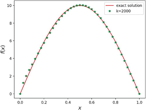
Example 4.1

In the first numerical experiment, we take

(A)	$a\left(x\right)=x^{0.15}$, $f_{\mathrm{t}\mathrm{r}\mathrm{u}\mathrm{e}}\left(x\right)=10\mathrm{s}\mathrm{i}\mathrm{n}\left(\pi x\right)$.
(B)	$a\left(x\right)=x^{0.50}$, $f_{\mathrm{t}\mathrm{r}\mathrm{u}\mathrm{e}}\left(x\right)=10\mathrm{s}\mathrm{i}\mathrm{n}\left(\pi x\right)$.

Figures 1 and 2 show the reconstruction results with diffusion coefficients $a\left(x\right)=x^{0.15}$ and $a\left(x\right)=x^{0.50}$. It can be easily seen that the source term can be recovered very well after 2000 iterations. The relative error between the reconstructed source and the true source is less than $2.20\mathrm{\%}$.

Figure 1. Example 4.1 (A): numerical results for different iteration times, when $a\left(x\right)=x^{0.15}$

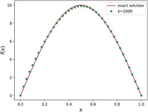
Figure 2. Example 4.1 (B): numerical results for different iteration times, when $a\left(x\right)=x^{0.50}$.

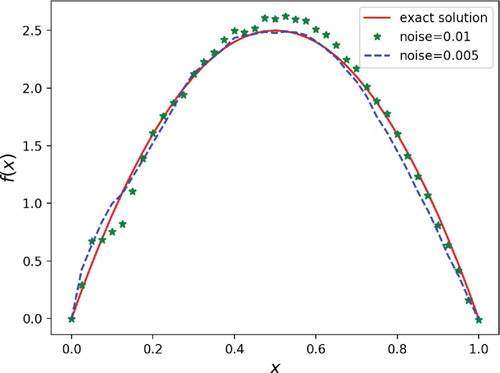
In the following examples, we consider the noisy data generated in the form $u^{\delta }(x,1)=(1+\delta \mathrm{r}\mathrm{a}\mathrm{n}\mathrm{d}(-1,1\left)\right)u\left[f_{\mathrm{t}\mathrm{r}\mathrm{u}\mathrm{e}}\right](x,1),x\in (0,1),$ where rand$(-1,1)$ denotes the uniformly distributed random number in $[-1,1]$ and the noisy levels are $\delta =0.5\mathrm{\%}$ and $\delta =1.0\mathrm{\%}$.

Example 4.2

We consider numerical experiment with noise contaminated observation data.

(A)	$a\left(x\right)=x^{0.15}$, $f_{\mathrm{t}\mathrm{r}\mathrm{u}\mathrm{e}}\left(x\right)=10x(1-x)$.
(B)	$a\left(x\right)=\log (x+1)$, $f_{\mathrm{t}\mathrm{r}\mathrm{u}\mathrm{e}}\left(x\right)=10x(1-x)$.

In Figure 3, the source term is obtained after k = 1073 iteration steps, and the relative error of the reconstructed solution of the inverse source problem is less than $3.99\mathrm{\%}$. In Figure 4, the iteration steps k = 2000 and the relative error is less than $7.02\mathrm{\%}$. Moreover, we can also see that the degeneracy on boundary may produce a relatively large impact on the reconstruction results. It is not difficult to find that the recovered curve for the case $a\left(x\right)=x^{0.15}$ is better than that of the case $a\left(x\right)=\sin x$, particularly near the boundaries. It is not hard to understand because the diffusion coefficient $a\left(x\right)=\sin x$ has much more degeneracy than $a\left(x\right)=x^{0.15}$ at the boundary x = 0.

Figure 3. Example 4.2 (A): numerical results for different noise levels, when $a\left(x\right)=x^{0.15}$.

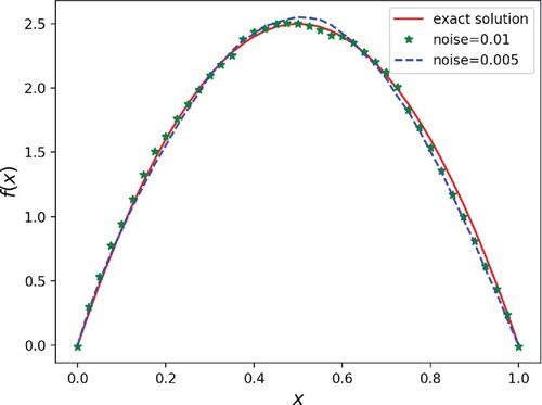
Figure 4. Example 4.2 (B): numerical results for different noise levels, when $a\left(x\right)=\sin x$.

Similarly, the reconstruction of $f_{\mathrm{t}\mathrm{r}\mathrm{u}\mathrm{e}}=1-|2x-1|$ from the noisy data $u^{\delta }(\cdot ,t)$ is also performed.

Example 4.3

We consider numerical experiment with non-differentiable source.

(A)	$a\left(x\right)=x^{0.15}$, $f_{\mathrm{t}\mathrm{r}\mathrm{u}\mathrm{e}}\left(x\right)=1-|2x-1|$.
(B)	$a\left(x\right)=\log (x+1)$, $f_{\mathrm{t}\mathrm{r}\mathrm{u}\mathrm{e}}\left(x\right)=1-|2x-1|$.

The results are shown in Figures 4 and 5, where the noisy levels $\delta =0.5\mathrm{\%}$ and $\delta =1.0\mathrm{\%}$. In Figures 5 and 6, after the iteration steps k = 3000, the source is recovered with the relative error less than $7.12\mathrm{\%}$ and $10.11\mathrm{\%}$ respectively.

Figure 5. Example 4.3 (A): numerical results for different noise levels, when $a\left(x\right)=x^{0.15}$.

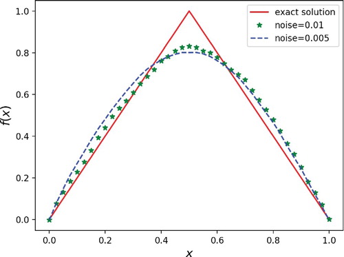
Figure 6. Example 4.3 (B): numerical results for different noise levels, when $a\left(x\right)=\sin x$.

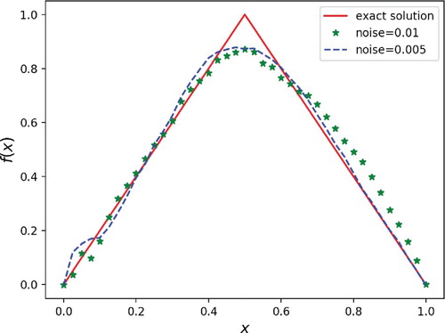
Remark 4.3

Figures 1–4 and the relative errors indicate the efficiency and accuracy of the proposed Algorithm 4.1 for reconstructing the unknown source term. However, it should be mentioned here that owing to the poor regularity of the target function, the reconstruction results are not as well as those of the smooth case in the previous examples.

5. Concluding remarks

In this paper, we considered the inverse problem in reconstructing the source term for the degenerate parabolic equations from the final observation. We first introduced the Hardy type inequality in the framework of weighted Sobolev spaces. We transferred the degenerate equation into a degenerate elliptic one by using finite Laplace transform. As a direct application of the Hardy inequality, we showed that the source term can be uniquely determined from the final state of the solution by the Liouville theorem. By using the integral identity, we further verified the Lipschitz continuous dependency of the source with respect to the final data of the solution with given topology. We should mention that compared with classical parabolic equations, the main difficulty for degenerate equations lies in the degeneracy of the principle coefficients which may lead to the corresponding solution has no sufficient regularity, even if the initial value and the coefficients are sufficiently smooth functions. There will be a challenge if the degenerate equation has flux. Moreover, in the proofs of our results, we need the assumption that all the coefficients are only x-dependent. It will be more interesting and challenging to consider what happens with the properties of the solutions in the case where the coefficients are both t- and x -dependent. It will be also interesting to consider the stability of the inverse source problem if $\rho >0$ in $[0,T]$ is not valid. For example, $\rho \ge 0$.

In the numerical aspect, we reformulated the inverse source problem as an optimization problem with Tikhonov regularization. After the derivation of the corresponding variational equation, we characterized the minimizer by employing the associated backward degenerate parabolic equation, which results in the iterative method. Then several numerical experiments for the reconstructions were implemented to show the efficiency and accuracy of the proposed Algorithm 4.1. Here we should mention that formula (24(24) ${\int }_0^T\rho \left(t\right)v\left[f^{\ast }\right](x,t)\mathrm{d}t+\lambda T{f}^{\ast }\left(x\right)=0,$(24) ) for finding the minimizer of problem (21(21) $\underset{f\in L^2(0,1)}{min}\mathrm{\Phi }\left(f\right),\mathrm{\Phi }\left(f\right):=\parallel u\left[f\right](\cdot ,T)-u^{\delta }(\cdot ,T){\parallel }_{L^2(0,T)}^2+\lambda \parallel f{\parallel }_{L^2(0,1)}^2,$(21) ) is not suitable for f which is not vanished on the boundary. Indeed, for deriving Algorithm 4.1, the homogeneous boundary condition of the solution v to the backward problem was assumed. It will be interesting to derive the iteration scheme without assuming this homogeneous boundary condition on f. The algorithm for the general case remains open.

Acknowledgments

The second author thanks National Natural Science Foundation of China 11801326.

Disclosure statement

No potential conflict of interest was reported by the author(s).

Additional information

Funding

This work was supported by National Natural Science Foundation of China [Grant Number 11801326].

References

- Buchot JM, Raymond JP. A linearized model for boundary layer equations. Optimal control of complex structures (Oberwolfach, 2000). Basel: BirkhNauser; 2002; p. 3–42. (Internat. Ser. Numer. Math.; 139).
- Cannarsa P, Martinez P, Vancostenoble J. Null controllability of degenerate heat equations. Adv Differ Equ. 2005;10:153–190.
- Cannarsa P, Martinez P, Vancostenoble J. Carleman estimates for a class of degenerate parabolic operators. SIAM J Control Optim. 2008;47:1–19. doi: 10.1137/04062062X
- Cannarsa P, Tort J, Yamamoto M. Determination of source terms in a degenerate parabolic equation. Inverse Probl. 2010;26:105003. (20pp) doi: 10.1088/0266-5611/26/10/105003
- Choulli M, Yamamoto M. Generic well-posedness of a linear inverse parabolic problem with diffusion parameters. J Inverse and Ill-Posed Prob. 1999;7(3):241–254.
- Deng ZC, Qian K, Rao XB, et al. An inverse problem of identifying the source coefficient in a degenerate heat equation. Inverse Probl Sci Eng. 2015;23(3):498–517. doi: 10.1080/17415977.2014.922079
- Deng ZC, Yang L. An inverse problem of identifying the coefficient of first-order in a degenerate parabolic equation. J Comput Appl Math. 2011;235(15):4404–4417. doi: 10.1016/j.cam.2011.04.006
- Egger H, Engl HW. Tikhonov regularization applied to the inverse problem of option pricing: convergence analysis and rates. Inverse Problems. 2005;21:1027–1045. doi: 10.1088/0266-5611/21/3/014
- Fotouhi M, Salimi L. Null controllability of degenerate/singular parabolic equations. J Dyn Control Syst. 2012;18(4):573–602. doi: 10.1007/s10883-012-9160-5
- Hasanov A, Slodička M. An analysis of inverse source problems with final time measured output data for the heat conduction equation: A semigroup approach. Appl Math Lett. 2013;26(2):207–214. doi: 10.1016/j.aml.2012.08.013
- Isakov V. Inverse parabolic problems with the final overdetermination. Commun Pure Appl Math. 1991;44(2):185–209. doi: 10.1002/cpa.3160440203
- Jiang LS, Tao YS. Identifying the volatility of underlying assets from option prices. Inverse Probl. 2001;17:137–155. doi: 10.1088/0266-5611/17/1/311
- Li G, Yamamoto M. Stability analysis for determining a source term in a 1-D advection-dispersion equation. J. Inv. Ill-posed Problems. 200614(2):147–155. doi: 10.1515/156939406777571067
- Martinez P, Raymond JP, Vancostenoble J. Regional null controllability of a linearized Crocco-type equation. SIAM J Control Optim. 2003;42:709–728. doi: 10.1137/S0363012902403547
- Oleinik AO, Samokhin VN. Mathematical models in boundary layer theory. Chapman and Hall/CRC; 1999.
- Rundell W, Colton DL. Determination of an unknown non-homogeneous term in a linear partial differential equation, from overspecified boundary data. Applicable Anal. 1980;10(3):231–242. doi: 10.1080/00036818008839304
- Rudin W. Real and complex analysis. Singapore: Tata McGraw-Hill Education; 1987.
- Tort J. Determination of source terms in a degenerate parabolic equation from a locally distributed observation. C R Acad Sci Paris, Ser I. 2010;348:1287–1291. doi: 10.1016/j.crma.2010.10.031
- Tort J, Vancostenoble J. Determination of the insolation function in the nonlinear sellers climate model. Ann I H Poincare-AN. 2012;29:683–713. doi: 10.1016/j.anihpc.2012.03.003
- Rao XB, Wang YX, Qian K. Numerical simulation for an inverse source problem in a degenerate parabolic equation. Appl Math Modelling. 2015;39:23–24. S0307904X15001687. doi: 10.1016/j.apm.2015.03.016
- Yang L, Deng ZC. An inverse backward problem for degenerate parabolic equations. Numer Meth for Partial Differ Equ. 2017;33:1900–1923. doi: 10.1002/num.22165