Non-convex ℓ_p regularization for sparse reconstruction of electrical impedance tomography

Abstract

This work is to investigate the image reconstruction of electrical impedance tomography from the electrical measurements made on an object's surface. An ${\ell }_p$-norm (0<p<1) sparsity-promoting regularization is considered to deal with the fully non-linear electrical impedance tomography problem, and a novel type of smoothing gradient-type iteration scheme is introduced. To avoid the difficulty in calculating its gradient in the optimization process, a smoothing Huber potential function is utilized to approximate the ${\ell }_p$-norm penalty. We then propose the smoothing algorithm in the general frame and establish that any accumulation point of the generated iteration sequence is a first-order stationary point of the original problem. Furthermore, one iteration scheme based on the homotopy perturbation technology is derived to find the minimizers of the Huberized approximated objective function. Numerical experiments show that non-convex ${\ell }_p$-norm sparsity-promoting regularization improves the spatial resolution and is more robust with respect to noise, in comparison with ${\ell }_1$-norm regularization.

Keywords:

• Electrical impedance tomography
• image reconstruction
• regularization methods
• ${\ell }_p$ sparsity minimization

2010 Mathematics Subject Classifications:

• 65N21
• 65R32
• 65J20

1. Introduction

Electrical impedance tomography (EIT) principle is that by applying a constant current across the interested object, the voltage distribution resulting on the surface electrodes will reflect the internal conductivity distribution. In recent years, based on the fast development in imaging technology, EIT with the advantages of low-cost instrumentation, easy portability and non-ionizing radiation is an emerging technology and has attracted considerable interest in medical imaging, geophysical exploration, environmental cleaning and non-destructive testing of materials, etc.

Due to the limited measurement data, image reconstruction in EIT is a highly non-linear ill-posed problem. The ill-posedness makes the conductivity reconstruction extremely sensitive to small perturbation from modelling errors and measurement noise, which causes reconstructed images to still suffer from inherent low spatial resolution and instability. Therefore, various imaging algorithms based on the penalty term regularization have been developed to achieve desired and stable reconstructions, and have delivered very encouraging reconstructions, for example, standard Tikhonov regularization [1], total variation (TV) regularization [2,3], ${\ell }_1$-norm regularization [4–8], and hybrid regularization of several different methods [9–11], etc. The most widespread method is Tikhonov regularization, in which the objective function consists of a quadratic fitting fidelity term and an ${\ell }_2$-norm penalty term, with the aim of matching measurement data and suppressing noises, respectively. However, it often tends to smooth out edges for the reconstructed images in EIT. Another much attention-grabbing method is the ${\ell }_1$-norm regularization, regarded as the convex relaxation of NP-hard $l_0$-norm regularization. It is often used to enforce sparsity and can preserve the details and reduce the noise effect in the reconstruction results effectively. ${\ell }_1$-norm regularization with split-Bregman method is adopted to conduct the EIT imaging problem in [5,11]. It shows that ${\ell }_1$-norm regularization generates more precise reconstructed images compared with classical Tikhonov regularization and TV regularization.

There is already quite a lot of evidence that non-smooth and non-convex regularization terms can provide better reconstruction results than smooth convex or non-smooth convex regularization functions. Recently, many researchers have shown that using the non-smooth and non-convex lower-order ${\ell }_p$-norm (0<p<1) to relax the $l_0$-norm is a better choice than using ${\ell }_1$-norm, and has attracted much attention and has been evidenced in extensive computational studies, see [12–16] and reference therein. However, it is difficult in general to design efficient algorithms for solving ${\ell }_p$ regularized problem. It was presented in [17] that finding the global minimizer is strongly NP-hard; while calculating a local minimum could be done in polynomial time. Some effective and efficient algorithms have been presented to find a local minimizer. In [18,19], based on different ϵ-approximations of ${\ell }_p$-norm, iteratively reweighted algorithms are developed to tackle this approximation problem. In [20,21], the smoothing approaches by adopting smoothing functions are also used to solve non-convex ${\ell }_p$ regularized minimization problem. The critical technique for this type of algorithms is to transform the non-convex and non-smooth sparsity terms into smooth approximate functions by adding relaxation parameters.

The $\ell p$-norm (0<p<1) regularized minimization can produce desirable sparse approximations. This paper is inspired to use $\ell p$-norm (0<p<1) as the penalty term for the EIT image reconstruction, aiming at enforcing better sparsity. In order to make the proposed optimal problem numerically tractable, we first consider the smoothing approximation of the original minimization problem using a smoothing Huber function of the absolute value function. We then present a general frame of the smoothing algorithm and show its convergence. Furthermore, we derive a method based on the homotopy perturbation technology for minimizing this Huberized approximation objective function. The numerical results indicate that ${\ell }_p$-norm ($p\in (0,1)$) regularization promotes the localization of targets and is more robust with respect to noise compared with ${\ell }_1$-norm regularization. In a word, this paper applies non-convex ${\ell }_p$-norm ($p\in (0,1)$) sparsity-promoting regularization combined with a novel gradient-type iteration scheme to investigate the effects of sparsity regularization on the non-linear EIT image reconstruction.

The rest of this paper is built up as follows. Section 2 provides a brief review on the basic mathematical formulation for the EIT problem. In Section 3, we first introduce the smoothing problem to approximate the original ${\ell }_p$ regularized problem by using Huber potential function, and then propose the smoothing algorithm in the general frame and show that any accumulation point of the generated iteration sequence is a stationary point of the original problem. Moreover, one modified Landweber iteration method is formulated for handling the optimization of the smoothing approximation problem. Section 4 reports some numerical simulations to test the performance of our proposed method on experimental data collected on a 2D phantom. Finally, a short conclusion is drawn in Section 5.

2. Forward and inverse models

We shall in this section make a brief review on the basic mathematical formulation for the EIT problem. The image reconstruction in EIT is actually composed of the forward and inverse problems. We first introduce the following notation. Let us consider an open-bounded and simply connected domain $\mathrm{\Omega }\subset {\mathbb{R}}^d(d=2,3)$ with a smooth boundary Γ, and $\{E_{\ell }{\}}_{\ell =1}^L\subset \mathrm{\Gamma }$ be L electrodes which are assumed to be perfect conductors. We assume furthermore that the electrodes $E_{\ell }$ are connected and separated from each other, i.e. ${\overline{E}}_k\bigcap {\overline{E}}_j=o$ for $k\ne j$. The union of the electrode patches is denoted by ${\mathrm{\Gamma }}_e={\cup }_{l=1}^L{E}_{\ell }\subset \mathrm{\Gamma }$. Let $\sigma \in L^{\mathrm{\infty }}\left(\mathrm{\Omega }\right)$ denote the conductivity distribution. The class of admissible conductivities is given by $\mathcal{A}=\{\sigma \in L^{\mathrm{\infty }}(\mathrm{\Omega }):\eta \le \sigma \le {\eta }^{-1}\mathrm{a}.\mathrm{e}.\mathrm{i}\mathrm{n}\mathrm{\Omega },\sigma {|}_{\mathrm{\Gamma }}={\sigma }_0{|}_{\mathrm{\Gamma }}\},$ for some fixed constant $\eta \in (0,1)$, and the condition $\sigma {|}_{\mathrm{\Gamma }}={\sigma }_0{|}_{\mathrm{\Gamma }}$ reflects the fact that inclusions are located inside the object.

2.1. Forward problem and finite element approximation

We consider a typical acquisition experiment for EIT. Assume that L electrodes have been fixed around the surface of the object. Current is injected through some subset of these electrodes to excite the object under investigation, and the induced voltages are measured at all L electrodes. This procedure is repeated many times with different electrodes until a sufficient amount of data has been obtained. Mathematical models for the measurement are described in [22]. The complete electrode model (CEM), as nowadays the standard model for medical applications, includes the effect of the contract impedance, and is accordingly the most accurate physically realizable model for reproducing EIT experimental data, which is defined by Laplace's equation (1) $\mathrm{\nabla }\cdot \left(\sigma \mathrm{\nabla }u\right)=0,\text{in}\mathrm{\Omega }$(1) and the following boundary conditions (2) $\begin{array}{ll}& u+z_{\ell }\sigma \frac{\mathrm{\partial }u}{\mathrm{\partial }n}=U_{\ell },\text{on}{E}_{\ell },\ell =1,2,\dots ,L\\ & {\int }_{E_{\ell }}\sigma \frac{\mathrm{\partial }u}{\mathrm{\partial }n}\mathrm{d}S=I_{\ell },\text{for}\ell =1,2,\dots ,L\\ & \sigma \frac{\mathrm{\partial }u}{\mathrm{\partial }n}=0,\text{on}\mathrm{\Gamma }\setminus {\mathrm{\Gamma }}_e\end{array}$(2) In these equations, u is the electrical potential inside the object domain Ω, $\{z_{\ell }{\}}_{\ell =1}^L$ are the known contact impedance, and n is the unit outward normal to Γ and $\frac{\mathrm{\partial }u}{\mathrm{\partial }n}=\mathrm{\nabla }u\cdot n$, and $U_{\ell }$ and $I_{\ell }$ are the constant potential on electrode ℓth and the current sent to the ℓth electrode, respectively.

Additionally, in order to ensure the solvability and the uniqueness, CEM consists of the elliptic boundary value problem (1(1) $\mathrm{\nabla }\cdot \left(\sigma \mathrm{\nabla }u\right)=0,\text{in}\mathrm{\Omega }$(1) )–(2(2) $\begin{array}{ll}& u+z_{\ell }\sigma \frac{\mathrm{\partial }u}{\mathrm{\partial }n}=U_{\ell },\text{on}{E}_{\ell },\ell =1,2,\dots ,L\\ & {\int }_{E_{\ell }}\sigma \frac{\mathrm{\partial }u}{\mathrm{\partial }n}\mathrm{d}S=I_{\ell },\text{for}\ell =1,2,\dots ,L\\ & \sigma \frac{\mathrm{\partial }u}{\mathrm{\partial }n}=0,\text{on}\mathrm{\Gamma }\setminus {\mathrm{\Gamma }}_e\end{array}$(2) ) together with the following two other conditions for conservation of charge and an arbitrary choice of a ground: (3) $\sum _{\ell =1}^L{I}_{\ell }=0,\sum _{\ell =1}^L{U}_{\ell }=0.$(3) We denote the electrical voltage vector $U=(U_1,U_2,\dots ,U_L{)}^T\in {\mathbb{R}}^L$ and the current vector $I=(I_1,I_2,\dots ,I_L{)}^T\in {\mathbb{R}}^L$.

The EIT forward problem is to calculate potentials u in Ω and U on the electrodes from known conductivity σ, injected currents I, and contact impedances $\{z_{\ell }{\}}_{\ell =1}^L$. In practice, the system (1(1) $\mathrm{\nabla }\cdot \left(\sigma \mathrm{\nabla }u\right)=0,\text{in}\mathrm{\Omega }$(1) )–(3(3) $\sum _{\ell =1}^L{I}_{\ell }=0,\sum _{\ell =1}^L{U}_{\ell }=0.$(3) ) can not be solved analytically for any arbitrary distribution, and therefore numerical approximations must be used to find an approximate solution. The finite element method (FEM) was employed to discretization in simulation, and we refer to [23] for more details on the forward solution and FEM approximation of the CEM.

$H^1\left(\mathrm{\Omega }\right)$ denotes the $L^2\left(\mathrm{\Omega }\right)$-based Sobolev space with smoothness index 1. The weak formulation of the forward problem can be stated as follows: given a current vector $I\in {\mathbb{R}}^L$, a conductivity distribution σ and positive contact impedance $z_l$, to find the solution $(u,U)\in H:=H^1\left(\mathrm{\Omega }\right)\oplus {\mathbb{R}}^L$ such that (4) $b\left(\right(u,U),(v,V\left)\right)=\sum _{l=1}^L{I}_l{V}_l,\mathrm{\forall }(v,V)\in H,$(4) where the strictly elliptic bilinear form b is defined by $b\left(\right(u,U),(v,V\left)\right)={\int }_{\mathrm{\Omega }}\sigma \mathrm{\nabla }u\cdot \mathrm{\nabla }v\mathrm{d}x+\sum _{l=1}^L\frac{1}{z_l}{\int }_{e_l}(u-U_l)(v-V_l)\mathrm{d}S.$ Indeed, the existence and uniqueness of a solution $(u,U)\in H$ has been shown using the Lax–Milgram Lemma in [22].

Then we consider the piecewise linear function $\left\{{\phi }_i\right\}$ as the finite element basis function, and the solution domain Ω will be divided into small triangles elements. We approximate the potential distribution u within Ω as (5) $u^h=\sum _{i=1}^N{\alpha }_i{\phi }_i$(5) and potentials U on the electrodes as (6) $U^h=\sum _{l=1}^{L-1}{\text{β}}_j{n}_j,$(6) where N is the number of nodes in finite element mesh, $n_1=[1,-1,0,\dots ,0{]}^T,n_2=[1,0,-1,0,\dots ,0{]}^T\in {\mathbb{R}}^L$, etc, and ${\alpha }_i$ and ${\text{β}}_j$ are the coefficients to be determined. For notational reasons we identify $u^h$ and $U^h$ with their coordinates and write $u^h=({\alpha }_1,\dots ,{\alpha }_N)$, $U^h=({\text{β}}_1,\dots ,{\text{β}}_{L-1})$. By substituting these two approximations into variational Equation (4(4) $b\left(\right(u,U),(v,V\left)\right)=\sum _{l=1}^L{I}_l{V}_l,\mathrm{\forall }(v,V)\in H,$(4) ) and by choosing $v={\phi }_i$ and $V=n_j$, we obtain a discrete linear system (7) $A\left(\sigma \right)b=f,$(7) where the data vector $f=(\mathbf{0}$, $\hat{I}{)}^T$ with $\mathbf{0}$ $\in {\mathbb{R}}^N$ and $\hat{I}=(I_1-I_2,I_1-I_3,\dots ,I_1-I_L)$, and the determined coefficient vector $b=(u^h,U^h{)}^T$, and the stiffness matrix $\begin{array}{r}A\left(\sigma \right)=\left(\begin{array}{cc}B& C\\ C^T& D\end{array}\right),\end{array}$ with $\begin{array}{rl}{B}_{ij}& ={\int }_{\mathrm{\Omega }}\sigma \mathrm{\nabla }{\phi }_i\cdot \mathrm{\nabla }{\phi }_j\mathrm{d}x+\sum _{\ell =1}^L\frac{1}{z_{\ell }}{\int }_{E_{\ell }}{\phi }_i{\phi }_j\mathrm{d}S,i,j=1,2,\dots ,N,\\ C_{i\ell }& =-\frac{1}{z_{\ell }}{\int }_{E_{\ell }}{\phi }_i\mathrm{d}S,i=1,2,\dots ,N,\ell =1,2,\dots ,L-1,\\ D_{\ell \ell }& =\frac{1}{z_{\ell }}{\int }_{E_{\ell }}\mathrm{d}S,\ell =1,2,\dots ,L-1.\end{array}$ After solving the determined coefficients $b=A(\sigma {)}^{-1}f$, we can use (6(6) $U^h=\sum _{l=1}^{L-1}{\text{β}}_j{n}_j,$(6) ) to find the approximate potentials $U^h$ on the electrodes.

With the aid of the above FEM discretization, a mathematical description between the applied electrode current data I and the computed electrode voltage data $U\left(\sigma \right)$ is provided by the following non-linear forward operator equation (8) $U\left(\sigma \right)=F(\sigma ;I),$(8) where F is the solution operator (also called the forward operator), which depends linearly on I but non-linearly on σ. For a fixed current vector I, we can view $F(\sigma ;I)$ as a function of σ only, i.e. $F\left(\sigma \right)$.

Notice that it is important to distinguish between the PDE operator $A\left(\sigma \right)$ and the forward operator $F\left(\sigma \right)$. Though both are associated with the model problem, their meaning is not the same. Indeed, $A\left(\sigma \right)$ describes the forward problem, while $F\left(\sigma \right)$ actually represents its solution.

2.2. Inverse problem

Assuming measurement data corrupted with additive Gaussian noise e, the mathematical observation model response can be formulated as the fully non-linear operator equation: $U^{\delta }=F\left(\sigma \right)+e.$ In practice, the conductivity distribution σ is not known. What we know is merely all pairs of injected current data and resulting voltage data on the electrodes. Then the EIT inverse problem is to reconstruct the unknown conductivity σ from unavoidably noisy boundary measurement data $U^{\delta }$, also called image reconstruction. EIT image reconstruction can be formulated as minimizing the discrepancy functional between the measurement data and the model predictions in the form: (9) $\underset{\sigma }{min}\mathcal{J}\left(\sigma \right):=\frac{1}{2}\parallel F\left(\sigma \right)-U^{\delta }{\parallel }_2^2,$(9) known as data fidelity.

However, in practice we are limited to a finite number of electrodes and a finite number of current patterns. Due to the limited but noisy measurement data, EIT image reconstruction (9(9) $\underset{\sigma }{min}\mathcal{J}\left(\sigma \right):=\frac{1}{2}\parallel F\left(\sigma \right)-U^{\delta }{\parallel }_2^2,$(9) ) is ill-posed in the sense that small errors in the data can lead to very large deviations in the reconstructions. Hence, some appropriate sort of regularization strategy is beneficial, and it is incorporated into the imaging process, either implicitly or explicitly, in order to obtain physically meaningful images.

3. Inversion approach with ${\ell }_p$ regularization

To combat the ill-posedness, the solution is often constrained by a priori assumption about the conductivity field, e.g. smoothness or sparsity. Application of non-smooth reconstruction techniques is important for EIT imaging process, as it involves discontinuous or small profiles. It has been shown that employing a sparse solver may result in images that show fewer artefacts. This work considers the non-smooth and non-convex ${\ell }_p$ sparsity regularization, which minimizes the following functional (10) $\underset{\sigma }{min}\mathrm{\Phi }\left(\sigma \right):=\mathcal{J}\left(\sigma \right)+\alpha \parallel \sigma {\parallel }_p^p,$(10) where $\parallel \sigma {\parallel }_p:=(\sum _{i=1}^n|{\sigma }_i{|}^p{)}^{\frac{1}{p}}$ with $p\in (0,1)$ is the ${\ell }_p$ quasi-norm, and then takes the minimizer as an approximation to the true conductivity ${\sigma }^{†}$. The scalar $\alpha >0$ is known as a regularization parameter, and controls the tradeoff between the data fidelity term and regularity term.

The choice p = 2 raising the classical smoothness penalty yields the prominent Tikhonov regularization (i.e. ${\ell }_2$ regularization), which provides stability but force solutions to be smooth in some sense thus eliminating the possibility of non-smooth solutions, while the choice $1\le p<2$ also enforces the sparsity and p = 1 results in ${\ell }_1$ sparsity regularization.

Nevertheless, since the ${\ell }_p$ quasi-norm is non-convex and non-smooth, the ${\ell }_p$ regularized minimization problem (10(10) $\underset{\sigma }{min}\mathrm{\Phi }\left(\sigma \right):=\mathcal{J}\left(\sigma \right)+\alpha \parallel \sigma {\parallel }_p^p,$(10) ) is hard to solve; in fact, it is strongly NP-hard [24]. Finding a global minimizer of problem (10(10) $\underset{\sigma }{min}\mathrm{\Phi }\left(\sigma \right):=\mathcal{J}\left(\sigma \right)+\alpha \parallel \sigma {\parallel }_p^p,$(10) ) is much more computational challenges. Non-smoothness for problem (10(10) $\underset{\sigma }{min}\mathrm{\Phi }\left(\sigma \right):=\mathcal{J}\left(\sigma \right)+\alpha \parallel \sigma {\parallel }_p^p,$(10) ) refers to nondifferentiability. Hence it has a difficulty in calculating the gradient in the optimization by use of the gradient-based method. In order to make it numerically tractable, we here consider a smoothing approximation version of this problem. We first establish the smooth approximation of $\parallel \sigma {\parallel }_p^p:=\sum _{i=1}^n|{\sigma }_i{|}^p$ based on a smooth approximate function of the absolute value function.

3.1. Smoothing approximation

Throughout this paper, ${\mathbb{R}}_{+}$ denotes the set of all non-negative (or positive) numbers, and $\parallel \cdot \parallel$ denotes the ${\ell }_2$-norm. For any $\sigma \in {\mathbb{R}}^n$, $|\sigma {|}^p$ denotes an n-dimensional vector whose ith component is $|{\sigma }_i{|}^p$, that is, $|\sigma {|}^p=(|{\sigma }_1{|}^p,\dots ,|{\sigma }_n{|}^p{)}^T$.

Let $g\left(t\right):=|t|=max\{t,-t\}$ for any $t\in \mathbb{R}$, and $g_{\mu }\left(t\right)=\left\{\begin{array}{ll}t,& t\ge \frac{\mu }{2},\\ \frac{t^2}{\mu }+\frac{\mu }{4},& -\frac{\mu }{2}<t<\frac{\mu }{2},\mathrm{\forall }\mu >0,\\ -t,& t\le -\frac{\mu }{2},\end{array}\right.$ and then we have $g_{\mu }\left(t\right)-g\left(t\right)=\left\{\begin{array}{ll}0,& |t|\ge \frac{\mu }{2},\\ \frac{(2t+\mu {)}^2}{4\mu },& -\frac{\mu }{2}<t\le 0,\\ \frac{(2t-\mu {)}^2}{4\mu },& 0\le t<\frac{\mu }{2},\end{array}\right.$ which implies $g\left(t\right)\le g_{\mu }\left(t\right)\le g\left(t\right)+\frac{\mu }{4},\mathrm{\forall }t\in \mathbb{R}$ and hence, $\underset{\mu \to 0^{+}}{lim}{g}_{\mu }\left(t\right)=g\left(t\right).$ Function $g_{\mu }\left(t\right)$ 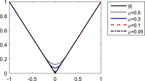is also known as Huber potential function [25,26], which is very often used in robust statistics. Figure 1 shows the graphics of the functions $g\left(t\right)$ and $g_{\mu }\left(t\right)$. It is obviously that the approximation effect is better if smaller the parameter μ. The following simple properties show that the function $g_{\mu }\left(t\right)$ is a nice smoothing approximation of the absolute value function $g\left(t\right)$.

Figure 1. The graphics of $g\left(t\right)$ and $g_{\mu }\left(t\right)$.

Proposition 3.1

For any $(\mu ,t)\in {\mathbb{R}}_{+}\times \mathbb{R},$ we have that

1. $0\le g_{\mu }\left(t\right)-g\left(t\right)\le \frac{\mu }{4},$ and $\underset{\mu \to 0^{+}}{lim}{g}_{\mu }\left(t\right)=g\left(t\right)$.

2. $g_{\mu }\left(t\right)$ is continuously differentiable with (11) $g_{\mu }^{\prime }\left(t\right)=\left\{\begin{array}{ll}1,& t\ge \frac{\mu }{2},\\ \frac{2t}{\mu },& -\frac{\mu }{2}<t<\frac{\mu }{2},\\ -1,& t\le -\frac{\mu }{2}.\end{array}\right.$(11)

3. $|g_{\mu }^{\prime }\left(t\right)|\le 1$ and $\underset{\mu \to 0^{+}}{lim}{g}_{\mu }^{\prime }\left(t\right)=\mathrm{s}\mathrm{i}\mathrm{g}\mathrm{n}\left(\mathrm{t}\right)$.

However, $g_{\mu }\left(t\right)$ is not twice differentiable at $t=\frac{\mu }{2}$. For $t\in (-\frac{\mu }{2},\frac{\mu }{2})$, the second derivative of $g_{\mu }\left(t\right)$ satisfies $g_{\mu }^{″}\left(t\right)=\frac{2}{\mu }>0$, hence $g_{\mu }\left(t\right)$ is strictly convex in $(-\frac{\mu }{2},\frac{\mu }{2})$. For any $\sigma =({\sigma }_1,{\sigma }_2,\dots ,{\sigma }_n{)}^T$, let $G\left(\sigma \right)=\left(g\right({\sigma }_1),g({\sigma }_2),\dots ,g({\sigma }_n){)}^T,$ the cost function $\mathrm{\Phi }\left(\sigma \right)$ can be rewritten as (12) $\mathrm{\Phi }\left(\sigma \right):=\mathcal{J}\left(\sigma \right)+\alpha \parallel G\left(\sigma \right){\parallel }_p^p=\mathcal{J}\left(\sigma \right)+\alpha \sum _{i=1}^n{g}^p\left({\sigma }_i\right),p\in (0,1).$(12) Moreover, let $G_{\mu }\left(\sigma \right)=\left(g_{\mu }\right({\sigma }_1),g_{\mu }({\sigma }_2),\dots ,g_{\mu }({\sigma }_n){)}^T$, and then we have (13) ${\mathrm{\Phi }}_{\mu }\left(\sigma \right):=\mathcal{J}\left(\sigma \right)+\alpha \parallel G_{\mu }\left(\sigma \right){\parallel }_p^p=\mathcal{J}\left(\sigma \right)+\alpha \sum _{i=1}^n{g}_{\mu }^p\left({\sigma }_i\right),p\in (0,1).$(13)

Proposition 3.2

Given $p\in (0,1)$. For any $(\mu ,\sigma )\in {\mathbb{R}}_{+}\times {\mathbb{R}}^n,$ we have $\mathrm{\Phi }\left(\sigma \right)\le {\mathrm{\Phi }}_{\mu }\left(\sigma \right)\le \mathrm{\Phi }\left(\sigma \right)+\alpha n(\mu /4{)}^p.$

Proof.

Using the fact that $g\left({\sigma }_i\right)\le g_{\mu }\left({\sigma }_i\right)\le g\left({\sigma }_i\right)+\frac{\mu }{4}$ for $i=1,2,\dots ,n$, we have that for any $p\in (0,1)$, $g^p\left({\sigma }_i\right)\le g_{\mu }^p\left({\sigma }_i\right)\le \left(g\right({\sigma }_i)+\mu /4{)}^p\le g^p({\sigma }_i)+(\mu /4{)}^p,$ which implies $\sum _{i=1}^n{g}^p\left({\sigma }_i\right)\le \sum _{i=1}^n{g}_{\mu }^p\left({\sigma }_i\right)\le \sum _{i=1}^n\left(g^p\right({\sigma }_i)+(\mu /4{)}^p),$ i.e. (14) $\parallel G\left(\sigma \right){\parallel }_p^p\le \parallel G_{\mu }\left(\sigma \right){\parallel }_p^p\le \parallel G\left(\sigma \right){\parallel }_p^p+\sum _{i=1}^n(\mu /4{)}^p.$(14) Thus, by the definition of $\mathrm{\Phi }\left(\sigma \right)$ and ${\mathrm{\Phi }}_{\mu }\left(\sigma \right)$, it follows that $\mathrm{\Phi }\left(\sigma \right)\le {\mathrm{\Phi }}_{\mu }\left(\sigma \right)\le \mathrm{\Phi }\left(\sigma \right)+\alpha n(\mu /4{)}^p,p\in (0,1),$ which completes the proof.

From Proposition 3.2, it is easy to see that $\underset{\mu \to 0^{+}}{lim}{\mathrm{\Phi }}_{\mu }\left(\sigma \right)=\mathrm{\Phi }\left(\sigma \right).$ It is known that the forward operator $F\left(\sigma \right)$ generated by CEM is uniformly bounded and continuous and is also Fr$\acute{e}$chlet differentiable with respect to conductivity σ. We briefly recall the following property for the forward operator $F\left(\sigma \right)$ (see [27,28]).

Lemma 3.3

Let $I\in {\mathbb{R}}^L$ be a fixed current vector. For any $\sigma ,\sigma +\delta \sigma \in \mathcal{A},$ the forward operator $F\left(\sigma \right)$ is uniformly bounded and continuous and is also Fr$\acute{e}$chlet differentiable with respect to σ. Moreover, the Fr$\acute{e}$chlet derivative $F^{\prime }\left(\sigma \right)$ is bounded and Lipschitz continuous, and the following estimations are satisfied: $\begin{array}{rl}& \parallel F(\sigma +\delta \sigma )-F\left(\sigma \right){\parallel }_H\le C\parallel \delta \sigma {\parallel }_{L^{\mathrm{\infty }}\left(\mathrm{\Omega }\right)},\\ & \parallel F^{\prime }(\sigma +\delta \sigma )-F^{\prime }\left(\sigma \right){\parallel }_{\mathcal{L}\left(L^{\mathrm{\infty }}\right(\mathrm{\Omega }),H)}\le L\parallel \delta \sigma {\parallel }_{L^{\mathrm{\infty }}\left(\mathrm{\Omega }\right)}.\end{array}$

Therefore, for any $\mu >0$, since the function $g_{\mu }$ is continuously differentiable, it follows from (13(13) ${\mathrm{\Phi }}_{\mu }\left(\sigma \right):=\mathcal{J}\left(\sigma \right)+\alpha \parallel G_{\mu }\left(\sigma \right){\parallel }_p^p=\mathcal{J}\left(\sigma \right)+\alpha \sum _{i=1}^n{g}_{\mu }^p\left({\sigma }_i\right),p\in (0,1).$(13) ) that the function ${\mathrm{\Phi }}_{\mu }\left(\sigma \right)$ is continuously differentiable. These demonstrate that the function ${\mathrm{\Phi }}_{\mu }\left(\sigma \right)$ is a nice smoothing approximation of the function $\mathrm{\Phi }\left(\sigma \right)$.

As a consequence, it is very natural that the original variational problem (10(10) $\underset{\sigma }{min}\mathrm{\Phi }\left(\sigma \right):=\mathcal{J}\left(\sigma \right)+\alpha \parallel \sigma {\parallel }_p^p,$(10) ) can be approximated by the following smoothing unconstrained regularized problem (15) $\underset{\sigma }{min}{\mathrm{\Phi }}_{\mu }\left(\sigma \right):=\mathcal{J}\left(\sigma \right)+\alpha \parallel G_{\mu }\left(\sigma \right){\parallel }_p^p,p\in (0,1).$(15) Thus we can design algorithm to solve the minimization problem (15(15) $\underset{\sigma }{min}{\mathrm{\Phi }}_{\mu }\left(\sigma \right):=\mathcal{J}\left(\sigma \right)+\alpha \parallel G_{\mu }\left(\sigma \right){\parallel }_p^p,p\in (0,1).$(15) ) iteratively, and gradually make $\mu \to 0^{+}$ so that a solution of original problem (10(10) $\underset{\sigma }{min}\mathrm{\Phi }\left(\sigma \right):=\mathcal{J}\left(\sigma \right)+\alpha \parallel \sigma {\parallel }_p^p,$(10) ) can be found.

3.2. Convergence of algorithm

We first review the first-order stationary point of (10(10) $\underset{\sigma }{min}\mathrm{\Phi }\left(\sigma \right):=\mathcal{J}\left(\sigma \right)+\alpha \parallel \sigma {\parallel }_p^p,$(10) ) (see, for example, [15,19]).

Definition 3.4

For any $\sigma \in {\mathbb{R}}^n$, let $\mathrm{\Sigma }:=\mathrm{d}\mathrm{i}\mathrm{a}\mathrm{g}\left(\sigma \right)$ denote an $n\times n$ diagonal matrix whose diagonal is formed by the vector σ. $\sigma \in {\mathbb{R}}^n$ is a first-order stationary point of (10(10) $\underset{\sigma }{min}\mathrm{\Phi }\left(\sigma \right):=\mathcal{J}\left(\sigma \right)+\alpha \parallel \sigma {\parallel }_p^p,$(10) ) if (16) $\mathrm{\Sigma }\mathrm{\nabla }\mathcal{J}\left(\sigma \right)+\alpha p|\sigma {|}^p=0,$(16) where $\mathrm{\nabla }\mathcal{J}\left(\sigma \right):=F^{\prime }\left(\sigma {)}^T\right(F\left(\sigma \right)-U^{\delta })$.

Denote the gradient of the regularized penalty term $\parallel G_{\mu }\left(\sigma \right){\parallel }_p^p$ in (15(15) $\underset{\sigma }{min}{\mathrm{\Phi }}_{\mu }\left(\sigma \right):=\mathcal{J}\left(\sigma \right)+\alpha \parallel G_{\mu }\left(\sigma \right){\parallel }_p^p,p\in (0,1).$(15) ) as $G_{\mu ,p}^{\prime }\left(\sigma \right)\triangleq ▽\parallel G_{\mu }\left(\sigma \right){\parallel }_p^p={\left(\frac{\mathrm{\partial }\parallel G_{\mu }\left(\sigma \right){\parallel }_p^p}{\mathrm{\partial }{\sigma }_1},\frac{\mathrm{\partial }\parallel G_{\mu }\left(\sigma \right){\parallel }_p^p}{\mathrm{\partial }{\sigma }_2},\dots ,\frac{\mathrm{\partial }\parallel G_{\mu }\left(\sigma \right){\parallel }_p^p}{\mathrm{\partial }{\sigma }_n}\right)}^T,$ where for any $i=1,2,\dots ,n$, $\frac{\mathrm{\partial }\parallel G_{\mu }\left(\sigma \right){\parallel }_p^p}{\mathrm{\partial }{\sigma }_i}=p{g}_{\mu }^{p-1}\left({\sigma }_i\right)g_{\mu }^{\prime }\left({\sigma }_i\right),$ with $g_{\mu }^{\prime }\left({\sigma }_i\right)$ being calculated by (11(11) $g_{\mu }^{\prime }\left(t\right)=\left\{\begin{array}{ll}1,& t\ge \frac{\mu }{2},\\ \frac{2t}{\mu },& -\frac{\mu }{2}<t<\frac{\mu }{2},\\ -1,& t\le -\frac{\mu }{2}.\end{array}\right.$(11) ). Then the first-order necessary condition of problem (15(15) $\underset{\sigma }{min}{\mathrm{\Phi }}_{\mu }\left(\sigma \right):=\mathcal{J}\left(\sigma \right)+\alpha \parallel G_{\mu }\left(\sigma \right){\parallel }_p^p,p\in (0,1).$(15) ) is given by (17) $\mathrm{\nabla }{\mathrm{\Phi }}_{\mu }\left(\sigma \right)=\mathrm{\nabla }\mathcal{J}\left(\sigma \right)+\alpha G_{\mu ,p}^{\prime }\left(\sigma \right)=0.$(17) This means that ${\sigma }^{\ast }$ is a stationary point of problem (15(15) $\underset{\sigma }{min}{\mathrm{\Phi }}_{\mu }\left(\sigma \right):=\mathcal{J}\left(\sigma \right)+\alpha \parallel G_{\mu }\left(\sigma \right){\parallel }_p^p,p\in (0,1).$(15) ) if it satisfies (17(17) $\mathrm{\nabla }{\mathrm{\Phi }}_{\mu }\left(\sigma \right)=\mathrm{\nabla }\mathcal{J}\left(\sigma \right)+\alpha G_{\mu ,p}^{\prime }\left(\sigma \right)=0.$(17) ).

Based on the cost function ${\mathrm{\Phi }}_{\mu }\left(\sigma \right)$ and its gradient $\mathrm{\nabla }{\mathrm{\Phi }}_{\mu }\left(\sigma \right)$, we in a general framework can present the following smoothing method:

Theorem 3.5

Suppose that the sequence $\left\{{\sigma }_{{\mu }_k}\right\}$ is generated by the above smoothing method. Then

1. Every accumulation point of $\{{\sigma }_{{\mu }_k\}}$ is a stationary point of problem (10(10) $\underset{\sigma }{min}\mathrm{\Phi }\left(\sigma \right):=\mathcal{J}\left(\sigma \right)+\alpha \parallel \sigma {\parallel }_p^p,$(10) ).

2. Let $\left\{{\sigma }_{{\mu }_k}\right\}$ be a sequence of vectors being global minimizers of (15(15) $\underset{\sigma }{min}{\mathrm{\Phi }}_{\mu }\left(\sigma \right):=\mathcal{J}\left(\sigma \right)+\alpha \parallel G_{\mu }\left(\sigma \right){\parallel }_p^p,p\in (0,1).$(15) ) for any given k, then any accumulation point of $\{{\sigma }_{{\mu }_k\}}$ as $k\to \mathrm{\infty }$ is a global minimizer of problem (10(10) $\underset{\sigma }{min}\mathrm{\Phi }\left(\sigma \right):=\mathcal{J}\left(\sigma \right)+\alpha \parallel \sigma {\parallel }_p^p,$(10) ).

Proof.

We first show that the level set $\left\{\sigma |{\mathrm{\Phi }}_{\mu }\right(\sigma )\le {\mathrm{\Phi }}_{\mu }({\sigma }^0\left)\right\}$ for an arbitrary given initial point ${\sigma }^0$ is bounded. If $\left\{\sigma |{\mathrm{\Phi }}_{\mu }\right(\sigma )\le {\mathrm{\Phi }}_{\mu }({\sigma }^0\left)\right\}$ is unbounded, then there exists a sequence $\left\{{\sigma }_{{\mu }_k}\right\}\subset \left\{\sigma |{\mathrm{\Phi }}_{\mu }\right(\sigma )\le {\mathrm{\Phi }}_{\mu }({\sigma }^0\left)\right\}$ such that $\parallel {\sigma }_{{\mu }_k}\parallel \to \mathrm{\infty }$. We have from (14(14) $\parallel G\left(\sigma \right){\parallel }_p^p\le \parallel G_{\mu }\left(\sigma \right){\parallel }_p^p\le \parallel G\left(\sigma \right){\parallel }_p^p+\sum _{i=1}^n(\mu /4{)}^p.$(14) ) that (18) $\begin{array}{rl}{\mathrm{\Phi }}_{\mu }\left(\sigma \right)& =\mathcal{J}\left(\sigma \right)+\alpha \parallel G_{\mu }\left(\sigma \right){\parallel }_p^p\\ & \ge \mathcal{J}\left(\sigma \right)+\alpha (\parallel G\left(\sigma \right){\parallel }_p^p-|\parallel G\left(\sigma \right){\parallel }_p^p-\parallel G_{\mu }\left(\sigma \right){\parallel }_p^p|)\\ & \ge \mathcal{J}\left(\sigma \right)+\alpha \parallel G\left(\sigma \right){\parallel }_p^p-\alpha n(\mu /4{)}^p\\ & =\mathcal{J}\left(\sigma \right)+\alpha \parallel \sigma {\parallel }_p^p-\alpha n(\mu /4{)}^p,\end{array}$(18) and then $\parallel {\sigma }_{{\mu }_k}\parallel \to \mathrm{\infty }$ implies ${\mathrm{\Phi }}_{\mu }\left({\sigma }_{{\mu }_k}\right)\to +\mathrm{\infty }$, which contradicts with the result that ${\mathrm{\Phi }}_{\mu }\left({\sigma }_{{\mu }_k}\right)\le {\mathrm{\Phi }}_{\mu }\left({\sigma }^0\right)$ for all k. Therefore, we can obtain that the sequence $\left\{{\sigma }_{{\mu }_k}\right\}$ is bounded.

Thus, there exists at least a convergent subsequence of $\left\{{\sigma }_{{\mu }_k}\right\}$. Let $\overline{\sigma }$ be an accumulation point of $\left\{{\sigma }_{{\mu }_k}\right\}$, and denote $\underset{k\to \mathrm{\infty }}{lim}{\sigma }_{{\mu }_k}=\overline{\sigma }$ without loss of generality. Let ${\mathrm{\Sigma }}_{{\mu }_k}:=\mathrm{d}\mathrm{i}\mathrm{a}\mathrm{g}\left({\sigma }_{{\mu }_k}\right)$ and $\mathrm{\Sigma }:=\mathrm{d}\mathrm{i}\mathrm{a}\mathrm{g}\left(\overline{\sigma }\right)$.

(i) From the first-order necessary condition (17(17) $\mathrm{\nabla }{\mathrm{\Phi }}_{\mu }\left(\sigma \right)=\mathrm{\nabla }\mathcal{J}\left(\sigma \right)+\alpha G_{\mu ,p}^{\prime }\left(\sigma \right)=0.$(17) ) for problem (15(15) $\underset{\sigma }{min}{\mathrm{\Phi }}_{\mu }\left(\sigma \right):=\mathcal{J}\left(\sigma \right)+\alpha \parallel G_{\mu }\left(\sigma \right){\parallel }_p^p,p\in (0,1).$(15) ), we have $\mathrm{\nabla }{\mathrm{\Phi }}_{{\mu }_k}\left({\sigma }_{{\mu }_k}\right)=\mathrm{\nabla }\mathcal{J}\left({\sigma }_{{\mu }_k}\right)+\alpha G_{{\mu }_k,p}^{\prime }\left({\sigma }_{{\mu }_k}\right)=0.$ Furthermore, (19) ${\mathrm{\Sigma }}_{{\mu }_k}\mathrm{\nabla }{\mathrm{\Phi }}_{\mu }\left({\sigma }_{{\mu }_k}\right)={\mathrm{\Sigma }}_{{\mu }_k}\mathrm{\nabla }\mathcal{J}\left({\sigma }_{{\mu }_k}\right)+\alpha {\mathrm{\Sigma }}_{{\mu }_k}{G}_{{\mu }_k,p}^{\prime }\left({\sigma }_{{\mu }_k}\right)=0.$(19) By the definition of $G_{\mu ,p}^{\prime }$ and the above argument, we have $[{\mathrm{\Sigma }}_{{\mu }_k}{G}_{{\mu }_k,p}^{\prime }\left({\sigma }_{{\mu }_k}\right){]}_i=p\left[{\sigma }_{{\mu }_k}{]}_i{g}_{{\mu }_k}^{p-1}\right(\left[{\sigma }_{{\mu }_k}{]}_i\right)g_{{\mu }_k}^{\prime }\left(\right[{\sigma }_{{\mu }_k}{]}_i),i=1,2,\dots ,n,$ and then we obtain $\underset{k\to \mathrm{\infty }}{lim}[{\mathrm{\Sigma }}_{{\mu }_k}{G}_{{\mu }_k,p}^{\prime }\left({\sigma }_{{\mu }_k}\right){]}_i=\underset{k\to \mathrm{\infty }}{lim}p{\overline{\sigma }}_i{g}_{{\mu }_k}^{p-1}\left({\overline{\sigma }}_i\right)g_{{\mu }_k}^{\prime }\left({\overline{\sigma }}_i\right).$ Since ${\mu }_k\to 0^{+}$ as $k\to \mathrm{\infty }$, it from Proposition 3.1 (i) and (iii) follows that $\underset{k\to \mathrm{\infty }}{lim}[{\mathrm{\Sigma }}_{{\mu }_k}{G}_{{\mu }_k,p}^{\prime }\left({\sigma }_{{\mu }_k}\right){]}_i=p{\overline{\sigma }}_i{g}^{p-1}\left({\overline{\sigma }}_i\right)\mathrm{s}\mathrm{i}\mathrm{g}\mathrm{n}\left({\overline{\sigma }}_i\right)=p|\overline{{\sigma }_i}{|}^p,i=1,2,\dots ,n.$ Therefore, by (19(19) ${\mathrm{\Sigma }}_{{\mu }_k}\mathrm{\nabla }{\mathrm{\Phi }}_{\mu }\left({\sigma }_{{\mu }_k}\right)={\mathrm{\Sigma }}_{{\mu }_k}\mathrm{\nabla }\mathcal{J}\left({\sigma }_{{\mu }_k}\right)+\alpha {\mathrm{\Sigma }}_{{\mu }_k}{G}_{{\mu }_k,p}^{\prime }\left({\sigma }_{{\mu }_k}\right)=0.$(19) ) we have $0=\underset{k\to \mathrm{\infty }}{lim}{\mathrm{\Sigma }}_{{\mu }_k}\mathrm{\nabla }\mathcal{J}\left({\sigma }_{{\mu }_k}\right)+\underset{k\to \mathrm{\infty }}{lim}\alpha {\mathrm{\Sigma }}_{{\mu }_k}{G}_{{\mu }_k,p}^{\prime }\left({\sigma }_{{\mu }_k}\right)=\mathrm{\Sigma }\mathrm{\nabla }\mathcal{J}\left(\overline{\sigma }\right)+\alpha p|\overline{\sigma }{|}^p,$ i.e. $\overline{\sigma }$ satisfies (16(16) $\mathrm{\Sigma }\mathrm{\nabla }\mathcal{J}\left(\sigma \right)+\alpha p|\sigma {|}^p=0,$(16) ), which implies that $\overline{\sigma }$ is a stationary point of problem (10(10) $\underset{\sigma }{min}\mathrm{\Phi }\left(\sigma \right):=\mathcal{J}\left(\sigma \right)+\alpha \parallel \sigma {\parallel }_p^p,$(10) ).

(ii) Let ${\sigma }^{\ast }$ be a global minimizer of (10(10) $\underset{\sigma }{min}\mathrm{\Phi }\left(\sigma \right):=\mathcal{J}\left(\sigma \right)+\alpha \parallel \sigma {\parallel }_p^p,$(10) ). Then from the following three inequalities $\mathrm{\Phi }\left({\sigma }^{\ast }\right)\le \mathrm{\Phi }\left({\sigma }_{{\mu }_k}\right)\le {\mathrm{\Phi }}_{{\mu }_k}\left({\sigma }_{{\mu }_k}\right)\le {\mathrm{\Phi }}_{{\mu }_k}\left({\sigma }^{\ast }\right)\le \mathrm{\Phi }\left({\sigma }^{\ast }\right)+\alpha n({\mu }_k/4{)}^p,$ take $k\in \mathrm{\infty }$, we obtain that $\mathrm{\Phi }\left(\overline{\sigma }\right)=\mathrm{\Phi }\left({\sigma }^{\ast }\right)$. Thus we deduce that $\overline{\sigma }$ is a global minimizer of (10(10) $\underset{\sigma }{min}\mathrm{\Phi }\left(\sigma \right):=\mathcal{J}\left(\sigma \right)+\alpha \parallel \sigma {\parallel }_p^p,$(10) ).

In [15], Chen et al. established lower bounds for the absolute value of non-zero entries in any local optimal solution of ${\ell }_2$-${\ell }_p(0<p<1)$ minimization model. This establishes a theoretical justification by eliminating those small enough entries in an approximate solution and gives an explanation why the ${\ell }_2$-${\ell }_p(0<p<1)$ minimization model generates more sparse solutions when the norm parameter 0<p<1. Below is the lower bound theory for non-zero entries of the stationary point of the smoothing problem (15(15) $\underset{\sigma }{min}{\mathrm{\Phi }}_{\mu }\left(\sigma \right):=\mathcal{J}\left(\sigma \right)+\alpha \parallel G_{\mu }\left(\sigma \right){\parallel }_p^p,p\in (0,1).$(15) ) under the assumption that the smoothing parameter $\mu >0^{+}$ is sufficiently small. The lower bound clearly shows the relationship between the sparsity of the solution and the choice of the regularization parameter.

Theorem 3.6

For any sufficiently small $\mu >0^{+},$ let ${\sigma }_{\mu }^{\ast }$ be a stationary point of problem (15(15) $\underset{\sigma }{min}{\mathrm{\Phi }}_{\mu }\left(\sigma \right):=\mathcal{J}\left(\sigma \right)+\alpha \parallel G_{\mu }\left(\sigma \right){\parallel }_p^p,p\in (0,1).$(15) ) contained in the level set $\left\{\sigma |{\mathrm{\Phi }}_{\mu }\right(\sigma )\le {\mathrm{\Phi }}_{\mu }({\sigma }^0\left)\right\}$ for an arbitrary given initial ${\sigma }^0$. Denote $L:=(\frac{\alpha p}{\text{β}}{)}^{\frac{1}{1-p}}-\frac{\mu }{4},$ then we have $({\sigma }_{\mu }^{\ast }{)}_i\in [-L,L]\Rightarrow |({\sigma }_{\mu }^{\ast }{)}_i|\le \mu /2,i\in \{1,2,\dots ,n\}.$

Proof.

Since ${\sigma }_{\mu }^{\ast }$ is a stationary point of problem (15(15) $\underset{\sigma }{min}{\mathrm{\Phi }}_{\mu }\left(\sigma \right):=\mathcal{J}\left(\sigma \right)+\alpha \parallel G_{\mu }\left(\sigma \right){\parallel }_p^p,p\in (0,1).$(15) ), the corresponding first-order necessary condition gives $\mathrm{\nabla }{\mathrm{\Phi }}_{\mu }\left({\sigma }_{\mu }^{\ast }\right)=\mathrm{\nabla }\mathcal{J}\left({\sigma }_{\mu }^{\ast }\right)+\alpha G_{\mu ,p}^{\prime }\left({\sigma }_{\mu }^{\ast }\right)=0,$ which implies $\parallel \mathrm{\nabla }\mathcal{J}\left({\sigma }_{\mu }^{\ast }\right)\parallel =\parallel \alpha G_{\mu ,p}^{\prime }\left({\sigma }_{\mu }^{\ast }\right)\parallel .$ Using ${\mathrm{\Phi }}_{\mu }\left({\sigma }_{\mu }^{\ast }\right)\le {\mathrm{\Phi }}_{\mu }\left(0\right)$ and the boundedness of the adjoint operator $F^{\prime }(\sigma {)}^{\ast }$, we have (20) $\begin{array}{rl}\parallel \alpha G_{\mu ,p}^{\prime }\left({\sigma }_{\mu }^{\ast }\right){\parallel }_2^2& =\parallel \mathrm{\nabla }\mathcal{J}\left({\sigma }_{\mu }^{\ast }\right){\parallel }_2^2=\parallel F^{\prime }\left({\sigma }_{\mu }^{\ast }{)}^{\ast }\right(F\left({\sigma }_{\mu }^{\ast }\right)-U^{\delta }){\parallel }_2^2\\ & \le \parallel F^{\prime }({\sigma }_{\mu }^{\ast }{)}^{\ast }{\parallel }_2^2(\parallel F({\sigma }_{\mu }^{\ast })-U^{\delta }{\parallel }_2^2+2\alpha \parallel G_{\mu }({\sigma }_{\mu }^{\ast }){\parallel }_p^p)\\ & \le B^2\parallel F\left(0\right)-U^{\delta }{\parallel }_2^2={\text{β}}^2,\end{array}$(20) with a positive constant B, here we can choose $\text{β}=B\parallel F\left(0\right)-U^{\delta }{\parallel }_2$.

Suppose $[{\sigma }_{\mu }^{\ast }{]}_i\in (-L,L)$ but $|[{\sigma }_{\mu }^{\ast }{]}_i|>\mu /2$, then we have that (21) $\begin{array}{rl}\parallel \alpha G_{\mu ,p}^{\prime }\left({\sigma }_{\mu }^{\ast }\right)\parallel & \ge \alpha |\left[G_{\mu ,p}^{\prime }\right(\left[{\sigma }_{\mu }^{\ast }{]}_i\right)|=\alpha p{g}_{\mu }^{p-1}\left(\right[{\sigma }_{\mu }^{\ast }\left){]}_i\right)|g_{\mu }^{\prime }\left(\right[{\sigma }_{\mu }^{\ast }{]}_i)|\\ & \ge \alpha p{\left[g\left(\right[{\sigma }_{\mu }^{\ast }{]}_i)+\mu /4\right]}^{p-1}|g_{\mu }^{\prime }\left(\right[{\sigma }_{\mu }^{\ast }{]}_i)|\\ & \ge \alpha p{\left[|[{\sigma }_{\mu }^{\ast }{]}_i|+\mu /4\right]}^{p-1}.\end{array}$(21) From (20(20) $\begin{array}{rl}\parallel \alpha G_{\mu ,p}^{\prime }\left({\sigma }_{\mu }^{\ast }\right){\parallel }_2^2& =\parallel \mathrm{\nabla }\mathcal{J}\left({\sigma }_{\mu }^{\ast }\right){\parallel }_2^2=\parallel F^{\prime }\left({\sigma }_{\mu }^{\ast }{)}^{\ast }\right(F\left({\sigma }_{\mu }^{\ast }\right)-U^{\delta }){\parallel }_2^2\\ & \le \parallel F^{\prime }({\sigma }_{\mu }^{\ast }{)}^{\ast }{\parallel }_2^2(\parallel F({\sigma }_{\mu }^{\ast })-U^{\delta }{\parallel }_2^2+2\alpha \parallel G_{\mu }({\sigma }_{\mu }^{\ast }){\parallel }_p^p)\\ & \le B^2\parallel F\left(0\right)-U^{\delta }{\parallel }_2^2={\text{β}}^2,\end{array}$(20) ) and (21(21) $\begin{array}{rl}\parallel \alpha G_{\mu ,p}^{\prime }\left({\sigma }_{\mu }^{\ast }\right)\parallel & \ge \alpha |\left[G_{\mu ,p}^{\prime }\right(\left[{\sigma }_{\mu }^{\ast }{]}_i\right)|=\alpha p{g}_{\mu }^{p-1}\left(\right[{\sigma }_{\mu }^{\ast }\left){]}_i\right)|g_{\mu }^{\prime }\left(\right[{\sigma }_{\mu }^{\ast }{]}_i)|\\ & \ge \alpha p{\left[g\left(\right[{\sigma }_{\mu }^{\ast }{]}_i)+\mu /4\right]}^{p-1}|g_{\mu }^{\prime }\left(\right[{\sigma }_{\mu }^{\ast }{]}_i)|\\ & \ge \alpha p{\left[|[{\sigma }_{\mu }^{\ast }{]}_i|+\mu /4\right]}^{p-1}.\end{array}$(21) ), we can get $|[{\sigma }_{\mu }^{\ast }{]}_i|\ge {\left(\frac{\alpha p}{\text{β}}\right)}^{\frac{1}{1-p}}-\frac{\mu }{4}=L.$ This is a contradiction to $[{\sigma }_{\mu }^{\ast }{]}_i\in (-L,L)$. Thus, the desired result holds.

3.3. Homotopy perturbation iteration method

The basic idea of image reconstruction for EIT is to repeatedly solve the forward problem while updating σ according to some criteria. The regularized minimization problem (10(10) $\underset{\sigma }{min}\mathrm{\Phi }\left(\sigma \right):=\mathcal{J}\left(\sigma \right)+\alpha \parallel \sigma {\parallel }_p^p,$(10) ) is complicated by high-degree non-linearity of the forward operator F and non-smoothness of the ${\ell }_p$-norm penalty. Now we focus on the smooth minimization problem (15(15) $\underset{\sigma }{min}{\mathrm{\Phi }}_{\mu }\left(\sigma \right):=\mathcal{J}\left(\sigma \right)+\alpha \parallel G_{\mu }\left(\sigma \right){\parallel }_p^p,p\in (0,1).$(15) ). Problem (15(15) $\underset{\sigma }{min}{\mathrm{\Phi }}_{\mu }\left(\sigma \right):=\mathcal{J}\left(\sigma \right)+\alpha \parallel G_{\mu }\left(\sigma \right){\parallel }_p^p,p\in (0,1).$(15) ) is a continuously differentiable, unconstrained optimization problem.

Homotopy perturbation technology as an effective method has been applied to solve various of non-linear equations in different branches of science and engineering [29–31]. The essential idea is to introduce a homotopy parameter and combine the traditional perturbation method with the homotopy technique. Its most notable feature is that usually only a few perturbation terms can be sufficient to acquire a reasonably accurate solution. It has also been extended to homotopy perturbation iteration (HPI) for solving non-linear ill-posed inverse problems [32–34]. The numerical results show that HPI method can save calculation time and promote calculation efficiency greatly with almost the same accuracy, in contrast to the classical Landweber iteration. In this section, we develop one novel type of iteration scheme combining with the homotopy perturbation technique for problem (15(15) $\underset{\sigma }{min}{\mathrm{\Phi }}_{\mu }\left(\sigma \right):=\mathcal{J}\left(\sigma \right)+\alpha \parallel G_{\mu }\left(\sigma \right){\parallel }_p^p,p\in (0,1).$(15) ).

We first consider the standard local linearized iterative approach for the non-linear inversion model, i.e. using a linearized step at each iteration. Using an iterative framework, and let $F\left(\sigma \right)$ be the first two terms in a Taylors series expansion at ${\sigma }^k$, i.e. $F\left(\sigma \right)\approx F\left({\sigma }^k\right)+J_k(\sigma -{\sigma }^k),$ where $J_k:=F^{\prime }\left({\sigma }^k\right)$ is the Jacobian of the forward operator with respect to σ evaluated at ${\sigma }^k$, our proposed smoothing approximation problem (15(15) $\underset{\sigma }{min}{\mathrm{\Phi }}_{\mu }\left(\sigma \right):=\mathcal{J}\left(\sigma \right)+\alpha \parallel G_{\mu }\left(\sigma \right){\parallel }_p^p,p\in (0,1).$(15) ) becomes that (22) $\underset{\sigma }{min}{\tilde{\mathrm{\Phi }}}_{\mu }\left(\sigma \right):=\frac{1}{2}\parallel J_k(\sigma -{\sigma }^k)+F\left({\sigma }^k\right)-U^{\delta }{\parallel }_2^2+\alpha \parallel G_{\mu }\left(\sigma \right){\parallel }_p^p,p\in (0,1).$(22) Moreover, using the notation $r_k:=F\left({\sigma }^k\right)-U^{\delta }$, the minimizer of (22(22) $\underset{\sigma }{min}{\tilde{\mathrm{\Phi }}}_{\mu }\left(\sigma \right):=\frac{1}{2}\parallel J_k(\sigma -{\sigma }^k)+F\left({\sigma }^k\right)-U^{\delta }{\parallel }_2^2+\alpha \parallel G_{\mu }\left(\sigma \right){\parallel }_p^p,p\in (0,1).$(22) ) satisfies the Euler equation: (23) $\mathrm{\nabla }{\tilde{\mathrm{\Phi }}}_{\mu }\left(\sigma \right)=J_k^T\left(J_k\right(\sigma -{\sigma }^k)+r_k)+\alpha G_{\mu ,p}^{\prime }\left(\sigma \right)=0,$(23) here ${(}^T)$ represents the transpose of a matrix. Setting a fixed point homotopy function $H(\sigma ,\lambda ):R\times [0,1]\to R,$ which satisfies (24) $H(\sigma ,\lambda )=\lambda \left[J_k^T\left(J_k\right(\sigma -{\sigma }^k)+r_k)+\alpha G_{\mu ,p}^{\prime }\left(\sigma \right)\right]+(1-\lambda )(\sigma -{\sigma }^k)=0,$(24) where $\lambda \in [0,1]$ is an embedding homotopy parameter. The corresponding solution σ of (24(24) $H(\sigma ,\lambda )=\lambda \left[J_k^T\left(J_k\right(\sigma -{\sigma }^k)+r_k)+\alpha G_{\mu ,p}^{\prime }\left(\sigma \right)\right]+(1-\lambda )(\sigma -{\sigma }^k)=0,$(24) ) depends on the variable λ, thus it can be regarded as a function of parameter λ, i.e. $\sigma \left(\lambda \right)$. Obviously, from (24(24) $H(\sigma ,\lambda )=\lambda \left[J_k^T\left(J_k\right(\sigma -{\sigma }^k)+r_k)+\alpha G_{\mu ,p}^{\prime }\left(\sigma \right)\right]+(1-\lambda )(\sigma -{\sigma }^k)=0,$(24) ), we will have (25) $\begin{array}{rl}& H(\sigma ,0)=\sigma -{\sigma }^k=0,\\ & H(\sigma ,1)=\mathrm{\nabla }{\tilde{\mathrm{\Phi }}}_{\mu }\left(\sigma \right)=J_k^T\left(J_k\right(\sigma -{\sigma }^k)+r_k)+\alpha G_{\mu ,p}^{\prime }\left(\sigma \right)=0.\end{array}$(25) As the parameter λ changed continuously from 0 to 1, the trivial problem $H(\sigma ,0)=0$ is continuously deformed to the original problem $H(\sigma ,1)=0$, i.e. the function $\sigma \left(\lambda \right)$ changed continuously from ${\sigma }^k$ to the approximate solution σ.

We then further expand $G_{\mu ,p}^{\prime }\left(\sigma \right)$ as a Taylor series at ${\sigma }^k$ and ignore the higher-order term, i.e. (26) $G_{\mu ,p}^{\prime }\left(\sigma \right)=G_{\mu ,p}^{\prime }\left({\sigma }^k\right)+G_{\mu ,p}^{″}\left({\sigma }^k\right)(\sigma -{\sigma }^k),$(26) where $G_{\mu ,p}^{″}\left(\sigma \right)$ denotes the Hessian of $\parallel G_{\mu }\left(\sigma \right){\parallel }_p^p$. Since $g_{\mu }^{″}\left(t\right)\to +\mathrm{\infty }$ as $t\to \left(\frac{\mu }{2}{)}^{-}\mathrm{o}\mathrm{r}\right(-\frac{\mu }{2}{)}^{+}$, the Hessian $G_{\mu ,p}^{″}\left(\sigma \right)$ can be approximated as $G_{\mu ,p}^{″}\left(\sigma \right)=diag(\frac{{\mathrm{\partial }}^2\parallel G_{\mu }\left(\sigma \right){\parallel }_p^p}{{\mathrm{\partial }}^2{\sigma }_1},\frac{{\mathrm{\partial }}^2\parallel G_{\mu }\left(\sigma \right){\parallel }_p^p}{{\mathrm{\partial }}^2{\sigma }_2},\dots ,\frac{{\mathrm{\partial }}^2\parallel G_{\mu }\left(\sigma \right){\parallel }_p^p}{{\mathrm{\partial }}^2{\sigma }_n}),$ with $\frac{{\mathrm{\partial }}^2\parallel G_{\mu }\left(\sigma \right){\parallel }_p^p}{{\mathrm{\partial }}^2{\sigma }_i}\approx p(p-1)g_{\mu }^{p-2}\left({\sigma }_i\right)\left(g_{\mu }^{\prime }\right({\sigma }_i){)}^2,\mathrm{f}\mathrm{o}\mathrm{r}\mathrm{a}\mathrm{n}\mathrm{y}i=1,2,\dots ,n.$ Then we obtain (27) $\begin{array}{rl}& \lambda \left[J_k^T\left(J_k(\sigma -{\sigma }^k)+r_k\right)+\alpha \left(G_{\mu ,p}^{\prime }\left({\sigma }^k\right)+G_{\mu ,p}^{″}\left({\sigma }^k\right)(\sigma -{\sigma }^k)\right)\right]\\ & +(1-\lambda )(\sigma -{\sigma }^k)=0.\end{array}$(27) According to the homotopy perturbation technique, we assume that the solution $\sigma \left(\lambda \right)$ of (27(27) $\begin{array}{rl}& \lambda \left[J_k^T\left(J_k(\sigma -{\sigma }^k)+r_k\right)+\alpha \left(G_{\mu ,p}^{\prime }\left({\sigma }^k\right)+G_{\mu ,p}^{″}\left({\sigma }^k\right)(\sigma -{\sigma }^k)\right)\right]\\ & +(1-\lambda )(\sigma -{\sigma }^k)=0.\end{array}$(27) ) can be expressed as the following power series of λ (i.e. the series solution), (28) $\sigma \left(\lambda \right)=\sum _{n=0}^{\mathrm{\infty }}{\sigma }_n^k{\lambda }^n.$(28) Substituting (28(28) $\sigma \left(\lambda \right)=\sum _{n=0}^{\mathrm{\infty }}{\sigma }_n^k{\lambda }^n.$(28) ) into (27(27) $\begin{array}{rl}& \lambda \left[J_k^T\left(J_k(\sigma -{\sigma }^k)+r_k\right)+\alpha \left(G_{\mu ,p}^{\prime }\left({\sigma }^k\right)+G_{\mu ,p}^{″}\left({\sigma }^k\right)(\sigma -{\sigma }^k)\right)\right]\\ & +(1-\lambda )(\sigma -{\sigma }^k)=0.\end{array}$(27) ) and taking ${\sigma }_0^k:={\sigma }^k$, we can obtain (29) $\begin{array}{rl}& \lambda \left[J_k^T\left(J_k\left(\sum _{n=1}^{\mathrm{\infty }}{\sigma }_n^k{\lambda }^n\right)+r_k\right)+\alpha \left(G_{\mu ,p}^{\prime }\left({\sigma }^k\right)+G_{\mu ,p}^{″}\left({\sigma }^k\right)\left(\sum _{n=1}^{\mathrm{\infty }}{\sigma }_n^k{\lambda }^n\right)\right)\right]\\ & +(1-\lambda )\left(\sum _{n=1}^{\mathrm{\infty }}{\sigma }_n^k{\lambda }^n\right)=0.\end{array}$(29) Equating the coefficients of like powers of λ, we can get (30) $\begin{array}{rl}& {\lambda }^1:{\sigma }_1^k=-[J_k^T{r}_k+\alpha G_{\mu ,p}^{\prime }({\sigma }^k\left)\right];\\ & {\lambda }^n:{\sigma }_n^k=[I-J_k^T{J}_k-\alpha G_{\mu ,p}^{″}({\sigma }^k){]}^n{\sigma }_1^k,n=2,3,\dots \end{array}$(30) As $\lambda \to 1$ for the power series solution (28(28) $\sigma \left(\lambda \right)=\sum _{n=0}^{\mathrm{\infty }}{\sigma }_n^k{\lambda }^n.$(28) ), we get the approximate solution σ of (23(23) $\mathrm{\nabla }{\tilde{\mathrm{\Phi }}}_{\mu }\left(\sigma \right)=J_k^T\left(J_k\right(\sigma -{\sigma }^k)+r_k)+\alpha G_{\mu ,p}^{\prime }\left(\sigma \right)=0,$(23) ), i.e. (31) $\begin{array}{rl}\sigma =\underset{\lambda \to 1}{lim}\sigma \left(\lambda \right)& ={\sigma }_0^k+{\sigma }_1^k+{\sigma }_2^k+\cdots \\ & ={\sigma }_0^k+{\sigma }_1^k+[I-J_k^T{J}_k-\alpha G_{\mu ,p}^{″}({\sigma }^k\left)\right]{\sigma }_1^k+\cdots \\ & ={\sigma }_0^k+\underset{N\to \mathrm{\infty }}{lim}\sum _{n=1}^N[I-J_k^T{J}_k-\alpha G_{\mu ,p}^{″}({\sigma }^k){]}^{n-1}{\sigma }_1^k\end{array}$(31) Following the formula (31(31) $\begin{array}{rl}\sigma =\underset{\lambda \to 1}{lim}\sigma \left(\lambda \right)& ={\sigma }_0^k+{\sigma }_1^k+{\sigma }_2^k+\cdots \\ & ={\sigma }_0^k+{\sigma }_1^k+[I-J_k^T{J}_k-\alpha G_{\mu ,p}^{″}({\sigma }^k\left)\right]{\sigma }_1^k+\cdots \\ & ={\sigma }_0^k+\underset{N\to \mathrm{\infty }}{lim}\sum _{n=1}^N[I-J_k^T{J}_k-\alpha G_{\mu ,p}^{″}({\sigma }^k){]}^{n-1}{\sigma }_1^k\end{array}$(31) ), one iteration scheme can be obtained by the first-order approximation truncation (i.e. N = 1): (32) ${\sigma }^{k+1}={\sigma }^k-{\nu }_k[J_k^T{r}_k+\alpha G_{\mu ,p}^{\prime }({\sigma }^k\left)\right],k=0,1,2,\dots$(32) which is the Landweber iteration (LI) method. When using the second-order approximation truncation (i.e. N = 2), it can yield another novel iteration scheme: (33) ${\sigma }^{k+1}={\sigma }^k-{\nu }_k(2I-J_k^T{J}_k-\alpha G_{\mu ,p}^{″}({\sigma }^k\left)\right)[J_k^T{r}_k+\alpha G_{\mu ,p}^{\prime }({\sigma }^k\left)\right],k=0,1,2,\dots$(33) which is called a homotopy perturbation iteration (HPI) method. Here ${\nu }_k>0$ is an appropriately chosen step size. In fact, a constant step size leads usually to a slow convergence of gradient methods. A proper choice of parameter ${\nu }_k$ in each iteration step is crucial for a satisfying convergence speed of the iteration process. Therefore, we here suggest the following choice of the step size [35]: ${\nu }_k=min\{{\nu }_0\parallel r_k{\parallel }_2^2/\parallel J_k^T{r}_k+\alpha G_{\mu ,p}^{\prime }({\sigma }^k){\parallel }_2^2,{\nu }_1\}$ for some positive constant ${\nu }_0$ and ${\nu }_1$.

In order to use the HPI method to produce a useful approximate solution the iteration must be terminated properly. We will employ the discrepancy principle as a stopping rule, which determines the stopping index $k_{\delta }=k_{\delta }(\delta ,U^{\delta })$ by $\parallel F\left({\sigma }^{k_{\delta }}\right)-U^{\delta }\parallel \le \tau \delta \le \parallel F\left({\sigma }^k\right)-U^{\delta }\parallel ,0\le k<k_{\delta },$ for some sufficiently large $\tau >1$, i.e. ${\sigma }^{k_{\delta }}$ is the calculated approximate solution.

3.4. Algorithm realization

It needs to be emphasized that non-convex ${\ell }_p$ regularization has demonstrated its great potential in recovering sparse parameters (i.e. the number of non-zero elements of parameters is very limited). Next we give some discussion on two types for the sparsity representation as follows:

Case I: the spatial sparsity. The unknown physical conductivity ${\sigma }^{†}$ often consists of the background conductivity ${\sigma }_0$ plus a number of interesting features. Let ${\sigma }_0$ be known and $\delta {\sigma }^{†}:=({\sigma }^{†}-{\sigma }_0)$ be the inhomogeneity conductivity (i.e. inclusions/anomalies). The conductivity fields with simple and small anomalies away from the background will have the spatial sparsity (i.e. most zero elements for the inhomogeneity conductivity $\delta {\sigma }^{†}$). Making use of this a sparsity priori information, instead of attempting to find the approximation σ to ${\sigma }^{†}$, we seek an approximation $\delta \sigma$ to $\delta {\sigma }^{†}$. Therefore, ${\ell }_p$ regularized minimization problem becomes (34) $\underset{\delta \sigma }{min}\mathrm{\Phi }\left(\delta \sigma \right):=\frac{1}{2}\parallel F({\sigma }_0+\delta \sigma )-U^{\delta }{\parallel }_2^2+\alpha \parallel G_{\mu }\left(\delta \sigma \right){\parallel }_p^p,p\in (0,1).$(34) Then we apply the derived HPI scheme to recovery the inhomogeneity $\delta \sigma$, respectively, and can obtain the following form: (35) $\mathrm{H}\mathrm{P}\mathrm{I}:\delta {\sigma }^{k+1}=\delta {\sigma }^k-{\nu }_k(2I-J_k^T{J}_k-\alpha G_{\mu ,p}^{″}(\delta {\sigma }^k\left)\right)[J_k^T{r}_k+\alpha G_{\mu ,p}^{\prime }(\delta {\sigma }^k\left)\right],$(35) and set ${\sigma }^{k+1}={\sigma }_0+\delta {\sigma }^{k+1}$ and repeat the iteration until the stopping rule is achieved.

Case II: the transform domain sparsity. When with a smooth conductivity parameter, we need to resort to the sparsity representation in the transform domain. We can combine the ${\ell }_p$ regularized problem with a wavelet method because a wavelet transformation can convert a smooth parameter into a sparse parameter in the transform domain. Then we arrive at the sparsity-promoting ${\ell }_p$ regularized minimization problem: (36) $\underset{\sigma }{min}\mathrm{\Phi }\left(\sigma \right):=\mathcal{J}\left(\sigma \right)+\alpha \parallel G_{\mu }\left({\sigma }_{\omega }\right){\parallel }_p^p,$(36) where ${\sigma }_{\omega }=W\sigma$ stands for the sparse representation of σ under a transformation matrix W. Using the derived HPI scheme, we can obtain the following form: (37) $\mathrm{W}\mathrm{H}\mathrm{P}\mathrm{I}:{\sigma }^{k+1}={\sigma }^k-{\nu }_k(2I-J_k^T{J}_k-\alpha G_{\mu ,p}^{″}({\sigma }^k\left)\right)[J_k^T{r}_k+\alpha W^T{G}_{\mu ,p}^{\prime }({\sigma }_{\omega }^k\left)\right].$(37)

Finally, the complete minimization procedure is summarized as the following Algorithm 4.

4. Numerical results

In this section, we consider some 2D numerical simulations to demonstrate the performance of our proposed smoothing optimization algorithm. Numerical simulations are conducted to investigate the effect of the ${\ell }_p$-norm regularization with p = 2, 1, 0.5, 0.25 on the EIT image reconstruction. The numerical results are compared with standard Tikhonov regularization and ${\ell }_1$-norm regularization, which is identical to the ${\ell }_p$-norm sparsity regularization with p = 2 and p = 1, respectively. All calculations are done by using MATLAB R2015a on a Lenovo-BTCG00LL with an Intel(R) Core(TM) i7-8550U [email protected] GHz and 8.00 GB memory.

The forward model with CEM was based on the EIDORS toolkit for a linear finite element solver written in Matlab developed by Vauhkonen [36]. A 16 equally spaced electrode system is modelled surrounding two-dimensional circle meshes for simulations. We use constant injection current between adjacent electrodes and adjacent voltage measurement between all other electrodes. Two different finite elements meshes are used for the forward and inverse solvers to avoid inverse crimes. The forward solutions are generated with 1049 nodes and 1968 elements, and the inverse computations are implemented with coarse meshes of 279 nodes and 492 elements to reduce the computational burden. Since we do not perform experimentations, we should obtain the boundary voltage data relying on computer simulation. The noisy measurement data are generated in the form of $U^{\delta }=U^{syn}\left({\sigma }^{†}\right)+\delta \cdot n,$ where $U^{syn}\left({\sigma }^{†}\right)$ denotes the exact synthetic measurements, δ is a relative noise level, and n is the random variable following uniform distribution in [0,1].

Selection of parameters is essential to the quality of reconstructed images, because an inappropriate parameter can lead to a meaningless result. The choice of the regularization parameter α depends on the inversion model and the noise level. Generally speaking, the order of magnitude of α should be in accordance with that of the elements of $F^{\prime }\left({\sigma }_0{)}^T{F}^{\prime }\right({\sigma }_0)$. In all numerical results, the regularization parameter α is selected by experience for relative optimal value. We choose ${\mu }_0=1$, $q_{\mu }=0.5$, set $\tau =20$ for the discrepancy criterion, and take the initial guess ${\sigma }^0$ as the background conductivity. We choose the step length ${\nu }_k$ with ${\nu }_0=0.5$ and ${\nu }_1=1000$. Reconstructed image quality is quantitatively evaluated by relative error (RE) with respect to the true phantom, where RE=$\parallel \sigma -{\sigma }^{true}\parallel /\parallel {\sigma }^{true}\parallel$. A smaller image error indicates a better image quality.

In our simulations, a circular domain which contains different inclusions is investigated. Figure 2 shows four numerical phantom models used for testing our proposed method. The phantoms from left to right have various inclusions. The resistivity values are 4 $\mathrm{\Omega }m$ for the background, 1 Ωm for the blue colour parts and 8 Ωm for the red colour parts. Unless stated, all reconstructed images next will be displayed by the unified colorbars from 1 to 8.

Figure 2. Three simulation phantoms. (a) Phantom A. (b) Phantom B. (c) Phantom C. (d) Phantom D.

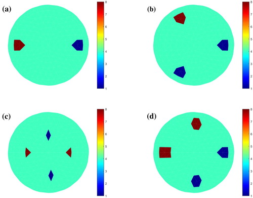
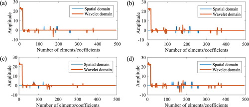
Figure 3. Comparison for sparsity graph of the elements of inhomogeneities and sparsity graph of the haar wavelet coefficients. (a) Phantom A. (b) Phantom B. (c) Phantom C. (d) Phantom D.

In this simulation, let the background conductivity ${\sigma }_0$ be known, and we consider the spacial sparsity for the inhomogeneity conductivity $\delta {\sigma }^{†}$. The reconstructions for case I by LI method and HPI method with p = 0.5 are performed and discussed. We report the performance of reconstructions under noise levels $\delta =0.5\mathrm{\%}$ and $\delta =0.1\mathrm{\%}$ in terms of the number of iteration (Iters), CPU running time (minutes) and relative error (RE). For each noise level, Table 1 shows the reconstructed results. Numerical results show that HPI method reduces the number of iterations and saves the amount of computational time especially for smaller noise level, and produces more accurate results in terms of image error than LI method. This also demonstrates that HPI method has a remarkable acceleration effect. Meanwhile, as can be expected, a little deterioration in the spatial resolution shows with the increase of noise level. In order to visualize the reconstruction accuracy of LI method and HPI method, we next plot the reconstructed images in the third column of Figure 4, which appears the acceptable results.

Figure 4. Reconstructions for various parameter p. (a) Using noisy data with noise level $\delta =0.1\mathrm{\%}$. (b) Using noisy data with noise level $\delta =0.5\mathrm{\%}$. (All displayed by the unified colorbars from 1 to 8.)

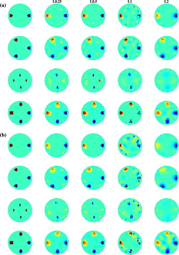
Table 1. Numerical results for case I by LI and HPI method with p = 0.5 under two different noise levels δ.

Phantoms	δ	α	Method	Iters	CPU(m)	RE
Phantom A	$0.5\mathrm{\%}$	1.02e−4	LI	456	1.15	0.0733
			HPI	170	0.47	0.0609
	$0.1\mathrm{\%}$	1.15e−5	LI	2145	5.09	0.0590
			HPI	1438	3.37	0.0561
Phantom B	$0.5\mathrm{\%}$	1.15e−4	LI	174	0.41	0.0946
			HPI	114	0.22	0.0892
	$0.1\mathrm{\%}$	7.25e−6	LI	2389	5.34	0.0769
			HPI	2157	4.98	0.0721
Phantom C	$0.5\mathrm{\%}$	4.35e−5	LI	1392	3.13	0.1164
			HPI	1248	2.93	0.1157
	$0.1\mathrm{\%}$	8.50e−6	LI	9769	21.92	0.0785
			HPI	5296	12.81	0.0692
Phantom D	$0.5\mathrm{\%}$	1.14e−4	LI	486	1.26	0.1094
			HPI	428	0.97	0.0972
	$0.1\mathrm{\%}$	1.40e−5	LI	2493	5.94	0.0862
			HPI	2301	5.42	0.0828

In Figure 3, we display the comparison for sparsity graph of the elements of inhomogeneities and sparsity graph of the haar wavelet coefficients. It can be seen that most elements/coefficients are around zero, that is, there exist many small elements/coefficients. Hence both the inhomogeneity of space domain and the Haar wavelet transformation can effectively provide one sparsity representation. The less bumps show that the sparsity degree is better. Figure 3 obviously shows that there is better sparsity for the spatial domain. Indeed, the effective sparsity representation is key and the sparsity degree impacts the imaging results. Table 2 lists the comparison of reconstructed image errors by HPI method at the noise level $\delta =0.5\mathrm{\%}$ with Case I and Case II, respectively. As we are expected, HPI method with Case I obtains better results because of better sparsity, especially for Phantom A and Phantom D.

Table 2. Comparison of RE for Case I and Case II by HPI under $\delta =0.5\mathrm{\%}$.

Phantoms	Phantom A	Phantom B	Phantom C	Phantom D
Case I	0.0609	0.0892	0.1157	0.0972
Case II	0.0919	0.0994	0.1169	0.1439

Finally, we compare the reconstructed images by ${\ell }_p$ regularization for various parameter p. The studies in [17] have demonstrated that ${\ell }_p(0<p<1)$ regularizer can be represented by the ${\ell }_{1/2}$ regularizer because when $\frac{1}{2}<p<1$, the ${\ell }_{1/2}$ regularizer always yields the best sparse solution and when $0<p<\frac{1}{2}$, the ${\ell }_{1/2}$ regularizer has a sparse property similar to that of the ${\ell }_p$ regularizer. Hence, in Figure 4, depicted with the same colour scale for all images, we show the reconstructions using ${\ell }_p$ sparsity regularization with HPI method for p = 1, 0.5, 0.25 under two various noise levels, and the results are compared with Tikhonov regularization which is identical to the ${\ell }_p$ regularization with p = 2. It is visible that severe artefacts strongly appear with the larger noise in the input data when p = 1. But the non-convex ${\ell }_p$-norm sparsity regularization removes the artefacts, and especially yields better reconstructions with sharper edges and less artefacts when p = 0.5. The noconvex ${\ell }_p$-norm sparsity regularization is effective to enhance the localization and reduce the artefacts. It is clear that a little deterioration in the spatial resolution shows with smaller inclusions for Phantom C since maybe more measurement information is required. Thus it can be seen from Figure 4 that the ${\ell }_p$-norm sparsity regularization reduces the influences of noise and is effective to improve the quality of the reconstructed images.

5. Conclusion

This work investigates the effect of ${\ell }_p$-norm (0<p<1) sparsity-promoting regularization on imaging quality of the fully non-linear EIT inverse problem. Due to the involved non-smoothness, the proposed gradient-based non-linear iteration scheme combines a smoothing function to approximate the ${\ell }_p$-norm penalty. Numerical simulations with synthetic data are carried out to evaluate the feasibility and effectiveness. Results show that non-convex ${\ell }_p$-norm sparsity regularization can improve the spatial resolution and the robustness to noise, and appears to yield reconstructions superior to the ones obtained by $l_1$-norm regularization. In order to obtain more effective sparse representation in the transformation domain, we next will focus on the study of adaptive sparse representation with a merit of representing flexibly when maintaining features of inclusions. Using HR rule to choose the regularization parameter will also be our next work.

Acknowledgements

The author thanks the four anonymous referees for useful comments and suggestions which improve the presentation of the paper.

Disclosure statement

No potential conflict of interest was reported by the authors.

Additional information

Funding

This work was supported by Heilongjiang University Scientific Staring Research Foundation (No. RCCX201719), partly supported by Heilongjiang Provincial Key Laboratory for Complex Systems Theory and Computation (No. 201907), and partly supported by the Fundamental Research Funds for the Universities of Heilongjiang Province-Heilongjiang University Special Fund Project (No. RCYJTD201804).

References

- Vauhkonen M, Vadsz D, Karjalainen PA, et al. Tikhonov regularization and prior information in electrical impedance tomography. IEEE Trans Med Imaging. 1998;17(2):285–293.
- Borsic A, Graham BM, Adler A, et al. Total variation regularization in electrical impedance tomography. Inv Probl. 2007;99:A12.
- Hinze M, Kaltenbacher B, Quyen TNT. Identifying conductivity in electrical impedance tomography with total variation regularization. Numerische Mathematik. 2018;138(3):723–765.
- Jin B, Khan T, Maass P. A reconstruction algorithm for electrical impedance tomography based on sparsity regularization. Int J Numer Methods Eng. 2012;89(3):337–353.
- Wang J, Ma J, Han B, et al. Split Bregman iterative algorithm for sparse reconstruction of electrical impedance tomography. Signal Process. 2012;92(12):2952–2961.
- Gehre M, Kluth T, Sebu C, et al. Sparse 3D reconstructions in electrical impedance tomography using real data. Inv Prob Sci Eng. 2014;22(1):31–44.
- Pham Muoi Q. Reconstructing conductivity coefficients based on sparsity regularization and measured data in electrical impedance tomography. Inv Prob Sci Eng. 2015;23(8):1366–1387.
- Garde H, Knudsen K. Sparsity prior for electrical impedance tomography with partial data. Inv Prob Sci Eng. 2016;24(3):524–541.
- Chung ET, Chan TF, Tai XC. Electrical impedance tomography using level set representation and total variational regularization. J Comput Phys. 2005;205(1):357–372.
- Liu J, Ling L, Li G. A novel combined regularization algorithm of total variation and Tikhonov regularization for open electrical impedance tomography. Phys Meas. 2013;34(7):823.
- Wang J, Han B, Wang W. Elastic-net regularization for nonlinear electrical impedance tomography with a splitting approach. Appl Anal. 2019;98(12):2201–2217.
- Chartrand R. Exact reconstruction of sparse signals via nonconvex minimization. IEEE Signal Process Lett. 2007;14(10):707–710.
- Nikolova M, Ng M, Zhang S, et al. Efficient reconstruction of piecewise constant images using nonsmooth nonconvex minimization. SIAM J Imaging Sci. 2008;1(1):2–25.
- Xu ZB, Zhang H, Wang Y, et al. L1/2 regularization. Sci China Series F (Inf Sci),. 2010;53(6):1159–1169.
- Chen X, Xu F, Ye Y. Lower bound theory of nonzero entries in solutions of l2−lp minimization. SIAM J Sci Comput. 2010;32(5):2832–2852.
- Lai MJ, Wang J. An unconstrained lq minimization with 0<q≤1 for sparse solution of underdetermined linear systems. SIAM J Optim. 2011;21(1):82–101.
- Ge D, Jiang X, Ye Y. A note on the complexity of ℓp minimization. Math Program. 2011;129(2):285–299.
- Chen X, Zhou W. Convergence of the reweighted ℓ1 minimization algorithm for ℓ2−ℓp minimization. Comput Optim Appl. 2014;59(1–2):47–61.
- Lu Z. Iterative reweighted minimization methods for lp regularized unconstrained nonlinear programming. Math Program. 2014;147(1–2):277–307.
- Chen X, Zhou W. Smoothing nonlinear conjugate gradient method for image restoration using nonsmooth nonconvex minimization. SIAM J Imaging Sci. 2010;3(4):765–790.
- Chen X. Smoothing methods for nonsmooth. nonconvex minimization. Math Program. 2012;134(1):71–99.
- Somersalo E, Cheney M, Isaacson D. Existence and uniqueness for electrode models for electric current computed tomography. SIAM J Appl Math. 1992;52(4):1023–1040.
- Woo EJ, Hua P, Webster JG, et al. Finite-element method in electrical impedance tomography. Med Biol Eng Comput. 1994;32(5):530–536.
- Chen X, Ge D, Wang Z, et al. Complexity of unconstrained ℓ2- ℓp minimization. Math Program. 2014;143(1–2):371–383.
- Huber PJ. Robust statistics. New York (NY): John Wiley and Sons; 1981.
- Black MJ, Rangarajan A. On the unification of line processes, outlier rejection, and robust statistics with applications in early vision. Int J Comp Vis. 1996;19(1):57–91.
- Lechleiter A, Rieder A. Newton regularizations for impedance tomography: convergence by local injectivity. Inv Prob. 2008;24(6):065009.
- Jin B, Maass P. An analysis of electrical impedance tomography with, applications to Tikhonov regularization. ESAIM Control Optim Calcul Var. 2012;18(4):1027–1048.
- He JH. Homotopy perturbation technique. Comp Methods Appl Mech Eng. 1999;178(3–4):257–262.
- He JH. Homotopy perturbation method for bifurcation of nonlinear problems. Int J Nonlin Sci Numer Simul. 2005;6(2):207–208.
- Jafari H, Momani S. Solving fractional diffusion and wave equations by modified homotopy perturbation method. Phys Lett A. 2007;370(5–6):388–396.
- Cao L, Han B, Wang W. Homotopy perturbation method for nonlinear ill-posed operator equations. Int J Nonlin Sci Numer Simul. 2009;10(10):1319–1322.
- Wang J, Wang W, Han B. An iteration regularization method with general convex penalty for nonlinear inverse problems in Banach spaces. J Comput Appl Math. 2019;361:472–486.
- Long H, Han B, Tong S. A new Kaczmarz type method and its acceleration for nonlinear ill-posed problems. Inv Probl. 2019;35:055004.
- Jin Q, Wang W. Landweber iteration of Kaczmarz type with general non-smooth convex penalty functionals. Inv Probl. 2013;29(8):085011.
- Vauhkonen M, Lionheart WRB, Heikkinen LM, et al. A matlab package for the EIDORS project to reconstruct two-dimensional EIT images. Physiol Meas. 2001;22(1):107–111.