Inverse analysis of the time-dependent heat flux in stagnation point flow of incompressible fluid impinging on a cylinder with uniform surface suction-blowing using Levenberg–Marquardt method

ABSTRACT

In this paper for the first time, a numerical code based on Levenberg–Marquardt method is presented for solving inverse heat transfer problem of axisymmetric stagnation flow impinging on a cylinder with uniform transpiration and to estimate the time-dependent heat flux using temperature distribution at a point. $\overline{k}$ The effect of noisy data on the final result is studied. The maximum value of the sensitivity coefficient is related to estimation of exponential heat flux and its value is 0.1718 also the minimum value of the sensitivity coefficient is 7.50 × 10⁻⁶ which is related to the triangular heat flux. The results show that the parameter estimation error in calculating the triangular and trapezoidal heat flux is greater than the exponential and sinus–cosines heat flux because the maximum value of RMS error is obtained for these two cases, which are 0.458 and 0.492, respectively the reason for the increase in error in estimating these functions is the existence of points where the first derivative of the function does not exist. This method also exhibits considerable stability for noisy input data. In most cases, surface blowing decreases the prediction accuracy by removing the boundary layers from the surface whereas suction acts vice versa.

KEYWORDS:

• Inverse heat transfer
• Levenberg–Marquardt method
• time-dependent heat flux
• axisymmetric stagnation flow
• uniform transpiration
• noisy data

1. Introduction

Direct heat transfer problem deals with determining the temperature of internal points of a region when the initial and boundary conditions, as well as the thermo physical characteristics, heat generation, heat flux or the wall temperature are known [1]. Unlike direct problems, the inverse heat transfer problems are defined as the estimation of initial and boundary conditions, material characteristics, source and sink terms and the governing equations by considering the distribution of the measured temperature in one or more internal points [2].

In view of the solution stability, inverse problems are much harder to solve compared to direct problems. Mathematically, these types of problems are called ill-posed problems. In recent decades, through the emerging advanced computers, the inverse solution techniques have gained a more general application beyond heat transfer problems. For example, some of the main applications of inverse heat transfers include cooling control of electrical equipment, estimation of cooling jet velocity in machining and quenching hardening process, determination of boundary conditions between mold and the molten metal in casting and rolling processes [3], heat flux determination on a wall surface exposed to fire or inside the surface of a combustion chamber [4] as well as the surfaces where ablation or melting occurs [5]. Other uses of inverse heat transfer include the prediction of the internal wall of reactors, determining thermal conduction coefficient and the external surface conditions in the re-entry of a space vehicle, temperature or heat flux distribution modelling at the tool–work interface of machine cutting [6] and cooling control problems [7]. Different solution methods are applied to inverse heat transfer problems, some of which include exact solutions, inverse transform of Duhamel integral, Laplace transformation, control volume method, Helmholtz equations, finite difference, finite element approximation, digital filter synthesis, Tikhonov regularization, Elifanov iteration method, conjugate gradient and Levenberg–Marquardt methods [8]. Levenberg–Marquardt method is an iterative inverse algorithm based on minimizing the least-square summation of the error values and is employed in this paper.

Jiang et al. [9] obtained the time-dependent boundary heat flux on a solid bar using conjugate gradient method with an adjoint equation and zeroth-order Tikhonov regularization approach to make the inverse solution stable. In their work, finite difference method was used to solve the problem.

Chen et al. [10] derived the temperature and heat flux distribution of the quenching surface using the inverse technique. Finite element techniques were employed to solve the governing equations.

Plotkowski and Krane [11] examined the use of inverse heat conduction models to estimate transient heat flux in electroslag remelting. They studied three inverse heat transfer methods for industrial applications. Hsu et al. [12] applied the inverse problem on wall heat flux estimation to film-wise condensation on vertical surface. Khaniki and Karimian [13] used temperature data to get the heat flux absorbed on a satellite surface. They proposed a simple heat flux sensor to examine the related probable limitations.

Some researches for estimating of heat flux entering the surface of a body using the inverse approach have been presented by Beck et al. [14].

Liu [15] developed a hybrid mechanism to simultaneously identify the thermal conductivity and heat capacity in an inverse heat flux problem. This mechanism was a combination of genetic algorithm and Levenberg–Marquardt algorithms. Mohammadiun et al. [16] estimated the time-dependent heat flux using temperature at a point. Their method included the use of finite difference method to solve the governing equations. Tai et al. [17] applied an inverse conduction heat transfer method to estimate spatial and temporal variation of heat flux on the drilled-hole wall surfaces. Rahimi et al. [18] estimated the time-dependent strength of a heat source using temperature distribution at a point in a three-layer system. Mohammadiun et al. [19] used the sequential function specification method for heat flux prediction on the sublimation boundaries of decomposing materials. Mohammadiun et al. [20] applied sequential function specification method to the ablative surfaces. The inverse method has been used in the mentioned study to estimate of heat flux at the moving interface.

Wu et al. [21] proposed an inverse algorithm based on the conjugate gradient method to solve hyperbolic heat conduction problem and estimate the unknown heat flux on an infinite cylinder.

The estimation of both unknown base temperatures and heat fluxes in the rectangular fin by combining the adjoint conjugate gradient method (ACGM) and lattice Boltzmann method (LBM) has been presented by Bamdad et al. [22]. An inverse method for the estimation of the unknown temperature distribution of the outer surface and the geometry of the inner surface for a furnace with two layer walls has been proposed by Chen et al. [23]. Experimental study on the flow of a liquid film on one of the plates of a vertical channel covered with a porous layer has been presented by Terzi et al. [24].

A comprehensive thermal analysis of an electric machine by combining a numerical model with the determined experimental parameters estimated from an inverse identification method has been presented by Hey et al. [25].

An inverse heat transfer approach based on homotopy analysis method and genetic algorithm has been applied by Panda et al. [26] to estimate the unknown thermal and geometrical configurations of the fin. Thermal performance and inverse optimization of the absorber plate in a flat plate solar collector, along with two different models of heat transfer (Fourier and non-Fourier) and applying convective boundary conditions, have been studied by Panda et al. [27]. Lee et al. [28] applied conjugate gradient method to inverse estimation of unknown time-dependent base heat flux of a functionally graded fin, while knowing temperature history at some measurement locations.

Inverse analysis method based on measured temperatures at the various locations of casting, neural network with back-propagation algorithm and numerical simulation has been performed to define the casting-metal mold IHTC between the casting and metal mold by Zhang et al. [29].

Solution to Navier–Stokes equations generally involves high mathematical complexity. This is due to the non-linearity of these equations such that the superposition theory, used for potential flow, is not applicable. However, for some cases exact solution to Navier–Stokes can be obtained when the nonlinear advection terms are naturally eliminated. Exact solution to stagnation flow problem was initially achieved by Hiemenz [30]. He examined two-dimensional stagnation flow against a flat plate and assumed the stagnation flow on the flat plate to be laminar, incompressible and steady. Following Hiemenz and Homann [31] achieved an exact solution to the three-dimensional Navier–Stokes equations for axisymmetric stagnation flow against a flat plate. Using an appropriate variable change and transforming velocity components into a similarity function, Homann reached an ordinary differential equation for the similarity function with a relevant power series solution. Howarth [32] and Davey [33] reported their researches on the three-dimensional stagnation flow against a flat plate for unaxisymmetric cases. The first exact solution to axisymmetric stagnation flow on an infinite cylinder was reported by Wang [34]. He assumed a stationary cylinder with no rotational or axial movement and no suction and blowing on the cylinder wall. In a series of studies [35–38], Gorla analysed the axisymmetric stagnation flow around a cylinder with laminar flow in steady and transient states. In these works, the effect of uniform axial movement as well as the harmonic axial movement of the cylinder was studied. Cunning et al. [39] carried out research into the effect of cylinder rotation with constant rotational velocity on the stagnation flow over the cylinder. In this research, the effect of uniform suction and blowing on the cylinder wall was also considered. Takhar et al. [40] evaluated the effect of unsteady axisymmetric radial stagnation flow on the cylinder together with the effect of variable-speed axial cylinder movement.

Saleh and Rahimi [41–43] reached exact solutions for axisymmetric stagnation flows on an infinite cylinder and the related heat transfer for cases where the cylinder has time-dependent axial and rotational movement. Further, Shokrgozarabbasi and Rahimi [44–47] proposed exact solution to the three-dimensional stagnation flow and the transient heat transfer of viscous flow impinging on a flat plate. In addition, in a series of studies [48–51], Mohammadiun et al. proposed self-similar solutions of radial stagnation point flow and heat transfer of a viscous, compressible fluid impinging on a cylinder in steady state. They further studied the axisymmetric stagnation flow of a nanofluid on a cylinder for a steady flow when the cylinder wall is exposed to both a constant heat flux and constant temperature [52, 53]. Zahmatkesh et al. [54] evaluated the rate of entropy generation in an axisymmetric stagnation flow of aluminum oxide nanofluid on a stationary cylinder. The effects of uniform suction and blowing as well as the volume fraction of the nanoparticles on the rate of entropy generation are also studied in the mentioned work.

Axisymmetric stagnation flow of a steady micropolar fluid impinging on an infinite circular cylinder has been considered by Hassanien et al. [55]. They applied a new procedure based on Chebyshev approximation to solve the boundary layer equations. In next study, Hassanien et al. [56] analysed heat transfer of a steady micro polar fluid in the vicinity of an axisymmetric stagnation point flow on a circular cylinder.

Nonlinear coupled differential equations governing the stagnation flow at a blunt body have been solved using Chebyshev expansion formulation by Hassanien [57]. This method is accomplished starting with a Chebyshev approximation for the higher order derivatives and generating approximations to the lower order derivatives.

Lin et al. [58] used a diesel spray in the stag nation point flow to experimental investigation of spray burner influences on the flow and flame characteristics of a premixed methane flame.

As can be seen, inverse heat transfer in the vicinity of stagnation region of impinging flow has not been considered yet. All articles on stagnation point flow only deal with the direct problem with known boundary conditions. However, in many real cases, accurate information about unknown wall heat flux is not available in this paper, for the first time a numerical code based on Levenberg–Marquardt method is proposed to solve the inverse time-dependent boundary heat flux for an axisymmetric stagnation flow on a cylinder with uniform suction-blowing. The algorithm uses the temperature distribution at a point and a semi-similar solution. At every time step, the governing equations are converted to a system of coupled ordinary differential equations which, through discretization using implicit finite difference method, are solved by tri-diagonal matrix algorithm (TDMA). Sensitivity to noisy data is evaluated. The results demonstrate considerable stability of the proposed method to noisy data. Due to the complexity of the governing equations in convective heat transfer (Coupled Momentum and Energy equations), we could not find adjoint equation thus we used Levenberg–Marquardt method instead of conjugate gradient method for estimating unknown boundary conditions.

2. Problem formulation

2.1. Direct solution

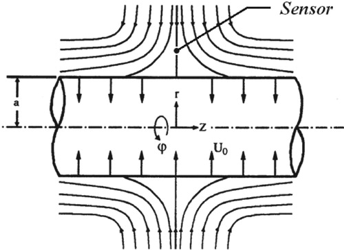
The geometry of this problem is depicted in Figure 1. As shown, the flow is axisymmetric in cylindrical coordinates $(r,z)$ with corresponding velocity components (u, w). Time-dependent heat flux and uniform transpiration are applied on the outer surface of cylinder. We intend to determine the unknown heat flux q_w(t) within $0\le t\le t_f$ based on temperature distribution at a point. The input data may contain noise. The semi-similar solution method is employed in the numerical code to calculate of temperature distribution. In this method, using dimensionless radius and transfer functions, partial differential equations are converted to ordinary differential equations which are then solved numerically.

Figure 1. Problem geometry and sensor position.

The following items are some of the stagnation flow applications over a cylinder: the analysis of centrifugal machinery movement, production processes in chemical, petrochemical and cement industries, heating and cooling procedures, Rocket engines’ acceleration phases, activating and disabling industrial machines, industrial mixtures, bearing lubrication and cooling of drilling tools.

2.1.1. Governing equations

As shown in Figure 1, the flow is considered in cylindrical coordinates $(r,z)$ with corresponding velocity components (u, w). The flow is assumed incompressible and in transient state. Dimension less surface diffusion is $S=U_o/\overline{k}a$.Considering axial symmetry, the governing equations in cylindrical coordinates will be as follows:

Continuity equation: (1) $\frac{\mathrm{\partial }}{\mathrm{\partial }r}\left(ru\right)+r\frac{\mathrm{\partial }w}{\mathrm{\partial }z}=0$(1) Momentum equation in r direction: (2) $\frac{\mathrm{\partial }u}{\mathrm{\partial }t}+u\frac{\mathrm{\partial }u}{\mathrm{\partial }r}+w\frac{\mathrm{\partial }u}{\mathrm{\partial }z}=-\frac{1}{\rho }\frac{\mathrm{\partial }P}{\mathrm{\partial }r}+\upsilon \left(\frac{{\mathrm{\partial }}^{2}u}{\mathrm{\partial }{r}^2}+\frac{1}{r}\frac{\mathrm{\partial }u}{\mathrm{\partial }r}-\frac{u}{r^2}+\frac{{\mathrm{\partial }}^{2}u}{\mathrm{\partial }{z}^2}\right)$(2) Momentum equation in z direction: (3) $\frac{\mathrm{\partial }w}{\mathrm{\partial }t}+u\frac{\mathrm{\partial }w}{\mathrm{\partial }r}+w\frac{\mathrm{\partial }w}{\mathrm{\partial }z}=-\frac{1}{\rho }\frac{\mathrm{\partial }P}{\mathrm{\partial }z}+\upsilon \left(\frac{{\mathrm{\partial }}^{2}w}{\mathrm{\partial }{r}^2}+\frac{1}{r}\frac{\mathrm{\partial }w}{\mathrm{\partial }r}+\frac{{\mathrm{\partial }}^{2}w}{\mathrm{\partial }{z}^2}\right)$(3) In the above equations, $\rho$ and $\upsilon =\frac{\mu }{\rho }$ are the fluid density and its kinematic viscosity, respectively.

Energy equation: (4) $\frac{\mathrm{\partial }T}{\mathrm{\partial }t}+u\frac{\mathrm{\partial }T}{\mathrm{\partial }r}+w\frac{\mathrm{\partial }T}{\mathrm{\partial }z}=\alpha \left(\frac{{\mathrm{\partial }}^{2}T}{\mathrm{\partial }{r}^2}+\frac{1}{r}\frac{\mathrm{\partial }T}{\mathrm{\partial }r}+\frac{{\mathrm{\partial }}^{2}T}{\mathrm{\partial }{z}^2}\right)$(4) where $\alpha =\frac{k}{\rho C_P}$ is the fluid thermal diffusivity coefficient.

Boundary conditions for the momentum equations consist of the following: (5) $\begin{array}{rl}r=a\text{ : }u& =-U_0\text{ , }w=0\end{array}$(5) (6) $\begin{array}{rl}r\to \mathrm{\infty }\text{ : }\frac{\mathrm{\partial }u}{\mathrm{\partial }r}& =\text{ - }\overline{k}\text{ , }w=2\overline{k}z\end{array}$(6) Equations (5) are transpiration and no-slip boundary conditions of viscous fluid at the wall. Equations (6) are obtained from inviscid solution of potential flow. The first term in (6) implies that the gradient of velocity u in distant regions is similar to that in potential flow. The second term in (6) reflects the fact that in points sufficiently far from the cylinder wall, the viscous fluid velocity w is the same as that for potential flow.

Boundary conditions to solve the energy equation are as below. (7) $\begin{array}{l}r=a:\frac{\mathrm{\partial }T}{\mathrm{\partial }r}=-\frac{q_w\left(t\right)}{k}\\ r\to \mathrm{\infty }:T=T_{\mathrm{\infty }}\end{array}$(7) In the above equations, k is the fluid’s thermal conductivity and $q_w\left(t\right)$ is the time-dependent heat flux on cylinder wall.

The variables in the governing equations can be reduced. Using the inviscid solution patterns of (6) and multiplying them by appropriate transfer functions, the below equations are proposed to reduce Navier–Stokes equations to dimensionless semi-similar equations: (8) $u=-\overline{k}\frac{a}{\sqrt{\eta }}f(\eta ,\tau ),w=2\overline{k}{f}^{\mathrm{\prime }}(\eta ,\tau )z,P=\rho {\overline{k}}^2{a}^{2}p$(8) where $\tau =2\overline{k}t$ and $\eta =(\frac{r}{a}{)}^2$ are dimensionless time and radius, respectively and ()’ introduces derivative with respect to variable $\eta$. Equations (8) automatically satisfy the continuity equation and by substituting them into momentum equations in z and r directions, in every time step, ordinary differential equation is obtained, as below, to calculate f: (9) $\eta f^{\mathrm{\prime }{\mathrm{\prime }}^{\mathrm{\prime }}}+f^{\mathrm{\prime }\mathrm{\prime }}+Re\left[1-(f^{\mathrm{\prime }}{)}^2+f{f}^{\mathrm{\prime }\mathrm{\prime }}-\frac{\mathrm{\partial }{f}^{\mathrm{\prime }}}{\mathrm{\partial }\tau }\right]=0$(9) where $Re=\frac{\overline{k}{a}^2}{2\upsilon }$ is the Reynolds number. Using (5) and (6), the boundary conditions for (9) are obtained as (10) $\begin{array}{l}\eta =1:f=S=\frac{U_0}{\overline{k}a},f^{\mathrm{\prime }}=0\\ \eta \to \mathrm{\infty }:f^{\mathrm{\prime }}=1\end{array}$(10) In order to convert the energy equation, the dimensionless temperature $\theta (\eta ,\tau )$ is used as below: (11) $\theta (\eta ,\tau )=\frac{T(\eta ,\tau )-T_{\mathrm{\infty }}}{a{q}_w\left(\tau \right)/2k}$(11) Using (8) and (11), the energy equation is represented as (12) $\eta {\theta }^{\mathrm{\prime }\mathrm{\prime }}+{\theta }^{\mathrm{\prime }}+RePr\left(f{\theta }^{\mathrm{\prime }}-\frac{\mathrm{\partial }\theta }{\mathrm{\partial }\tau }-\frac{\text{d}{q}_w\left(\tau \right)/\text{d}\tau }{q_w\left(\tau \right)}\theta \right)=0$(12) Boundary and initial conditions for (12) are (13) $\begin{array}{l}{\theta }^{\mathrm{\prime }}(1,\tau )=-1,\theta (\mathrm{\infty },\tau )=0\\ \theta (\eta ,0)={\theta }_{\text{steady - state}}\end{array}$(13) As shown in Figure 1, the axisymmetric flow impingining on the cylinder in all directions. The Prandtel number is Pr = 0.7 and the free stream temperature is $T_{\mathrm{\infty }}={30}^{\circ }\text{C}$ with the sensor positioned as shown in the figure.

2.1.2. Numerical procedures

A finite difference procedure consisting of TDMA is used to numerically solve the governing equations and details of the solution method have been provided in the appendix. To investigate the independency of the grid size we used various step sizes. The results of local Nusselt number $Nu=\frac{ha}{2k}=\frac{1}{\theta \left(1,\tau \right)}$ are reported in Table 1 for Re = 300, Pr = 0.7$T_{\mathrm{\infty }}={30}^{\circ }\text{C}$ S = 0.3 and $\frac{a{q}_w\left(\tau \right)}{2k}=10+300\sin \left(\tau \right)+150\cos \left(3\tau \right)$. Finally, the grid with the number of nodes N = 200 has been used to discrete ordinary differential equations.

Table 1. Effect of number of nodes on local Nusselt number.

	Nu
τ	N = 50	N = 100	N = 150	N = 200	N = 250
0.1	13.437	13.293	13.243	13.218	13.216
0.2	18.969	18.849	18.803	18.779	18.771
0.3	25.421	25.486	25.496	25.498	25.499
0.4	32.041	32.529	32.678	32.750	32.758
0.5	37.930	39.045	39.413	39.597	39.604
0.6	42.571	44.395	45.022	45.339	45.345
0.7	46.052	48.561	49.446	49.899	49.912
0.8	48.855	52.014	53.148	53.732	53.784
0.9	51.460	55.275	56.660	57.376	57.395
1	53.960	58.431	60.067	60.916	61.008

2.1.3. Validation of numerical solution

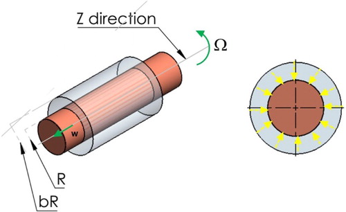
An analytical solution for steady-state problem of annular axisymmetric stagnation flow toward the moving cylinder for low and high Reynolds numbers has been extracted by Wang et al. [59]. Results of their analytical solution have been applied to the validation of numerical procedure employed in this paper. As can be seen in Figure 2, radiuses of inner and outer cylinders are R and bR respectively and the inner cylinder (shaft) has been enclosed by the outer cylinder (bushing).

Figure 2. Three-dimensional picture of axisymmetric stagnation flow on a cylinder.

2.1.4. Asymptotic solution for small Reynolds numbers

When W = 0 and Ω = 0, the following expansion in terms of small Reynolds number (Re << 1) has been applied to calculate dimensionless function f related to the radial velocity component. (14) $f=f_0+Re{f}_1+\cdots$(14) Analytical solution of zeroth-order and first-order equations [59] leads to the following relations for f₁ and f₀: (15) $f_0=\frac{\sqrt{b}[-2(b-1)\eta \ln \eta +\ln b.{\eta }^2+2(b-1-\ln b)\eta -(2b-2-\ln b\left)\right]}{(b-1)\left[2\right(b-1)-(b+1)\ln b]}$(15) (16) $\begin{array}{rl}{f}_1& =C_2+C_3\eta +C_4{\eta }^2+\left[288(-1+b{)}^{2}b{\eta }^2+72C_1(-1+b{)}^4\eta -108\right(-1+b)b\ln b.{\eta }^2\\ & +5(-1-b)b\ln b.{\eta }^3-72C_1(-1+b{)}^3(1+b)\ln b.\eta -6b{\ln }^{2}b.{\eta }^3+b{\ln }^{2}b.{\eta }^4\\ & +18C_1(-1+b^2){\ln }^{2}b.\eta -72(-1+b{)}^2\eta (3b\eta +C_1-2b{C}_1+b^2{C}_1)\ln \eta \\ & -6(-1+b)\ln b.\eta (-12b\eta +b{\eta }^2-12C_1+12b{C}_1+12b^2{C}_1-12b^3{C}_1)\ln \eta \\ & -18C_1(-1+b^2){\ln }^{2}b.\eta \ln \eta +36(-1+b{)}^{2}b(-\eta +{\eta }^2){\ln }^2\eta \\ & +18(-1+b)b\ln b.\eta {\ln }^2\eta \left]/\right[18(-1+b{)}^2(2-2b+(1+b)\ln b{)}^2]\end{array}$(16) Thus the boundary derivative f"(1) is fined analytically as below: (17) $f^{\mathrm{\prime }\mathrm{\prime }}\left(1\right)=\frac{2\sqrt{b}[\ln b-(b+1\left)\right]}{(b-1)\left[2\right(b-1)-(b+1)\ln b]}+Re{f}_1^{\mathrm{\prime }\mathrm{\prime }}\left(1\right)+O\left(R{e}^2\right)$(17) Comparison between the analytical and numerical results of f"(1) for Re = 0.1 and different values of b has been presented in Table 2.

Analytical solution of the steady energy equation when temperature at the wall is constant leads to the following dimension less function θ (η): (18) $\theta \left(\eta \right)=\frac{\underset{\eta }{\overset{b}{\int }}{\displaystyle \frac{1}{\chi }}exp\left(RePr.\underset{\chi }{\overset{b}{\int }}{\displaystyle \frac{f\left(t\right)}{t}}\text{d}t\right)\text{d}\chi }{\underset{1}{\overset{b}{\int }}{\displaystyle \frac{1}{\chi }}exp\left(RePr.\underset{\chi }{\overset{b}{\int }}{\displaystyle \frac{f\left(t\right)}{t}}\text{d}t\right)\text{d}\chi }$(18) By calculating dimensionless temperature gradient and heat flux at the wall, Nusselt number is expressed as follows: (19) $Nu=\frac{2R{q^{\mathrm{\prime }\mathrm{\prime }}}_w}{k(T_w-T_{\mathrm{\infty }})}=-4{\theta }^{\mathrm{\prime }}\left(1\right)$(19) Analytical and numerical results of Nusselt number for Re = 0.1 and different values of Prandtl number are reported in Table 3.

Table 2. Comparison of numerical and analytical results of f"(1).

	f"(1)
b	Analytical results	Numerical Results
1.1	650.352	650.475
2	11.001	11.012
10	0.6674	0.6687

Table 3. Analytical and numerical results of Nusselt number for Re = 0.1.

	b
	1.1		2
Pr	Analytical result	Numerical result	Analytical result	Numerical result
0.7	42.40	42.57	6.27	6.32
7	46.26	46.48	10.08	10.29
70	78.88	79.23	22.36	22.47
700	181.82	182.16	48.52	48.74

Table 4. Maximum and minimum values of the $|J_{ij}|$.

	$\left|J_{ij}\right|$
aqw(τ)/2k	Maximum value	Minimum value
Exponential	0.1718	3.2 × 10^−5
Sinus–cosines	0.1717	2.89 × 10^−5
Triangular	0.0884	7.50 × 10^−6
Trapezoidal	0.1595	5.06 × 10^−5

Table 5. Temperature history at point η₁ = 1.06 for exponential function of wall heat flux and S = −0.1.

τ	Exact temperature(°C)	Estimated temperature(°C)
0.1	82.3264	82.3223
0.2	86.4909	86.4918
0.3	91.4101	91.4119
0.4	97.1456	97.1467
0.5	103.7834	103.7826
0.6	111.4330	111.4307
0.7	120.2297	120.2276
0.8	130.3368	130.3368
0.9	141.9502	141.9526
1	155.3036	155.3052
1.1	170.6751	170.6712

2.2. Inverse problem

All inverse solutions for minimizing an objective function are based on an optimization method. One such method is the Levenberg–Marquardt algorithm which is an iterative method for solving nonlinear least squares problems of parameter estimation.

This algorithm is recommended for solving nonlinear parameter estimation problems. Also, it is used for ill-posed linear problems [60]. Therefore, it is used in this paper to the estimation of the unknown parameters of time-dependent heat flux.

The main steps of Levenberg–Marquardt inverse method are the sensitivity analysis, iteration process, convergence criterion and calculation algorithms as discussed below.

The inverse problem is the estimation of time variations of heat flux using the transient temperature values measured by a sensor. Thus $a{q}_w\left(\tau \right)/2k$ (in which a is the cylinder radius and k is the fluid thermal conductivity with known values) is unknown and time dependent whereas the transient temperature $Y\left(\tau \right)$ is the measured transient temperature in the sensor position within time interval $0\le \tau \le {\tau }_f$.

The measured temperatures in the sensor position at times ${\tau }_i,i=1,2,\dots ,I$ are used to estimate $a{q}_w\left(\tau \right)/2k$. To solve this inverse problem, we consider the unknown heat flux function $a{q}_w\left(\tau \right)/2k$ to be parameterized in the following general linear form: (20) $a{q}_w\left(\tau \right)/2k=\sum _{j=1}^{N}P{}_j{C}_j\left(\tau \right)$(20) where P_j are the unknown parameter and $C_j\left(\tau \right)$ are known trial functions, e.g. polynomials, spline, etc. with N parameters. For this inverse heat transfer problem, parameters P should be estimated. For this purpose, the differences between measured and calculated temperatures are formed as objective function to be minimized.

Several methods exist to develop an objective function, one of which is the least-square method as defined below [61]: (21) $S_p=\sum _{i=1}^I{[Y_i-T_i(P\left)\right]}^2$(21) where S_p is the sum of the squares error and hence the objective function. In order to solve this inverse heat transfer problem and estimate N unknown parameters $P_j,j=1,2,\dots ,N$, the objective function S_p should be minimized. In (21), $P^T=[P_1,P_2,\dots ,P_I]$ is the vector of unknown parameters. Also, $T_i\left(P\right)=T(P,{\tau }_i)$ and $Y_i=Y\left({\tau }_i\right)$ are the estimated and measured temperatures at time ${\tau }_i$, respectively. The estimated temperature $T_i\left(P\right)$ is obtained from solution of direct problem (9, 12) at the measurement (sensor) point using the unknown parameters $P_j,j=1,2,\dots ,N$.

2.2.1. Sensitivity analysis and calculation of the Jacobian matrix

Prior to solving the inverse problem, it is useful to analyse it and the estimated parameter’s sensitivities to unknown parameters. This analysis can yield a metric for best position of the temperature sensor and a criterion for the stability of the inverse solution. The sensitivity coefficients representing the estimated temperature sensitivity to small parameter variations are defined as (22). (22) $J_{ij}=\frac{T_i(P_1,P{}_2,\dots ,P_j+ϵP_j,\dots ,P_N)-T_i(P_1,P{}_2,\dots ,P_j,\dots ,P_N)}{ϵP_j}$(22) where $ϵ={10}^{-6}$.

The coefficients of (22) comprise the elements of the sensitivity matrix J. (23) $J\left(P\right)={\left[\frac{\mathrm{\partial }{T}^T\left(P\right)}{\mathrm{\partial }P}\right]}^T=\left[\begin{array}{cccc}\frac{\mathrm{\partial }{T}_1}{\mathrm{\partial }{P}_1}& \frac{\mathrm{\partial }{T}_1}{\mathrm{\partial }{P}_2}& \cdots & \frac{\mathrm{\partial }{T}_1}{\mathrm{\partial }{P}_N}\\ \frac{\mathrm{\partial }{T}_2}{\mathrm{\partial }{P}_1}& \frac{\mathrm{\partial }{T}_2}{\mathrm{\partial }{P}_2}& \cdots & \frac{\mathrm{\partial }{T}_2}{\mathrm{\partial }{P}_N}\\ ⋮& ⋮& \cdots & ⋮\\ \frac{\mathrm{\partial }{T}_I}{\mathrm{\partial }{P}_1}& \frac{\mathrm{\partial }{T}_I}{\mathrm{\partial }{P}_2}& \cdots & \frac{\mathrm{\partial }{T}_I}{\mathrm{\partial }{P}_N}\end{array}\right]$(23) In the above relation J actually is the Jacobian matrix.

where N and I are total number of unknown parameters and total number of measurements respectively that I ≥ N.

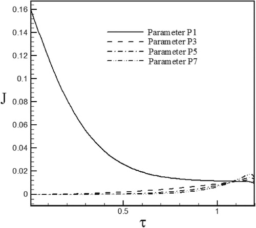
With small sensitivity coefficients, the inverse problem is so-called an ill-posed problem meaning that the inverse problem is sensitive to the measurement errors and an accurate estimation of the parameters cannot be achieved. Thus coefficients with high absolute values, leading to stable inverse analysis, are more desirable. Maximum and minimum values of $|J_{ij}|$ for the case of Re = 100 and S = 0.5 have been reported in Table 4 and the sensitivity coefficients for selected parameters have been plotted in Figures 3–6. The results show that in the initial times, the sensitivity to the P₁ parameter is lower compared to other parameters because it has a higher sensitivity coefficient and the sensitivity coefficient of other parameters is almost equal to zero this means that in the initial times the estimated parameters are not suitable for estimating unknown functions but in later times, the sensitivity coefficient of P₁decreases and in contrast, the sensitivity coefficient of other parameters increases and leads to convergence of iteration method.

Figure 3. Variations of sensitivity coefficient for estimation of the heat flux in the form of exponential function.

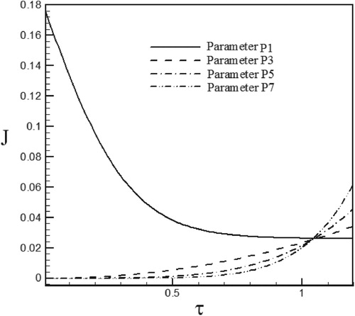
Figure 4. Variations of sensitivity coefficient for estimation of the heat flux in the form of sinus–cosines function.

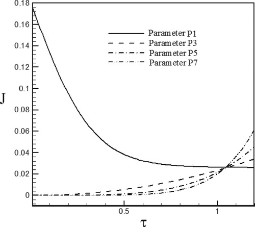
Figure 5. Variations of sensitivity coefficient for estimation of the heat flux in the form of triangular function.

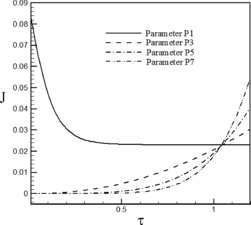
Figure 6. Variations of sensitivity coefficient for estimation of the heat flux in the form of trapezoidal function.

2.2.2. The iterative procedure

The sensitivity matrix is a nonlinear function of the vector of unknown parameters. Therefore, an iterative procedure is used to linearize the vector of estimated values. This process is carried out through Tailor series expansion around the current value $P^k$ at iteration k, as [62] (24) $P^{k+1}=P^k+[{\left(J^k\right)}^T{J}^k+{\mu }^k{\mathrm{\Omega }}^k{]}^{-1}(J^k{)}^T\left[Y-T\left(P^k\right)\right]$(24) whereμ^k is a positive scalar value named damping parameter and Ω^k is a diagonal matrix. ${\mu }^k{\mathrm{\Omega }}^k$ is the damping parameter matrix used to dampen the oscillations and instabilities resulting for the ill-conditioned character of the inverse problem. A large value is assumed for this parameter in the beginning of the iteration process because the problem is generally ill-posed around the initial guess chosen for the iteration process. This parameter can be far from the actual parameters. As a result, in the beginning of the iteration, the Levenberg–Marquardt method tends toward the steepest decent method in which a very small step is taken in the negative gradient direction. Then, as the iteration continues the value of ${\mu }^k$ is reduced making the Levenberg–Marquardt method performs similar to Newton–Gauss method.

2.2.3. Convergence criterion

In order to the convergence of Equation (24), a convergence criterion is needed to stop the iteration procedure of the Levenberg–Marquardt method. This criterion prevents the expansion of the measured errors and together with the iteration algorithm as a regularization technique, changes the inverse problem into a well conditioned problem. The following convergence criterion is used in this study: (25) $S\left(P^{k+1}\right)<{ϵ}_1$(25) where ${ϵ}_1$ is the selected tolerance for stopping the minimization process, as chosen by the user based on the distortion amount of the measured data. This criterion examines whether the objective function using the obtained solution is adequately minimized.

2.2.4. Computational algorithm

Assuming an initial guess of $P^0$ for the unknown parameter vector P and k = 0 and${\mu }_0=0.05$, Levenberg–Marquardt algorithm is summarized in following steps:

1. Solve the direct problem using the initial guess for $P^k$, i.e. the initial guess for wall heat flux and temperature, in order to obtain the temperature vector $T\left(P^k\right)=(T_1,\dots ,T_I)$.

2. Calculate $S\left(P^k\right)$ using Equation (21).

3. Calculate the sensitivity matrix $J^k$ defined by Equation (23) and diagonal matrix ${\mathrm{\Omega }}^k$ using the current $P^k$ values. To calculate the diagonal matrix ${\mathrm{\Omega }}^k$, use the following relation: (26) ${\mathrm{\Omega }}^k=diag\left[(J^k{)}^T{J}^k\right]$(26)

4. Solve the following linear system of algebraic equations, obtained from the iteration of (24). (27) $[(J^k{)}^T{J}^k+{\mu }^k{\mathrm{\Omega }}^k]\mathrm{\Delta }{P}^k=(J^k{)}^T[Y-T(P^k\left)\right]$(27)

5. Calculate the new estimation of $P^{k+1}$ as (28) $P^{k+1}=P^k+\mathrm{\Delta }{P}^k$(28)

6. Solve the direct problem using the new estimate $P^{k+1}$ and get the vector $T\left(P^{k+1}\right)$ and then calculate $S\left(P^{k+1}\right)$ using Equation (21).

7. If $S\left(P^{k+1}\right)\ge S\left(P^k\right)$, then substitute ${\mu }^k$ with $10{\mu }^k$ and return to step 4.

8. If $S\left(P^{k+1}\right)<S\left(P^k\right)$, accept the new estimate $P^{k+1}$ and substitute ${\mu }^k$ with $0.1{\mu }^k$.

9. Check the stopping criterion (25). Stop the iterative procedure if it is satisfied. Else, substitute k with k+1 and return to step 3.

3. Results

As shown in the previous section, the Levenberg–Marquardt method has been applied to estimate the unknown wall flux in stagnation region of the impinging flow on the circular cylinder. Since no information is available on the unknown boundary condition, ninth-order polynomial with unknown coefficients has been used for estimating wall heat flux. The aim of this study is to determine the unknown coefficients by curve fitting based on Levenberg–Marquardt algorithm.

Implicit Finite Difference method is used to discretize the governing equations. Time variable is assumed dimensionless and the time step is considered $\mathrm{\Delta }\tau =0.01$. In this study, using the measured temperature at a point, the boundary heat flux and boundary temperature are estimated and the noise data sensitivity is evaluated. Noisy data are generated using (29). The stability of the proposed approach against different noise levels is analysed with $\sigma =0.01T_{max}$ and $\sigma =0.03T_{max}$. (29) $Y\left({\tau }_i\right)=Y_{ex}\left({\tau }_i\right)+\omega \sigma$(29) In the above equation, $\sigma$ is the standard deviation of the measurement errors and $\omega$ is a random variable with normal distribution, zero mean and unitary standard deviation. For the present study, $-2.576\le \omega \le 2.576$. Also, for noisy data the relation ${ϵ}_1={\sigma }^2{\tau }_f$ is considered where ${\tau }_f$ is the final dimensionless time parameter. In order to evaluate the accuracy of the proposed algorithm, exponential, sinus–cosines, triangular and trapezoidal functions are examined for $\frac{a{q}_w\left(\tau \right)}{2k}$.

Detailed descriptions for the time-dependent wall heat flux are shown as follows: (30) $\begin{array}{rl}\frac{a{q}_w\left(\tau \right)}{2k}& =300e^{\tau }-55.5e^{2\tau }\end{array}$(30) (31) $\begin{array}{rl}\frac{a{q}_w\left(\tau \right)}{2k}& =10+300\sin \left(\tau \right)+150\cos \left(3\tau \right)\end{array}$(31) (32) $\begin{array}{rl}\frac{a{q}_w\left(\tau \right)}{2k}& =\left\{\begin{array}{l}200+300\tau \text{for}0<\tau \le 0.6\\ 497-200\tau \text{for}\tau >0.6\end{array}\right.\end{array}$(32) (33) $\begin{array}{rl}\frac{a{q}_w\left(\tau \right)}{2k}& =\left\{\begin{array}{l}150\text{for}0<\tau \le 0.2\\ 50+500\tau \text{for}0.2<\tau \le 0.4\\ 250\text{for}0.4<\tau \le 0.6\\ 550-500\tau \text{for}0.6<\tau \le 0.8\\ 150\text{for}\tau >0.8\end{array}\right.\end{array}$(33)

Also, temperature history at points η₁ is presented for the above values as well as the estimated values. Also temperature history at point η₁ for the case of S = −0.1 and different functions of time-dependent wall heat flux has been presented in Tables 5–8.

In Figures 7–30, the above functions are compared with the functions calculated using the inverse method in the selected values of Reynolds numbers, and then the inverse solutions have been presented with the noisy data.

Figure 7. Calculated Heat flux with Re = 100 and S = −0.6 vs. the exact heat flux in the form of an exponential function.

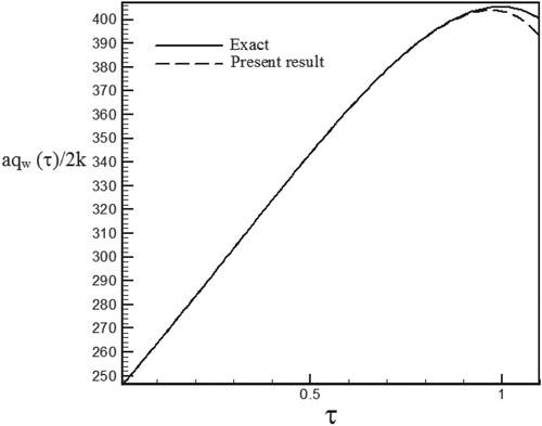
Figure 8. Temperature history at pointη₁ = 1.06 with Re = 100 and S = −0.6 for calculated heat flux vs. exact heat flux in the form of an exponential function.

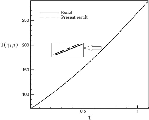
Figure 9. Calculated Heat flux with Re = 100 and S = −0.3 vs. the exact heat flux in the form of an exponential function.

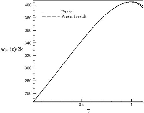
Figure 10. Temperature history at pointη₁ = 1.06 with Re = 100 and S = −0.3 for calculated heat flux vs. exact heat flux in the form of an exponential function.

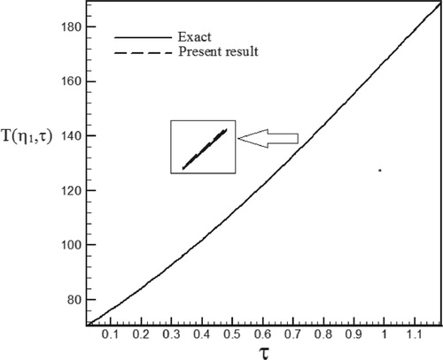
Figure 11. Calculated Heat flux with Re = 100 and S = 0.5 vs. the exact heat flux in the form of an exponential function.

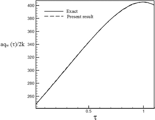
Figure 12. Temperature history at pointη₁ = 1.06 with Re = 100 and S = 0.5 for calculated heat flux vs. exact heat flux in the form of an exponential function.

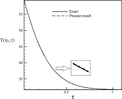
Figure 13. Calculated Heat flux with Re = 300 and S = −0.1 vs. the exact heat flux in the form of a sinus–cosines function.

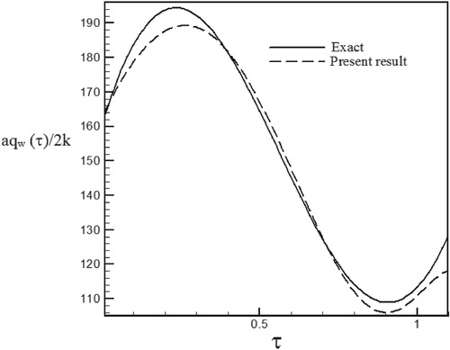
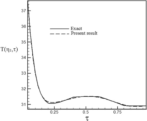
Figure 14. Temperature history at pointη₁ = 1.0225 with Re = 300 and S = −0.1 for calculated heat flux vs. exact heat flux in the form of a sinus–cosines function.

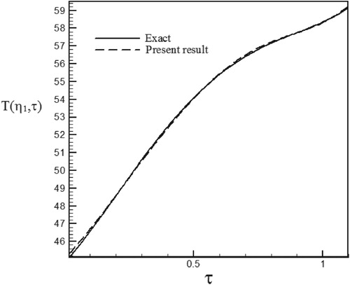
Figure 15. Calculated Heat flux with Re = 300 and S = 0.1 vs. the exact heat flux in the form of a sinus–cosines function.

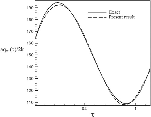
Figure 16. Temperature history at pointη₁ = 1.015 with Re = 300 and S = 0.1 for calculated heat flux vs. exact heat flux in the form of a sinus–cosines function.

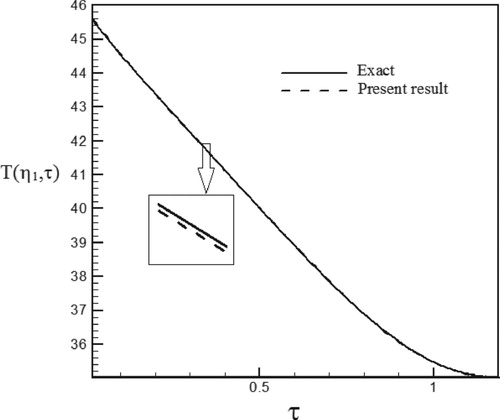
Figure 17. Calculated Heat flux with Re = 300 and S = 0.3 vs. the exact heat flux in the form of a sinus–cosines function.

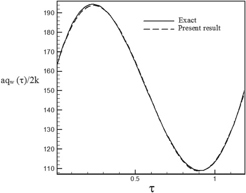
Figure 18. Temperature history at pointη₁ = 1.015 with Re = 300 and S = 0.3 for calculated heat flux vs. exact heat flux in the form of a sinus–cosines function.

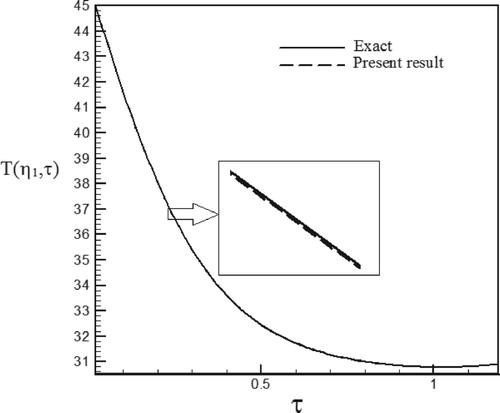
Figure 19. Calculated heat flux with Re = 200 and S = −0.1 vs. the exact heat flux in the form of a triangular function.

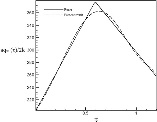
Figure 20. Temperature history at pointη₁ = 1.005 with Re = 200 and S = −0.1 for calculated heat flux vs. exact heat flux in the form of a triangular function.

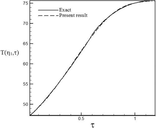
Figure 21. Calculated Heat flux with Re = 200 and S = 0.5 vs. the exact heat flux in the form of a triangular function.

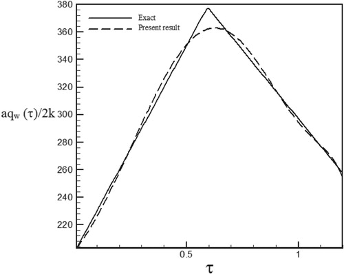
Figure 22. Temperature history at pointη₁ = 1.005 with Re = 200 and S = 0.5 for calculated heat flux vs. exact heat flux in the form of a triangular function.

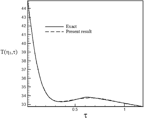
Figure 23. Calculated Heat flux with Re = 200 and S = 1 vs. the exact heat flux in the form of a triangular function.

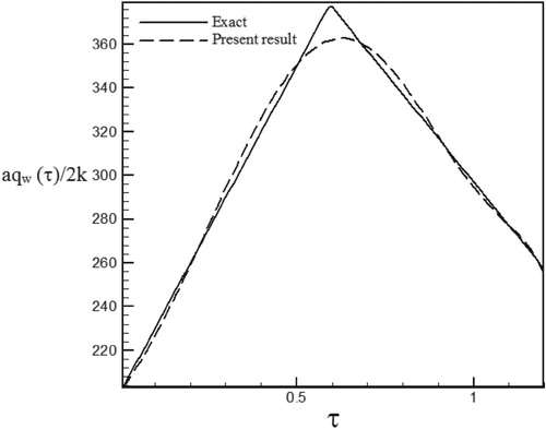
Figure 24. Temperature history at pointη₁ = 1.005 with Re = 200 and S = 1 for calculated heat flux vs. exact heat flux in the form of a triangular function.

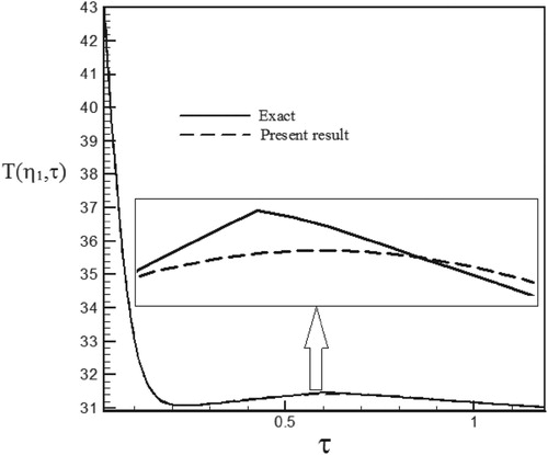
Figure 25. Calculated heat flux with Re = 150 and S = −0.1 vs. the exact heat flux in the form of a trapezoidal function.

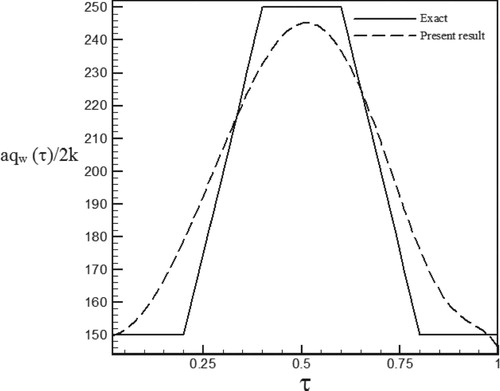
Figure 26. Temperature history at pointη₁ = 1.03 with Re = 150 and S = −0.1 for calculated heat flux vs. exact heat flux in the form of a trapezoidal function.

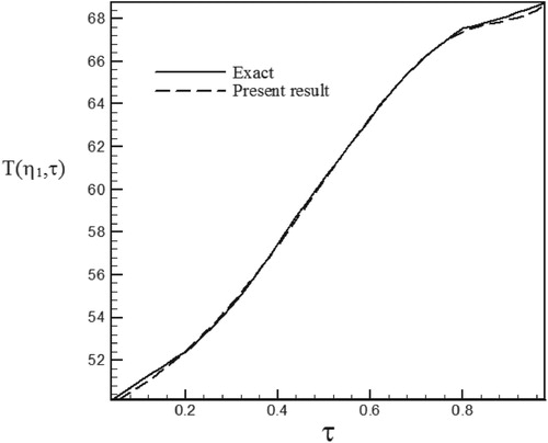
Figure 27. Calculated Heat flux with Re = 150 and S = 0.5 vs. the exact heat flux in the form of a trapezoidal function.

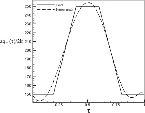
Figure 28. Temperature history at pointη₁ = 1.005 with Re = 150 and S = 0.5 for calculated heat flux vs. exact heat flux in the form of a trapezoidal function.

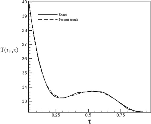
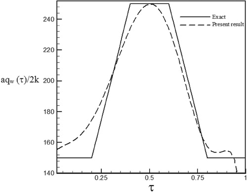
Figure 29. Calculated Heat flux with Re = 150 and S = 1 vs. the exact heat flux in the form of a trapezoidal function.

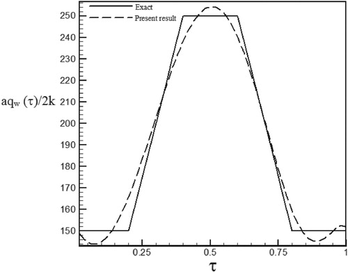
Figure 30. Temperature history at pointη₁ = 1.005 with Re = 150 and S = 1 for calculated heat flux vs. exact heat flux in the form of a trapezoidal function.

As can be seen, in cases estimated by triangular and trapezoidal functions, sharp corner points on the curves makes the estimation more difficult and increases the RMS error. In the case of suction at the wall (S > 0), by increasing the temperature gradient at the cylinder surface and decreasing the thermal boundary layer thickness, the rate of heat transfer is increased and the estimation of unknown functions becomes easier. But, as expected surface blowing (S < 0) acts completely reverse.

Different function form and various values of Reynolds numbers have been used to investigate of the stability and the accuracy of the solution method. Since our aim has been to examine different ranges of Reynolds numbers and surface transpiration rates we considered the different combination of Re and S. As can be seen in the figures related to temperature history, surface blowing causes more heat transfer from the hot wall to the fluid and increased the fluid temperature whereas surface suction absolutely acts vice versa and leads to a decrease in the fluid temperature.

Figure 31. Calculated heat flux with Re = 100 and S = −0.6 with noisy data (σ = 0.01T_max) vs. the exact heat flux in the form of an exponential function.

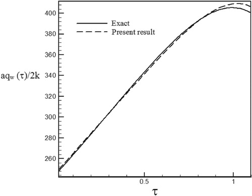
Figure 32. Calculated heat flux with Re = 100 and S = −0.6 with noisy data (σ = 0.03T_max) vs. the exact heat flux in the form of an exponential function.

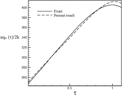
Figure 33. Calculated heat flux with Re = 100 and S = −0.3 with noisy data (σ = 0.01T_max) vs. the exact heat flux in the form of an exponential function.

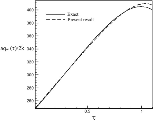
Figure 34. Calculated heat flux with Re = 100 and S = −0.3 with noisy data (σ = 0.03T_max) vs. the exact heat flux in the form of an exponential function.

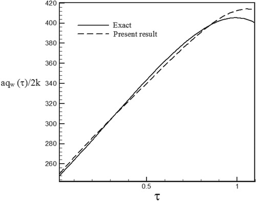
Figure 35. Calculated heat flux with Re = 100 and S = 0.5 with noisy data (σ = 0.01T_max) vs. the exact heat flux in the form of an exponential function.

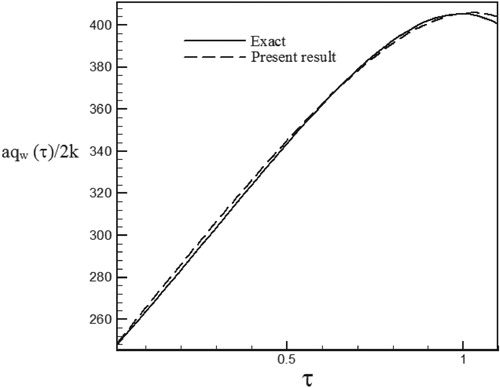
Figure 36. Calculated heat flux with Re = 100 and S = 0.5 with noisy data (σ = 0.03T_max) vs. the exact heat flux in the form of an exponential function.

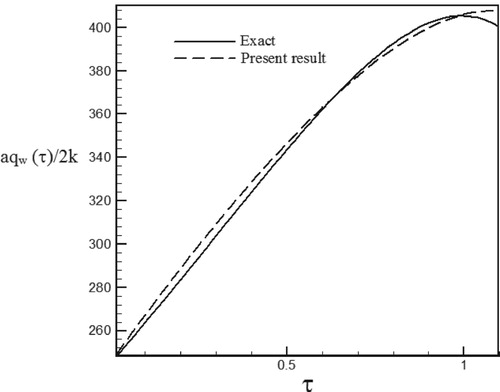
Figure 37. Calculated heat flux with Re = 300 and S = −0.1 with noisy data (σ = 0.01T_max) vs. the exact heat flux in the form of a sinus–cosines function.

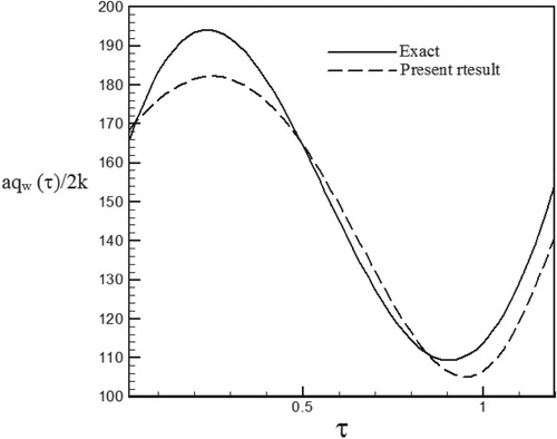
Figure 38. Calculated heat flux with Re = 300 and S = −0.1 with noisy data (σ = 0.03T_max) vs. the exact heat flux in the form of a sinus–cosines function.

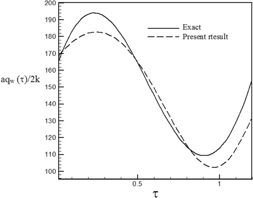
Figure 39. Calculated heat flux with Re = 300 and S = 0.1 with noisy data (σ = 0.01T_max) vs. the exact heat flux in the form of a sinus–cosines function.

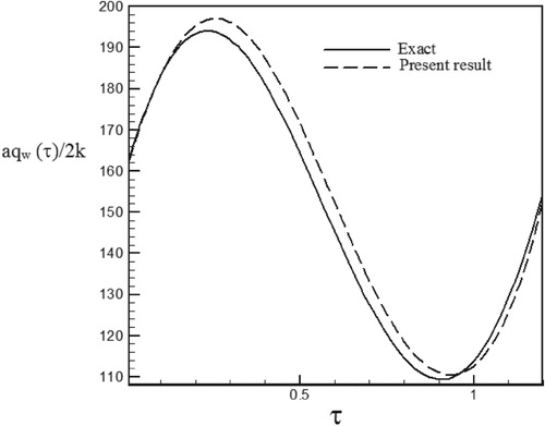
Figure 40. Calculated heat flux with Re = 300 and S = 0.1 with noisy data (σ = 0.03T_max) vs. the exact heat flux in the form of a sinus–cosines function.

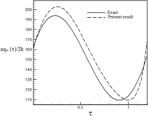
Figure 41. Calculated heat flux with Re = 300 and S = 0.3 with noisy data (σ = 0.01T_max) vs. the exact heat flux in the form of a sinus–cosines function.

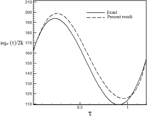
Figure 42. Calculated heat flux with Re = 300 and S = 0.3 with noisy data (σ = 0.03T_max) vs. the exact heat flux in the form of a sinus–cosines function.

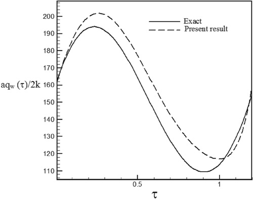
Figure 43. Calculated heat flux with Re = 200 and S = −0.1 with noisy data (σ = 0.01T_max) vs. the exact heat flux in the form of a triangular function.

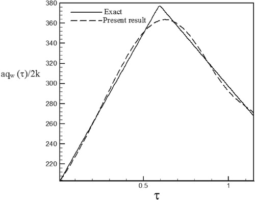
Figure 44. Calculated heat flux with Re = 200 and S = −0.1 with noisy data (σ = 0.03T_max) vs. the exact heat flux in the form of a triangular function.

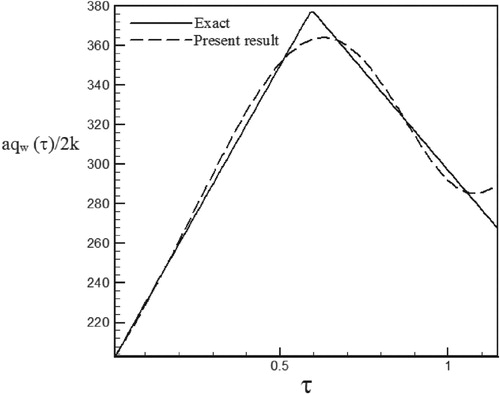
Figure 45. Calculated heat flux with Re = 200 and S = 0.5 with noisy data (σ = 0.01T_max) vs. the exact heat flux in the form of a triangular function.

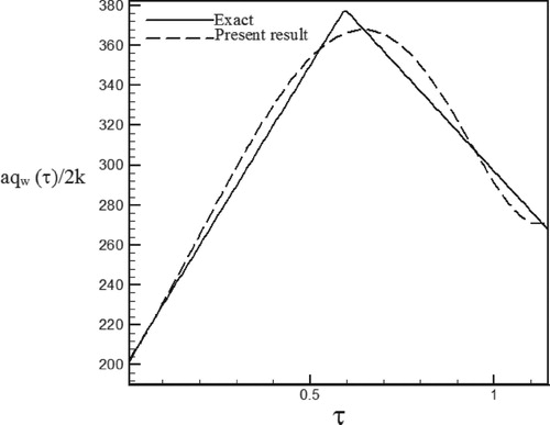
Figure 46. Calculated heat flux with Re = 200 and S = 0.5 with noisy data (σ = 0.03T_max) vs. the exact heat flux in the form of a triangular function.

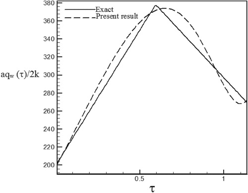
Figure 47. Calculated heat flux with Re = 200 and S = 1 with noisy data (σ = 0.01T_max) vs. the exact heat flux in the form of a triangular function.

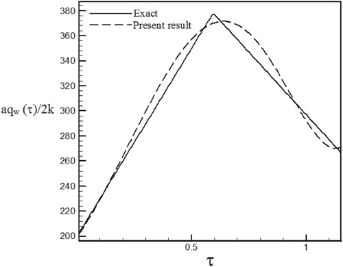
Figure 48. Calculated heat flux with Re = 200 and S = 1 with noisy data (σ = 0.03T_max) vs. the exact heat flux in the form of a triangular function.

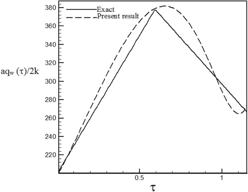
Figure 49. Calculated heat flux with Re = 150 and S = −0.1 with noisy data (σ = 0.01T_max) vs. the exact heat flux in the form of a trapezoidal function.

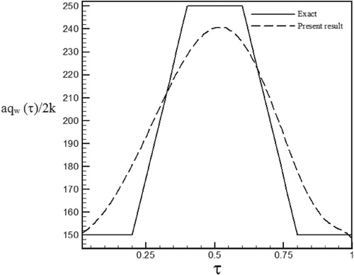
Figure 50. Calculated heat flux with Re = 150 and S = −0.1 with noisy data (σ = 0.03T_max) vs. the exact heat flux in the form of a trapezoidal function.

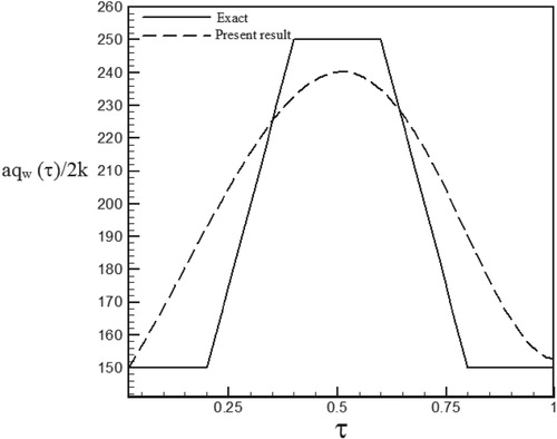
Figure 51. Calculated heat flux with Re = 150 and S = 0.5 with noisy data (σ = 0.01T_max) vs. the exact heat flux in the form of a trapezoidal function.

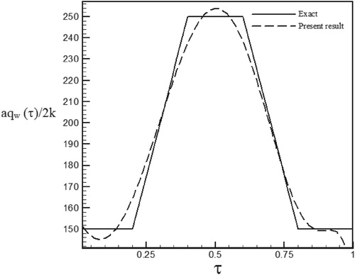
Figure 52. Calculated heat flux with Re = 150 and S = 0.5 with noisy data (σ = 0.03T_max) vs. the exact heat flux in the form of a trapezoidal function.

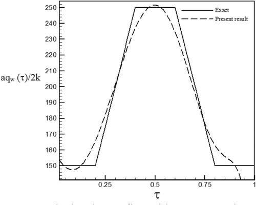
Figure 53. Calculated heat flux with Re = 150 and S = 1 with noisy data (σ = 0.01T_max) vs. the exact heat flux in the form of a trapezoidal function.

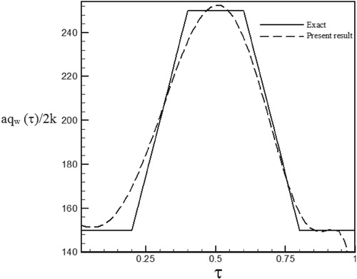
Figure 54. Calculated heat flux with Re = 150 and S = 1 with noisy data (σ = 0.03T_max) vs. the exact heat flux in the form of a trapezoidal function.

The root mean square (RMS) error, as a suitable measure for evaluating the accuracy of the Levenberg–Marquardt parameter estimation, is defined as follows: (34) $e_{RMS}=\sqrt{\frac{1}{I}\sum _{i=1}^I{\left[\frac{a{q}_w{\left({\tau }_i\right)}_{est}}{2k}-\frac{a{q}_w{\left({\tau }_i\right)}_{ex}}{2k}\right]}^2}$(34) where $\frac{a{q}_w{\left({\tau }_i\right)}_{est}}{2k}$ is the estimated function at time ${\tau }_i$, $\frac{a{q}_w{\left({\tau }_i\right)}_{ex}}{2k}$ is the exact function at time ${\tau }_i$ and I is the number of measurements. The RMS error is a measure to represent the difference between the estimated and actual function values. It is observed through the obtained results that the RMS error is the highest for trapezoidal function due to sharp corner points in the function curve. As witnessed in the following curves and tables as well as the calculated errors, the proposed approach is considered to have an acceptable accuracy.

The effect of noisy data on the time-dependent heat flux estimation is shown in Figures 31–54. The deviation of the estimated heat flux from the real wall heat flux increased when the standard deviation of measurement errors increased from σ = 0.01T_max to σ = 0.03T_max and as can be seen noisy data leads to more deviation of the obtained results compared to the exact data because according to the relation (29), noise in measured data by the sensor leads to error in relation (21).

Also, the RMS errors related to these results are given in Tables 9–12.

Table 6. Temperature history at point η₁ = 1.0225 for sinus–cosines function of wall heat flux and S=−0.1.

τ	Exact temperature (°C)	Estimated temperature (°C)
0.1	46.5274	46.7134
0.2	48.5330	48.5686
0.3	50.5463	50.4659
0.4	52.4117	52.2968
0.5	54.0286	53.9595
0.6	55.3476	55.3673
0.7	56.3649	56.4595
0.8	57.1211	57.2164
0.9	57.7163	57.7290
1	58.3223	58.2908
1.1	59.1481	59.2397

Table 7. Temperature history at point η₁ = 1.005 for triangular function of wall heat flux and S = −0.1.

τ	Exact temperature (°C)	Estimated temperature (°C)
0.1	49.3113	49.2427
0.2	52.3592	52.3006
0.3	55.7201	55.7634
0.4	59.3232	59.4951
0.5	63.1318	63.3086
0.6	67.2927	67.9537
0.7	70.3718	70.1495
0.8	72.5738	72.6426
0.9	74.1141	74.2854
1	75.0867	75.1158
1.1	75.5584	75.4294

Table 8. Temperature history at point η₁ = 1.03 for trapezoidal function of wall heat flux and S = −0.1.

τ	Exact temperature (°C)	Estimated temperature (°C)
0.1	50.9891	50.5880
0.2	52.3944	52.6362
0.3	54.3783	54.9982
0.4	57.2096	57.5645
0.5	60.2797	60.1976
0.6	63.0932	62.7306
0.7	65.4690	64.9810
0.8	66.8693	66.7747
0.9	67.9637	67.4946
1	68.2741	68.4681
1.1	69.1343	68.7815

Table 9. RMS error for exponential function of wall heat flux.

	eRMS
Dimensionless transpiration	σ = 0	σ = 0.01Tmax	σ = 0.03Tmax
S = −0.6	0.0102	0.142	0.289
S = −0.3	0.0057	0.138	0.281
S = 0.5	0.0024	0.102	0.248

Table 10. RMS error for sinus–cosines function of wall heat flux.

	eRMS
Dimensionless transpiration	σ = 0	σ = 0.01Tmax	σ = 0.03Tmax
S = −0.1	0.209	0.393	0.452
S = 0.1	0.091	0.112	0.241
S = 0.3	0.0043	0.185	0.293

Table 11. RMS error for triangular function of wall heat flux.

	eRMS
Dimensionless transpiration	σ = 0	σ = 0.01Tmax	σ = 0.03Tmax
S = −0.1	0.231	0.287	0.403
S = 0.5	0.218	0.304	0.448
S = 1	0.205	0.310	0.458

Table 12. RMS error for trapezoidal function of wall heat flux.

	eRMS
Dimensionless transpiration	σ = 0	σ = 0.01Tmax	σ = 0.03Tmax
S = −0.1	0.401	0.451	0.562
S = 0.5	0.346	0.387	0.492
S = 1	0.338	0.376	0.483

As can be seen in the tables, the error values for estimating triangular and trapezoidal functions are higher than exponential and sinus–cosines functions because of high gradient changes are not completely recovered by estimation function and some oscillations are observed near the singular points. We note that functions containing discontinuities and sharp comers (i.e. discontinuities on their first derivatives) are the most difficult to be recovered by an inverse analysis. Generally the results depend on the physical character of the problem, number of parameters to be estimated, initial guess, etc.

4. Conclusion

In this paper, a semi-similar solution to axisymmetric inverse problem based on the measured temperature distribution at a point in stagnation region of permeable wall, is presented to the estimation of time-dependent heat flux. In order to estimate the unknown boundary condition, ninth-order polynomials function with coefficients obtained by Levenberg–Marquardt parameter estimation algorithm has been used. The RMS error was calculated for different examples. The major results of this paper can be summarized as follows:

• — By comparing the sensitivity coefficients in S = 0.5 and Re = 100, it results that the maximum and minimum values of the sensitivity coefficients are 0.1718 and 7.50 × 10⁻⁶ respectively which is related to exponential and triangular heat flux. Therefore, the exponential heat flux shows the lowest sensitivity to the P_j parameters and the triangular heat flux has the highest sensitivity to these parameters.

• — The maximum RMS error values for σ = 0, σ = 0.01T_max and σ = 0.03Tmax are 0.401, 0.451 and 0.562, respectively, which were obtained to estimate the trapezoidal heat flux at S = −0.1. These results show that if there are non-derivative points in the unknown function, the accuracy of the parameter estimation method decreases.

• — In most cases, the RMS error increases with increasing the rate of surface blowing due to the removal of the thermal boundary layer from the surface.

• — Based on the studied cases and by comparing the obtained heat flux with the exact values and the fact that no prior data is required regarding the structure of the unknown function, and considering the acceptable stability against noisy data, it is concluded that this approach is an effective method for estimating of the time-dependent heat flux.

Nomenclature

a	=	Cylinder radius [m]
C	=	Known trial functions used in Levenberg–Marquardt method
Cp	=	Specific heat capacity [J kg−1K−1]
eRMS	=	Root mean square error
$f$	=	Dimensionless function defining velocity field
h	=	Convective heat transfer coefficient [W (m−2K−1]
$S$	=	Dimensionless transpiration
Sp	=	Sum of the square error
I	=	Number of measurements
J	=	Sensitivity matrix
$k$	=	Thermal conductivity [W (m−1K−1)]
$\overline{k}$	=	Free stream strain rate [1 s−1]
N	=	Number of unknown parameters
Nu	=	Nusselt number
$P$	=	Fluid pressure [N m−2]
$p$	=	Dimensionless pressure
Pk	=	Vector of unknown parameters at current iteration
$r,z$	=	Cylindrical coordinates [m]
Re	=	Reynolds number
T	=	Temperature [°C]
U0	=	Transpiration rate [m s−1]
$u$	=	Radial component of the velocity field [m s−1]
$w$	=	Axial component of the velocity field [m s−1]
$t$	=	Time [s]
$T_{}$	=	Free stream temperature [°C]
qw(t)	=	Time-dependent wall heat flux [W m−2]
Y	=	Measured transient temperature in the sensor position [°C]
$\eta$	=	Dimensionless radius
$\theta$	=	Dimensionless temperature
τ	=	Dimensionless time
$\mu$	=	Dynamic viscosity [(Ns) m−2]
${\mu }^k$	=	Damping parameter
$\upsilon$	=	Kinematic viscosity [m2 s−1]
ρ	=	Fluid density [kg m−3]
α	=	Fluid thermal diffusivity coefficient [m2 s−1]
$\sigma$	=	Standard deviation of measurement errors
${ϵ}_1$	=	Selected tolerance for stopping the minimization process

Abbreviations

ACGM	=	Adjoint conjugate gradient method
LBM	=	Lattice Boltzmann method
TDMA	=	Tri-diagonal matrix algorithm
IHTC	=	Interfacial heat transfer coefficient
RMS	=	Root mean square

Disclosure statement

No potential conflict of interest was reported by the authors.

Appendix

Numerical solution method

Before solving the third-order differential equation (9), a change of the variable is applied as below: $\xi =f^{\mathrm{\prime }}\to {\xi }^{\mathrm{\prime }}=f^{\mathrm{\prime }\mathrm{\prime }}\to {\xi }^{\mathrm{\prime }\mathrm{\prime }}=f^{\mathrm{\prime }{\mathrm{\prime }}^{\mathrm{\prime }}}$This formulation is necessary to eliminate the need for third-order difference and to obtain a tri-diagonal system of linear algebraic equations at further stage of the analysis.

The first step in solving the system of nonlinear ordinary differential equations (9) and (12) is to convert them into a system of quasi linear differential equations. $\frac{\mathrm{\partial }{\xi }^{(k+1)}}{\mathrm{\partial }\tau }+M_0{\xi }^{\mathrm{\prime }{\mathrm{\prime }}^{(k+1)}}+M_1{\xi }^{{\mathrm{\prime }}^{(k+1)}}+M_2{\xi }^{(k+1)}+M_3{f}^{\left(k\right)}=M_4$ $\frac{\mathrm{\partial }{\theta }^{(k+1)}}{\mathrm{\partial }\tau }+L_0{\theta }^{\mathrm{\prime }{\mathrm{\prime }}^{(k+1)}}+L_1{\theta }^{{\mathrm{\prime }}^{(k+1)}}+L_2{\theta }^{(k+1)}+L_3{f}^{(k+1)}=L_4$where $M_0=-\frac{\eta }{Re}$ $M_1=-\frac{1}{Re}-\frac{f^{\left(k\right)}}{Re}$ $M_2=2{\xi }^{\left(k\right)}$ $M_3=-\frac{{\xi }^{{\mathrm{\prime }}^{\left(k\right)}}}{Re}$ $M_4={{\xi }^2}^{\left(k\right)}-\frac{f^{\left(k\right)}}{Re}{\xi }^{{\mathrm{\prime }}^{\left(k\right)}}+1$ $L_0=-\frac{\eta }{RePr}$ $L_1=-\frac{1}{RePr}-f^{}$ $L_2=\frac{d{q}_w\left(\tau \right)/d\tau }{q_w\left(\tau \right)}$ $L_3=-{\theta }^{{\mathrm{\prime }}^{\left(k\right)}}$ $L_4=-f{\theta }^{{\mathrm{\prime }}^{\left(k\right)}}$

where k and k + 1 are the iteration indices.

In the numerical analysis, we replace the boundary conditions ${\xi }^{(k+1)}(\mathrm{\infty },\tau )=1$, ${\theta }^{(k+1)}(\mathrm{\infty },\tau )=0$ by ${\xi }^{(k+1)}({\eta }_e,\tau )=1$, ${\theta }^{(k+1)}({\eta }_e,\tau )=0$, where ${\eta }_e$ is a sufficiently large value of $\eta$.

Then, the problem has been written in a finite difference form. The interval $1\le \eta \le {\eta }_e$ has been divided into (N–1) equal intervals and denotes the values of the dependent variables at ${\eta }_i=1+(i-1)h$ with the subscript i (= 1, 2,  … , N) where $h=({\eta }_e-1)/(N-1)$. Substituting, as usual, the expressions ${\xi }^{\mathrm{\prime }\mathrm{\prime }}=\frac{{\xi }_{i+1}-2{\xi }_i+{\xi }_{i-1}}{h^2},{\xi }^{\mathrm{\prime }}=\frac{{\xi }_{i+1}-\xi {}_{i-1}}{2h},{\theta }^{\mathrm{\prime }\mathrm{\prime }}=\frac{{\theta }_{i+1}-2{\theta }_i+{\theta }_{i-1}}{h^2},{\theta }^{\mathrm{\prime }}=\frac{{\theta }_{i+1}-\theta {}_{i-1}}{2h}$ $\frac{\mathrm{\partial }{\xi }_i}{\mathrm{\partial }\tau }=\frac{{\xi }_i-{\xi }_i^{old}}{\mathrm{\Delta }\tau },\frac{\mathrm{\partial }{\theta }_i}{\mathrm{\partial }\tau }=\frac{{\theta }_i-{\theta }_i^{old}}{\mathrm{\Delta }\tau }$Into equations and using the boundary conditions, at every time step we obtain a system of linear algebraic equations in a tri-diagonal form: $A_{2,2}{\xi }_2^{(k+1)}+A_{2,3}{\xi }_3^{(k+1)}=C_2-A_{2,1}$ $A_{i,i-1}{\xi }_{i-1}^{(k+1)}+A_{i,i}{\xi }_i^{(k+1)}+A_{i,i+1}{\xi }_{i+1}^{(k+1)}=C_i(i=3,4,\dots ,N-2)$ $A_{N-1,N-2}{\xi }_{N-2}^{(k+1)}+A_{N-1,N-1}{\xi }_{N-1}^{(k+1)}=C_{N-1}-A_{N-1,N}$ $A_{2,2}^{\mathrm{\prime }}{\theta }_2^{(k+1)}+A_{2,3}^{\mathrm{\prime }}{\theta }_3^{(k+1)}=C_2^{\mathrm{\prime }}-A_{2,1}^{\mathrm{\prime }}$ $A_{i,i-1}^{\mathrm{\prime }}{\theta }_{i-1}^{(k+1)}+A_{i,i}^{\mathrm{\prime }}{\theta }_i^{(k+1)}+A_{i,i+1}^{\mathrm{\prime }}{\theta }_{i+1}^{(k+1)}=C_i^{\mathrm{\prime }}(i=3,4,\dots ,N-2)$ $A_{N-1,N-2}^{\mathrm{\prime }}{\theta }_{N-2}^{(k+1)}+A_{N-1,N-1}^{\mathrm{\prime }}{\theta }_{N-1}^{(k+1)}=C_{N-1}^{\mathrm{\prime }}-A_{N-1,N}^{\mathrm{\prime }}$

where $A_{i,i-1}=\frac{M_0}{h^2}-\frac{M_1}{2h}$ $A_{i,i}=\frac{1}{\mathrm{\Delta }\tau }-\frac{2M_0}{h^2}+M_2$ $A_{i,i+1}=\frac{M_0}{h^2}+\frac{M_1}{2h}$ $C_i=M_4+\frac{{\xi }_i^{\left(old\right)}}{\mathrm{\Delta }\tau }-M_3{f}_i^{\left(k\right)}$ $A_{i,i-1}^{\mathrm{\prime }}=\frac{L_0}{h^2}-\frac{L_1}{2h}$ $A_{i,i}^{\mathrm{\prime }}=\frac{1}{\mathrm{\Delta }\tau }-\frac{2L_0}{h^2}+L_2$ $A_{i,i+1}^{\mathrm{\prime }}=\frac{L_0}{h^2}+\frac{L_1}{2h}$ $C_i^{\mathrm{\prime }}=L_4+\frac{{\theta }_i^{\left(old\right)}}{\mathrm{\Delta }\tau }-L_3{f}_i$In the above relations, the superscript (old) represents the calculated value of $\xi$ and $\theta$ in the previous time step.

These systems are composed of (N–2) equations for (N–2) unknowns ${\xi }_i^{(k+1)},{\theta }_i^{(k+1)}$. It can be solved quite easily by usual sweeping method. Once all of ${\xi }_i^{(k+1)}$ are determined, $f_i^{(k+1)}$ are obtained from $\xi =f^{\mathrm{\prime }}$, namely: $f_i^{(k+1)}=\underset{1}{\overset{{\eta }_i}{\int }}{\xi }_i^{(k+1)}\text{d}\eta$executing a numerical integration. The values of ${\xi }_i^{(k+1)}$ and $f_i^{(k+1)}$ obtained here are used to replace ${\xi }_i^{\left(k\right)}$ and $f_i^{\left(k\right)}$ for the next cycle. The convergence is considered achieved if $|{\xi }_i^{(k+1)}-{\xi }_i^{\left(k\right)}|\le ϵ$ and $|{\theta }_i^{(k+1)}-{\theta }_i^{\left(k\right)}|\le ϵ$ for all points, where $ϵ$ is a prescribed accuracy criterion.

References

- Huang CH, Wang P. A three-dimensional inverse heat conduction problem in estimating surface heat flux by conjugate gradient method. Int J Heat Mass Transf. 1999;42(18):3387–3403.
- Shiguemori EH, Harter FP, Campos Velho HF, et al. Estimation of boundary condition in conduction heat transfer by neural networks. Tend Mate Apl Comput. 2002;3:189–195.
- Volle F, Maillet D, Gradeck M, et al. Practical application of inverse heat conduction for wall condition estimation on a rotating cylinder. Int J Heat Mass Transf. 2009;52:210–221.
- Golbahar Haghighi MR, Eghtesad M, Malekzadeh P, et al. Three-dimensional inverse transient heat transfer analysis of thick functionally graded plates. Energy Convers Manage. 2009;50:450–457.
- Su J, Neto A. Two dimensional inverse heat conduction problem of source strength estimation in cylindrical rods. Appl Math Model. 2001;25:861–872.
- Hsu PT. Estimating the boundary condition in a 3D inverse hyperbolic heat conduction problem. Appl Math Comput. 2006;177:453–464.
- Shi J, Wang J. Inverse problem of estimating space and time dependent hot surface heat flux in transient transpiration cooling process. Int J Therm Sci. 2009;48:1398–1404.
- Ling X, Atluril SN., stability analysis for inverse heat conduction problems. Comput Model Eng Sci. 2006;13(3):219–228.
- Jiang BH, Nguyen TH, Prud’homme M. Control of the boundary heat flux during the heating process of a solid material. Int Commun Heat Mass Transfer. 2005;32:728–738.
- Chen SG, Weng CI, Lin J. Inverse estimation of transient temperature distribution in the end quenching test. J Mater Process Technol. 1999;86:257–263.
- Plotkowski A, Krane MM. Use of inverse heat conduction models for estimation of transient surface heat flux in electroslag remelting. J Heat Transfer. 2015;137(3):031301.
- Hsu PT, Wang SG, Li TY. An inverse problem approach for estimating the wall heat flux in film wise condensation on a vertical surface with variable heat flux and body force convection. Appl Math Model. 2000;24:235–245.
- Khaniki HB, Karimian SMH. Determining the heat flux absorbed by satellite surfaces with temperature data. J Mech Sci Technol. 2014;28:2393–2398.
- Beck J, Black well B, St. Clair C. Inverse heat conduction. New York: J. Wiley; 1985.
- Liu FB. A hybrid method for the inverse heat transfer of estimating fluid thermal conductivity and heat capacity. Int J Therm Sci. 2011;50(5):718–724.
- Mohammadiun M, Rahimi AB, Khazaee I. Estimation of the time-dependent heat flux using temperature distribution at a point by conjugate gradient method. Int J Therm Sci. 2011;50:2443–2450.
- Tai BL, Stephenson DA, Shih AJ. An inverse heat transfer method for determining work piece temperature in minimum quantity lubrication deep hole drilling. J Manuf Sci Eng. 2012;134(2):021006.
- Rahimi AB, Mohammadiun M. Estimation of the strength of the time-dependent heat source using temperature distribution at a point in a three layer system. Int J Eng. 2012;25:343–351.
- Mohammadiun H, Molavi H, Talesh Bahrami HR, et al. Real-time evaluation of severe heat load over moving interface of decomposing composites. J Heat Transfer. 2012;134(11):111202.
- Mohammadiun M, Molavi H, Talesh Bahrami HR, et al. Application of sequential function specification method in heat flux monitoring of receding solid surfaces. Heat Transfer Eng. 2014;35(10):933–941.
- Wu TS, Lee HL, Chang WJ, et al. An inverse hyperbolic heat conduction problem in estimating pulse heat flux with a dual-phase-lag model. Int Commun Heat Mass Transfer. 2015;60:1–8.
- Bamdad K, Ashorynejad HR. Inverse analysis of a rectangular fin using the lattice Boltzmann method. Energy Convers Manage. 2015;97:290–297.
- Chen CK, Su CR. Inverse estimation for temperatures of outer surface and geometry of inner surface of furnace with two layer walls. Energy Convers Manage. 2008;49:301–310.
- Terzi A, Foudhil W, Harmand S, et al. Experimental investigation on the evaporation of a wet porous layer inside a vertical channel with resolution of the heat equation by inverse method. Energy Convers Manage. 2016;126:158–167.
- Hey J, Malloy AC, Martinez-Botas R, et al. Conjugate heat transfer analysis of an energy conversion device with an updated numerical model obtained through inverse identification. Energy Convers Manage. 2015;94:198–209.
- Panda S, Bhowmik A, Das R, et al. Application of homotopy analysis method and inverse solution of a rectangular wet fin. Energy Convers Manage. 2014;80:305–318.
- Panda S, Singla RK, Das R, et al. Identification of design parameters in a solar collector using inverse heat transfer analysis. Energy Convers Manage. 2014;88:27–39.
- Lee HL, Chang WJ, Chen WL, et al. Inverse heat transfer analysis of a functionally graded fin to estimate time-dependent base heat flux and temperature distributions. Energy Convers Manage. 2012;57:1–7.
- Zhang L, Li L, Ju H, et al. Inverse identification of interfacial heat transfer coefficient between the casting and metal mold using neural network. Energy Convers Manage. 2010;51:1898–1904.
- Hiemenz K. Die Grenzchicht an einem in den gleichformingen Flussigkeitsstrom eingetauchten geraden Kreiszylinder. Dingler,s Polytech J. 1911;326:391–393.
- Homann FZ. Der Einfluss grosser Zahighkeit bei der Strmung um den Zylinder und um die Kugel. Zeitschr Angew Math Mech. 1936;16:153–164.
- Howarth L. The boundary layer in three dimensional flow. Part II. The flow near a stagnation point. Philos Mag. 1951;42(7):1433–1440.
- Davey A. Boundary layer flow at a saddle point of attachment. J Fluid Mech. 1951;10(4):593–610.
- Wang C. Axisymmetric stagnation flow on a cylinder. Q Appl Math. 1974;32(2):207–213.
- Gorla RSR. Nonsimilar axisymmetric stagnation flow on a moving cylinder. Int J Eng Sci. 1978;16(6):397–400.
- Gorla RSR. Transient response behaviour of an axisymmetric stagnation flow on a circular cylinder due to time dependent free stream velocity. Int J Eng Sci. 1978;16(7):493–502.
- Gorla RSR. Heat transfer in axisymmetric stagnation flow on a cylinder. Appl Sci Res J. 1976;32(5):541–553.
- Gorla RSR. Unsteady viscous flow in the vicinity of an axisymmetric stagnation-point on a cylinder. Int J Eng Sci. 1979;17(1):87–93.
- Cunning GM, Davis AMJ, Weidman PD. Radial stagnation flow on a rotating cylinder with uniform transpiration. J Eng Math. 1998;33(2):113–128.
- Takhar HS, Chamkha AJ, Nath G. Unsteady axisymmetric stagnation-point flow of a viscous fluid on a cylinder. Int J Eng Sci. 1999;37(15):1943–1957.
- Saleh R, Rahimi AB. Axisymmetric stagnation-point flow and heat transfer of a viscous fluid on a moving cylinder with time- dependent axial velocity and uniform transpiration. J Fluids Eng. 2004;126(6):997–1005.
- Rahimi AB, Saleh R. Axisymmetric stagnation-point flow and heat transfer of a viscous fluid on a Rotating cylinder with time- dependent angular velocity and uniform transpiration. J Fluids Eng. 2007;129(1):107–115.
- Rahimi AB, Saleh R. Similarity solution of unaxisymmetric heat transfer in stagnation-point flow on a cylinder with simultaneous axial and rotational movements. J Heat Transfer. 2008;130(5):054502-1–054502-5.
- Abbasi AS, Rahimi AB. Non-axisymmetric three- dimensional stagnation-point flow and heat transfer on a flat plate. J Fluids Eng. 2009;131(7):074501.1–074501.5.
- Abbasi AS, Rahimi AB. Three-dimensional stagnation- point flow and heat transfer on a flat plate with transpiration. J Thermophys Heat Transfer. 2009;23(3):513–521.
- Abbasi AS, Rahimi AB, Niazmand H. Exact solution of three-dimensional unsteady stagnation flow on a heated plate. J Thermophys Heat Transfer. 2011;25(1):55–58.
- Abbasi AS, Rahimi AB. Investigation of two-dimensional stagnation-point flow and heat transfer impinging on a flat plate. J Heat Transfer. 2012;134(6):064501-1–064501-5.
- Mohammadiun H, Rahimi AB. Stagnation-point flow and heat transfer of a viscous, compressible fluid on a cylinder. J Thermo Physics Heat Transfer. 2012;26(3):494–502.
- Mohammadiun H, Rahimi AB, Kianifar A. Axisymmetric stagnation-point flow and heat transfer of a viscous compressible fluid on a cylinder with constant heat flux. Sci Iran B. 2013;20(1):185–194.
- Rahimi AB, Mohammadiun H, Mohammadiun M. Axisymmetric stagnation flow and heat transfer of a compressible fluid impinging on a cylinder moving axially. J Heat Transfer. 2016;138(2):022201-1–022201-9.
- Rahimi AB, Mohammadiun H, Mohammadiun M. Self-similar solution of radial stagnation point flow and heat transfer of a viscous, compressible fluid impinging on a rotating cylinder. Iran J Sci Technol Trans Mech Eng. 2019;43(1):S141–S153.
- Mohammadiun H, Amerian V, Mohammadiun M, et al. Similarity solution of axisymmetric stagnation-point flow and heat transfer of a nanofluid on a stationary cylinder with constant wall temperature. Iran J Sci Technol Trans Mech Eng. 2017;41:91–91.
- Mohammadiun H, Amerian V, Mohammadiun M, et al. Axisymmetric stagnation-point flow and heat transfer of nano-fluid impinging on a with constant wall heat flux. Thermal Sci. 2019;23(5B):3153–3164.
- Zahmatkesh R, Mohammadiun H, Mohammadiun M, et al. Investigation of entropy generation in nanofluid’s axisymmetric stagnation flow over a cylinder with constant wall temperature and uniform surface suction-blowing. Alexandria Eng J. 2019;54:1483–1498.
- Hassanien IA, El-Havary HM, Salama AA. Chebyshev solution of axisymmetric stagnation flow on a cylinder. Energy Convers Manage. 1996;37(1):67–76.
- Hassanien IA, Salama AA. Flow and heat transfer of a micropolar fluid in an axisymmetric stagnation flow on a cylinder. Energy Convers Manage. 1997;38(3):301–310.
- Hassanien IA. Chebyshev solution of stagnation point flow. Energy Convers Manage. 1997;38(9):839–845.
- Lin a JC, Lin TH. Structure and temperature distribution of a stagnation-point diesel spray premixed flame. Energy Convers Manage. 2005;46:2892–2906.
- Hong L, Wang CY. Annular axisymmetric stagnation flow on a moving cylinder. Int J Eng Sci. 2009;47:141–152.
- Ozicik MN, Orlande HRB. Inverse heat transfer fundamentals and application. New York: Taylor & Francis; 2000.
- Azimi A. Thermo-hydraulically simulation of thermal systems using inverse evaluation, PhD thesis, Sharif University of Technology. (2007) Tehran, Iran. (In Persian).
- Beck JV, Arnold KJ. Parameter estimation in engineering and science. New York: Wiley; 1977.