Time-dependent lowest term estimation in a 2D bioheat transfer problem with nonlocal and convective boundary conditions

ABSTRACT

A solution method for an inverse problem of determining the time-dependent lowest order coefficient of the 2D bioheat Pennes equation with nonlocal boundary conditions and total energy integral overdetermination condition recently appeared in literature is analysed and improved. Improvements include convective boundary condition into the model, the development of an accurate forward solver, accurate determination of total energy, and the proposal of a method for the numerical treatment of the inverse problem from noisy data. In the method, the 2D bioheat Pennes equation is solved by the method of lines based on a highly accurate pseudospectral approach, and sought coefficient values are estimated by the Levenberg–Marquardt method with the discrepancy principle as stopping rule. Numerical experiments are reported to illustrate effectiveness of the proposed method.

Keywords:

• 2D Pennes equation
• nonlocal boundary condition
• generalized Fourier method
• Chebyshev pseudospectral methods
• nonlinear least-squares problems
• Levenberg–Marquardt method

2010 Mathematics Subject Classification:

• 31A25

1. Introduction

In this paper, we consider an inverse boundary value problem (IBVP) associated with a 2D linear second-order parabolic partial differential equation under convective and nonlocal boundary conditions, assuming an integral energy overdetermination condition. The model is intended to describe the bioheat transfer process in a rectangular perfused living tissue by means of the so-called Pennes equation for the temperature U of the tissue [1–3], (1) $U_t=U_{xx}+U_{yy}-p\left(t\right)U(x,y,t)+f(x,y,t),(x,y,t)\in ]0,1[\times ]0,L[\times ]0,\mathcal{T}],$(1) with boundary conditions (2) $\begin{array}{rl}& U(0,y,t)=U(1,y,t),0\le y\le L,0\le t\le \mathcal{T},\end{array}$(2) (3) $\begin{array}{rl}& U_x(0,y,t)+\mu U(0,y,t)=0,0\le y\le L,0\le t\le \mathcal{T},\end{array}$(3) (4) $\begin{array}{rl}& U(x,0,t)=U(x,L,t)=0,0\le x\le 1,0\le t\le \mathcal{T},\end{array}$(4) and initial condition (5) $U(x,y,0)=\phi (x,y),(x,y)\in [0,1]\times [0,L].$(5) In the above model, the tissue is supposed to have thickness equals to L and width equals to 1; the upper skin is located at y = L and there is a wall between the tissue and an adjoint blood vessel at y = 0 (Figure 1). Equation (1(1) $U_t=U_{xx}+U_{yy}-p\left(t\right)U(x,y,t)+f(x,y,t),(x,y,t)\in ]0,1[\times ]0,L[\times ]0,\mathcal{T}],$(1) ) relies on the Fourier law for heat conduction assuming that the tissue is homogeneous and has isotropic thermal properties. The effects of the presence of the microcirculatory system are collectively accounted to avoid local anatomic issues so that all the blood perfusion information is concentrated in the term $p\left(t\right)U(x,y,t)$, where $p=p\left(t\right)$ is the so called blood perfusion coefficient [2–4]. Besides, the source term f accounts for the volumetric rate of external irradiation and metabolic heat. The convective boundary condition (3(3) $\begin{array}{rl}& U_x(0,y,t)+\mu U(0,y,t)=0,0\le y\le L,0\le t\le \mathcal{T},\end{array}$(3) ) attempts to simulate the heat transfer by convection between the boundary of the tissue at x = 0 and the external environment, which is supposed to be at zero temperature [5]. Assumption (4(4) $\begin{array}{rl}& U(x,0,t)=U(x,L,t)=0,0\le x\le 1,0\le t\le \mathcal{T},\end{array}$(4) ) means that the upper skin and the wall are kept at zero temperature; in turn, the nonlocal periodic boundary condition (2(2) $\begin{array}{rl}& U(0,y,t)=U(1,y,t),0\le y\le L,0\le t\le \mathcal{T},\end{array}$(2) ) states that the boundary of the tissue at x = 0 and x = 1 are kept at the same (unknown) temperature. Nonlocal boundary conditions are characterized by the specification of values of the solution or its derivatives on a fixed part of the boundary together with a relationship between these values and the values of the same functions on other internal or boundary manifolds [6,7]. They are often observed in connection with a bioheat transfer model describing the relation between tissue temperature and arterial blood perfusion [8,9]. Note that the case $\mu =0$ is the so called Ionkin boundary condition [10,11] that describes an insulated condition at x = 0. For other bioheat models with application in distinct scenarios the reader is referred to [5,12–16].

Figure 1. Domain for perfusion estimation.

For simplicity from here on, we will take L = 1 which does not loss generality (see Remark 2.1 in [17])). Let $\mathrm{\Omega }=]0,1[\times ]0,1[$ and ${\mathrm{\Omega }}_{\mathcal{T}}=\mathrm{\Omega }\times ]0,\mathcal{T}]$. We denote by $C[0,\mathcal{T}]$ the set of all continuous functions on $[0,\mathcal{T}]$ and by $C^1[0,\mathcal{T}]$ the set of all differentiable functions on $[0,\mathcal{T}]$. Also $\begin{array}{rl}& C^2\left(\overline{\mathrm{\Omega }}\right)=\{u:\overline{\mathrm{\Omega }}\to \mathbb{R}|u,u_{x_i}{u}_{x_i{x}_j}\mathrm{a}\mathrm{r}\mathrm{e}\mathrm{c}\mathrm{o}\mathrm{n}\mathrm{t}\mathrm{i}\mathrm{n}\mathrm{u}\mathrm{o}\mathrm{u}\mathrm{s}\mathrm{o}\mathrm{n}\overline{\mathrm{\Omega }},1\le i,j\le 2\},\\ & C^{2,1}\left(\overline{{\mathrm{\Omega }}_{\mathcal{T}}}\right)=\{u:\overline{{\mathrm{\Omega }}_{\mathcal{T}}}\to \mathbb{R}|u_t,u_{x_i{x}_j}\mathrm{a}\mathrm{r}\mathrm{e}\mathrm{c}\mathrm{o}\mathrm{n}\mathrm{t}\mathrm{i}\mathrm{n}\mathrm{u}\mathrm{o}\mathrm{u}\mathrm{s}\mathrm{o}\mathrm{n}\overline{{\mathrm{\Omega }}_{\mathcal{T}}},1\le i,j\le 2\},\\ & C^{2,0}\left(\overline{{\mathrm{\Omega }}_{\mathcal{T}}}\right)=\{u:\overline{{\mathrm{\Omega }}_{\mathcal{T}}}\to \mathbb{R}|u,u_{x_i{x}_j}\mathrm{a}\mathrm{r}\mathrm{e}\mathrm{c}\mathrm{o}\mathrm{n}\mathrm{t}\mathrm{i}\mathrm{n}\mathrm{u}\mathrm{o}\mathrm{u}\mathrm{s}\mathrm{o}\mathrm{n}\overline{{\mathrm{\Omega }}_{\mathcal{T}}},1\le i,j\le 2\}.\end{array}$In the definitions above, the overline symbol denotes the closure of a set.

The inverse problem investigated in this work consists of finding a pair $\{p,U\}\in C[0,\mathcal{T}]\times C^{2,1}\left(\overline{{\mathrm{\Omega }}_{\mathcal{T}}}\right)$ satisfying (1(1) $U_t=U_{xx}+U_{yy}-p\left(t\right)U(x,y,t)+f(x,y,t),(x,y,t)\in ]0,1[\times ]0,L[\times ]0,\mathcal{T}],$(1) )–(5(5) $U(x,y,0)=\phi (x,y),(x,y)\in [0,1]\times [0,L].$(5) ) as well as the total integral overdetermination condition (6) ${\int }_0^1{\int }_0^{1}U(x,y,t)\mathrm{d}x\mathrm{d}y=E\left(t\right),0\le t\le \mathcal{T},$(6) where $E\left(t\right)$ stands for thermal energy. In particular, motivated by practical problems, the main goal of the paper is to estimate the unknowns from noise corrupted discrete data ${\tilde{E}}_{\ell }=E\left(t_{\ell }\right)+{ϵ}_{\ell },\ell =1,\dots ,N$, measured at time steps $t_{\ell }$. Thus, the study presented in this work complements an approach reported in [11], where the reconstruction of the unknowns is based on exact data.

Techniques for inverse blood perfusion determination in one-dimensional (1D) case based on initial and classical boundary conditions (Dirichlet, Neumann, Robin) and additional classical measurements are found in [18] and references therein; related works including existence and uniqueness results are also found in [19–22]. On the other hand, determination of blood perfusion in 1D cases based on nonlocal or nonclassical initial/boundary conditions and integral overdetermination data can be found in [8,23–26]. Moreover, such type of inverse problems in multidimensional cases have been studied in [10,11,27–30]. A 2D bioheat transfer model which considers the coefficient p to be space-dependent and includes a given temperature on the upper skin, adiabatic conditions at left and right walls, and convective heat transfer between the tissue and an adjoint large blood vessel is studied both theoretically and numerically in [1,31]. Based on these studies, the inverse problem of estimating the space-dependent perfusion coefficient in this type of model is addressed in [32] using a method of lines coupled with a nonlinear minimization protocol based on the regularized Gauss–Newton method. Identification procedures based on well-recognized approximation methods are available in several places. For instance, identification strategies based on Trefftz method can be found in [13,14], finite differences are used in [11,29], and the boundary element method is employed in [15].

The goal of the present paper is to introduce a stable numerical reconstruction method for the time-dependent perfusion coefficient $p\left(t\right)$ satisfying (1(1) $U_t=U_{xx}+U_{yy}-p\left(t\right)U(x,y,t)+f(x,y,t),(x,y,t)\in ]0,1[\times ]0,L[\times ]0,\mathcal{T}],$(1) ) – (5(5) $U(x,y,0)=\phi (x,y),(x,y)\in [0,1]\times [0,L].$(5) ) under the condition (6(6) ${\int }_0^1{\int }_0^{1}U(x,y,t)\mathrm{d}x\mathrm{d}y=E\left(t\right),0\le t\le \mathcal{T},$(6) ). As in [17], where the authors deal with the one dimensional reconstruction problem, the forward problem is approached by means of the method of lines, where the spatial derivatives in (1(1) $U_t=U_{xx}+U_{yy}-p\left(t\right)U(x,y,t)+f(x,y,t),(x,y,t)\in ]0,1[\times ]0,L[\times ]0,\mathcal{T}],$(1) ) are discretized through a highly accurate Chebyshev pseudospectral (CPS) approach [33,34]. This procedure results in a semidiscrete model involving an ODE system with respect to the variable t, which is then solved by the Crank–Nicolson method. The reconstruction problem is posed as a minimization problem whereby approximations for $p\left(t\right)$ are obtained. To solve the minimization problem, the Levenberg–Marquardt method [35,36] in conjunction with the discrepancy principle as stopping rule is considered. Such an approach requires accurate approximations to energy values at each iteration, this is the reason why we use the Clenshaw–Curtis quadrature rule, which is based on the Chebyshev points as nodes [34, chapter 12].

The outline of the paper is the following. In Section 2, we discuss the well-posedness of the inverse reconstruction problem. In Section 3, the numerical scheme for the forward problem is addressed. In Section 4, we describe the estimation procedure. In Section 5, we present and justify the use of the Clenshaw–Curtis quadrature rule to evaluation of energy values. In Section 6, we present some numerical results. The paper ends with concluding remarks.

2. Mathematical background

In order to ensure global well-posedness of the inverse problem, we first use the generalized Fourier method to obtain a formal solution to (1(1) $U_t=U_{xx}+U_{yy}-p\left(t\right)U(x,y,t)+f(x,y,t),(x,y,t)\in ]0,1[\times ]0,L[\times ]0,\mathcal{T}],$(1) )–(5(5) $U(x,y,0)=\phi (x,y),(x,y)\in [0,1]\times [0,L].$(5) ) in series form. We follow the line of analysis reported in [10,11], which addresses the case $\mu =0$. Proceeding in this way, the first step is to consider the following 2D spectral problem for $\mu \ne 0$, (7) $\begin{array}{rl}& \frac{{\mathrm{\partial }}^{2}Z}{\mathrm{\partial }{x}^2}+\frac{{\mathrm{\partial }}^{2}Z}{\mathrm{\partial }{y}^2}+\sigma Z=0,0<x,y<1,\end{array}$(7) (8) $\begin{array}{rl}& Z(0,y)=Z(1,y),\frac{\mathrm{\partial }Z}{\mathrm{\partial }x}(0,y)+\mu Z(0,y)=0,0\le y\le 1,\end{array}$(8) (9) $\begin{array}{rl}& Z(x,0)=Z(x,1)=0,0\le x\le 1,\end{array}$(9) where σ is the separation parameter. Using the variable separation method, we look for solutions of the form (10) $Z(x,y)=X\left(x\right)V\left(y\right).$(10) Substitution of (10(10) $Z(x,y)=X\left(x\right)V\left(y\right).$(10) ) into (7(7) $\begin{array}{rl}& \frac{{\mathrm{\partial }}^{2}Z}{\mathrm{\partial }{x}^2}+\frac{{\mathrm{\partial }}^{2}Z}{\mathrm{\partial }{y}^2}+\sigma Z=0,0<x,y<1,\end{array}$(7) )–(9(9) $\begin{array}{rl}& Z(x,0)=Z(x,1)=0,0\le x\le 1,\end{array}$(9) ) yields the following Sturm–Liouville problems (11) $\begin{array}{rl}& V^{″}\left(y\right)+\lambda V\left(y\right)=0,0<y<1,V\left(0\right)=V\left(1\right)=0,\end{array}$(11) (12) $\begin{array}{rl}& X^{″}\left(x\right)+\gamma X\left(x\right)=0,0<x<1,X\left(0\right)=X\left(1\right),X^{\prime }\left(0\right)+\mu X\left(0\right)=1.\end{array}$(12) Problem (11(11) $\begin{array}{rl}& V^{″}\left(y\right)+\lambda V\left(y\right)=0,0<y<1,V\left(0\right)=V\left(1\right)=0,\end{array}$(11) ) is standard and has eigenvalues given by ${\lambda }_n=n^2{\pi }^2$ and respective eigenfunctions $V_n=\sin \left(n\pi y\right)$, $n=1,2,\dots$. On the other hand, (12(12) $\begin{array}{rl}& X^{″}\left(x\right)+\gamma X\left(x\right)=0,0<x<1,X\left(0\right)=X\left(1\right),X^{\prime }\left(0\right)+\mu X\left(0\right)=1.\end{array}$(12) ) requires a special treatment since it is associated with a nonself-adjoint type problem. However, it is not difficult to check [17,26] that the eigenvalues ${\gamma }_m$ are given by $\begin{array}{rl}{\gamma }_{2m}& =(2\pi m{)}^2,m=1,2,\dots ,\\ {\gamma }_{2m-1}& ={\varkappa }_m^2,m=1,2,\dots ,\\ {\gamma }_0& =\left\{\begin{array}{cc}{\varkappa }_0^2,& \mu <0,\\ -s_0^2,& \mu >0,\end{array}\right.\end{array}$where ${\varkappa }_m$, $m=1,2,\dots$, are monotone increasing positive solutions of the equation $\varkappa \sin \frac{\varkappa }{2}+\mu \cos \frac{\varkappa }{2}=0$for $\mu <0$ and $\mu >0$, respectively; in turn, $s_0$ is the unique positive solution of the nonlinear equation $e^s=1+\frac{2\mu }{s-\mu },\mu >0.$In addition, the system of eigenfunctions $X_m\left(x\right)$, $m=0,1,2,\dots$, is given by $\begin{array}{rl}{X}_{2m}\left(x\right)& =\cos \left(2\pi mx\right)-\frac{\mu }{2\pi m}\sin \left(2\pi mx\right),\\ X_{2m-1}\left(x\right)& =\cos \left({\varkappa }_{m}x\right)-\frac{\mu }{{\varkappa }_m}\sin \left({\varkappa }_{m}x\right),m=1,2,\dots ,\\ X_0\left(x\right)& =\left\{\begin{array}{ll}\cos {\varkappa }_{0}x-\frac{\mu }{{\varkappa }_0}\sin {\varkappa }_{0}x,& \mu <0,\\ \frac{s_0-\mu }{s_0+\mu }{e}^{s_{0}x}+e^{-s_{0}x},& \mu >0.\end{array}\right.\end{array}$

Now it is easy to check that the product $Z_{m,n}(x,y)=V_n\left(y\right)X_m\left(x\right)$, $n=1,2,\dots$, $m=0,1,2,\dots ,$ are eigenfunctions of the two dimensional spectral problem (7(7) $\begin{array}{rl}& \frac{{\mathrm{\partial }}^{2}Z}{\mathrm{\partial }{x}^2}+\frac{{\mathrm{\partial }}^{2}Z}{\mathrm{\partial }{y}^2}+\sigma Z=0,0<x,y<1,\end{array}$(7) )–(9(9) $\begin{array}{rl}& Z(x,0)=Z(x,1)=0,0\le x\le 1,\end{array}$(9) ) for the case $\mu \ne 0$. Also, it can be shown that $W_{m,n}(x,y)=V_n\left(y\right)Y_m\left(x\right)$, $n=1,2,\dots$, $m=0,1,2,\dots$, and $Z_{m,n}$ are biorthogonal in $L^2\left(\mathrm{\Omega }\right)$, where (13) $\begin{array}{r}\begin{array}{rl}& Y_0\left(x\right)=\left\{\begin{array}{ll}\frac{2{\varkappa }_0}{\mu ({\varkappa }_0^2+{\mu }^2-2\mu )}\left(({\varkappa }_0^2-{\mu }^2)\sin \left({\varkappa }_{0}x\right)+2\mu {\varkappa }_0\cos \left({\varkappa }_{0}x\right)\right),& \mu <0,\\ -\frac{s_0+\mu }{2\mu (s_0^2-{\mu }^2+2\mu )}\left((s_0-\mu {)}^2{e}^{s_{0}x}-(s_0+\mu {)}^2{e}^{-s_{0}x}\right),& \mu >0,\end{array}\right.\\ & Y_{2m}\left(x\right)=-\frac{4\pi m}{\mu }\sin (2\pi mx),m=1,2,\dots ,\\ & Y_{2m-1}\left(x\right)=\frac{2{\varkappa }_m}{\mu ({\varkappa }_m^2+{\mu }^2-2\mu )}\left(({\varkappa }_m^2-{\mu }^2)\sin \left({\varkappa }_{m}x\right)\right.\\ & +\left.2\mu {\varkappa }_m\cos \left({\varkappa }_{m}x\right)\right),m=1,2,\dots ,\end{array}\end{array}$(13) are eigenfunctions of adjoint spectral problem to (12(12) $\begin{array}{rl}& X^{″}\left(x\right)+\gamma X\left(x\right)=0,0<x<1,X\left(0\right)=X\left(1\right),X^{\prime }\left(0\right)+\mu X\left(0\right)=1.\end{array}$(12) ). The system of roots functions of (7(7) $\begin{array}{rl}& \frac{{\mathrm{\partial }}^{2}Z}{\mathrm{\partial }{x}^2}+\frac{{\mathrm{\partial }}^{2}Z}{\mathrm{\partial }{y}^2}+\sigma Z=0,0<x,y<1,\end{array}$(7) )–(9(9) $\begin{array}{rl}& Z(x,0)=Z(x,1)=0,0\le x\le 1,\end{array}$(9) ) is then given by $Z_{m,n}$ jointly with the system $W_{m,n}$ of root functions of the corresponding adjoint problem. This comes as no surprise since it is characteristic for 2D problems that the product of eigenfunctions of two 1D spectral problems becomes eigenfunction of a 2D spectral problem. However, note that the boundary condition in (11(11) $\begin{array}{rl}& V^{″}\left(y\right)+\lambda V\left(y\right)=0,0<y<1,V\left(0\right)=V\left(1\right)=0,\end{array}$(11) ) is self adjoint since it is a Dirichlet boundary condition, but the boundary condition in (12(12) $\begin{array}{rl}& X^{″}\left(x\right)+\gamma X\left(x\right)=0,0<x<1,X\left(0\right)=X\left(1\right),X^{\prime }\left(0\right)+\mu X\left(0\right)=1.\end{array}$(12) ) is not. They are regular (but not strongly regular) [37] and unlike the case of $\mu \ne 0$, for the case $\mu =0$, the eigenvalues of the auxiliary spectral problem are the zeros of multiplicity two of the characteristic determinant. The expansion theorem in terms of eigenfunctions for the problem with regular boundary conditions [37] is not applicable to the case $\mu =0$. In the case $\mu =0,$ the corresponding system of eigenfunctions and associated eigenfunctions is Riesz basis in $L^2(0,1)$ [7]. The spectral problem (12(12) $\begin{array}{rl}& X^{″}\left(x\right)+\gamma X\left(x\right)=0,0<x<1,X\left(0\right)=X\left(1\right),X^{\prime }\left(0\right)+\mu X\left(0\right)=1.\end{array}$(12) ) with the boundary conditions in the case $\mu \ne 0$ has the system of eigenfunctions which is a basis with parenthesis in $L^2(0,1)$, [11].

In addition, it is well known that the products of two orthonormal eigenfunctions corresponding of two 1D self adjoint boundary conditions are also an orthonormal basis in $L^2\left(\mathrm{\Omega }\right)$ [38], but generally it is not characteristic for other boundary conditions: Even if the eigenfunction of two 1D spectral problems generate bases, this may not happen with the products [39]. For this reason, the business property of the products $Z_{m,n}(x,y)=V_n\left(y\right)X_m\left(x\right)$, $n=1,2,\dots$, $m=0,1,2,\dots ,$ of eigenfunctions (11(11) $\begin{array}{rl}& V^{″}\left(y\right)+\lambda V\left(y\right)=0,0<y<1,V\left(0\right)=V\left(1\right)=0,\end{array}$(11) ) and (12(12) $\begin{array}{rl}& X^{″}\left(x\right)+\gamma X\left(x\right)=0,0<x<1,X\left(0\right)=X\left(1\right),X^{\prime }\left(0\right)+\mu X\left(0\right)=1.\end{array}$(12) ) in $L^2\left(\mathrm{\Omega }\right)$ has to be studied. However, this system is complete since $V_n\doteq V_n\left(y\right)$, $n=1,2,\dots$ is an orthogonal basis and $X_m\doteq X_m\left(x\right)$, $m=0,1,2,\dots$, is basis with parenthesis in $L^2(0,1)$ [38]. Then $Z_{m,n}\doteq Z_{m,n}(x,y)$ is also a basis with parentheses in $L^2\left(\mathrm{\Omega }\right)$, since for arbitrary $g\in L^2\left(\mathrm{\Omega }\right)$ the series $\sum _{m=1}^{\mathrm{\infty }}{g}_{m,0}{Z}_{m,0}(x,y)+\sum _{m,n=1}^{\mathrm{\infty }}\left[g_{m,2n-1}{Z}_{m,2n-1}(x,y)+g_{m,2n}{Z}_{m,2n}(x,y)\right]$converges in $L^2\left(\mathrm{\Omega }\right)$, where $g_{m,n}={\int }_0^1{\int }_0^{1}g(x,y)W_{m,n}(x,y)\mathrm{d}x\mathrm{d}y$.

In the case $\mu =0$, the system of eigenfunctions and associated eigenfunctions of problem (7(7) $\begin{array}{rl}& \frac{{\mathrm{\partial }}^{2}Z}{\mathrm{\partial }{x}^2}+\frac{{\mathrm{\partial }}^{2}Z}{\mathrm{\partial }{y}^2}+\sigma Z=0,0<x,y<1,\end{array}$(7) )–(9(9) $\begin{array}{rl}& Z(x,0)=Z(x,1)=0,0\le x\le 1,\end{array}$(9) ) has the form $\begin{array}{rl}{Z}_{0,n}(x,y)& =2\sqrt{2}\sin \left(\pi ny\right),Z_{2m-1,n}(x,y)=4\sqrt{2}\cos \left(2\pi mx\right)\sin \left(\pi ny\right),\\ Z_{2m,n}(x,y)& =4\sqrt{2}(1-x)\sin \left(2\pi mx\right)\sin \left(\pi ny\right),n,m=1,2,\dots ,\end{array}$whereas the system of eigenfunctions and associated eigenfunctions of the adjoint problem is given by $\begin{array}{rl}{W}_{0,n}(x,y)& =\sqrt{2}(1-x)\sin \left(\pi ny\right),W_{2m,n}(x,y)=\sqrt{2}\sin \left(2\pi mx\right)\sin \left(\pi ny\right),\\ W_{2m-1,n}(x,y)& =\sqrt{2}(1-x)\cos \left(2\pi mx\right)\sin \left(\pi ny\right),m,n=1,2,\dots .\end{array}$Then, the sequences $Z_{m,n}\doteq Z_{m,n}(x,y)$ and $W_{m,n}\doteq W_{m,n}(x,y)$ form a biorthogonal system of functions on $\overline{\mathrm{\Omega }}$. Besides, each of these sequence form a Riesz basis in $L^2\left(\mathrm{\Omega }\right)$ [7].

The solution $U\doteq U(x,y,t)$ of the forward problem (1(1) $U_t=U_{xx}+U_{yy}-p\left(t\right)U(x,y,t)+f(x,y,t),(x,y,t)\in ]0,1[\times ]0,L[\times ]0,\mathcal{T}],$(1) )–(5(5) $U(x,y,0)=\phi (x,y),(x,y)\in [0,1]\times [0,L].$(5) ) for arbitrary $(p,f,\phi )$ is then sought in Fourier series form in terms of $Z_{m,n}$. We will not enter into details here; instead, we refer the reader to [11]. The associated inverse problem can be addressed by means of such representation, taking into account the overdetermination condition (6(6) ${\int }_0^1{\int }_0^{1}U(x,y,t)\mathrm{d}x\mathrm{d}y=E\left(t\right),0\le t\le \mathcal{T},$(6) ) with $p\left(t\right)$ as unknown. Indeed, in this case, the inverse problem can be reformulated as a Volterra integral equation of the second kind with respect to $r\left(t\right)=e^{{\int }_0^{t}p\left(s\right)\mathrm{d}}$and whose solution depends on smoothness assumptions on the data. This leads to existence and uniqueness of the solutions for the inverse problem. More precisely, provided such r exists on $C^1[0,1]$, the coefficient p can be determined from the equation (14) $p\left(t\right)=\frac{r^{\prime }\left(t\right)}{r\left(t\right)}.$(14) As the details are quite similar to the proof of the case $\mu =0$ presented in [11], we omit the proof. However, for convenience of the reader the existence and uniqueness of solution to the inverse problem is stated below under the following assumptions on φ, f and E: $\left(A_1\right)\begin{array}{rl}\phi & \in C^2\left(\overline{\mathrm{\Omega }}\right),\\ \phi (0,y)& =\phi (1,y),\phi (x,0)=\phi (x,1)=0,{\phi }_x(0,y)+\mu \phi (0,y)=0,\\ & (x,y)\in \overline{\mathrm{\Omega }};\\ {\phi }_{0,2n-1}& >0,{\phi }_{2m,2n-1}\ge 0,m,n=1,2,\dots \mathrm{f}\mathrm{o}\mathrm{r}\mu \le 0,\\ {\phi }_{0,2n-1}& <0,{\phi }_{2m,2n-1}\le 0,m,n=1,2,\dots \mathrm{f}\mathrm{o}\mathrm{r}\mu >0\end{array}$with ${\phi }_{m,n}={\int }_0^1{\int }_0^1\phi (x,y)W_{m,n}(x,y)\mathrm{d}x\mathrm{d}y$, $\left(A_2\right)\begin{array}{rl}& f\in C^{2,0}\left(\overline{{\mathrm{\Omega }}_{\mathcal{T}}}\right),\\ & f(0,y,t)=f(1,y,t),f(x,0,t)=f(x,1,t)=0,(x,y,t)\in \overline{{\mathrm{\Omega }}_{\mathcal{T}}}\\ & f_{2m,2n-1}\left(t\right)\ge 0,m=0,1,\dots ;n=1,2,\dots \mathrm{f}\mathrm{o}\mathrm{r}\mu \le 0,\\ & f_{2m,2n-1}\le 0,m=0,1,\dots ;n=1,2,\dots \mathrm{f}\mathrm{o}\mathrm{r}\mu >0\end{array}$with $f_{m,n}\left(t\right)={\int }_0^1{\int }_0^{1}f(x,y,t)W_{m,n}(x,y)\mathrm{d}x\mathrm{d}y$, $\left(A_3\right)\begin{array}{rl}& E\doteq E\left(t\right)\in C^1[0,\mathcal{T}],E\left(0\right)={\int }_0^1{\int }_0^1\phi (x,y)\mathrm{d}x\mathrm{d}y,\\ & E\left(t\right)>0,\mathrm{\forall }t\in [0,\mathcal{T}].\end{array}$The main result on existence and uniqueness of the solution of the inverse problem (1(1) $U_t=U_{xx}+U_{yy}-p\left(t\right)U(x,y,t)+f(x,y,t),(x,y,t)\in ]0,1[\times ]0,L[\times ]0,\mathcal{T}],$(1) )–(6(6) ${\int }_0^1{\int }_0^{1}U(x,y,t)\mathrm{d}x\mathrm{d}y=E\left(t\right),0\le t\le \mathcal{T},$(6) ) is presented as follows.

Theorem 2.1

Under the conditions $\left(A_1\right)$ –$\left(A_3\right)$ the inverse problem  (1(1) $U_t=U_{xx}+U_{yy}-p\left(t\right)U(x,y,t)+f(x,y,t),(x,y,t)\in ]0,1[\times ]0,L[\times ]0,\mathcal{T}],$(1) )–(6(6) ${\int }_0^1{\int }_0^{1}U(x,y,t)\mathrm{d}x\mathrm{d}y=E\left(t\right),0\le t\le \mathcal{T},$(6) ) has a unique solution pair $\{p,U\}\in C[0,\mathcal{T}]\times C^{2,1}\left(\overline{{\mathrm{\Omega }}_{\mathcal{T}}}\right)$ and this solution depends continuously upon the data $\{f,\phi ,E\}$.

Theorem 2.1 states that the inverse problem under investigation is well-posed in appropriate spaces of regular input data functions. However, in practice, the input data are inaccurate and the energy E is not smooth. Hence the solution of the inverse problem based on numerical differentiation following (14(14) $p\left(t\right)=\frac{r^{\prime }\left(t\right)}{r\left(t\right)}.$(14) ) as done in various papers, see, e.g. [8,11,29], becomes unstable and the calculated coefficient p loses its physical significance. This motivates the inverse problem method to be presented in Section 4 based on discrete data and the CPS collocation method.

3. Highly accurate forward solver

In this section, we will derive an efficient numerical approach for solving the bioheat model (1(1) $U_t=U_{xx}+U_{yy}-p\left(t\right)U(x,y,t)+f(x,y,t),(x,y,t)\in ]0,1[\times ]0,L[\times ]0,\mathcal{T}],$(1) )–(5(5) $U(x,y,0)=\phi (x,y),(x,y)\in [0,1]\times [0,L].$(5) ) that we will use in the numerical treatment of the inverse problem of interest. For this purpose, we will use the CPS method in which the discretization of spatial derivatives is done using the Chebyshev differentiation matrix, giving rise to a system of time-dependent ordinary differential equations that can be solved in in different ways. For the sake of clarity, before describing details of the proposed approach, let us introduce some generalities and notation about Chebyshev's differentiation matrix. Let $\mathsf{v}$ denote a vector with function values $v_i=v\left({\overline{x}}_i\right)$ as entries, where ${\overline{x}}_i$ are the so called Chebyshev nodes (also known as Chebyshev–Gauss–Lobatto nodes) within the interval $[-1,1]$, (15) ${\overline{x}}_i=\cos \frac{\pi i}{n},i=0,\dots ,n,n\ge 1,$(15) and let the associated $(n+1)\times (n+1)$ Chebyshev differentiation matrix be denoted by D. Assuming that the rows and columns of D are indexed from 0 to n, the entries of D are given by [34] (16) $\begin{array}{rl}& (D{)}_{00}=-(D{)}_{nn}=\frac{2n^2+1}{6},\\ & (D{)}_{jj}=\frac{-{\overline{x}}_j}{2(1-{\overline{x}}_j^2)},j=1,\dots ,n-1,\\ & (D{)}_{ij}=\frac{c_i}{c_j}\frac{(-1{)}^{i+j}}{({\overline{x}}_i-{\overline{x}}_j)},i\ne j,i,j=1,\dots ,n-1,\end{array}$(16) where $c_i=2$ if i = 0 or i = n and $c_i=1$ otherwise. Provided v is sufficiently smooth, it is well known that matrix D yields highly accurate approximations to $v^{\prime }\left({\overline{x}}_i\right)$, $v^{″}\left({\overline{x}}_i\right),\dots$, simply by taking $v^{\mathrm{\prime }}\left({\overline{x}}_i\right)\approx (D\mathsf{v}{)}_i$, $v^{″}\left({\overline{x}}_i\right)\approx (D^2\mathsf{v}{)}_i$, and so on [33,34]. Further, to approximate the derivative $v^{\prime }$ at Chebyshev nodes $x_i$ distributed within an interval $[a,b]$, observe that introducing the change of variable $x=x\left(\overline{x}\right)=a+\frac{b-a}{2}(\overline{x}+1)$, $\overline{x}\in [-1,1]$, and setting $u\left(\overline{x}\right)=v\left(x\right(\overline{x}\left)\right)$, we have $v^{\prime }\left(x\right)=\frac{2}{b-a}{u}^{\prime }\left(\overline{x}\right)$. This implies that the Chebyshev differentiation matrix with nodes within $[a,b]$ is simply $\frac{2}{b-a}$ times matrix D defined in (16(16) $\begin{array}{rl}& (D{)}_{00}=-(D{)}_{nn}=\frac{2n^2+1}{6},\\ & (D{)}_{jj}=\frac{-{\overline{x}}_j}{2(1-{\overline{x}}_j^2)},j=1,\dots ,n-1,\\ & (D{)}_{ij}=\frac{c_i}{c_j}\frac{(-1{)}^{i+j}}{({\overline{x}}_i-{\overline{x}}_j)},i\ne j,i,j=1,\dots ,n-1,\end{array}$(16) ).

With regard to the discretization of the bioheat problem, for simplicity we will consider a mesh consisting of $(n+1)\times (n+1)$ grid points on the unit square based on $(n+1)$ Chebyshev points within $[0,1]$ in each direction: (17) $x_i=\frac{1}{2}\left(1-\cos \frac{\pi i}{n}\right),y_j=\frac{1}{2}\left(1-\cos \frac{\pi j}{n}\right),0\le i,j\le n,$(17) and assume that grid points are numbered in lexicographic ordering. As the standard differentiation matrix is no longer used in this work, to discretize spatial derivatives, assume that the Chebyshev differentiation matrix with nodes within $[0,1]$ is also denoted by D and partitioned as (18) $D=[d_0,\dots ,d_n]=\left[\begin{array}{c}{r}_0^T\\ ⋮\\ r_n^T\end{array}\right],d_i,r_i\in {\mathbb{R}}^{n+1},$(18) where the subscript $\mathrm{T}$ stands for transpose of a vector or matrix. For future use, let ${\hat{d}}_i$, ${\breve{d}}_i$ denote the vectors formed by the first and last n components of $d_i$, respectively. Also, set (19) $D_1=[d_1,\dots ,d_n],R_1=\left[\begin{array}{c}{r}_1^T\\ ⋮\\ r_n^T\end{array}\right]=[{\breve{d}}_0,\dots ,{\breve{d}}_n].$(19) Then second-order partial derivatives with respect to x on the grid can be approximated as (20) $\begin{array}{rl}\left[\begin{array}{c}{U}_{xx}(x_0,y_j,t)\\ ⋮\\ U_{xx}(x_n,y_j,t)\end{array}\right]& \approx D\left[\begin{array}{c}{U}_x(x_0,y_j,t)\\ ⋮\\ U_x(x_n,y_j,t)\end{array}\right]=\sum _{i=0}^n{d}_i{U}_x(x_i,y_j,t)\\ & =-\mu U(x_0,y_j,t)d_0+\sum _{i=1}^n{d}_i{U}_x(x_i,y_j,t)\end{array}$(20) where the last equality is by virtue of (3(3) $\begin{array}{rl}& U_x(0,y,t)+\mu U(0,y,t)=0,0\le y\le L,0\le t\le \mathcal{T},\end{array}$(3) ). Now noting that $U_x(x_i,y_j,t)\approx r_i^T\left[\begin{array}{c}U(x_0,y_j,t)\\ ⋮\\ U(x_n,y_j,t)\end{array}\right],$using (20(20) $\begin{array}{rl}\left[\begin{array}{c}{U}_{xx}(x_0,y_j,t)\\ ⋮\\ U_{xx}(x_n,y_j,t)\end{array}\right]& \approx D\left[\begin{array}{c}{U}_x(x_0,y_j,t)\\ ⋮\\ U_x(x_n,y_j,t)\end{array}\right]=\sum _{i=0}^n{d}_i{U}_x(x_i,y_j,t)\\ & =-\mu U(x_0,y_j,t)d_0+\sum _{i=1}^n{d}_i{U}_x(x_i,y_j,t)\end{array}$(20) ) and the boundary condition (2(2) $\begin{array}{rl}& U(0,y,t)=U(1,y,t),0\le y\le L,0\le t\le \mathcal{T},\end{array}$(2) ), the approximation becomes $\begin{array}{rl}\left[\begin{array}{c}{U}_{xx}(x_0,y_j,t)\\ ⋮\\ U_{xx}(x_n,y_j,t)\end{array}\right]& \approx D_1{R}_1\left[\begin{array}{c}U(x_0,y_j,t)\\ ⋮\\ U(x_n,y_j,t)\end{array}\right]-\mu d_{0}U(x_0,y_j,t)\\ & =D_1\left[{\breve{R}}_1{U}^j+{\breve{d}}_{n}U(x_0,y_j,t)\right]-\mu d_{0}U(x_0,y_j,t),\end{array}$where (21) $\begin{array}{r}{\breve{R}}_1=[{\breve{d}}_0,\dots {\breve{d}}_{n-1}],\mathrm{a}\mathrm{n}\mathrm{d}{U}^j=\left[U\right(x_0,y_j,t),\dots ,U(x_{n-1},y_j,t){]}^T,j=0,1,\dots .\end{array}$(21) Since only unknowns $U(x_0,y_j,t),\dots ,U(x_{n-1},y_j,t)$ matter, with $e_1$ denoting the first canonical vector of ${\mathbb{R}}^n$, we conclude that (22) $\left[\begin{array}{c}{U}_{xx}(x_0,y_j,t)\\ ⋮\\ U_{xx}(x_{n-1},y_j,t)\end{array}\right]\approx \left({\hat{D}}_1\left[{\breve{R}}_1+{\breve{d}}_n{e}_1^T\right]-\mu {\hat{d}}_n{e}_1^T\right)U^j,j=0,1,\dots ,$(22) where we have introduced ${\hat{D}}_1=[{\hat{d}}_1,\dots ,{\hat{d}}_n].$ Therefore, an approximation to second-order derivatives with respect to x, for grid points associated to the unknowns only, can be written as follows: (23) $\left[\begin{array}{c}{U}_{xx}(x_0,y_1,t)\\ ⋮\\ U_{xx}(x_{n-1},y_1,t)\\ ⋮\\ U_{xx}(x_0,y_{n-1},t)\\ ⋮\\ U_{xx}(x_{n-1},y_{n-1},t)\end{array}\right]\approx I_{n-1}\otimes \left[{\hat{D}}_1\left({\breve{R}}_1+{\breve{d}}_n{e}_1^T\right)-\mu {\hat{d}}_n{e}_1^T\right]\left[\begin{array}{c}{U}^1\\ ⋮\\ U^{n-1}\end{array}\right],$(23) where ⊗ denotes Kronecker product and $I_M$ denotes the $M\times M$ identity matrix. A similar approximation for second-order derivatives with respect to y on the whole grid can readily be written. In fact, if we use Matlab notation and introduce $D_2=D(:,2:n),R_2=D(2:n,:),$ we deduce that (24) $\left[\begin{array}{c}{U}_{yy}(x_0,y_1,t)\\ ⋮\\ U_{yy}(x_{n-1},y_1,t)\\ ⋮\\ U_{yy}(x_0,y_{n-1},t)\\ ⋮\\ U_{yy}(x_{n-1},y_{n-1},t)\end{array}\right]\approx R_2{D}_2\otimes I_n\left[\begin{array}{c}{U}^1\\ ⋮\\ U^{n-1}\end{array}\right].$(24) Neglecting approximation errors, combination of (23(23) $\left[\begin{array}{c}{U}_{xx}(x_0,y_1,t)\\ ⋮\\ U_{xx}(x_{n-1},y_1,t)\\ ⋮\\ U_{xx}(x_0,y_{n-1},t)\\ ⋮\\ U_{xx}(x_{n-1},y_{n-1},t)\end{array}\right]\approx I_{n-1}\otimes \left[{\hat{D}}_1\left({\breve{R}}_1+{\breve{d}}_n{e}_1^T\right)-\mu {\hat{d}}_n{e}_1^T\right]\left[\begin{array}{c}{U}^1\\ ⋮\\ U^{n-1}\end{array}\right],$(23) ) and (24(24) $\left[\begin{array}{c}{U}_{yy}(x_0,y_1,t)\\ ⋮\\ U_{yy}(x_{n-1},y_1,t)\\ ⋮\\ U_{yy}(x_0,y_{n-1},t)\\ ⋮\\ U_{yy}(x_{n-1},y_{n-1},t)\end{array}\right]\approx R_2{D}_2\otimes I_n\left[\begin{array}{c}{U}^1\\ ⋮\\ U^{n-1}\end{array}\right].$(24) ) together with the collocation method yield a semidiscrete model described as (25) $\begin{array}{rl}{W}^{\prime }\left(t\right)& =G(t,W),t>0,\\ W\left(0\right)& =U_0,\end{array}$(25) where $W\left(t\right)$ is a long vector containing block component $U^1,\dots ,U^{n-1}$, (26) $G(t,W)=[I_{n-1}\otimes [{\hat{D}}_1({\breve{R}}_1+{\breve{d}}_n{e}_1^T)-\mu {\hat{d}}_n{e}_1^T]+R_2{D}_2\otimes I_n-p(t\left)I\right]W+S\left(t\right)$(26) with I denoting the identity matrix of appropriate order, (27) $S\left(t\right)=\left[f\right(x_0,y_0,t),\dots ,f(x_{n-1},y_0,t),\dots ,f(x_0,y_n,t),\dots ,f(x_{n-1},y_n,t){]}^{\mathrm{T}}$(27) and $U_0=\left[\phi \right(x_0,y_0),\dots ,\phi (x_{n-1},y_0),\dots ,\phi (x_0,y_n),\dots ,\phi (x_{n-1},y_n){]}^{\mathrm{T}}.$The initial value problem (IVP) (25(25) $\begin{array}{rl}{W}^{\prime }\left(t\right)& =G(t,W),t>0,\\ W\left(0\right)& =U_0,\end{array}$(25) ) can be solved by a variety of methods, including Runge–Kutta methods, predictor-corrector methods, etc. In this work, approximate solutions are calculated using the Crank–Nicolson method which means, for timestep h, at time $t_k=kh$, $k=0,1,\dots ,$ approximations $W_k$ to $W\left(t_k\right)$ are calculated according to $W_{k+1}=W_k+\frac{h}{2}\left[G_k+G_{k+1}\right],G_k=G(t_k,W_k),k=0,\dots ,$or, equivalently (28) $\left[I-\frac{h}{2}(A-p_{k+1}I)\right]W_{k+1}=\left[I+\frac{h}{2}(A-p_{k}I)\right]W_k+\frac{h}{2}\left[S_k+S_{k+1}\right],k=0,\dots ,$(28) where (29) $A=[I_{n-1}\otimes [{\hat{D}}_1({\breve{D}}_1+{\breve{d}}_n{e}_1^T)-\mu {\hat{d}}_n{e}_1^T]+R_2{D}_2\otimes I_n].$(29) Numerical results that illustrate the effectiveness of the forward solver we have just described are postponed to Section 6.

4. Estimation method

Let $\{{\varphi }_k{\}}_{k=0}^m$ be a family of continuous linearly independent functions on $[0,\mathcal{T}]$ such as polynomials, splines, etc., and let $V_m=\mathrm{s}\mathrm{p}\mathrm{a}\mathrm{n}\{{\varphi }_0,\dots ,{\varphi }_m\}$. Let us construct approximations to the perfusion coefficient $p\left(t\right)$ in the subspace finite-dimensional $V_m$. That is, the idea is to determine $p_m\approx p$, with $p_m\in V_m$, (30) $p_m\left(t\right)=\sum _{k=0}^m{\alpha }_k{\varphi }_k\left(t\right),$(30) where ${\alpha }_i$, $i=0,\dots ,m$, are unknown coefficients to be determined by requiring that the integral overdetermination condition (6(6) ${\int }_0^1{\int }_0^{1}U(x,y,t)\mathrm{d}x\mathrm{d}y=E\left(t\right),0\le t\le \mathcal{T},$(6) ) is satisfied approximately in a sense to be described below. For now notice that if the perfusion coefficient is as in (30(30) $p_m\left(t\right)=\sum _{k=0}^m{\alpha }_k{\varphi }_k\left(t\right),$(30) ), then the semidiscrete forward problem becomes (31) $\left\{\begin{array}{l}{W}^{\mathrm{\prime }}\left(t\right)=\left[A-\left(\sum _{k=0}^m{\alpha }_k{\varphi }_k\left(t\right)\right)\right]W+S\left(t\right),t>0\\ W\left(0\right)=U_0,\end{array}\right.$(31) so that, for each collection of coefficients $\left\{{\alpha }_k\right\}$, there is a solution $W(\alpha ,t)$. Let $W_{\ell }\left(\alpha \right)$ be an approximation to $W(\alpha ,t_{\ell })$ ($\ell =1,\dots ,N$), $t_{\ell }=h\ell$, $h=\mathcal{T}/N$, obtained by some numerical method, and let the associated approximation to the solution $U(x_i,y_j,t_{\ell })$ be denoted by $U_{\ell ,\alpha }(x_i,y_j)$. Now assume that energy values are calculated by using $U_{\ell ,\alpha }(x_i,y_j)$ in conjunction with some quadrature rule and that such values are denoted by ${\hat{E}}_{\ell }\left(\alpha \right)$. Obviously, the quality of energy values calculated in this way depends on α. Thus, the purpose of the estimation method we have in mind is to determine a proper α such that predicted energy values ${\hat{E}}_{\ell }\left(\alpha \right)$ are close to measured values $E_{\ell }$, i.e. (32) ${\hat{E}}_{\ell }\left(\alpha \right)\approx E_{\ell }={\int }_0^1{\int }_0^{1}U(x,y,t_{\ell })\mathrm{d}x\mathrm{d}y,\ell =1,2,\dots ,N$(32) in a sense to be specified latter. To this end, if the discrepancy between predicted and measured data $E_{\ell }=E\left(t_{\ell }\right),\ell =1,\dots ,N$ is denoted by (33) $d_{\ell }={\hat{E}}_{\ell }\left(\alpha \right)-E_{\ell },\ell =1,\dots ,N,$(33) the estimation method proposed in this work looks for coefficients ${\alpha }_k$ which minimizes the sum of square discrepancies (34) $\mathsf{F}\left(\alpha \right)=\frac{1}{2}\sum _{\ell =1}^N\left[{\hat{E}}_{\ell }\right(\alpha )-E_{\ell }{]}^2=\frac{1}{2}\parallel \hat{\mathsf{E}}(\alpha )-\mathsf{E}{\parallel }^2$(34) where $\parallel \cdot \parallel$ denotes the 2-norm in ${\mathbb{R}}^N$, $\hat{\mathsf{E}}\left(\alpha \right)$ is the vector of predicted energy values and $\mathsf{E}$ is the vector of measured data.

From here on, we will focus on the minimization problem. The convergence analysis of the approximations $p_m$ is beyond the scope of the present work and is left for future research. As a matter of fact, it is not difficult to see that the first-order necessary condition for minimization of $\mathsf{F}\left(\alpha \right)$, $\mathrm{\nabla }\mathsf{F}\left(\alpha \right)=\mathsf{0}$, reads (35) ${\mathsf{J}}^T\left(\alpha \right)\left[\hat{\mathsf{E}}\left(\alpha \right)-\mathsf{E}\right]=\mathsf{0},$(35) where $\mathsf{J}$ is the Jacobian matrix (also referred to as the sensitivity matrix) whose entries are (36) $\left[\mathsf{J}\right(\alpha ){]}_{\ell ,j}=\frac{\mathrm{\partial }{\hat{\mathsf{E}}}_{\ell }\left(\alpha \right)}{\mathrm{\partial }{\alpha }_j},1\le \ell \le N,0\le j\le m.$(36) For practical calculation of $\mathsf{J}\left(\alpha \right),$ we note that as ${\hat{\mathsf{E}}}_{\ell }\left(\alpha \right)$ is obtained by integrating $W(\alpha ,t)$, partial derivatives ${\displaystyle \frac{\mathrm{\partial }{\hat{\mathsf{E}}}_{\ell }\left(\alpha \right)}{\mathrm{\partial }{\alpha }_j}}$ are also obtained by integrating ${\displaystyle \frac{\mathrm{\partial }{W}_{\ell }\left(\alpha \right)}{\mathrm{\partial }{\alpha }_j}}$. But since $W(\alpha ,t)$ solves (31(31) $\left\{\begin{array}{l}{W}^{\mathrm{\prime }}\left(t\right)=\left[A-\left(\sum _{k=0}^m{\alpha }_k{\varphi }_k\left(t\right)\right)\right]W+S\left(t\right),t>0\\ W\left(0\right)=U_0,\end{array}\right.$(31) ), it is straightforward to see that (37) $\frac{\mathrm{\partial }}{\mathrm{\partial }t}\left(\frac{\mathrm{\partial }W}{\mathrm{\partial }{\alpha }_j}\right)=\left[A-\left(\sum _{k=0}^m{\alpha }_k{\varphi }_k\left(t\right)\right)\right]\frac{\mathrm{\partial }W}{\mathrm{\partial }{\alpha }_j}-{\varphi }_j\left(t\right)W(\alpha ,t).$(37) Now since the initial value $V_0$ does not depend on the vector of parameters α, then ${\left.\left(\frac{\mathrm{\partial }W}{\mathrm{\partial }{\alpha }_j}\right)\right|}_{t=0}=0.$As a result, partial derivatives of temperature $W(\alpha ,t)$ with respect to ${\alpha }_j$ can be computed by solving the initial value problem (38) $\left\{\begin{array}{l}\frac{\mathrm{\partial }}{\mathrm{\partial }t}\left(\frac{\mathrm{\partial }W}{\mathrm{\partial }{\alpha }_j}\right)=\left[A-\left(\sum _{k=0}^m{\alpha }_k{\varphi }_k\left(t\right)\right)\right]\frac{\mathrm{\partial }W}{\mathrm{\partial }{\alpha }_j}-{\varphi }_j\left(t\right)W(\alpha ,t).\\ {\left.\left(\frac{\mathrm{\partial }W}{\mathrm{\partial }{\alpha }_j}\right)\right|}_{t=0}=\mathsf{0}\end{array}\right.$(38) To summarize, the determination of $\mathsf{J}\left(\alpha \right)$ can be done by first solving the auxiliary initial value problem (38(38) $\left\{\begin{array}{l}\frac{\mathrm{\partial }}{\mathrm{\partial }t}\left(\frac{\mathrm{\partial }W}{\mathrm{\partial }{\alpha }_j}\right)=\left[A-\left(\sum _{k=0}^m{\alpha }_k{\varphi }_k\left(t\right)\right)\right]\frac{\mathrm{\partial }W}{\mathrm{\partial }{\alpha }_j}-{\varphi }_j\left(t\right)W(\alpha ,t).\\ {\left.\left(\frac{\mathrm{\partial }W}{\mathrm{\partial }{\alpha }_j}\right)\right|}_{t=0}=\mathsf{0}\end{array}\right.$(38) ) and then integrating the solution to determine partial derivatives ${\displaystyle \frac{\mathrm{\partial }{\hat{\mathsf{E}}}_{\ell }\left(\alpha \right)}{\mathrm{\partial }{\alpha }_j}}$.

In practice, measured data are corrupted by noise and the challenge is to estimate a vector of parameters ${\alpha }_j$ by approximately minimizing (34(34) $\mathsf{F}\left(\alpha \right)=\frac{1}{2}\sum _{\ell =1}^N\left[{\hat{E}}_{\ell }\right(\alpha )-E_{\ell }{]}^2=\frac{1}{2}\parallel \hat{\mathsf{E}}(\alpha )-\mathsf{E}{\parallel }^2$(34) ) with $\tilde{\mathsf{E}}$ instead of $\mathsf{E}$ such that (39) $\parallel \tilde{\mathsf{E}}-\mathsf{E}\parallel \le \delta .$(39) With the Jacobian matrix at hand the nonlinear problem (34(34) $\mathsf{F}\left(\alpha \right)=\frac{1}{2}\sum _{\ell =1}^N\left[{\hat{E}}_{\ell }\right(\alpha )-E_{\ell }{]}^2=\frac{1}{2}\parallel \hat{\mathsf{E}}(\alpha )-\mathsf{E}{\parallel }^2$(34) ) can be handled in several ways by using iterative methods. For instance, by linearizing predicted energy $\hat{\mathsf{E}}\left(\alpha \right)$ around a current estimate ${\alpha }^k$ at iteration k we obtain (40) $\hat{\mathsf{E}}\left(\alpha \right)=\hat{\mathsf{E}}\left({\alpha }^k\right)+{\mathsf{J}}^k[\alpha -{\alpha }^k],$(40) where ${\mathsf{J}}^k$ and $\hat{\mathsf{E}}\left({\alpha }^k\right)$ denote the Jacobian matrix and the predicted energy at iteration k. The Gauss–Newton method for minimizing (34(34) $\mathsf{F}\left(\alpha \right)=\frac{1}{2}\sum _{\ell =1}^N\left[{\hat{E}}_{\ell }\right(\alpha )-E_{\ell }{]}^2=\frac{1}{2}\parallel \hat{\mathsf{E}}(\alpha )-\mathsf{E}{\parallel }^2$(34) ) with data satisfying (39(39) $\parallel \tilde{\mathsf{E}}-\mathsf{E}\parallel \le \delta .$(39) ) substitutes the linear model (40(40) $\hat{\mathsf{E}}\left(\alpha \right)=\hat{\mathsf{E}}\left({\alpha }^k\right)+{\mathsf{J}}^k[\alpha -{\alpha }^k],$(40) ) into (35(35) ${\mathsf{J}}^T\left(\alpha \right)\left[\hat{\mathsf{E}}\left(\alpha \right)-\mathsf{E}\right]=\mathsf{0},$(35) ), and defines a sequence of iterative approximations ${\alpha }_{\delta }^k$ given as (41) ${\alpha }_{\delta }^{k+1}={\alpha }_{\delta }^k-\left[\right({\mathsf{J}}^k{)}^T\left({\mathsf{J}}^k\right){]}^{-1}\left({\mathsf{J}}^k{)}^T\right[\hat{\mathsf{E}}\left({\alpha }_{\delta }^k\right)-\tilde{\mathsf{E}}],k=0,1,\dots ,$(41) where $\left({\mathsf{J}}^k{)}^T\right({\mathsf{J}}^k)$ is assumed to be nonsingular. Problems for which $\left({\mathsf{J}}^k{)}^T\right({\mathsf{J}}^k)$ is rank-deficient or close to singular generate difficulties and sequence (41(41) ${\alpha }_{\delta }^{k+1}={\alpha }_{\delta }^k-\left[\right({\mathsf{J}}^k{)}^T\left({\mathsf{J}}^k\right){]}^{-1}\left({\mathsf{J}}^k{)}^T\right[\hat{\mathsf{E}}\left({\alpha }_{\delta }^k\right)-\tilde{\mathsf{E}}],k=0,1,\dots ,$(41) ) may lead to useless results. The Levenberg-Marquardt method (LMM) alleviates such difficulty by constructing a sequence of approximations of the form (42) ${\alpha }_{\delta }^{k+1}={\alpha }_{\delta }^k-\left[\right({\mathsf{J}}^k{)}^T\left({\mathsf{J}}^k\right)+{\lambda }^k{\mathrm{\Omega }}^k{]}^{-1}\left({\mathsf{J}}^k{)}^T\right[\hat{\mathsf{E}}\left({\alpha }_{\delta }^k\right)-\tilde{\mathsf{E}}],k=0,1,\dots ,$(42) where ${\lambda }^k>0$ is the so called damping parameter and ${\mathrm{\Omega }}^k$ is a diagonal matrix with positive entries.

A number of implementations of LMM are available in the literature which depend on the way the damping parameters are updated and on the choice of the ${\alpha }_{\delta }^{k+1}$diagonal matrix ${\mathrm{\Omega }}^k$ [35,36,40,41]. In this work, we follow an approach by Yamashita et al. [42] who consider LMM with line search and Armijo stepsize rule, with ${\mathrm{\Omega }}^k$ chosen as the identity matrix and the damping parameter ${\lambda }^k$ chosen as the squared residual norm at iteration k. Regardless the chosen LMM implementation, a crude algorithm to estimate the desired coefficient can go as follows

1. Set k = 0 and choose an initial guess ${\alpha }_{\delta }^0$.

2. Set $\alpha ={\alpha }_{\delta }^k$ and solve the IVP (31(31) $\left\{\begin{array}{l}{W}^{\mathrm{\prime }}\left(t\right)=\left[A-\left(\sum _{k=0}^m{\alpha }_k{\varphi }_k\left(t\right)\right)\right]W+S\left(t\right),t>0\\ W\left(0\right)=U_0,\end{array}\right.$(31) ) to calculate energy values $\hat{\mathsf{E}}\left({\alpha }_{\delta }^k\right)$.

3. Calculate the residual $r^k=\hat{\mathsf{E}}\left({\alpha }_{\delta }^k\right)-\tilde{\mathsf{E}}$. If $\parallel r^k\parallel$ meets a termination criterion, calculate $p_m\left(t\right)$ and stop, otherwise,

   	(3.1)	For $j=0,\dots ,m$, solve the IVP (38(38) $\left\{\begin{array}{l}\frac{\mathrm{\partial }}{\mathrm{\partial }t}\left(\frac{\mathrm{\partial }W}{\mathrm{\partial }{\alpha }_j}\right)=\left[A-\left(\sum _{k=0}^m{\alpha }_k{\varphi }_k\left(t\right)\right)\right]\frac{\mathrm{\partial }W}{\mathrm{\partial }{\alpha }_j}-{\varphi }_j\left(t\right)W(\alpha ,t).\\ {\left.\left(\frac{\mathrm{\partial }W}{\mathrm{\partial }{\alpha }_j}\right)\right|}_{t=0}=\mathsf{0}\end{array}\right.$(38) ) to calculate the Jacobian $J^k$,
   	(3.2)	Choose ${\lambda }^k$ and calculate ${\alpha }_{\delta }^{k+1}$ based on (42(42) ${\alpha }_{\delta }^{k+1}={\alpha }_{\delta }^k-\left[\right({\mathsf{J}}^k{)}^T\left({\mathsf{J}}^k\right)+{\lambda }^k{\mathrm{\Omega }}^k{]}^{-1}\left({\mathsf{J}}^k{)}^T\right[\hat{\mathsf{E}}\left({\alpha }_{\delta }^k\right)-\tilde{\mathsf{E}}],k=0,1,\dots ,$(42) ),
   	(3.3)	Do j = j + 1 and go back to step 2.

For an LMM implementation with ${\lambda }^k$ chosen according to Yamashita et al. [42], applied to the estimation of the perfusion coefficient of a 1D bioheat problem, the reader is referred to [17]. In addition, it is worth noting that the matrix inverse in (42(42) ${\alpha }_{\delta }^{k+1}={\alpha }_{\delta }^k-\left[\right({\mathsf{J}}^k{)}^T\left({\mathsf{J}}^k\right)+{\lambda }^k{\mathrm{\Omega }}^k{]}^{-1}\left({\mathsf{J}}^k{)}^T\right[\hat{\mathsf{E}}\left({\alpha }_{\delta }^k\right)-\tilde{\mathsf{E}}],k=0,1,\dots ,$(42) ) should not be is explicitly calculated to obtain ${\alpha }_{\delta }^{k+1}$. Instead, just use a matrix decomposition to solve the system $\left[\right({\mathsf{J}}^k{)}^T\left({\mathsf{J}}^k\right)+{\lambda }^k{\mathrm{\Omega }}^k]z=-({\mathsf{J}}^k{)}^T\left[\hat{\mathsf{E}}\right({\alpha }_{\delta }^k)-\tilde{\mathsf{E}}]$ for z and set ${\alpha }_{\delta }^{k+1}=z+{\alpha }_{\delta }^k$. Efficient calculation of energy values and corresponding derivatives is addressed in the next section.

5. Numerical calculation of energy and derivatives

For an efficient implementation of the optimization method, we have in mind energy values ${\hat{E}}_j\left(\alpha \right)$ and the corresponding derivatives must be calculated by using highly accurate quadrature rules. If temperature values are known exactly, energy values can be calculated by using Gaussian quadrature following standard procedures. In fact, if ${\overline{x}}_i$ and ${\overline{w}}_i$ denote nodes and weights of Gaussian quadrature on $[0,1]$, in calculating energy values $E_{\ell }={\int }_0^1{\int }_0^{1}U(x,y,t_{\ell })\mathrm{d}x\mathrm{d}y$we first approximate the integral with respect to x as $I\left(y\right)={\int }_0^{1}U(x,y,t_{\ell })\mathrm{d}x\approx \sum _{i=0}^n{\overline{w}}_{i}U({\overline{x}}_i,y,t_{\ell }),$and then take $E_{\ell }={\int }_0^{1}I\left(y\right)\mathrm{d}y\approx \sum _{j=0}^n{\overline{w}}_{j}I\left({\overline{y}}_j\right)$with ${\overline{y}}_j={\overline{x}}_j$. Taking into account that the sums above can be regarded as standard inner product in ${\mathbb{R}}^m$, it is straightforward to see that energy values can readily be approximated as (43) $E_{\ell }\approx {\overline{w}}^T\mathsf{U}\overline{w},$(43) where $\mathsf{U}$ denotes the $m\times m$ matrix with entries $U({\overline{x}}_i,{\overline{y}}_j,t_{\ell })$, $0\le i,j\le m$, and $\overline{w}$ denotes the vector of weights.

Approximations obtained with Gaussian quadrature with m + 1 points is known to be exact for polynomials of degree up to 2m + 1. However, the calculation of energy values, as described above, cannot be done in our context since, what we have at our disposal are approximate temperature values at Chebyshev points $x_i,y_j$ not at Gauss quadrature nodes. To circumvent this difficulty we chose to use Clenshaw–Curtis quadrature rule based on Chebyshev points as nodes which integrates polynomials of degree m exactly. That is, Clenshaw–Curtis quadrature is half as efficient as Gaussian quadrature, although in practice it is not uncommon to see that both quadratures essentially provide the same precision or cases where Clenshaw–Curtis quadrature is more accurate than Gaussian quadrature [43]. So, to calculate approximations to energy values ${\hat{E}}_{\ell }$ we use (43(43) $E_{\ell }\approx {\overline{w}}^T\mathsf{U}\overline{w},$(43) ) where $\overline{w}$ is replaced by the vector of Clenshaw–Curtis quadrature weights, ${\overline{x}}_i,{\overline{y}}_j$ are replaced by Chebyshev points, and $\mathsf{U}$ is replaced by matrix ${\mathsf{U}}_{\ell }\left(\alpha \right)$ with entries $U_{\alpha ,\ell }(x_i,y_j)$ calculated by the CPS method. In other words, in the numerical implementation of the reconstruction method proposed in this work, energy values are calculated as (44) ${\hat{E}}_{\ell }\left(\alpha \right)\approx w^T{\mathsf{U}}_{\ell }\left(\alpha \right)w,$(44) where w denotes the vector of Clenshaw–Curtis quadrature weights and ${\mathsf{U}}_{\ell }$ is the matrix with approximations to the solution at time $t_{\ell }$ on the Chebyshev mesh. Clenshaw–Curtis quadrature weights can be readily calculated in several ways, see, e.g. [34]. Obviously, a similar procedure can be followed to calculate partial derivatives required in (36(36) $\left[\mathsf{J}\right(\alpha ){]}_{\ell ,j}=\frac{\mathrm{\partial }{\hat{\mathsf{E}}}_{\ell }\left(\alpha \right)}{\mathrm{\partial }{\alpha }_j},1\le \ell \le N,0\le j\le m.$(36) ).

6. Numerical results

Numerical results reported in what follows start with an example that illustrates both the effectiveness of the CPS method and the accuracy of Clenshaw–Curtis quadrature rule in calculating energy values. Then, three examples that illustrate the reconstruction method proposed in this work are described.

6.1. Assessing CPS method and Clenshaw–Curtis quadrature rule

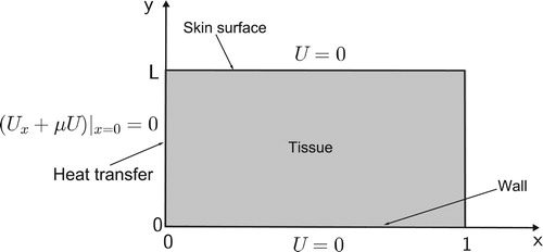
To demonstrate numerically the effectiveness of the forward solver developed in Section 3 we use a benchmark problem for the case $\mu =0$, with source function $f(x,y,t)$ chosen so that the unique solution to (1(1) $U_t=U_{xx}+U_{yy}-p\left(t\right)U(x,y,t)+f(x,y,t),(x,y,t)\in ]0,1[\times ]0,L[\times ]0,\mathcal{T}],$(1) )–(5(5) $U(x,y,0)=\phi (x,y),(x,y)\in [0,1]\times [0,L].$(5) ) is (45) $U(x,y,t)=\sin \left(\pi y\right)e^{-{\pi }^{2}t}{\sin }^3\left(\pi x\right),0\le x,y\le 1,0\le t\le 0.5$(45) with perfusion coefficient defined by $p\left(t\right)=e^{{\pi }^{2}t},0\le t\le 0.5$. It is not difficult to show that for this test problem the energy function is given by (46) $E\left(t\right)=\frac{8}{3{\pi }^2}{e}^{-{\pi }^{2}t}.$(46) Calculation of the forward problem is made using $21\times 21$ Chebyshev grid points and the auxiliary initial value problem (25(25) $\begin{array}{rl}{W}^{\prime }\left(t\right)& =G(t,W),t>0,\\ W\left(0\right)& =U_0,\end{array}$(25) ) is solved by using Crank–Nicolson method with timestep $h=0.5/200=0.0025$ (i.e.with N = 200). Exact solution $U(x,y,t)$, numerical solution $W(x,y,t)$ and the corresponding error at t = 0.5, $|U(x,y,0.5)-W(x,y,0,5)|$, all are displayed in Figure 2. This test problem is also considered in [11] (see Example 4.1) and solved by using finite differences with stepsize $h\approx 8\times {10}^{-6}$. The accuracy obtained in this way is approximately of the order ${10}^{-4}$. This contrasts significantly with our results obtained with much fewer grid points and with pointwise error of the order ${10}^{-8}$.

Figure 2. Exact solution and numerical solution of model (1(1) $U_t=U_{xx}+U_{yy}-p\left(t\right)U(x,y,t)+f(x,y,t),(x,y,t)\in ]0,1[\times ]0,L[\times ]0,\mathcal{T}],$(1) )and corresponding error.

Next, to assess the approximation error of Clenshaw–Curtis quadrature rule we use the approximate solution W to calculate energy values according to (44(44) ${\hat{E}}_{\ell }\left(\alpha \right)\approx w^T{\mathsf{U}}_{\ell }\left(\alpha \right)w,$(44) ) with n + 1 = 21 Chebyshev points. Outcome of the calculations, as well as the corresponding pointwise error, are displayed in Figure 3. Note that the approximation error in energy values is approximately ${10}^{-6}$.

Figure 3. Left: Energy values and their Chebyshev-Clenshaw–Curtis based approximations. Right: Pointwise error.

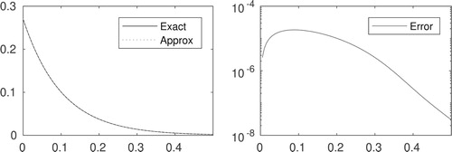
To further evaluate the approximation error of Clenshaw–Curtis quadrature rule, energy values were calculated using Gaussian quadrature with the same number of points. Results displayed in Figure 4 show what is often observed in practice: both quadrature rules have essentially the same accuracy, see again [43].

Figure 4. Comparison of quadrature rules efficiency. The error for Clenshaw–Curtis and Gaussian quadrature rules are labelled by Error CC and Error Gauss, respectively.

6.2. Reconstruction examples

In our examples, the forward solver is implemented as described in the previous subsection and the Levenberg method looks for a parametrized coefficient $p\left(t\right)$ based on a linear spline basis [44] associated with m + 1 = 21 equally distributed points. Thus the Jacobian matrix ${\mathsf{J}}^k$ at iteration k is of order $200\times 21$ and highly sparse due to the local properties of the spline basis being used. Noisy measurements are simulated by adding Gaussian random noise to the exact data $E_{\ell }=E\left(t_{\ell }\right)$, $t_{\ell }=\ell h$, such that ${\tilde{E}}_{\ell }=E_{\ell }+{ϵ}_{\ell },\ell =1,\dots ,200,$where ${ϵ}_{\ell }$ are zero-mean random numbers scaled in such a way that relative noise level in data is specified as $\parallel \tilde{\mathsf{E}}-\mathsf{E}\parallel =\mathrm{N}\mathrm{L}\parallel \mathsf{E}\parallel .$Constant $\mathrm{N}\mathrm{L}$ stands for relative noise level whereas $\mathsf{E}$ and $\tilde{\mathsf{E}}$ denote vectors containing noise-free and noisy measurements. To stop the iterative process, we use the discrepancy principle, i.e. the iterations stop at the first k such that $\parallel \hat{\mathsf{E}}\left({\alpha }_{\delta }^k\right)-\tilde{\mathsf{E}}\parallel \le \tau \delta ,\tau ⪆1.$In all computations, the error norm was used as input data and the discrepancy principle was implemented with $\tau =\mathrm{1.01.}$ We consider two numerical examples to illustrate the effectiveness of the estimation method.

6.2.1. Example 1

This example, taken from [11], considers the case $\mu =0$ and has a solution given by the pair $\left\{p\right(t),U(x,y,t\left)\right\}=\{e^{{\pi }^{2}t},\sin (\pi y)e^{-{\pi }^{2}t}{\sin }^3(\pi x\left)\right\}.$The source term and energy are, respectively, $\begin{array}{rl}f(x,y,t)& =-\sin \left(\pi y\right)e^{-{\pi }^{2}t}\sin \left(\pi x\right)[9{\pi }^2{\cos }^2(\pi x)-3{\pi }^2-e^{{\pi }^{2}t}{\cos }^2(\pi x\left)\right],\\ E\left(t\right)& =\frac{8}{3{\pi }^2}{e}^{-{\pi }^{2}t}.\end{array}$To evaluate the robustness of the estimation method to noise, we consider data as described above with three noise levels, namely $\mathrm{N}\mathrm{L}=1\mathrm{\%},0.5\mathrm{\%},0.1\mathrm{\%},$ and for each noise level we calculate the relative error in the reconstruction defined as $\mathrm{R}\mathrm{E}=\parallel p_{\mathrm{e}\mathrm{x}}-p_{\mathrm{e}\mathrm{s}\mathrm{t}\mathrm{i}\mathrm{m}}\parallel /\parallel p_{\mathrm{e}\mathrm{x}}\parallel ,$where $p_{\mathrm{e}\mathrm{x}}$ and $p_{\mathrm{e}\mathrm{s}\mathrm{t}\mathrm{i}\mathrm{m}}$ denote the vectors containing pointwise values of exact and estimated $p\left(t\right)$, respectively. Exact data and noisy data with noise level $1\mathrm{\%}$ as well as the results of the numerical inversion for all tested noise levels are displayed in Figure 5. Relative errors are displayed in Table 1. Note that the pointwise estimation error improves as the noise level decreases and few iterations were required for the stopping criterion to be satisfied, e.g. for NL=$1\mathrm{\%}$ the criterion was satisfied after k = 9 iterations.

Figure 5. Left: Exact and noisy data for numerical inversion. Noisy data in this illustration corresponds to noise level $1\mathrm{\%}$. Right: Exact coefficient $p\left(t\right)$ and recovered ones.

Table 1. Relative error in reconstructing $p\left(t\right)$.

NL	1%	0.5%	0.01%
RE	0.2535	0.1318	0.0344

To further evaluate the effectiveness of the proposed inversion method, the recovered perfusion coefficient, the source function and initial data in model (1(1) $U_t=U_{xx}+U_{yy}-p\left(t\right)U(x,y,t)+f(x,y,t),(x,y,t)\in ]0,1[\times ]0,L[\times ]0,\mathcal{T}],$(1) ) – (5(5) $U(x,y,0)=\phi (x,y),(x,y)\in [0,1]\times [0,L].$(5) ) were used as input data to predict temperature values through our forward solver. The predicted computed values, denoted here by $\hat{U}(x,y,t)$, and pointwise errors $|U(x,y,t)-\hat{U}(x,y,t)|$ for the case $\mathrm{N}\mathrm{L}=1\mathrm{\%}$ at the time level t = 0.5 are displayed in Figure 6. Notice that the error in the recovered $\hat{U}$ for this case is about ${10}^{-4}$.

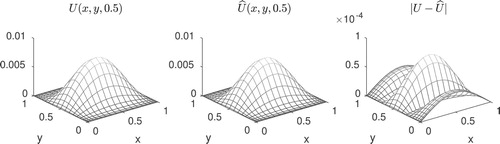
Figure 6. Exact and recovered temperatures and corresponding pointwise error.

6.2.2. Example 2

We now address the reconstruction problem using a test problem with $\mu =-1$. In this case, the solution to the inverse problem is $\left\{p\right(t),U(x,y,t\left)\right\}=\left\{\frac{e^t}{(2+\sin (3\pi t\left)\right)},(1+x-x^2)\sin \left(\pi y\right)(2+\sin (3\pi t\left)\right)e^{-t}\right\}.$In addition, the source term, the initial condition and the energy function are, respectively, $\begin{array}{rl}f(x,y,t)& =-\frac{e^{-t}\phi (x,y)}{2}(-\sin (3\pi t)+3\pi \cos (3\pi t)-2)\\ & +2\sin \left(\pi y\right)(2+\sin (3\pi t\left)\right)e^{-t}+{\pi }^2\frac{\phi (x,y)}{2}(2+\sin (3\pi t\left)\right)e^{-t}+\frac{\phi (x,y)}{2},\\ \phi (x,y)& =2(1+x-x^2)\sin \left(\pi y\right),\\ E\left(t\right)& =\frac{7}{3\pi }(2+\sin (3\pi t\left)\right)e^{-t}.\end{array}$For this example the forward solver also uses $21\times 21$ grid points but the time step is h = 0.05 and the semidiscrete model (25(25) $\begin{array}{rl}{W}^{\prime }\left(t\right)& =G(t,W),t>0,\\ W\left(0\right)& =U_0,\end{array}$(25) ) is solved on $[0,1].$ As in Example 1, to evaluate the reconstruction method we also consider noise data with three noise levels, $\mathrm{N}\mathrm{L}=1\mathrm{\%},0.5\mathrm{\%},0.1\mathrm{\%}.$ Numerical results displayed in Figure 7 together with relative errors presented in Table 2 show that the quality of the reconstruction improves as the noise level decreases and indicate therefore that the method is robust. As for the number of iterations spent by the whole process, in this example, for $\mathrm{N}\mathrm{L}=1\mathrm{\%}$ the stopping index was k = 5.

Figure 7. Left: Exact and noisy data for numerical inversion. Noisy data in this illustration corresponds to noise level $1\mathrm{\%}$. Right: Exact coefficient $p\left(t\right)$ and recovered ones.

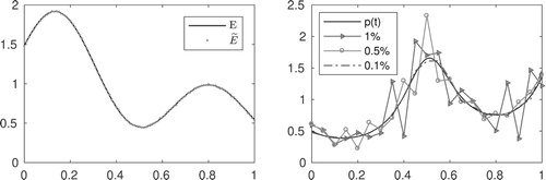
Table 2. Relative error in reconstructing $p\left(t\right)$.

NL	1%	0.5%	0.01%
RE	0.3130	0.041	0.0364

Finally, as in Example 2, we also use the recovered coefficient $p\left(t\right)$ in order to calculate predicted temperature values $\hat{U}(x,y,t)$. These values and the corresponding pointwise error for $\mathrm{N}\mathrm{L}=1\mathrm{\%}$ are displayed in Figure 8.

Figure 8. Exact and recovered temperatures and corresponding pointwise error.

6.2.3. Example 3: Hard test

We consider a test problem using data that can be accepted as experimental and that allow us to objectively challenge the effectiveness of the proposed method. The data set we have in mind consists of energy values corresponding to a bioheat transfer problem (1(1) $U_t=U_{xx}+U_{yy}-p\left(t\right)U(x,y,t)+f(x,y,t),(x,y,t)\in ]0,1[\times ]0,L[\times ]0,\mathcal{T}],$(1) )-(5(5) $U(x,y,0)=\phi (x,y),(x,y)\in [0,1]\times [0,L].$(5) ), with $\mu =-1$, initial condition (47) $U_0(x,y,0)\doteq \phi (x,y)=e^{x(x-1{)}^2}y(1-y),$(47) and source function (48) $f(x,y,t)=e^{-\pi t}\sin \left(\pi x\right)\sin \left(\pi y\right).$(48) For the moment, the perfusion coefficient p is an arbitrary function in $C[0,\mathcal{T}]$ and therefore, no solution to the bioheat transfer problem is available. In this example we use $\mathcal{T}=1$.

For ease of exposition, we will start with an analysis of the input data $(\phi ,f)$ described above to ensure that the inverse problem of interest has a unique solution. Next, we will describe how the data set is generated and, finally, we will describe results of the reconstruction.

6.2.4. Analysis

We will show that the data set we have in mind arises from a well-posed problem by checking that the input data $(\phi ,f)$ and the associated energy E meet the conditions $\left(A_1\right)$ –$\left(A_3\right)$ in Theorem 2.1. In fact, it is easy to check that φ satisfies the boundary conditions in $\left(A_1\right)$ and that (49) ${\phi }_{0,2n-1}=\sqrt{2}\left({\int }_0^1{e}^{x(x-1{)}^2}(1-x)\mathrm{d}x\right)\left({\int }_0^{1}y(1-y)\sin \left(\right(2n-1\left)\pi y\right)\mathrm{d}y\right).$(49) Clearly, the first integral in (49(49) ${\phi }_{0,2n-1}=\sqrt{2}\left({\int }_0^1{e}^{x(x-1{)}^2}(1-x)\mathrm{d}x\right)\left({\int }_0^{1}y(1-y)\sin \left(\right(2n-1\left)\pi y\right)\mathrm{d}y\right).$(49) ) is positive. As for the second, integration by parts shows that ${\int }_0^{1}y(1-y)\sin \left(\right(2n-1\left)\pi y\right)\mathrm{d}y=\frac{4}{\left[\right(2n-1)\pi {]}^3}>0,$so that ${\phi }_{0,2n-1}>0$. We can argue analogously to show that (50) $\begin{array}{r}{\phi }_{2m,2n-1}=\sqrt{2}\left({\int }_0^1{e}^{x(x-1{)}^2}\sin \left(2\pi mx\right)\mathrm{d}x\right)\left({\int }_0^{1}y(1-y)\sin \left(\right(2n-1\left)\pi y\right)\mathrm{d}y\right)>0.\end{array}$(50) Therefore, since φ is sufficiently regular, all conditions in $\left(A_1\right)$ are satisfied. In turn, due to the definition of function f in (48(48) $f(x,y,t)=e^{-\pi t}\sin \left(\pi x\right)\sin \left(\pi y\right).$(48) ), it follows that the boundary conditions in $\left(A_2\right)$ are satisfied and that $f_{2m,2n-1}\left(t\right)=0$ holds true. Thus, since f is sufficiently regular, all conditions in $\left(A_2\right)$ holds true.

Now since both $\left(A_1\right)$ and $\left(A_2\right)$ are satisfied, for given $p\in C[0,\mathcal{T}]$, p>0, we are allowed to conclude that the forward problem (1(1) $U_t=U_{xx}+U_{yy}-p\left(t\right)U(x,y,t)+f(x,y,t),(x,y,t)\in ]0,1[\times ]0,L[\times ]0,\mathcal{T}],$(1) )–(5(5) $U(x,y,0)=\phi (x,y),(x,y)\in [0,1]\times [0,L].$(5) ) has a unique solution $U\in C^{2,1}\left(\overline{{\mathrm{\Omega }}_{\mathcal{T}}}\right)$, which, as already mentioned, is expressed in series form in terms of the basis $\left\{Z_{m,n}\right\}$ [11]. Therefore, to check that $\left(A_3\right)$ holds true it is sufficient to show that the associated energy E defined in (6(6) ${\int }_0^1{\int }_0^{1}U(x,y,t)\mathrm{d}x\mathrm{d}y=E\left(t\right),0\le t\le \mathcal{T},$(6) ) satisfies $E\left(t\right)>0,t\in [0,\mathcal{T}]$. For this we will show that $U\ge 0$ on $\overline{{\mathrm{\Omega }}_{\mathcal{T}}}$. Indeed, assume the contrary and set $m_0=\underset{(x,y,t)\in \overline{{\mathrm{\Omega }}_{\mathcal{T}}}}{min}U(x,y,t)<0$. As $\phi \ge 0$ on $\overline{\mathrm{\Omega }}$, it is clear that U does not attain $m_0$ in $\overline{\mathrm{\Omega }}\times \left\{0\right\}$. From the maximum principle for parabolic equations [45, Theorem 1.5, p. 53], if U attains $m_0$ at some point in ${\mathrm{\Omega }}_{\mathcal{T}}$ then $U=m_0$ throughout ${\mathrm{\Omega }}_{\mathcal{T}}$; clearly, this contradicts (1(1) $U_t=U_{xx}+U_{yy}-p\left(t\right)U(x,y,t)+f(x,y,t),(x,y,t)\in ]0,1[\times ]0,L[\times ]0,\mathcal{T}],$(1) ), as both p and f given by (48(48) $f(x,y,t)=e^{-\pi t}\sin \left(\pi x\right)\sin \left(\pi y\right).$(48) ) are positive on ${\mathrm{\Omega }}_{\mathcal{T}}$. As a consequence, taking into account (2(2) $\begin{array}{rl}& U(0,y,t)=U(1,y,t),0\le y\le L,0\le t\le \mathcal{T},\end{array}$(2) )–(4(4) $\begin{array}{rl}& U(x,0,t)=U(x,L,t)=0,0\le x\le 1,0\le t\le \mathcal{T},\end{array}$(4) ), U attains $m_0$ at a point $(0,y,t)$, 0<y<1 or at a point $(1,y,t)$, 0<y<1, $0<t\le \mathcal{T}$. Assuming that U attains $m_0$ at a point $(0,y,t)$, 0<y<1, using again the maximum principle, it follows that $U_x(0,y,t)>0$, i.e.$U_x(0,y,t)+\mu U(0,y,t)>0$, which contradicts (3(3) $\begin{array}{rl}& U_x(0,y,t)+\mu U(0,y,t)=0,0\le y\le L,0\le t\le \mathcal{T},\end{array}$(3) ). From condition (2(2) $\begin{array}{rl}& U(0,y,t)=U(1,y,t),0\le y\le L,0\le t\le \mathcal{T},\end{array}$(2) ), assuming that U attains $m_0$ at a point $(1,y,t)$, 0<y<1, U attains $m_0$ also at $(0,y,t)$, so we have the same contradiction. Thus, we conclude that $U\ge 0$ on $\overline{{\mathrm{\Omega }}_{\mathcal{T}}}$ and from (6(6) ${\int }_0^1{\int }_0^{1}U(x,y,t)\mathrm{d}x\mathrm{d}y=E\left(t\right),0\le t\le \mathcal{T},$(6) ) that $E\left(t\right)\ge 0$. Now, for each $0\le t\le \mathcal{T}$ fixed, as f is not identically null and taking into account that $U(x,y,t)$ satisfies (1(1) $U_t=U_{xx}+U_{yy}-p\left(t\right)U(x,y,t)+f(x,y,t),(x,y,t)\in ]0,1[\times ]0,L[\times ]0,\mathcal{T}],$(1) ), it is clear that $U(x,y,t)$ is not identically null on $\mathrm{\Omega }\times \left\{t\right\}$. Then, from the continuity of U in $\overline{{\mathrm{\Omega }}_{\mathcal{T}}}$, we conclude that $E\left(t\right)>0$ for all $0\le t\le \mathcal{T}$.

In our numerical experiments we will use (51) $p\left(t\right)=e^{\sin \left(2\pi t\right)}.$(51)

6.2.5. Generating data

Roughly speaking, to simulate experimental energy data for the bioheat transfer problem of interest we will rely on temperature data obtained from the numerical solution of a nearby problem. For this, we first use the Crank–Nicolson method to calculate approximate solutions $W_k$ to the forward problem (1(1) $U_t=U_{xx}+U_{yy}-p\left(t\right)U(x,y,t)+f(x,y,t),(x,y,t)\in ]0,1[\times ]0,L[\times ]0,\mathcal{T}],$(1) )–(5(5) $U(x,y,0)=\phi (x,y),(x,y)\in [0,1]\times [0,L].$(5) ), as described in (28(28) $\left[I-\frac{h}{2}(A-p_{k+1}I)\right]W_{k+1}=\left[I+\frac{h}{2}(A-p_{k}I)\right]W_k+\frac{h}{2}\left[S_k+S_{k+1}\right],k=0,\dots ,$(28) ), assuming that neither the initial condition $U(x,y,0)$ given in (47(47) $U_0(x,y,0)\doteq \phi (x,y)=e^{x(x-1{)}^2}y(1-y),$(47) ) nor the coefficient $p\left(t\right)$ in (51(51) $p\left(t\right)=e^{\sin \left(2\pi t\right)}.$(51) ) are exactly known. The source term, on the other hand, is assumed known and given in (48(48) $f(x,y,t)=e^{-\pi t}\sin \left(\pi x\right)\sin \left(\pi y\right).$(48) ). Then, to calculate discrete energy values $E_k$ we simply integrate the approximate solution at $t=t_k$ on $[0,1]\times [0,1]$ using the composite trapezoidal quadrature rule. However, we observe that, since the CPS method works on a grid based on Chebyshev points, to calculate energy values in this way the approximate solutions at each time step have to be interpolated on a regular grid. In our numerical calculations, to interpolate the data we use the built-in Matlab function interp2. In practice, the temperature data used in our calculations come from solving the forward problem with initial condition $\tilde{U}(x_i,y_j,0)=\phi (x_i,y_j)+{ϵ}_{i,j}$ and perturbed coefficient $\tilde{p}\left(t_k\right)=p\left(t_k\right)+{ϵ}_k$, where ${ϵ}_{i,j}$ and ${ϵ}_k$ denote random numbers with specified intensities. For the reconstruction problem, we will always use temperature data on a spatial grid of $21\times 21$ Chebyshev points at time steps of size h = 0.05. As an example of input data that we use to generate energy values, exact and perturbed initial condition, φ, $\tilde{U}$, as well as exact and perturbed coefficient, p, $\tilde{p}$, with a noise level of $3\mathrm{\%}$ in both cases, are displayed in Figure 9.

Figure 9. Exact and perturbed initial temperatures and exact and perturbed perfusion coefficient.

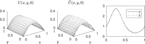
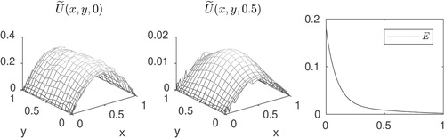
On the other hand, the initial condition ${\tilde{U}}_0$, the approximate numerical solution obtained by Crank–Nicolson method at t = 0.5, as well as the calculated energy values, are all displayed in Figure 10. It is worth emphasizing here that, since the Crank-Nicolson method is unconditionally stable, provided input errors are small, the approximate solutions $\tilde{U}(x_i,y_j,t_k)$ will not depart so much from $U(x_i,y_j,t_k)$. This justifies why we regard the actual temperature data as experimental.

Figure 10. Initial condition, predicted temperature at t = 0.5 and calculated energy.

6.2.6. Reconstruction results

We report numerical results obtained with the proposed method from data $E_k$, generated as described above, assuming that both $\tilde{U}$, $\tilde{p}$ (the input data) are affected by perturbations with the same intensity. We consider input data with three noise levels, ${\mathrm{N}\mathrm{L}}_{\mathrm{I}\mathrm{D}}=1\mathrm{\%},3\mathrm{\%},5\mathrm{\%}$. Before proceeding we observe that, since the purpose of the present example is to challenge the proposed method, in addition to addressing the reconstruction problem with the calculated energy values $E_k$ as input data, we also consider extra uncertainty in $E_k$ coming from additive random disturbances in $E_k$; the numerical experiment with this type of data is conducted considering two noise levels: ${\mathrm{N}\mathrm{L}}_{\mathrm{E}}=0.01\mathrm{\%},0.1\mathrm{\%}$. Further, for comparison purposes, in addition to the results obtained with the use of the spline basis, we also report results obtained with the method under the assumption that the perfusion coefficient is parameterized as a linear combination of Legendre polynomials on [0,1] of degree less than or equal to m (a subset of the Legendre basis of $L^2(0,1)$). That is, we also look for $p_m\approx p$ with $p_m\in {\tilde{\mathcal{P}}}_m=\mathrm{s}\mathrm{p}\mathrm{a}\mathrm{n}\{{\tilde{P}}_0,\dots ,{\tilde{P}}_m\}$, (52) $p_m\left(t\right)=\sum _{k=0}^m{\alpha }_k{\tilde{P}}_k\left(t\right),$(52) where ${\tilde{P}}_k$ denotes the shifted Legendre polynomial (53) ${\tilde{P}}_k\left(t\right)=P_k(2t-1),t\in [0,1],k=0,1,\dots ,$(53) being $P_k$ the classical Legendre polynomial of degree k. In our numerical calculations both bases (spline and polynomial) have dimension 21. Taking into account that we consider disturbances in the input data with three noise levels (${\mathrm{N}\mathrm{L}}_{\mathrm{I}\mathrm{D}}=1\mathrm{\%},3\mathrm{\%},5\mathrm{\%}$) and disturbances in the calculated energy also with three noise levels (${\mathrm{N}\mathrm{L}}_{\mathrm{E}}=0\mathrm{\%},0.01\mathrm{\%},0.1\mathrm{\%}$), the numerical results of the experiment can be organized into 9 cases, each of them associated to a pair $({\mathrm{N}\mathrm{L}}_{\mathrm{I}\mathrm{D}},{\mathrm{N}\mathrm{L}}_{\mathrm{E}})$. In Figure 11, we present results of four cases, which we consider as the most representative ones and that correspond to the combinations (S, S), (S, L), (L, S) and (L, L), where S and L stand for smallest and largest noise levels respectively.

Figure 11. Exact coefficient $p\left(t\right)$ and recovered ones.

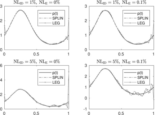
As we can see, except for the case (S,S), i.e.($1\mathrm{\%},0\mathrm{\%}$), the quality of the reconstructions obtained with the Legendre basis look significantly inferior when compared to that obtained with the spline basis. To assess the results in a more efficient way, we calculate relative errors in the reconstructions for both approaches. Results are shown in Table 3 not only confirm what we visually concluded from Figure 11, but also that, for this test problem, the reconstruction quality obtained with the spline basis is superior.

Table 3. Relative error in estimated coefficients.

Case	(S,S)	(S,L)	(L,S)	(L,L)
SPLIN	0.019971	0.025204	0.048042	0.063594
LEG	0.067864	0.067181	0.217524	0.124550

To close this comparison, we mention that we also performed other experiments using the Legendre basis with dimensions 11 (m = 10) and 16 (m = 15). The quality of the results followed the same trend as those presented above and, therefore, are not reported here.

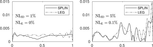
In the last part of the numerical experiment, we first solve the semidiscrete problem with noise-free input data and consider the numerical solution at $t_k=hk,k=1,\dots ,200$ as exact temperature data. Then, with $U_0(x,y,0)$ and the estimated coefficient $p_m\left(t\right)$ as input data, we solve the semidiscrete problem to predict temperature values at the same time steps and compare them with the exact ones through relative errors in the Frobenius norm. The results of such a comparison for the cases (S, S) and (L, L) are shown in Figure 12. From this figure, it can be seen that the errors in the predicted temperatures do not exceed $0.5\mathrm{\%}$ and $1.5\mathrm{\%}$ for the cases (S,S) and (L,L), respectively, which is quite notable since in these cases the largest error in $p_m$ is about $12\mathrm{\%}$. We believe that the reason of this is the ill-posed nature of the problem: very different input parameters can lead to very similar results.

Figure 12. Relative errors in predicted temperatures with recovered coefficient as input data.

7. Concluding remarks

The paper considers the determination of a time-dependent lowest order coefficient of a 2D parabolic equation with Ionkin nonlocal boundary condition and total energy measurement. Existence and uniqueness and global well-posedness of the problem are studied by using a series expansion method based on eigenfunctions of a nonself-adjoint spatial differential operator. The system of eigenfunctions is proved to be a basis with parenthesis of the solution space. For numerically solving the problem, the sought coefficient was determined by a nonlinear least-squares method combined with the CPS collocation method to solve the forward problem. Numerical results showed that the method is able to provide accurate and stable numerical reconstructions.

As future work, we plan to study an inverse problem associated with a 2D parabolic equation described as (54) $U_t=\mathrm{\Delta }U-p\left(t\right)U(x,y,t)+f(x,y,t),\mathrm{\Delta }U=U_{xx}+U_{yy},(x,y,t)\in {\mathrm{\Omega }}_{\mathcal{T}},$(54) with nonclassical boundary conditions (55) $\begin{array}{rl}& {\mu }_0{U}_x(0,y,t)={\mu }_{1}U(0,y,t),0\le y\le 1,0\le t\le \mathcal{T},\end{array}$(55) (56) $\begin{array}{rl}& \mathrm{\Delta }U(1,y,t)+{\mu }_2{U}_x(1,y,t)+{\mu }_{3}U(1,y,t)=0,0\le y\le 1,0\le t\le \mathcal{T},\end{array}$(56) (57) $\begin{array}{rl}& U(x,0,t)=U(x,1,t)=0,0\le x\le 1,0\le t\le \mathcal{T},\end{array}$(57) and initial condition (58) $U(x,y,0)=\phi (x,y),(x,y)\in \overline{\mathrm{\Omega }}.$(58) The above mathematical model is intended to describe the bioheat transfer process of a rectangular perfused tissue with thickness and width equal to 1, upper skin at y = 1, a wall between the tissue and an adjoint blood vessel at y = 0 under adiabatic condition at x = 0 and the Wentzell boundary condition at x = 1, which is describing a situation like the Robin boundary condition, with the additional feature that the boundary has the capacity of storing heat.

The inverse problem that we plan to study consists of finding a pair $\{p,U\}\in C[0,\mathcal{T}]\times C^{2,1}\left(\overline{{\mathrm{\Omega }}_{\mathcal{T}}}\right)$ satisfying (54(54) $U_t=\mathrm{\Delta }U-p\left(t\right)U(x,y,t)+f(x,y,t),\mathrm{\Delta }U=U_{xx}+U_{yy},(x,y,t)\in {\mathrm{\Omega }}_{\mathcal{T}},$(54) ) – (58(58) $U(x,y,0)=\phi (x,y),(x,y)\in \overline{\mathrm{\Omega }}.$(58) ) and the total integral overdetermination condition (59) ${\int }_0^1{\int }_0^{1}U(x,y,t)\mathrm{d}x\mathrm{d}y=E\left(t\right).$(59) The mathematical analysis of the problem (54(54) $U_t=\mathrm{\Delta }U-p\left(t\right)U(x,y,t)+f(x,y,t),\mathrm{\Delta }U=U_{xx}+U_{yy},(x,y,t)\in {\mathrm{\Omega }}_{\mathcal{T}},$(54) )–(59(59) ${\int }_0^1{\int }_0^{1}U(x,y,t)\mathrm{d}x\mathrm{d}y=E\left(t\right).$(59) ) requires solving the 2D spectral problem $\begin{array}{rl}& \frac{{\mathrm{\partial }}^{2}Z}{\mathrm{\partial }{x}^2}+\frac{{\mathrm{\partial }}^{2}Z}{\mathrm{\partial }{y}^2}+\sigma Z=0,0<x,y<1,\\ & {\mu }_2\frac{\mathrm{\partial }Z}{\mathrm{\partial }x}(1,y)=\left(\sigma -{\mu }_3\right)Z(1,y),{\mu }_0\frac{\mathrm{\partial }Z}{\mathrm{\partial }x}(0,y)={\mu }_{1}Z(0,y),0\le y\le 1,\\ & Z(x,0)=Z(x,1)=0,0\le x\le 1,\end{array}$where σ is the separation parameter. This kind of 2D spectral problems is new and there is not enough literature available [39,46]. Theoretical and numerical analysis of (54(54) $U_t=\mathrm{\Delta }U-p\left(t\right)U(x,y,t)+f(x,y,t),\mathrm{\Delta }U=U_{xx}+U_{yy},(x,y,t)\in {\mathrm{\Omega }}_{\mathcal{T}},$(54) )–(59(59) ${\int }_0^1{\int }_0^{1}U(x,y,t)\mathrm{d}x\mathrm{d}y=E\left(t\right).$(59) ) are the subject of ongoing research.

Disclosure statement

No potential conflict of interest was reported by the author(s).

Additional information

Funding

F.S.V.B. work was supported by CNPq, Brazil.

References

- Bedin L, Bazán FSV. On the 2D bioheat equation with convective boundary conditions and its numerical realization via a highly accurate approach. Appl Math Comp. 2014;236:422–436.
- Fan J, Wang L. Analytical theory of bioheat transport. J Appl Phys. 2011;109:104702.
- Pennes HH. Analysis of tissue and arterial blood temperatures in the resting human forearm. J Appl Physiol. 1948;1:93–122.
- Lakhssassi A, Kengne E, Semmaoui H. Modified Pennes' equation modelling bioheat transfer in living tissues: analytical and numerical analysis. Nat Sci. 2010;2:1375–1385.
- Cao L, Qin QH, Zhao N. An RBMFS model for analysing thermal behavior of skin tissues. Int J Heat Mass Transfer. 2010;53:1298–1307.
- Azizbavov EI. The nonlocal inverse problem of the identification of the lowest coefficient and the right-hand side in a second-order parabolic equation with integral conditions. Bound Value Probl. 2019;2019:1–19.
- Ionkin NI. Solution of a boundary-value problem in heat conduction with a non-classical boundary condition. Differ Equ. 1977;13:294–304.
- Hazanee A, Lesnic D. Determination of a time-dependent coefficient in the bioheat equation. Int J Mech Sci. 2014;88:259–266.
- Hochmuth R. Homogenization for a non-local coupling model. Appl Anal. 2008;87:1311–1323.
- Ionkin NI, Morozova VA. The two-dimensional heat equation with nonlocal boundary conditions. Differ Equ. 2000;36:982–987.
- Ismailov MI, Erkovana S. Inverse problem of finding the coefficient of the lowest term in two-dimensional heat equation with Ionkin-type boundary condition. Comput Math Math Phys. 2019;59:791–808.
- Ciesielski M, Duda M, Mochnacki B. Comparison of bioheat transfer numerical models based on the Pennes and Cattaneo–Vernotte equations. J Appl Math Comput Mech. 2016;15:33–38.
- Grysa K, Maciag A. Trefftz method in solving the Pennes' and single-phase-lag heat conduction problems with perfusion in the skin. Int J Numer Methods Heat Fluid Flow. 2019;30:3231–3246.
- Grysa K, Maciag A. Identifying heat source intensity in treatment of cancerous tumor using therapy based on local hyperthermia – The Trefftz method approachs. J Therm Biol. 2019;84:16–25.
- Iljaz J, Skerget L. Blood perfusion estimation in heterogeneous tissue using BEM based algorithm. Eng Anal Bound Elem. 2014;39:75–87.
- Majchrzak E, Turchan L. The general boundary element method for 3D dual-phase lag model of bioheat transfer. Eng Anal Bound Elem. 2015;50:76–82.
- Ismailov MI, Bazán FSV, Bedin L. Time-dependent perfusion coefficient estimation in a bioheat transfer problem. Comput Phys Commun. 2018;230:50–58.
- Grabski JK, Lesnic D, Johansson BT. Identification of a time-dependent bioheat blood perfusion coefficient. Int Commun Heat Mass Transfer. 2016;75:18–22.
- Lesnic D, Ivanchov MI. Determination of the time-dependent perfusion coefficient in the bioheat equation. Appl Math Lett. 2015;39:96–100.
- Lin Y. An inverse problem for a class of quasi-linear parabolic equations. SIAM J Math Anal. 1991;22:146–156.
- Prilepko AI, Solov'ev VV. On the solvability of inverse boundary value problems for the determination of the coefficient preceding the lower derivative in a parabolic equation. Differ Equ. 1987;23:136–143.
- Yousefi SA. Finding a control parameter in a one-dimensional parabolic inverse problem by using the Bernstein Galerkin method. Inverse Probl Sci Eng. 2009;17:821–828.
- Ismailov MI, Kanca F. An inverse coefficient problem for a parabolic equation in the case of nonlocal boundary and overdetermination conditions. Math Methods Appl Sci. 2011;34:692–702.
- Ivanchov MI, Pabyrivska NV. Simultaneous determination of two coefficients of a parabolic equation in the case of nonlocal and integral conditions. Ukr Math J. 2001;53:674–684.
- Kerimov NB, Ismailov MI. Direct and inverse problems for the heat equation with a dynamic-type boundary condition. IMA J Appl Math. 2015;80:1519–1533.
- Kerimov NB, Ismailov MI. An inverse coefficient problem for the heat equation in the case of nonlocal boundary conditions. J Math Anal Appl. 2012;396:546–554.
- Cannon JR, Lin Y, Wang S. Determination of source parameter in parabolic equation. Meccanica. 1992;27:85–94.
- Daoud DS, Subasi D. A splitting up algorithm for the determination of the control parameter in multi-dimensional parabolic problem. Appl Math Comput. 2005;166:584–595.
- Dehghan M. Numerical methods for two-dimensional parabolic inverse problem with energy overspecification cation. Int J Comput Math. 2000;77:441–455.
- Pyatkov SG. Solvability of some inverse problems for parabolic equations. J Inv Ill-Posed Probl. 2004;12:397–412.
- Bedin L, Bazán FSV. A note on existence and uniqueness of solutions for a 2D bioheat problem. Appl Anal. 2017;96:590–605.
- Bazán FSV, Bedin L, Borges LS. Space-dependent perfusion coefficient estimation in a 2D bioheat transfer problem. Comput Phys Commun. 2017;214:18–30.
- Fornberg B. A practical guide to pseudospectral methods. Cambridge: Cambridge University Press; 1996.
- Trefethen LN. Spectral methods in matlab. Philadelphia (PA): SIAM; 2000.
- Levenberg K.A. Method for the solution of certain non-linear problems in least squares. Quart Appl Math. 1944;2:164–168.
- Marquardt DW. An algorithm for least squares estimation of nonlinear parameters. J Soc Ind Appl Math. 1963;11:431–441.
- Naimark MA. Linear differential operators: elementary theory of linear differential operators. New York (NY): Frederick Ungar Publishing Co.; 1967.
- Lo CY. Boundary value problems. Singapore: World Scientfic; 2000.
- Yu. Kapustin N, Moiseev EI. A spectral problem for the Laplace operator in the square with a spectral parameter in the boundary condition. Differ Equ. 1998;34:663–668.
- Beck JV, Arnold KJ. Parameter estimation in engineering and science. New York (NY): Wiley; 1977.
- Dennis J, Schnabel R. Numerical methods for unconstrained optimization and nonlinear equations. Englewood Cliffs (NJ): Prentice Hall; 1983.
- Yamashita N, Fukushima M. On the rate of convergence of the Levenberg–Marquardt method. Comput (Suppl). 2001;15:239–249.
- Trefethen LN. Is gauss quadrature better than Clenshaw–Curtis? SIAM Rev. 2008;50:67–87.
- Golub HH, Ortega JM. Scientific computing and differential equations-an introduction to numerical methods. San Diego (CA): Academic Press; 1992.
- Pao CV. Nonlinear parabolic and elliptic equations. New York (NY): Plenum Press; 1992.
- Yu. Kapustin N. Basis properties of a problem for the Laplace operator on the square with spectral parameter in a boundary condition. Differ Equ. 2017;53:563–565.