A modified quasi-boundary value method for a backward problem for the inhomogeneous time conformable fractional heat equation in a cylinder

ABSTRACT

The time conformable heat equation is a generalization of classical heat equation involved local and limit-based derivative, which is called conformable fractional derivative. In this paper, we study a backward problem for the time conformable fractional heat equation defined in cylindrical coordinates for the axis-symmetric case which is a severely ill-posed problem. By using a modified quasi-boundary value method, the problem is regularized and some new error estimates are obtained. The numerical experiment shows that the method is feasible and effective.

Keywords:

• Backward heat problem
• quasi-boundary value method
• conformable derivative
• error estimate

AMS Subject Classifications:

• 35R25
• 35R30
• 65J20
• 65M30

1. Introduction

Fractional calculus appears in many fields of science and engineering, such as signal processing, finance and plasma physics, aerodynamics and control systems, viscoelasticity, bioengineering and biomedical [1–3]. Many researchers tried to give a definition of fractional derivative. Most of them used an integral form of fractional derivative. One of the well-known fractional derivatives is the Riemann–Liouville fractional order derivative, for $\alpha \in [n-1,n)$, the $\ast \ast$ derivative of f is ${}_{RL}{D}_a^{\alpha }\left(f\right)\left(t\right)=\frac{1}{\mathrm{\Gamma }(n-\alpha )}\frac{{\mathrm{d}}^n}{\mathrm{d}{t}^n}{\int }_a^t\frac{f\left(x\right)}{(t-x{)}^{\alpha -n+1}}\mathrm{d}x.$ The second one is the so-called Caputo derivative, for $\alpha \in [n-1,n)$, the $\ast \ast$ derivative of f is ${}_C{D}_a^{\alpha }\left(f\right)\left(t\right)=\frac{1}{\mathrm{\Gamma }(n-\alpha )}{\int }_a^t\frac{f^{\left(n\right)}\left(x\right)}{(t-x{)}^{\alpha -n+1}}\mathrm{d}x.$ Obviously, the RL and Caputo fractional derivatives are non-local operators represented by convolutional integrals with weakly singular kernels. The inverse problem for the heat equation where the time-derivative is in the sense of Caputo fractional order is of great interest to many researchers as these operators are effective for modelling of sub/super-anomalous behaviours of physical processes [4–12].

Although non-local fractional derivatives give natural memory and genetic effects in the physical system, the fractional derivatives obtained in this kind of calculus seem very complicated and lose some basic properties of general derivatives, such as product rule and chain rule. Accordingly, the authors in [13] define a new well-behaved simple fractional derivative called ‘the conformable derivative’ depending just on the basic limit defnition of the derivative and this concept seems to satisfy all the requirements of the standard derivative. Namely,

Definition 1.1

[13] (CFD)

Given a function $f:[0,\mathrm{\infty })\to \mathbb{R}$. Then the conformable fractional derivative of order $\alpha \in (0,1)$ of f is defined by $D_t^{\alpha }f\left(t\right)=\underset{h\to 0}{lim}\frac{f(t+h{t}^{1-\alpha })-f\left(t\right)}{h},$ for all t>0.

If f is $\alpha -differentiable$ in some $(0,a)$ and $\underset{t\to 0^{+}}{lim}{D}_t^{\alpha }f\left(t\right)$ exists, then define $D_t^{\alpha }f\left(0\right)=\underset{t\to 0^{+}}{lim}{D}_t^{\alpha }f\left(t\right).$ Note that if f is differentiable, then $D_t^{\alpha }f\left(t\right)=t^{1-\alpha }{f}^{\mathrm{\prime }}\left(t\right),$ where $f^{\mathrm{\prime }}\left(t\right)=\underset{h\to 0}{lim}\frac{f(t+h)-f\left(t\right)}{h}$. They then proved the product rule, the fractional mean value theorem solved some (conformable) fractional differential equations where the fractional exponential function ${\mathrm{e}}^{\frac{t^{\alpha }}{\alpha }}$ played an important rule. While in case of well-known fractional calculus Mittag-Leffler functions generalized exponential functions.

This new theory is studied by Abdeljawad [14] and Atangana [15]. In addition, Anderson and Ulness in [16] gave a potential application of the conformable derivative in quantum mechanics. In [17], Dazhi Zhao et al. generalized the definition of conformable fractional derivative of order $\alpha \in (0,1)$ by means of Linear Extended Gteaux derivative (LEGD) to general conformable fractional derivative (GCFD). They also gave physical and geometrical interpretations of this new derivative which thus indicate potential applications in physics and engineering. The definition of the GCFD of arbitrary order given by them is as follows:

Definition 1.2

[17] (GCFD of arbitrary order)

Let $\alpha \in (n,n+1]$, for some $n\in \mathbb{N}$ and f be n-differentiable at t>0. Then the α-fractional derivative of f is defined as $\begin{array}{rl}{D}_{\psi }^{\alpha }f\left(t\right)& =D_{\psi }^{\alpha -n}{D}^{n}f\left(t\right)\\ & =\underset{ϵ\to 0}{lim}\frac{f^{\left(n\right)}(t+ϵ\psi (t,\alpha -n\left)\right)-f^{\left(n\right)}\left(t\right)}{ϵ},\end{array}$ if the limit exists. When $\psi (t,\alpha )=t^{1-\alpha }$, $D_{\psi }^{\alpha }f\left(t\right)$ coincides with Khalil's definition [13]. In other words, CFD is a special case of GCFD. Then geometrical interpretations of the GCFD is that the gradient of a function f projects onto a function $\psi (t,\alpha -n)$ or a special function $\psi (t,\alpha -n)$ projects onto the gradient of a function f from a different viewpoint. And physical interpretation of GCFD can be regarded as a special velocity, its direction and strength rely on $\psi (t,\alpha -n)$. Although the conformable derivative has no nonlocality [18,19], there exists some advantages for this kind of derivative such as the formula of integral by parts.

On partial differential equations with the conformable derivative, there are several studies. Çenesiz, Kurt and Nane in [20] gave stochastic solutions of conformable fractional Cauchy problems by running the processes corresponding to Cauchy problems with a nonlinear deterministic clock. In [21], Çenesiz et al. studied the solutions of time and space fractional heat differential equations and Fourier sine and Fourier cosine transform definitions were given. Hammad and Khalil in [22] applied conformable Fourier series to interpret the solution for the conformable heat equation. In [23], Avci et al. aimed to find the fundamental solution of a conformable heat equation acting on a radial symmetric plate. In [24], Yavuz et al. aimed the numerical inverse Laplace homotopy technique for solving some interesting 1-D time-fractional heat equations based on the Laplace homotopy perturbation method. In [25], Vu et al. studied an inverse time problem for the nonhomogeneous heat equation under the conformable derivative and obtained a Hölder-type estimation error for the whole time interval. In [26], the authors introduced the conformable double Laplace transform which could be used to solve fractional partial differential equations that represented many physical and engineering models. In [27], R. I. Nuruddeen et al. considered the fractional heat diffusion models featuring fractional order derivatives in both the Caputo's and the new conformable derivatives to further investigate the development by analysing two solutions. For more literature on solutions, refer to [28–33].

Based on the above research, the inverse problem of heat equation under conformal derivatives is naturally considered. But there are few mathematical results about the time conformable heat equation in an axis-symmetric cylinder. In this study, we are concerned with a backward problem for the inhomogeneous time conformable fractional heat equation in a cylinder. Let us consider the following time conformable heat equation in an axis-symmetric cylinder (1) $\frac{{\mathrm{\partial }}^{\alpha }}{\mathrm{\partial }{t}^{\alpha }}u(r,z,t)=a\left(\frac{{\mathrm{\partial }}^{2}u}{\mathrm{\partial }{r}^2}+\frac{1}{r}\frac{\mathrm{\partial }u}{\mathrm{\partial }r}+\frac{{\mathrm{\partial }}^{2}u}{\mathrm{\partial }{z}^2}\right)+f(r,z,t),$(1) subjected to the following initial and boundary conditions given respectively as (2) $u(r,z,0)=h(r,z),0<r\le R,$(2) and (3) $\begin{array}{rl}& u(R,z,t)=u(0,z,t)=0,t>0,0<z\le L,\\ & u(r,0,t)=u(r,L,t)=0,t>0,0<r\le R,\\ & u\text{is finite},t>0,0<r\le R,0<z\le L,\end{array}$(3) where $\frac{{\mathrm{\partial }}^{\alpha }}{\mathrm{\partial }{t}^{\alpha }}$ represents the conformable fractional derivative of order $\alpha (0<\alpha \le 1)$. a is thermal diffusivity constant and $f(r,z,t)$ denotes a heat source.

Solving this equation with the given information $f(r,z,t)$ and $h(r,z)$ is called the direct problem. From the information given at final time (4) $u(r,z,T)=g(r,z),$(4) the goal of the inverse problem is to recover the information $\left\{u\right(r,z,t),h(r,z\left)\mathrm{i}\mathrm{n}\mathrm{i}\mathrm{t}\mathrm{i}\mathrm{a}\mathrm{l}\text{condition}\right\}$ for $0\le t<T$. This inverse backward problem is an ill-posed problem. We propose a modified quasi-boundary value method to solve it (refer to [34]). In our method, the convergence speed will gradually increase corresponding to different levels of smoothness of the exact solution. Under some suitable conditions for exact solution u, we will introduce an error estimate of order ${\delta }^{\frac{\alpha p}{T^{\alpha }+\alpha p}}(p>0)$.

The remainder of this paper is organized as follows. In Section 2, formulation for the problem (1(1) $\frac{{\mathrm{\partial }}^{\alpha }}{\mathrm{\partial }{t}^{\alpha }}u(r,z,t)=a\left(\frac{{\mathrm{\partial }}^{2}u}{\mathrm{\partial }{r}^2}+\frac{1}{r}\frac{\mathrm{\partial }u}{\mathrm{\partial }r}+\frac{{\mathrm{\partial }}^{2}u}{\mathrm{\partial }{z}^2}\right)+f(r,z,t),$(1) )–(4(4) $u(r,z,T)=g(r,z),$(4) ) and the ill-posedness of the backward heat problem are presented. We construct the regularized solution by a modified quasi-boundary value method and study the well-posedness of problem (22(22) $\begin{array}{lll}& \frac{{\mathrm{\partial }}^{\alpha }}{\mathrm{\partial }{t}^{\alpha }}w(r,z,t)=a\left(\frac{{\mathrm{\partial }}^{2}w}{\mathrm{\partial }{r}^2}+\frac{1}{r}\frac{\mathrm{\partial }w}{\mathrm{\partial }r}+\frac{{\mathrm{\partial }}^{2}w}{\mathrm{\partial }{z}^2}\right)+f^{\nu }(r,z,t),& (r,z,t)\in \mathrm{\Omega }\times (0,T),\\ & w(0,z,t)=w(R,z,t)=w(r,0,t)=w(r,L,t)=0,& (r,z,t)\in \mathrm{\Omega }\times [0,T],\\ & w(r,z,T)=g^{\nu }(r,z),& (r,z)\in \mathrm{\Omega },\end{array}$(22) )–(24(24) $\begin{array}{rl}{g}^{\nu }(r,z)& =\sum _{m,n=1}^{\mathrm{\infty }}\frac{g_{mn}}{1+\nu {\mathrm{e}}^{ab{\lambda }_{mn}\frac{T^{\alpha }}{\alpha }}}{J}_0\left(\frac{{\mu }_{n}r}{R}\right)\sin \left(\frac{m\pi }{L}z\right).\end{array}$(24) ) in Section 3. Section 4 provides the detailed convergence analysis under different levels of the smoothness of the exact solution. Finally, in Section 5, we give some numerical examples to verify the theory.

2. Formulation for the problem and the ill-posed backward heat problem

We introduce the Lebesgue space associated with the measure rdr, i.e. $L_r^2\left(\mathrm{\Omega }\right)=\left\{v:\mathrm{\Omega }\to \mathbb{R}\mathrm{m}\mathrm{e}\mathrm{a}\mathrm{s}\mathrm{u}\mathrm{r}\mathrm{a}\mathrm{b}\mathrm{l}\mathrm{e};{\int }_{\mathrm{\Omega }}{v}^2(r,z)r\mathrm{d}r\mathrm{d}z<+\mathrm{\infty }\right\},$ which is a Hilbert space with the scalar product $〈u,v{〉}_r={\int }_{\mathrm{\Omega }}u(r,z)v(r,z)r\mathrm{d}r\mathrm{d}z,$ and the corresponding norm is given by ${∥v∥}_{L_r^2\left(\mathrm{\Omega }\right)}={\left({\int }_{\mathrm{\Omega }}{v}^2(r,z)r\mathrm{d}r\mathrm{d}z\right)}^{\frac{1}{2}}.$ The weighted Sobolev spaces defined on Ω are introduced as follows $H_r^m\left(\mathrm{\Omega }\right)=\left\{v\in L_r^2\left(\mathrm{\Omega }\right);\frac{{\mathrm{\partial }}^{p+q}v}{\mathrm{\partial }{r}^p\mathrm{\partial }{z}^q}\in L_r^2\left(\mathrm{\Omega }\right),p,q\in \mathbb{N},p+q\le m\right\}.$ Throughout this paper, for the convenience of writing, we denote $〈\cdot ,\cdot {〉}_r$ and $\parallel \cdot \parallel$ by the inner product and the norm in $L_r^2\left(\mathrm{\Omega }\right)$, where $\mathrm{\Omega }=(0,R)\times (0,L)$. Let's first consider what the weak solution of the problem (1(1) $\frac{{\mathrm{\partial }}^{\alpha }}{\mathrm{\partial }{t}^{\alpha }}u(r,z,t)=a\left(\frac{{\mathrm{\partial }}^{2}u}{\mathrm{\partial }{r}^2}+\frac{1}{r}\frac{\mathrm{\partial }u}{\mathrm{\partial }r}+\frac{{\mathrm{\partial }}^{2}u}{\mathrm{\partial }{z}^2}\right)+f(r,z,t),$(1) )–(3(3) $\begin{array}{rl}& u(R,z,t)=u(0,z,t)=0,t>0,0<z\le L,\\ & u(r,0,t)=u(r,L,t)=0,t>0,0<r\le R,\\ & u\text{is finite},t>0,0<r\le R,0<z\le L,\end{array}$(3) ) is. We call a function $u\in L^2\left(\right[0,T];H_{r,0}^1(\mathrm{\Omega }\left)\right)\bigcap C^1\left(\right(0,T);H_r^2(\mathrm{\Omega }\left)\right)$ to be a weak solution for problem (1(1) $\frac{{\mathrm{\partial }}^{\alpha }}{\mathrm{\partial }{t}^{\alpha }}u(r,z,t)=a\left(\frac{{\mathrm{\partial }}^{2}u}{\mathrm{\partial }{r}^2}+\frac{1}{r}\frac{\mathrm{\partial }u}{\mathrm{\partial }r}+\frac{{\mathrm{\partial }}^{2}u}{\mathrm{\partial }{z}^2}\right)+f(r,z,t),$(1) )–(3(3) $\begin{array}{rl}& u(R,z,t)=u(0,z,t)=0,t>0,0<z\le L,\\ & u(r,0,t)=u(r,L,t)=0,t>0,0<r\le R,\\ & u\text{is finite},t>0,0<r\le R,0<z\le L,\end{array}$(3) ) if (5) $\frac{{\mathrm{d}}^{\alpha }}{\mathrm{d}{t}^{\alpha }}{〈u(\cdot ,\cdot ,t),W〉}_{L_r^2\left(\mathrm{\Omega }\right)}-{〈u(\cdot ,\cdot ,t),\mathrm{△}W〉}_{L_r^2\left(\mathrm{\Omega }\right)}={〈f(\cdot ,\cdot ,t),W〉}_{L_r^2\left(\mathrm{\Omega }\right)},$(5) for all functions $W\in H_{r,0}^1\left(\mathrm{\Omega }\right)\bigcap H_r^2\left(\mathrm{\Omega }\right)$. Here, $\mathrm{△}W=a(\frac{{\mathrm{\partial }}^{2}W}{\mathrm{\partial }{r}^2}+\frac{1}{r}\frac{\mathrm{\partial }W}{\mathrm{\partial }r}+\frac{{\mathrm{\partial }}^{2}W}{\mathrm{\partial }{z}^2})$. In fact, it is enough to choose W in the orthogonal basis of $L_r^2\left(\mathrm{\Omega }\right)$. So, next, we derive an analytical solution for the problem (1(1) $\frac{{\mathrm{\partial }}^{\alpha }}{\mathrm{\partial }{t}^{\alpha }}u(r,z,t)=a\left(\frac{{\mathrm{\partial }}^{2}u}{\mathrm{\partial }{r}^2}+\frac{1}{r}\frac{\mathrm{\partial }u}{\mathrm{\partial }r}+\frac{{\mathrm{\partial }}^{2}u}{\mathrm{\partial }{z}^2}\right)+f(r,z,t),$(1) )–(3(3) $\begin{array}{rl}& u(R,z,t)=u(0,z,t)=0,t>0,0<z\le L,\\ & u(r,0,t)=u(r,L,t)=0,t>0,0<r\le R,\\ & u\text{is finite},t>0,0<r\le R,0<z\le L,\end{array}$(3) ) based on the eigenfunction expansion and the eigenfunction system are complete and orthogonal with weight r in $L_r^2\left(\mathrm{\Omega }\right)$.

Let $u(r,z,t)=X\left(r\right)Y\left(z\right)T\left(t\right)$, substitute it into the corresponding homogeneous equation for (1.1), then we get $\frac{\frac{{\mathrm{d}}^{2}X}{\mathrm{d}{r}^2}+\frac{1}{r}\frac{\mathrm{d}X}{\mathrm{d}r}}{X\left(r\right)}+\frac{\frac{{\mathrm{d}}^{2}Y}{\mathrm{d}{z}^2}}{Y\left(z\right)}-\frac{1}{a}\frac{\frac{{\mathrm{d}}^{\alpha }T}{\mathrm{d}{t}^{\alpha }}}{T\left(t\right)}=0.$ This equation is true, meaning that the items in the formula should be constants, so we get $\frac{\frac{{\mathrm{d}}^{2}X}{\mathrm{d}{r}^2}+\frac{1}{r}\frac{\mathrm{d}X}{\mathrm{d}r}}{X\left(r\right)}=-\rho ,\frac{\frac{d^{2}Y}{\mathrm{d}{z}^2}}{Y\left(z\right)}=-l,\frac{1}{a}\frac{\frac{{\mathrm{d}}^{\alpha }T}{\mathrm{d}{t}^{\alpha }}}{T\left(t\right)}=-\lambda ,$ where $\rho ,l,\lambda$ are the undetermined constants introduced when separating variables, $\rho +l=\lambda$. Further, by separating the boundary conditions (3(3) $\begin{array}{rl}& u(R,z,t)=u(0,z,t)=0,t>0,0<z\le L,\\ & u(r,0,t)=u(r,L,t)=0,t>0,0<r\le R,\\ & u\text{is finite},t>0,0<r\le R,0<z\le L,\end{array}$(3) ), we get the following results (6) $\begin{array}{rl}& \frac{{\mathrm{d}}^{2}X}{\mathrm{d}{r}^2}+\frac{1}{r}\frac{\mathrm{d}X}{\mathrm{d}r}+\rho X=0,r\in (0,R),\\ & X\left(0\right)=X\left(R\right)=0.\end{array}$(6) (7) $\begin{array}{rl}& \frac{{\mathrm{d}}^{2}Y}{\mathrm{d}{z}^2}+lY=0,z\in (0,L),\\ & Y\left(0\right)=Y\left(L\right)=0.\end{array}$(7)

The eigenvalues of problem (6(6) $\begin{array}{rl}& \frac{{\mathrm{d}}^{2}X}{\mathrm{d}{r}^2}+\frac{1}{r}\frac{\mathrm{d}X}{\mathrm{d}r}+\rho X=0,r\in (0,R),\\ & X\left(0\right)=X\left(R\right)=0.\end{array}$(6) ) are (8) ${\rho }_n={\left(\frac{{\mu }_n}{R}\right)}^2,n=1,2,\dots ,$(8) and the corresponding eigenfunctions are $X_n\left(r\right)=J_0\left(\frac{{\mu }_{n}r}{R}\right),n=1,2,\dots ,$ where ${\mu }_n$ denotes the zeros of Bessel function $J_0$.

The eigenvalues of problem (7(7) $\begin{array}{rl}& \frac{{\mathrm{d}}^{2}Y}{\mathrm{d}{z}^2}+lY=0,z\in (0,L),\\ & Y\left(0\right)=Y\left(L\right)=0.\end{array}$(7) ) are (9) $l_m={\left(\frac{m\pi }{L}\right)}^2,m=1,2,\dots ,$(9) and the corresponding eigenfunctions are $Y_m\left(z\right)=\sin \left(\frac{m\pi }{L}z\right),m=1,2,\dots .$ $\left\{J_0\right(\frac{{\mu }_{n}r}{R})\sin (\frac{m\pi }{L}z){\}}_{n,m\ge 1}$ are complete and orthogonal in $L_r^2\left(\mathrm{\Omega }\right)$ and the follow orthogonality properties $\begin{array}{rl}& {\int }_0^R{J}_0\left(\frac{{\mu }_{n}r}{R}\right)J_0\left(\frac{{\mu }_{i}r}{R}\right)r\mathrm{d}r=\left\{\begin{array}{ll}0,& n\ne i,\\ \frac{R^2{J}_1^2\left({\mu }_n\right)}{2},& n=i,\end{array}\right.\\ & {\int }_0^L\sin \left(\frac{m\pi }{L}z\right)\sin \left(\frac{k\pi }{L}z\right)\mathrm{d}z=\left\{\begin{array}{ll}0,& m\ne k,\\ \frac{L}{2},& m=k.\end{array}\right.\end{array}$ Thus the solution $u(r,z,t)$ and nonhomogeneous term $f(r,z,t)$ of problem (1(1) $\frac{{\mathrm{\partial }}^{\alpha }}{\mathrm{\partial }{t}^{\alpha }}u(r,z,t)=a\left(\frac{{\mathrm{\partial }}^{2}u}{\mathrm{\partial }{r}^2}+\frac{1}{r}\frac{\mathrm{\partial }u}{\mathrm{\partial }r}+\frac{{\mathrm{\partial }}^{2}u}{\mathrm{\partial }{z}^2}\right)+f(r,z,t),$(1) )–(3(3) $\begin{array}{rl}& u(R,z,t)=u(0,z,t)=0,t>0,0<z\le L,\\ & u(r,0,t)=u(r,L,t)=0,t>0,0<r\le R,\\ & u\text{is finite},t>0,0<r\le R,0<z\le L,\end{array}$(3) ) can be represented as follows (10) $\begin{array}{rl}u(r,z,t)& =\sum _{m,n=1}^{\mathrm{\infty }}{u}_{mn}\left(t\right)J_0\left(\frac{{\mu }_{n}r}{R}\right)\sin \left(\frac{m\pi }{L}z\right),\end{array}$(10) (11) $\begin{array}{rl}f(r,z,t)& =\sum _{m,n=1}^{\mathrm{\infty }}{f}_{mn}\left(t\right)J_0\left(\frac{{\mu }_{n}r}{R}\right)\sin \left(\frac{m\pi }{L}z\right),\end{array}$(11) where $u_{mn}\left(t\right)$, $f_{mn}\left(t\right)$ are the generalized Fourier coefficients.

By substituting (10(10) $\begin{array}{rl}u(r,z,t)& =\sum _{m,n=1}^{\mathrm{\infty }}{u}_{mn}\left(t\right)J_0\left(\frac{{\mu }_{n}r}{R}\right)\sin \left(\frac{m\pi }{L}z\right),\end{array}$(10) ), (11(11) $\begin{array}{rl}f(r,z,t)& =\sum _{m,n=1}^{\mathrm{\infty }}{f}_{mn}\left(t\right)J_0\left(\frac{{\mu }_{n}r}{R}\right)\sin \left(\frac{m\pi }{L}z\right),\end{array}$(11) ) into (1(1) $\frac{{\mathrm{\partial }}^{\alpha }}{\mathrm{\partial }{t}^{\alpha }}u(r,z,t)=a\left(\frac{{\mathrm{\partial }}^{2}u}{\mathrm{\partial }{r}^2}+\frac{1}{r}\frac{\mathrm{\partial }u}{\mathrm{\partial }r}+\frac{{\mathrm{\partial }}^{2}u}{\mathrm{\partial }{z}^2}\right)+f(r,z,t),$(1) ) and (2(2) $u(r,z,0)=h(r,z),0<r\le R,$(2) ), in this case, the conformable fractional differential equation reduces to (12) $\begin{array}{rl}& \frac{{\mathrm{d}}^{\alpha }{u}_{mn}\left(t\right)}{\mathrm{d}{t}^{\alpha }}+a\left[{\left(\frac{{\mu }_n}{R}\right)}^2+{\left(\frac{m\pi }{L}\right)}^2\right]u_{mn}\left(t\right)=f_{mn}\left(t\right),\end{array}$(12) (13) $\begin{array}{rl}& u_{mn}\left(0\right)=h_{mn},\end{array}$(13) where (14) $\begin{array}{rl}{f}_{mn}\left(t\right)& =\frac{4}{L{R}^2{J}_1^2\left({\mu }_n\right)}{\int }_0^R{\int }_0^L{J}_0\left(\frac{{\mu }_{n}r}{R}\right)\sin \left(\frac{m\pi }{L}z\right)f(r,z,t)r\mathrm{d}r\mathrm{d}z,\end{array}$(14) (15) $\begin{array}{rl}{h}_{mn}& =\frac{4}{L{R}^2{J}_1^2\left({\mu }_n\right)}{\int }_0^R{\int }_0^L{J}_0\left(\frac{{\mu }_{n}r}{R}\right)\sin \left(\frac{m\pi }{L}z\right)h(r,z)r\mathrm{d}r\mathrm{d}z.\end{array}$(15) By applying fractional Laplace transform (detailed solution process can be found in [35]), we can get the solution of the initial problem (12(12) $\begin{array}{rl}& \frac{{\mathrm{d}}^{\alpha }{u}_{mn}\left(t\right)}{\mathrm{d}{t}^{\alpha }}+a\left[{\left(\frac{{\mu }_n}{R}\right)}^2+{\left(\frac{m\pi }{L}\right)}^2\right]u_{mn}\left(t\right)=f_{mn}\left(t\right),\end{array}$(12) )–(13(13) $\begin{array}{rl}& u_{mn}\left(0\right)=h_{mn},\end{array}$(13) ) as follows (16) $u_{mn}\left(t\right)=h_{mn}{\mathrm{e}}^{-a\left[{\left(\frac{{\mu }_n}{R}\right)}^2+{\left(\frac{m\pi }{L}\right)}^2\right]\frac{t^{\alpha }}{\alpha }}+{\int }_0^t{\mathrm{e}}^{-a\left[{\left(\frac{{\mu }_n}{R}\right)}^2+{\left(\frac{m\pi }{L}\right)}^2\right]\frac{t^{\alpha }-s^{\alpha }}{\alpha }}{s}^{\alpha -1}{f}_{mn}\left(s\right)\mathrm{d}s.$(16) Denote by ${\lambda }_{mn}={\left(\frac{{\mu }_n}{R}\right)}^2+{\left(\frac{m\pi }{L}\right)}^2,$ by substituting (16(16) $u_{mn}\left(t\right)=h_{mn}{\mathrm{e}}^{-a\left[{\left(\frac{{\mu }_n}{R}\right)}^2+{\left(\frac{m\pi }{L}\right)}^2\right]\frac{t^{\alpha }}{\alpha }}+{\int }_0^t{\mathrm{e}}^{-a\left[{\left(\frac{{\mu }_n}{R}\right)}^2+{\left(\frac{m\pi }{L}\right)}^2\right]\frac{t^{\alpha }-s^{\alpha }}{\alpha }}{s}^{\alpha -1}{f}_{mn}\left(s\right)\mathrm{d}s.$(16) ) into (10(10) $\begin{array}{rl}u(r,z,t)& =\sum _{m,n=1}^{\mathrm{\infty }}{u}_{mn}\left(t\right)J_0\left(\frac{{\mu }_{n}r}{R}\right)\sin \left(\frac{m\pi }{L}z\right),\end{array}$(10) ), we get (17) $u(r,z,t)=\sum _{m,n=1}^{\mathrm{\infty }}\left(h_{mn}{\mathrm{e}}^{-a{\lambda }_{mn}\frac{t^{\alpha }}{\alpha }}+{\int }_0^t{\mathrm{e}}^{-a{\lambda }_{mn}\frac{t^{\alpha }-s^{\alpha }}{\alpha }}{s}^{\alpha -1}{f}_{mn}\left(s\right)\mathrm{d}s\right)J_0\left(\frac{{\mu }_{n}r}{R}\right)\sin \left(\frac{m\pi }{L}z\right).$(17) Applying (4(4) $u(r,z,T)=g(r,z),$(4) ) and (17(17) $u(r,z,t)=\sum _{m,n=1}^{\mathrm{\infty }}\left(h_{mn}{\mathrm{e}}^{-a{\lambda }_{mn}\frac{t^{\alpha }}{\alpha }}+{\int }_0^t{\mathrm{e}}^{-a{\lambda }_{mn}\frac{t^{\alpha }-s^{\alpha }}{\alpha }}{s}^{\alpha -1}{f}_{mn}\left(s\right)\mathrm{d}s\right)J_0\left(\frac{{\mu }_{n}r}{R}\right)\sin \left(\frac{m\pi }{L}z\right).$(17) ), we obtain (18) $g_{mn}=h_{mn}{\mathrm{e}}^{-a{\lambda }_{mn}\frac{T^{\alpha }}{\alpha }}+{\int }_0^T{\mathrm{e}}^{-a{\lambda }_{mn}\frac{T^{\alpha }-s^{\alpha }}{\alpha }}{s}^{\alpha -1}{f}_{mn}\left(s\right)\mathrm{d}s,$(18) where $g_{mn}=\frac{4}{L{R}^2{J}_1^2\left({\mu }_n\right)}{\int }_0^R{\int }_0^L{J}_0\left(\frac{{\mu }_{n}r}{R}\right)\sin \left(\frac{m\pi }{L}z\right)g(r,z)r\mathrm{d}r\mathrm{d}z.$ Using (18(18) $g_{mn}=h_{mn}{\mathrm{e}}^{-a{\lambda }_{mn}\frac{T^{\alpha }}{\alpha }}+{\int }_0^T{\mathrm{e}}^{-a{\lambda }_{mn}\frac{T^{\alpha }-s^{\alpha }}{\alpha }}{s}^{\alpha -1}{f}_{mn}\left(s\right)\mathrm{d}s,$(18) ), (17(17) $u(r,z,t)=\sum _{m,n=1}^{\mathrm{\infty }}\left(h_{mn}{\mathrm{e}}^{-a{\lambda }_{mn}\frac{t^{\alpha }}{\alpha }}+{\int }_0^t{\mathrm{e}}^{-a{\lambda }_{mn}\frac{t^{\alpha }-s^{\alpha }}{\alpha }}{s}^{\alpha -1}{f}_{mn}\left(s\right)\mathrm{d}s\right)J_0\left(\frac{{\mu }_{n}r}{R}\right)\sin \left(\frac{m\pi }{L}z\right).$(17) ) becomes (19) $\begin{array}{rl}u(r,z,t)& =\sum _{m,n=1}^{\mathrm{\infty }}\left({\mathrm{e}}^{a{\lambda }_{mn}\frac{T^{\alpha }-t^{\alpha }}{\alpha }}{g}_{mn}-{\int }_t^T{\mathrm{e}}^{-a{\lambda }_{mn}\frac{t^{\alpha }-s^{\alpha }}{\alpha }}{s}^{\alpha -1}{f}_{mn}\left(s\right)\mathrm{d}s\right)J_0\left(\frac{{\mu }_{n}r}{R}\right)\sin \left(\frac{m\pi }{L}z\right)\\ & =\sum _{m,n=1}^{\mathrm{\infty }}{\mathrm{e}}^{a{\lambda }_{mn}\frac{T^{\alpha }-t^{\alpha }}{\alpha }}\left(g_{mn}-{\int }_t^T{\mathrm{e}}^{a{\lambda }_{mn}\frac{s^{\alpha }-T^{\alpha }}{\alpha }}{s}^{\alpha -1}{f}_{mn}\left(s\right)\mathrm{d}s\right)J_0\left(\frac{{\mu }_{n}r}{R}\right)\sin \left(\frac{m\pi }{L}z\right).\end{array}$(19) If we denote ${\omega }_n\left(r\right)=\frac{\sqrt{2}}{R{J}_1\left({\mu }_n\right)}{J}_0\left(\frac{{\mu }_{n}r}{R}\right)$, ${\phi }_m\left(z\right)=\sqrt{\frac{2}{L}}\sin \left(\frac{m\pi }{L}z\right)$ and ${\psi }_{m,n}(r,z)={\omega }_n\left(r\right){\phi }_m\left(z\right)$, then it is easy to check that the eigenfunctions $\left\{{\psi }_{m,n}\right(r,z){\}}_{n,m\ge 1}$ form an orthonormal basis in $L_r^2\left(\mathrm{\Omega }\right)$. Using the eigenfunctions as the basises, we can expand (20) $u(r,z,t)=\sum _{m,n=1}^{\mathrm{\infty }}{〈u(r,z,t),{\psi }_{m,n}(r,z)〉}_r{\psi }_{m,n}(r,z).$(20) Let $g^{\delta }$ be the measured data satisfying (21) $\parallel g^{\delta }-g\parallel \le \delta .$(21) Since t<T, from (19(19) $\begin{array}{rl}u(r,z,t)& =\sum _{m,n=1}^{\mathrm{\infty }}\left({\mathrm{e}}^{a{\lambda }_{mn}\frac{T^{\alpha }-t^{\alpha }}{\alpha }}{g}_{mn}-{\int }_t^T{\mathrm{e}}^{-a{\lambda }_{mn}\frac{t^{\alpha }-s^{\alpha }}{\alpha }}{s}^{\alpha -1}{f}_{mn}\left(s\right)\mathrm{d}s\right)J_0\left(\frac{{\mu }_{n}r}{R}\right)\sin \left(\frac{m\pi }{L}z\right)\\ & =\sum _{m,n=1}^{\mathrm{\infty }}{\mathrm{e}}^{a{\lambda }_{mn}\frac{T^{\alpha }-t^{\alpha }}{\alpha }}\left(g_{mn}-{\int }_t^T{\mathrm{e}}^{a{\lambda }_{mn}\frac{s^{\alpha }-T^{\alpha }}{\alpha }}{s}^{\alpha -1}{f}_{mn}\left(s\right)\mathrm{d}s\right)J_0\left(\frac{{\mu }_{n}r}{R}\right)\sin \left(\frac{m\pi }{L}z\right).\end{array}$(19) ) we know that, when ${\lambda }_{mn}$ become larger, ${\mathrm{e}}^{a{\lambda }_{mn}\frac{T^{\alpha }-t^{\alpha }}{\alpha }}$ increases very quickly. Therefore, the term ${\mathrm{e}}^{a{\lambda }_{mn}\frac{T^{\alpha }-t^{\alpha }}{\alpha }}$ is the cause of instability and the problem (1(1) $\frac{{\mathrm{\partial }}^{\alpha }}{\mathrm{\partial }{t}^{\alpha }}u(r,z,t)=a\left(\frac{{\mathrm{\partial }}^{2}u}{\mathrm{\partial }{r}^2}+\frac{1}{r}\frac{\mathrm{\partial }u}{\mathrm{\partial }r}+\frac{{\mathrm{\partial }}^{2}u}{\mathrm{\partial }{z}^2}\right)+f(r,z,t),$(1) )–(4(4) $u(r,z,T)=g(r,z),$(4) ) is ill-posed and a regularization is necessary. In the next Section, we shall construct the regularized solution and establish the approximation for the problem.

Remark 2.1

When $\alpha =1$, (17(17) $u(r,z,t)=\sum _{m,n=1}^{\mathrm{\infty }}\left(h_{mn}{\mathrm{e}}^{-a{\lambda }_{mn}\frac{t^{\alpha }}{\alpha }}+{\int }_0^t{\mathrm{e}}^{-a{\lambda }_{mn}\frac{t^{\alpha }-s^{\alpha }}{\alpha }}{s}^{\alpha -1}{f}_{mn}\left(s\right)\mathrm{d}s\right)J_0\left(\frac{{\mu }_{n}r}{R}\right)\sin \left(\frac{m\pi }{L}z\right).$(17) ) is the solution of the classical first-order time-derivative initial value problem of partial differential equation with inhomogeneous term. When $\alpha \to 0$, ${\mathrm{e}}^{a{\lambda }_{mn}\frac{T^{\alpha }-t^{\alpha }}{\alpha }}\to (\frac{T}{t}{)}^{a{\lambda }_{mn}}$, the ill-posedness becomes weak. This is a very interesting phenomenon for inverse problems involved fractional derivative.

3. Well-posedness of the regularized problem

In this section, we will apply a modified quasi-boundary value method to regularize (1(1) $\frac{{\mathrm{\partial }}^{\alpha }}{\mathrm{\partial }{t}^{\alpha }}u(r,z,t)=a\left(\frac{{\mathrm{\partial }}^{2}u}{\mathrm{\partial }{r}^2}+\frac{1}{r}\frac{\mathrm{\partial }u}{\mathrm{\partial }r}+\frac{{\mathrm{\partial }}^{2}u}{\mathrm{\partial }{z}^2}\right)+f(r,z,t),$(1) )–(4(4) $u(r,z,T)=g(r,z),$(4) ). We will consider problem (1(1) $\frac{{\mathrm{\partial }}^{\alpha }}{\mathrm{\partial }{t}^{\alpha }}u(r,z,t)=a\left(\frac{{\mathrm{\partial }}^{2}u}{\mathrm{\partial }{r}^2}+\frac{1}{r}\frac{\mathrm{\partial }u}{\mathrm{\partial }r}+\frac{{\mathrm{\partial }}^{2}u}{\mathrm{\partial }{z}^2}\right)+f(r,z,t),$(1) )–(4(4) $u(r,z,T)=g(r,z),$(4) ) with adjusted information so that the adjusted problem can be well-posed and approximate to the original problem. Starting from the ideas mentioned in the paper of [34], we consider the following approximate problem (22) $\begin{array}{lll}& \frac{{\mathrm{\partial }}^{\alpha }}{\mathrm{\partial }{t}^{\alpha }}w(r,z,t)=a\left(\frac{{\mathrm{\partial }}^{2}w}{\mathrm{\partial }{r}^2}+\frac{1}{r}\frac{\mathrm{\partial }w}{\mathrm{\partial }r}+\frac{{\mathrm{\partial }}^{2}w}{\mathrm{\partial }{z}^2}\right)+f^{\nu }(r,z,t),& (r,z,t)\in \mathrm{\Omega }\times (0,T),\\ & w(0,z,t)=w(R,z,t)=w(r,0,t)=w(r,L,t)=0,& (r,z,t)\in \mathrm{\Omega }\times [0,T],\\ & w(r,z,T)=g^{\nu }(r,z),& (r,z)\in \mathrm{\Omega },\end{array}$(22) where (23) $\begin{array}{rl}{f}^{\nu }(r,z,t)& =\sum _{m,n=1}^{\mathrm{\infty }}\frac{f_{mn}\left(t\right)}{1+\nu {\mathrm{e}}^{ab{\lambda }_{mn}\frac{T^{\alpha }}{\alpha }}}{J}_0\left(\frac{{\mu }_{n}r}{R}\right)\sin \left(\frac{m\pi }{L}z\right),\end{array}$(23) (24) $\begin{array}{rl}{g}^{\nu }(r,z)& =\sum _{m,n=1}^{\mathrm{\infty }}\frac{g_{mn}}{1+\nu {\mathrm{e}}^{ab{\lambda }_{mn}\frac{T^{\alpha }}{\alpha }}}{J}_0\left(\frac{{\mu }_{n}r}{R}\right)\sin \left(\frac{m\pi }{L}z\right).\end{array}$(24) In formulas (22(22) $\begin{array}{lll}& \frac{{\mathrm{\partial }}^{\alpha }}{\mathrm{\partial }{t}^{\alpha }}w(r,z,t)=a\left(\frac{{\mathrm{\partial }}^{2}w}{\mathrm{\partial }{r}^2}+\frac{1}{r}\frac{\mathrm{\partial }w}{\mathrm{\partial }r}+\frac{{\mathrm{\partial }}^{2}w}{\mathrm{\partial }{z}^2}\right)+f^{\nu }(r,z,t),& (r,z,t)\in \mathrm{\Omega }\times (0,T),\\ & w(0,z,t)=w(R,z,t)=w(r,0,t)=w(r,L,t)=0,& (r,z,t)\in \mathrm{\Omega }\times [0,T],\\ & w(r,z,T)=g^{\nu }(r,z),& (r,z)\in \mathrm{\Omega },\end{array}$(22) )–(24(24) $\begin{array}{rl}{g}^{\nu }(r,z)& =\sum _{m,n=1}^{\mathrm{\infty }}\frac{g_{mn}}{1+\nu {\mathrm{e}}^{ab{\lambda }_{mn}\frac{T^{\alpha }}{\alpha }}}{J}_0\left(\frac{{\mu }_{n}r}{R}\right)\sin \left(\frac{m\pi }{L}z\right).\end{array}$(24) ), $f_{mn}\left(t\right)$, $g_{mn}$ are defined by (14(14) $\begin{array}{rl}{f}_{mn}\left(t\right)& =\frac{4}{L{R}^2{J}_1^2\left({\mu }_n\right)}{\int }_0^R{\int }_0^L{J}_0\left(\frac{{\mu }_{n}r}{R}\right)\sin \left(\frac{m\pi }{L}z\right)f(r,z,t)r\mathrm{d}r\mathrm{d}z,\end{array}$(14) ) and (15(15) $\begin{array}{rl}{h}_{mn}& =\frac{4}{L{R}^2{J}_1^2\left({\mu }_n\right)}{\int }_0^R{\int }_0^L{J}_0\left(\frac{{\mu }_{n}r}{R}\right)\sin \left(\frac{m\pi }{L}z\right)h(r,z)r\mathrm{d}r\mathrm{d}z.\end{array}$(15) ), ν is a regularization parameter depending on δ. The real number $b\ge 1$ is a constant.

From (17(17) $u(r,z,t)=\sum _{m,n=1}^{\mathrm{\infty }}\left(h_{mn}{\mathrm{e}}^{-a{\lambda }_{mn}\frac{t^{\alpha }}{\alpha }}+{\int }_0^t{\mathrm{e}}^{-a{\lambda }_{mn}\frac{t^{\alpha }-s^{\alpha }}{\alpha }}{s}^{\alpha -1}{f}_{mn}\left(s\right)\mathrm{d}s\right)J_0\left(\frac{{\mu }_{n}r}{R}\right)\sin \left(\frac{m\pi }{L}z\right).$(17) ), we note that the exact solution u is smooth if the exact data g is smooth also. However, real data from actual measurements is often discrete and non-smooth. We shall therefore always assume that $f\in L^{\mathrm{\infty }}\left(\right(0,T);L_r^2(\mathrm{\Omega }\left)\right)$ and $g\in L_r^2\left(\mathrm{\Omega }\right)$ and the error of the data is given in $L_r^2\left(\mathrm{\Omega }\right)$ only. In the following theorem, we give the well-posedness of problem (22(22) $\begin{array}{lll}& \frac{{\mathrm{\partial }}^{\alpha }}{\mathrm{\partial }{t}^{\alpha }}w(r,z,t)=a\left(\frac{{\mathrm{\partial }}^{2}w}{\mathrm{\partial }{r}^2}+\frac{1}{r}\frac{\mathrm{\partial }w}{\mathrm{\partial }r}+\frac{{\mathrm{\partial }}^{2}w}{\mathrm{\partial }{z}^2}\right)+f^{\nu }(r,z,t),& (r,z,t)\in \mathrm{\Omega }\times (0,T),\\ & w(0,z,t)=w(R,z,t)=w(r,0,t)=w(r,L,t)=0,& (r,z,t)\in \mathrm{\Omega }\times [0,T],\\ & w(r,z,T)=g^{\nu }(r,z),& (r,z)\in \mathrm{\Omega },\end{array}$(22) )–(24(24) $\begin{array}{rl}{g}^{\nu }(r,z)& =\sum _{m,n=1}^{\mathrm{\infty }}\frac{g_{mn}}{1+\nu {\mathrm{e}}^{ab{\lambda }_{mn}\frac{T^{\alpha }}{\alpha }}}{J}_0\left(\frac{{\mu }_{n}r}{R}\right)\sin \left(\frac{m\pi }{L}z\right).\end{array}$(24) ). But before we do that, let's give a useful lemma.

Lemma 3.1

For ${\lambda }_{mn},a,\nu >0$, we have $\frac{{\mathrm{e}}^{a{\lambda }_{mn}\frac{T^{\alpha }-t^{\alpha }}{\alpha }}}{1+\nu {\mathrm{e}}^{ab{\lambda }_{mn}\frac{T^{\alpha }}{\alpha }}}\le {\nu }^{\frac{t^{\alpha }-T^{\alpha }}{b{T}^{\alpha }}}.$

Proof.

For $0\le c\le d$, we have (25) $\begin{array}{rl}\frac{{\mathrm{e}}^{a{\lambda }_{mn}c}}{1+\nu {\mathrm{e}}^{a{\lambda }_{mn}d}}& =\frac{{\mathrm{e}}^{a{\lambda }_{mn}c}}{(1+\nu {\mathrm{e}}^{a{\lambda }_{mn}d}{)}^{\frac{c}{d}}(1+\nu {\mathrm{e}}^{a{\lambda }_{mn}d}{)}^{1-\frac{c}{d}}}\\ & \le \frac{{\mathrm{e}}^{a{\lambda }_{mn}c}}{(1+\nu {\mathrm{e}}^{a{\lambda }_{mn}d}{)}^{\frac{c}{d}}}\\ & \le \frac{{\mathrm{e}}^{a{\lambda }_{mn}c}}{(\nu {\mathrm{e}}^{a{\lambda }_{mn}d}{)}^{\frac{c}{d}}}\\ & ={\nu }^{-\frac{c}{d}}.\end{array}$(25) Since $0\le t\le T$, $b\ge 1$, we have $0\le \frac{T^{\alpha }-t^{\alpha }}{\alpha }\le \frac{b{T}^{\alpha }}{\alpha }.$ If we let $c=\frac{T^{\alpha }-t^{\alpha }}{\alpha }$, $d=\frac{b{T}^{\alpha }}{\alpha }$ in (3.4), then $\frac{{\mathrm{e}}^{a{\lambda }_{mn}\frac{T^{\alpha }-t^{\alpha }}{\alpha }}}{1+\nu {\mathrm{e}}^{ab{\lambda }_{mn}\frac{T^{\alpha }}{\alpha }}}\le {\nu }^{\frac{t^{\alpha }-T^{\alpha }}{b{T}^{\alpha }}}.$ This ends the proof.

Remark 3.1

Similar to (25(25) $\begin{array}{rl}\frac{{\mathrm{e}}^{a{\lambda }_{mn}c}}{1+\nu {\mathrm{e}}^{a{\lambda }_{mn}d}}& =\frac{{\mathrm{e}}^{a{\lambda }_{mn}c}}{(1+\nu {\mathrm{e}}^{a{\lambda }_{mn}d}{)}^{\frac{c}{d}}(1+\nu {\mathrm{e}}^{a{\lambda }_{mn}d}{)}^{1-\frac{c}{d}}}\\ & \le \frac{{\mathrm{e}}^{a{\lambda }_{mn}c}}{(1+\nu {\mathrm{e}}^{a{\lambda }_{mn}d}{)}^{\frac{c}{d}}}\\ & \le \frac{{\mathrm{e}}^{a{\lambda }_{mn}c}}{(\nu {\mathrm{e}}^{a{\lambda }_{mn}d}{)}^{\frac{c}{d}}}\\ & ={\nu }^{-\frac{c}{d}}.\end{array}$(25) ), we can also prove that (26) $\frac{{\mathrm{e}}^{-a{\lambda }_{mn}c}}{1+\nu {\mathrm{e}}^{-a{\lambda }_{mn}d}}\le {\nu }^{-\frac{c}{d}}.$(26) In fact, for $0\le c\le d$, we still have $\begin{array}{rl}\frac{{\mathrm{e}}^{-a{\lambda }_{mn}c}}{1+\nu {\mathrm{e}}^{-a{\lambda }_{mn}d}}& =\frac{{\mathrm{e}}^{-a{\lambda }_{mn}c}}{(1+\nu {\mathrm{e}}^{-a{\lambda }_{mn}d}{)}^{\frac{c}{d}}(1+\nu {\mathrm{e}}^{-a{\lambda }_{mn}d}{)}^{1-\frac{c}{d}}}\\ & \le \frac{{\mathrm{e}}^{-a{\lambda }_{mn}c}}{(1+\nu {\mathrm{e}}^{-a{\lambda }_{mn}d}{)}^{\frac{c}{d}}}\\ & \le \frac{{\mathrm{e}}^{-a{\lambda }_{mn}c}}{(\nu {\mathrm{e}}^{-a{\lambda }_{mn}d}{)}^{\frac{c}{d}}}\\ & ={\nu }^{-\frac{c}{d}}.\end{array}$

Theorem 3.1

Let $f\in L^{\mathrm{\infty }}\left(\right(0,T);L_r^2(\mathrm{\Omega }\left)\right)$ and $g\in L_r^2\left(\mathrm{\Omega }\right)$. Then, (22(22) $\begin{array}{lll}& \frac{{\mathrm{\partial }}^{\alpha }}{\mathrm{\partial }{t}^{\alpha }}w(r,z,t)=a\left(\frac{{\mathrm{\partial }}^{2}w}{\mathrm{\partial }{r}^2}+\frac{1}{r}\frac{\mathrm{\partial }w}{\mathrm{\partial }r}+\frac{{\mathrm{\partial }}^{2}w}{\mathrm{\partial }{z}^2}\right)+f^{\nu }(r,z,t),& (r,z,t)\in \mathrm{\Omega }\times (0,T),\\ & w(0,z,t)=w(R,z,t)=w(r,0,t)=w(r,L,t)=0,& (r,z,t)\in \mathrm{\Omega }\times [0,T],\\ & w(r,z,T)=g^{\nu }(r,z),& (r,z)\in \mathrm{\Omega },\end{array}$(22) )–(24(24) $\begin{array}{rl}{g}^{\nu }(r,z)& =\sum _{m,n=1}^{\mathrm{\infty }}\frac{g_{mn}}{1+\nu {\mathrm{e}}^{ab{\lambda }_{mn}\frac{T^{\alpha }}{\alpha }}}{J}_0\left(\frac{{\mu }_{n}r}{R}\right)\sin \left(\frac{m\pi }{L}z\right).\end{array}$(24) ) has uniquely a weak solution $w(r,z,t)\in C\left(\right[0,T];L_r^2(\mathrm{\Omega }\left)\right)$ defined as follows: $\begin{array}{rl}w(r,z,t)& =\sum _{m,n=1}^{\mathrm{\infty }}\frac{{\mathrm{e}}^{a{\lambda }_{mn}\frac{T^{\alpha }-t^{\alpha }}{\alpha }}}{1+\nu {\mathrm{e}}^{ab{\lambda }_{mn}\frac{T^{\alpha }}{\alpha }}}\left(g_{mn}-{\int }_t^T{\mathrm{e}}^{a{\lambda }_{mn}\frac{s^{\alpha }-T^{\alpha }}{\alpha }}{s}^{\alpha -1}{f}_{mn}\left(s\right)\mathrm{d}s\right)\\ & \times J_0\left(\frac{{\mu }_{n}r}{R}\right)\sin \left(\frac{m\pi }{L}z\right).\end{array}$ The solution depends continuously on $g\in L_r^2\left(\mathrm{\Omega }\right)$ in $C\left(\right[0,T];L_r^2(\mathrm{\Omega }\left)\right)$.

Proof.

Denote by $w(r,z,0)=\varphi (r,z).$ Compare (23(23) $\begin{array}{rl}{f}^{\nu }(r,z,t)& =\sum _{m,n=1}^{\mathrm{\infty }}\frac{f_{mn}\left(t\right)}{1+\nu {\mathrm{e}}^{ab{\lambda }_{mn}\frac{T^{\alpha }}{\alpha }}}{J}_0\left(\frac{{\mu }_{n}r}{R}\right)\sin \left(\frac{m\pi }{L}z\right),\end{array}$(23) ) and (11(11) $\begin{array}{rl}f(r,z,t)& =\sum _{m,n=1}^{\mathrm{\infty }}{f}_{mn}\left(t\right)J_0\left(\frac{{\mu }_{n}r}{R}\right)\sin \left(\frac{m\pi }{L}z\right),\end{array}$(11) ), similar to getting (17(17) $u(r,z,t)=\sum _{m,n=1}^{\mathrm{\infty }}\left(h_{mn}{\mathrm{e}}^{-a{\lambda }_{mn}\frac{t^{\alpha }}{\alpha }}+{\int }_0^t{\mathrm{e}}^{-a{\lambda }_{mn}\frac{t^{\alpha }-s^{\alpha }}{\alpha }}{s}^{\alpha -1}{f}_{mn}\left(s\right)\mathrm{d}s\right)J_0\left(\frac{{\mu }_{n}r}{R}\right)\sin \left(\frac{m\pi }{L}z\right).$(17) ), we obtain (27) $\begin{array}{rl}w(r,z,t)& =\sum _{m,n=1}^{\mathrm{\infty }}\left({\varphi }_{mn}{\mathrm{e}}^{-a{\lambda }_{mn}\frac{t^{\alpha }}{\alpha }}+{\int }_0^t{\mathrm{e}}^{-a{\lambda }_{mn}\frac{t^{\alpha }-s^{\alpha }}{\alpha }}{s}^{\alpha -1}\frac{f_{mn}\left(s\right)}{1+\nu {\mathrm{e}}^{ab{\lambda }_{mn}\frac{T^{\alpha }}{\alpha }}}\mathrm{d}s\right)\\ & \times J_0\left(\frac{{\mu }_{n}r}{R}\right)\sin \left(\frac{m\pi }{L}z\right).\end{array}$(27) From (24(24) $\begin{array}{rl}{g}^{\nu }(r,z)& =\sum _{m,n=1}^{\mathrm{\infty }}\frac{g_{mn}}{1+\nu {\mathrm{e}}^{ab{\lambda }_{mn}\frac{T^{\alpha }}{\alpha }}}{J}_0\left(\frac{{\mu }_{n}r}{R}\right)\sin \left(\frac{m\pi }{L}z\right).\end{array}$(24) ) and (27(27) $\begin{array}{rl}w(r,z,t)& =\sum _{m,n=1}^{\mathrm{\infty }}\left({\varphi }_{mn}{\mathrm{e}}^{-a{\lambda }_{mn}\frac{t^{\alpha }}{\alpha }}+{\int }_0^t{\mathrm{e}}^{-a{\lambda }_{mn}\frac{t^{\alpha }-s^{\alpha }}{\alpha }}{s}^{\alpha -1}\frac{f_{mn}\left(s\right)}{1+\nu {\mathrm{e}}^{ab{\lambda }_{mn}\frac{T^{\alpha }}{\alpha }}}\mathrm{d}s\right)\\ & \times J_0\left(\frac{{\mu }_{n}r}{R}\right)\sin \left(\frac{m\pi }{L}z\right).\end{array}$(27) ), we have (28) $\frac{g_{mn}}{1+\nu {\mathrm{e}}^{ab{\lambda }_{mn}\frac{T^{\alpha }}{\alpha }}}={\varphi }_{mn}{\mathrm{e}}^{-a{\lambda }_{mn}\frac{T^{\alpha }}{\alpha }}+{\int }_0^T{\mathrm{e}}^{-a{\lambda }_{mn}\frac{T^{\alpha }-s^{\alpha }}{\alpha }}{s}^{\alpha -1}\frac{f_{mn}\left(s\right)}{1+\nu {\mathrm{e}}^{ab{\lambda }_{mn}\frac{T^{\alpha }}{\alpha }}}\mathrm{d}s.$(28) Applying (27(27) $\begin{array}{rl}w(r,z,t)& =\sum _{m,n=1}^{\mathrm{\infty }}\left({\varphi }_{mn}{\mathrm{e}}^{-a{\lambda }_{mn}\frac{t^{\alpha }}{\alpha }}+{\int }_0^t{\mathrm{e}}^{-a{\lambda }_{mn}\frac{t^{\alpha }-s^{\alpha }}{\alpha }}{s}^{\alpha -1}\frac{f_{mn}\left(s\right)}{1+\nu {\mathrm{e}}^{ab{\lambda }_{mn}\frac{T^{\alpha }}{\alpha }}}\mathrm{d}s\right)\\ & \times J_0\left(\frac{{\mu }_{n}r}{R}\right)\sin \left(\frac{m\pi }{L}z\right).\end{array}$(27) ) and (28(28) $\frac{g_{mn}}{1+\nu {\mathrm{e}}^{ab{\lambda }_{mn}\frac{T^{\alpha }}{\alpha }}}={\varphi }_{mn}{\mathrm{e}}^{-a{\lambda }_{mn}\frac{T^{\alpha }}{\alpha }}+{\int }_0^T{\mathrm{e}}^{-a{\lambda }_{mn}\frac{T^{\alpha }-s^{\alpha }}{\alpha }}{s}^{\alpha -1}\frac{f_{mn}\left(s\right)}{1+\nu {\mathrm{e}}^{ab{\lambda }_{mn}\frac{T^{\alpha }}{\alpha }}}\mathrm{d}s.$(28) ), we obtain (29) $\begin{array}{rl}w(r,z,t)& =\sum _{m,n=1}^{\mathrm{\infty }}\frac{{\mathrm{e}}^{a{\lambda }_{mn}\frac{T^{\alpha }-t^{\alpha }}{\alpha }}}{1+\nu {\mathrm{e}}^{ab{\lambda }_{mn}\frac{T^{\alpha }}{\alpha }}}\left(g_{mn}-{\int }_t^T{\mathrm{e}}^{a{\lambda }_{mn}\frac{s^{\alpha }-T^{\alpha }}{\alpha }}{s}^{\alpha -1}{f}_{mn}\left(s\right)\mathrm{d}s\right)\\ & \times J_0\left(\frac{{\mu }_{n}r}{R}\right)\sin \left(\frac{m\pi }{L}z\right).\end{array}$(29) Hence, (29(29) $\begin{array}{rl}w(r,z,t)& =\sum _{m,n=1}^{\mathrm{\infty }}\frac{{\mathrm{e}}^{a{\lambda }_{mn}\frac{T^{\alpha }-t^{\alpha }}{\alpha }}}{1+\nu {\mathrm{e}}^{ab{\lambda }_{mn}\frac{T^{\alpha }}{\alpha }}}\left(g_{mn}-{\int }_t^T{\mathrm{e}}^{a{\lambda }_{mn}\frac{s^{\alpha }-T^{\alpha }}{\alpha }}{s}^{\alpha -1}{f}_{mn}\left(s\right)\mathrm{d}s\right)\\ & \times J_0\left(\frac{{\mu }_{n}r}{R}\right)\sin \left(\frac{m\pi }{L}z\right).\end{array}$(29) ) is the solution of the regularized problem (22(22) $\begin{array}{lll}& \frac{{\mathrm{\partial }}^{\alpha }}{\mathrm{\partial }{t}^{\alpha }}w(r,z,t)=a\left(\frac{{\mathrm{\partial }}^{2}w}{\mathrm{\partial }{r}^2}+\frac{1}{r}\frac{\mathrm{\partial }w}{\mathrm{\partial }r}+\frac{{\mathrm{\partial }}^{2}w}{\mathrm{\partial }{z}^2}\right)+f^{\nu }(r,z,t),& (r,z,t)\in \mathrm{\Omega }\times (0,T),\\ & w(0,z,t)=w(R,z,t)=w(r,0,t)=w(r,L,t)=0,& (r,z,t)\in \mathrm{\Omega }\times [0,T],\\ & w(r,z,T)=g^{\nu }(r,z),& (r,z)\in \mathrm{\Omega },\end{array}$(22) )–(24(24) $\begin{array}{rl}{g}^{\nu }(r,z)& =\sum _{m,n=1}^{\mathrm{\infty }}\frac{g_{mn}}{1+\nu {\mathrm{e}}^{ab{\lambda }_{mn}\frac{T^{\alpha }}{\alpha }}}{J}_0\left(\frac{{\mu }_{n}r}{R}\right)\sin \left(\frac{m\pi }{L}z\right).\end{array}$(24) ).

Now we show that $w(r,z,t)\in C\left(\right[0,T];L_r^2(\mathrm{\Omega }\left)\right)$.

For $t\in [0,T]$, applying the inequality $(x-y{)}^2\le 2x^2+2y^2,\mathrm{\forall }x,y\in \mathbb{R}$, a direct calculation gives $\begin{array}{rl}{∥w(\cdot ,\cdot ,t)∥}^2& =\sum _{m,n=1}^{\mathrm{\infty }}{\left|\frac{{\mathrm{e}}^{a{\lambda }_{mn}\frac{T^{\alpha }-t^{\alpha }}{\alpha }}}{1+\nu {\mathrm{e}}^{ab{\lambda }_{mn}\frac{T^{\alpha }}{\alpha }}}\left(g_{mn}-{\int }_t^T{\mathrm{e}}^{a{\lambda }_{mn}\frac{s^{\alpha }-T^{\alpha }}{\alpha }}{s}^{\alpha -1}{f}_{mn}\left(s\right)\mathrm{d}s\right)\right|}^2\\ & \le {\nu }^{\frac{2\left(t^{\alpha }-T^{\alpha }\right)}{b{T}^{\alpha }}}\left(\sum _{m,n=1}^{\mathrm{\infty }}2{\left|g_{mn}\right|}^2+\sum _{m,n=1}^{\mathrm{\infty }}2{\left|{\int }_t^T{\mathrm{e}}^{a{\lambda }_{mn}\frac{s^{\alpha }-T^{\alpha }}{\alpha }}{s}^{\alpha -1}{f}_{mn}\left(s\right)\mathrm{d}s\right|}^2\right)\\ & \le {\nu }^{\frac{2\left(t^{\alpha }-T^{\alpha }\right)}{b{T}^{\alpha }}}\left(2\sum _{m,n=1}^{\mathrm{\infty }}{\left|g_{mn}\right|}^2\right.\\ & +\left.2\sum _{m,n=1}^{\mathrm{\infty }}\underset{0\le s\le T}{sup}|f_{mn}\left(s\right){|}^2{\left|{\int }_t^T{\mathrm{e}}^{a{\lambda }_{mn}\frac{s^{\alpha }-T^{\alpha }}{\alpha }}{s}^{\alpha -1}\mathrm{d}s\right|}^2\right)\\ & \le {\nu }^{\frac{2\left(t^{\alpha }-T^{\alpha }\right)}{b{T}^{\alpha }}}\left(2\sum _{m,n=1}^{\mathrm{\infty }}{\left|g_{mn}\right|}^2+2\sum _{m,n=1}^{\mathrm{\infty }}\underset{0\le s\le T}{sup}|f_{mn}\left(s\right){|}^2{\left|\frac{1-{\mathrm{e}}^{-\frac{a{\lambda }_{mn}\left(T^{\alpha }-t^{\alpha }\right)}{\alpha }}}{a{\lambda }_{mn}}\right|}^2\right)\\ & \le {\nu }^{\frac{2\left(t^{\alpha }-T^{\alpha }\right)}{b{T}^{\alpha }}}\left(2\sum _{m,n=1}^{\mathrm{\infty }}{\left|g_{mn}\right|}^2\right.\\ & +\left.2{∥f∥}_{L^{\mathrm{\infty }}\left(\right(0,T);L_r^2(\mathrm{\Omega }\left)\right)}^2\sum _{m,n=1}^{\mathrm{\infty }}{\left|\frac{1-{\mathrm{e}}^{-\frac{a{\lambda }_{mn}\left(T^{\alpha }-t^{\alpha }\right)}{\alpha }}}{a{\lambda }_{mn}}\right|}^2\right)\\ & \le 2{\nu }^{\frac{2\left(t^{\alpha }-T^{\alpha }\right)}{b{T}^{\alpha }}}\left({∥g∥}_{L_r^2\left(\mathrm{\Omega }\right)}^2+M{∥f∥}_{L^{\mathrm{\infty }}\left(\right(0,T);L_r^2(\mathrm{\Omega }\left)\right)}^2\right),\end{array}$ where $M=\sum _{m,n=1}^{\mathrm{\infty }}{\left|\frac{1-{\mathrm{e}}^{-\frac{a{\lambda }_{mn}\left(T^{\alpha }-t^{\alpha }\right)}{\alpha }}}{a{\lambda }_{mn}}\right|}^2\le \sum _{m,n=1}^{\mathrm{\infty }}\frac{1}{a^2{\left({\left(\frac{{\mu }_n}{R}\right)}^2+{\left(\frac{m\pi }{L}\right)}^2\right)}^2}<+\mathrm{\infty }.$ Since $f\in L^{\mathrm{\infty }}\left(\right(0,T);L_r^2(\mathrm{\Omega }\left)\right)$ and $g\in L_r^2\left(\mathrm{\Omega }\right)$, so $\sum _{m,n=1}^{\mathrm{\infty }}\frac{{\mathrm{e}}^{a{\lambda }_{mn}\frac{T^{\alpha }-t^{\alpha }}{\alpha }}}{1+\nu {\mathrm{e}}^{ab{\lambda }_{mn}\frac{T^{\alpha }}{\alpha }}}\left(g_{mn}-{\int }_t^T{\mathrm{e}}^{a{\lambda }_{mn}\frac{s^{\alpha }-T^{\alpha }}{\alpha }}{s}^{\alpha -1}{f}_{mn}\left(s\right)\mathrm{d}s\right)J_0\left(\frac{{\mu }_{n}r}{R}\right)\sin \left(\frac{m\pi }{L}z\right)$ is convergent in $L_r^2\left(\mathrm{\Omega }\right)$ uniformly in $t\in [0,T]$, we see that $w(r,z,t)\in C\left(\right[0,T];L_r^2(\mathrm{\Omega }\left)\right)$.

Now, we prove the uniqueness of the solution. Let $v^{\nu 1}(r,z,t)$ and $v^{\nu 2}(r,z,t)$ be two solutions of (22(22) $\begin{array}{lll}& \frac{{\mathrm{\partial }}^{\alpha }}{\mathrm{\partial }{t}^{\alpha }}w(r,z,t)=a\left(\frac{{\mathrm{\partial }}^{2}w}{\mathrm{\partial }{r}^2}+\frac{1}{r}\frac{\mathrm{\partial }w}{\mathrm{\partial }r}+\frac{{\mathrm{\partial }}^{2}w}{\mathrm{\partial }{z}^2}\right)+f^{\nu }(r,z,t),& (r,z,t)\in \mathrm{\Omega }\times (0,T),\\ & w(0,z,t)=w(R,z,t)=w(r,0,t)=w(r,L,t)=0,& (r,z,t)\in \mathrm{\Omega }\times [0,T],\\ & w(r,z,T)=g^{\nu }(r,z),& (r,z)\in \mathrm{\Omega },\end{array}$(22) )–(24(24) $\begin{array}{rl}{g}^{\nu }(r,z)& =\sum _{m,n=1}^{\mathrm{\infty }}\frac{g_{mn}}{1+\nu {\mathrm{e}}^{ab{\lambda }_{mn}\frac{T^{\alpha }}{\alpha }}}{J}_0\left(\frac{{\mu }_{n}r}{R}\right)\sin \left(\frac{m\pi }{L}z\right).\end{array}$(24) ). We denote $v(r,z,t)=v^{\nu 1}(r,z,t)-v^{\nu 2}(r,z,t)$. It is clear that $v(r,z,T)=0$. We expand $v(r,z,t)$ as (30) $v(r,z,t)=\sum _{m,n=1}^{\mathrm{\infty }}{v}_{mn}\left(t\right)J_0\left(\frac{{\mu }_{n}r}{R}\right)\sin \left(\frac{m\pi }{L}z\right)$(30) with the coefficient $v_{mn}\left(t\right)=\frac{4}{L{R}^2{J}_1^2\left({\mu }_n\right)}{\int }_0^R{\int }_0^L{J}_0\left(\frac{{\mu }_{n}r}{R}\right)\sin \left(\frac{m\pi }{L}z\right)v(r,z,t)r\mathrm{d}r\mathrm{d}z.$ Problem (22(22) $\begin{array}{lll}& \frac{{\mathrm{\partial }}^{\alpha }}{\mathrm{\partial }{t}^{\alpha }}w(r,z,t)=a\left(\frac{{\mathrm{\partial }}^{2}w}{\mathrm{\partial }{r}^2}+\frac{1}{r}\frac{\mathrm{\partial }w}{\mathrm{\partial }r}+\frac{{\mathrm{\partial }}^{2}w}{\mathrm{\partial }{z}^2}\right)+f^{\nu }(r,z,t),& (r,z,t)\in \mathrm{\Omega }\times (0,T),\\ & w(0,z,t)=w(R,z,t)=w(r,0,t)=w(r,L,t)=0,& (r,z,t)\in \mathrm{\Omega }\times [0,T],\\ & w(r,z,T)=g^{\nu }(r,z),& (r,z)\in \mathrm{\Omega },\end{array}$(22) )–(24(24) $\begin{array}{rl}{g}^{\nu }(r,z)& =\sum _{m,n=1}^{\mathrm{\infty }}\frac{g_{mn}}{1+\nu {\mathrm{e}}^{ab{\lambda }_{mn}\frac{T^{\alpha }}{\alpha }}}{J}_0\left(\frac{{\mu }_{n}r}{R}\right)\sin \left(\frac{m\pi }{L}z\right).\end{array}$(24) ) is linear and $v(r,z,t)$ is the solution of the problem (22(22) $\begin{array}{lll}& \frac{{\mathrm{\partial }}^{\alpha }}{\mathrm{\partial }{t}^{\alpha }}w(r,z,t)=a\left(\frac{{\mathrm{\partial }}^{2}w}{\mathrm{\partial }{r}^2}+\frac{1}{r}\frac{\mathrm{\partial }w}{\mathrm{\partial }r}+\frac{{\mathrm{\partial }}^{2}w}{\mathrm{\partial }{z}^2}\right)+f^{\nu }(r,z,t),& (r,z,t)\in \mathrm{\Omega }\times (0,T),\\ & w(0,z,t)=w(R,z,t)=w(r,0,t)=w(r,L,t)=0,& (r,z,t)\in \mathrm{\Omega }\times [0,T],\\ & w(r,z,T)=g^{\nu }(r,z),& (r,z)\in \mathrm{\Omega },\end{array}$(22) )–(24(24) $\begin{array}{rl}{g}^{\nu }(r,z)& =\sum _{m,n=1}^{\mathrm{\infty }}\frac{g_{mn}}{1+\nu {\mathrm{e}}^{ab{\lambda }_{mn}\frac{T^{\alpha }}{\alpha }}}{J}_0\left(\frac{{\mu }_{n}r}{R}\right)\sin \left(\frac{m\pi }{L}z\right).\end{array}$(24) ), thus we get (31) $\frac{{\mathrm{d}}^{\alpha }{v}_{mn}\left(t\right)}{\mathrm{d}{t}^{\alpha }}+a{\lambda }_{mn}{v}_{mn}\left(t\right)=f_{mn}^{\nu }\left(t\right),$(31) where $f_{mn}^{\nu }\left(t\right)=\frac{4}{L{R}^2{J}_1^2\left({\mu }_n\right)}{\int }_0^R{\int }_0^L{J}_0\left(\frac{{\mu }_{n}r}{R}\right)\sin \left(\frac{m\pi }{L}z\right)f^{\nu }(r,z,t)r\mathrm{d}r\mathrm{d}z.$ The condition $v(r,z,T)=0$ yields $v_{mn}\left(T\right)=0$. Then, the well-posedness for the fractional differential equation (31(31) $\frac{{\mathrm{d}}^{\alpha }{v}_{mn}\left(t\right)}{\mathrm{d}{t}^{\alpha }}+a{\lambda }_{mn}{v}_{mn}\left(t\right)=f_{mn}^{\nu }\left(t\right),$(31) ) with the boundary condition $v_{mn}\left(T\right)=0$ yields $v_{mn}\left(t\right)=0$ in $t\in [0,T]$. This infers that $v(r,z,t)\equiv 0$. Then $v^{\nu 1}(r,z,t)=v^{\nu 2}(r,z,t)$.

Next, we prove the stability of the solution.

Let $v^{\nu 1}(r,z,t)$ and $v^{\nu 2}(r,z,t)$ be two solutions of (22(22) $\begin{array}{lll}& \frac{{\mathrm{\partial }}^{\alpha }}{\mathrm{\partial }{t}^{\alpha }}w(r,z,t)=a\left(\frac{{\mathrm{\partial }}^{2}w}{\mathrm{\partial }{r}^2}+\frac{1}{r}\frac{\mathrm{\partial }w}{\mathrm{\partial }r}+\frac{{\mathrm{\partial }}^{2}w}{\mathrm{\partial }{z}^2}\right)+f^{\nu }(r,z,t),& (r,z,t)\in \mathrm{\Omega }\times (0,T),\\ & w(0,z,t)=w(R,z,t)=w(r,0,t)=w(r,L,t)=0,& (r,z,t)\in \mathrm{\Omega }\times [0,T],\\ & w(r,z,T)=g^{\nu }(r,z),& (r,z)\in \mathrm{\Omega },\end{array}$(22) )–(24(24) $\begin{array}{rl}{g}^{\nu }(r,z)& =\sum _{m,n=1}^{\mathrm{\infty }}\frac{g_{mn}}{1+\nu {\mathrm{e}}^{ab{\lambda }_{mn}\frac{T^{\alpha }}{\alpha }}}{J}_0\left(\frac{{\mu }_{n}r}{R}\right)\sin \left(\frac{m\pi }{L}z\right).\end{array}$(24) ) corresponding to the final data $g^{\delta 1}(r,z)$ and $g^{\delta 2}(r,z)$. From (27(27) $\begin{array}{rl}w(r,z,t)& =\sum _{m,n=1}^{\mathrm{\infty }}\left({\varphi }_{mn}{\mathrm{e}}^{-a{\lambda }_{mn}\frac{t^{\alpha }}{\alpha }}+{\int }_0^t{\mathrm{e}}^{-a{\lambda }_{mn}\frac{t^{\alpha }-s^{\alpha }}{\alpha }}{s}^{\alpha -1}\frac{f_{mn}\left(s\right)}{1+\nu {\mathrm{e}}^{ab{\lambda }_{mn}\frac{T^{\alpha }}{\alpha }}}\mathrm{d}s\right)\\ & \times J_0\left(\frac{{\mu }_{n}r}{R}\right)\sin \left(\frac{m\pi }{L}z\right).\end{array}$(27) ), we have (32) $\begin{array}{rl}{v}^{\nu 1}(r,z,t)& =\sum _{m,n=1}^{\mathrm{\infty }}\frac{{\mathrm{e}}^{a{\lambda }_{mn}\frac{T^{\alpha }-t^{\alpha }}{\alpha }}}{1+\nu {\mathrm{e}}^{ab{\lambda }_{mn}\frac{T^{\alpha }}{\alpha }}}\left(g_{mn}^{\delta 1}-{\int }_t^T{\mathrm{e}}^{a{\lambda }_{mn}\frac{s^{\alpha }-T^{\alpha }}{\alpha }}{s}^{\alpha -1}{f}_{mn}\left(s\right)\mathrm{d}s\right)\\ & \times J_0\left(\frac{{\mu }_{n}r}{R}\right)\sin \left(\frac{m\pi }{L}z\right),\end{array}$(32) (33) $\begin{array}{rl}{v}^{\nu 2}(r,z,t)& =\sum _{m,n=1}^{\mathrm{\infty }}\frac{{\mathrm{e}}^{a{\lambda }_{mn}\frac{T^{\alpha }-t^{\alpha }}{\alpha }}}{1+\nu {\mathrm{e}}^{ab{\lambda }_{mn}\frac{T^{\alpha }}{\alpha }}}\left(g_{mn}^{\delta 2}-{\int }_t^T{\mathrm{e}}^{a{\lambda }_{mn}\frac{s^{\alpha }-T^{\alpha }}{\alpha }}{s}^{\alpha -1}{f}_{mn}\left(s\right)\mathrm{d}s\right)\\ & \times J_0\left(\frac{{\mu }_{n}r}{R}\right)\sin \left(\frac{m\pi }{L}z\right),\end{array}$(33) where $\begin{array}{rl}{g}_{mn}^{\delta 1}& =\frac{4}{L{R}^2{J}_1^2\left({\mu }_n\right)}{\int }_0^R{\int }_0^L{J}_0\left(\frac{{\mu }_{n}r}{R}\right)\sin \left(\frac{m\pi }{L}z\right)g^{\delta 1}(r,z)r\mathrm{d}r\mathrm{d}z,\\ g_{mn}^{\delta 2}& =\frac{4}{L{R}^2{J}_1^2\left({\mu }_n\right)}{\int }_0^R{\int }_0^L{J}_0\left(\frac{{\mu }_{n}r}{R}\right)\sin \left(\frac{m\pi }{L}z\right)g^{\delta 2}(r,z)r\mathrm{d}r\mathrm{d}z.\end{array}$ Hence (34) $v^{\nu 1}(r,z,t)-v^{\nu 2}(r,z,t)=\sum _{m,n=1}^{\mathrm{\infty }}\frac{{\mathrm{e}}^{a{\lambda }_{mn}\frac{T^{\alpha }-t^{\alpha }}{\alpha }}}{1+\nu {\mathrm{e}}^{ab{\lambda }_{mn}\frac{T^{\alpha }}{\alpha }}}\left(g_{mn}^{\delta 1}-g_{mn}^{\delta 2}\right)J_0\left(\frac{{\mu }_{n}r}{R}\right)\sin \left(\frac{m\pi }{L}z\right).$(34) Using the eigenfunctions ${\psi }_{m,n}(r,z)$ as a basis, formula (34(34) $v^{\nu 1}(r,z,t)-v^{\nu 2}(r,z,t)=\sum _{m,n=1}^{\mathrm{\infty }}\frac{{\mathrm{e}}^{a{\lambda }_{mn}\frac{T^{\alpha }-t^{\alpha }}{\alpha }}}{1+\nu {\mathrm{e}}^{ab{\lambda }_{mn}\frac{T^{\alpha }}{\alpha }}}\left(g_{mn}^{\delta 1}-g_{mn}^{\delta 2}\right)J_0\left(\frac{{\mu }_{n}r}{R}\right)\sin \left(\frac{m\pi }{L}z\right).$(34) ) can be rewritten as (35) $v^{\nu 1}(r,z,t)-v^{\nu 2}(r,z,t)=\sum _{m,n=1}^{\mathrm{\infty }}\frac{{\mathrm{e}}^{a{\lambda }_{mn}\frac{T^{\alpha }-t^{\alpha }}{\alpha }}}{1+\nu {\mathrm{e}}^{ab{\lambda }_{mn}\frac{T^{\alpha }}{\alpha }}}{〈g^{\delta 1}-g^{\delta 2},{\psi }_{m,n}〉}_r{\psi }_{m,n}(r,z).$(35) By Lemma 3.1 and (35(35) $v^{\nu 1}(r,z,t)-v^{\nu 2}(r,z,t)=\sum _{m,n=1}^{\mathrm{\infty }}\frac{{\mathrm{e}}^{a{\lambda }_{mn}\frac{T^{\alpha }-t^{\alpha }}{\alpha }}}{1+\nu {\mathrm{e}}^{ab{\lambda }_{mn}\frac{T^{\alpha }}{\alpha }}}{〈g^{\delta 1}-g^{\delta 2},{\psi }_{m,n}〉}_r{\psi }_{m,n}(r,z).$(35) ), we have (36) $\begin{array}{rl}{∥v^{\nu 1}(r,z,t)-v^{\nu 2}(r,z,t)∥}^2& =\sum _{m,n=1}^{\mathrm{\infty }}{\left|\frac{{\mathrm{e}}^{a{\lambda }_{mn}\frac{T^{\alpha }-t^{\alpha }}{\alpha }}}{1+\nu {\mathrm{e}}^{ab{\lambda }_{mn}\frac{T^{\alpha }}{\alpha }}}{〈g^{\delta 1}-g^{\delta 2},{\psi }_{m,n}〉}_r\right|}^2\\ & \le {\nu }^{\frac{2\left(t^{\alpha }-T^{\alpha }\right)}{b{T}^{\alpha }}}\sum _{m,n=1}^{\mathrm{\infty }}{\left|{〈g^{\delta 1}-g^{\delta 2},{\psi }_{m,n}〉}_r\right|}^2\\ & ={\nu }^{\frac{2\left(t^{\alpha }-T^{\alpha }\right)}{b{T}^{\alpha }}}{∥g^{\delta 1}-g^{\delta 2}∥}^2.\end{array}$(36) This ends the proof.

4. Estimators and convergence results

Theorem 4.1

The real numbers $b\ge 1,a>0$ are constants. Assume that there exists a positive number $E_1$ such that (37) $\sum _{m,n=1}^{\mathrm{\infty }}{\mathrm{e}}^{2a{\lambda }_{mn}\frac{t^{\alpha }}{\alpha }}{〈u(r,z,t),{\psi }_{m,n}〉}_r^2<E_1^2,0\le t\le T.$(37) Let $g^{\delta }\in L_r^2\left(\mathrm{\Omega }\right)$ be a measured data satisfying (21(21) $\parallel g^{\delta }-g\parallel \le \delta .$(21) ). Let $w^{\delta }(r,z,t)$ be the solution of problem (22(22) $\begin{array}{lll}& \frac{{\mathrm{\partial }}^{\alpha }}{\mathrm{\partial }{t}^{\alpha }}w(r,z,t)=a\left(\frac{{\mathrm{\partial }}^{2}w}{\mathrm{\partial }{r}^2}+\frac{1}{r}\frac{\mathrm{\partial }w}{\mathrm{\partial }r}+\frac{{\mathrm{\partial }}^{2}w}{\mathrm{\partial }{z}^2}\right)+f^{\nu }(r,z,t),& (r,z,t)\in \mathrm{\Omega }\times (0,T),\\ & w(0,z,t)=w(R,z,t)=w(r,0,t)=w(r,L,t)=0,& (r,z,t)\in \mathrm{\Omega }\times [0,T],\\ & w(r,z,T)=g^{\nu }(r,z),& (r,z)\in \mathrm{\Omega },\end{array}$(22) )–(24(24) $\begin{array}{rl}{g}^{\nu }(r,z)& =\sum _{m,n=1}^{\mathrm{\infty }}\frac{g_{mn}}{1+\nu {\mathrm{e}}^{ab{\lambda }_{mn}\frac{T^{\alpha }}{\alpha }}}{J}_0\left(\frac{{\mu }_{n}r}{R}\right)\sin \left(\frac{m\pi }{L}z\right).\end{array}$(24) ) corresponding to the final data $g^{\delta }$. If the regularization parameter is chosen by $\nu =(\frac{\delta }{E_1}{)}^b$, then we have the following convergence estimate $∥u(\cdot ,\cdot ,t)-w^{\delta }(\cdot ,\cdot ,t)∥\le 2E_1^{1-\frac{t^{\alpha }}{T^{\alpha }}}{\delta }^{\frac{t^{\alpha }}{T^{\alpha }}},\mathrm{f}\mathrm{o}\mathrm{r}0\le t\le T.$

Proof.

Using the triangle inequality, we have (38) $\begin{array}{rl}∥u(\cdot ,\cdot ,t)-w^{\delta }(\cdot ,\cdot ,t)∥& \le ∥u(\cdot ,\cdot ,t)-w(\cdot ,\cdot ,t)∥+∥w(\cdot ,\cdot ,t)-w^{\delta }(\cdot ,\cdot ,t)∥\\ & =I_1+I_2.\end{array}$(38) We firstly give an estimate for the second term $I_2$. A proof similar to (36(36) $\begin{array}{rl}{∥v^{\nu 1}(r,z,t)-v^{\nu 2}(r,z,t)∥}^2& =\sum _{m,n=1}^{\mathrm{\infty }}{\left|\frac{{\mathrm{e}}^{a{\lambda }_{mn}\frac{T^{\alpha }-t^{\alpha }}{\alpha }}}{1+\nu {\mathrm{e}}^{ab{\lambda }_{mn}\frac{T^{\alpha }}{\alpha }}}{〈g^{\delta 1}-g^{\delta 2},{\psi }_{m,n}〉}_r\right|}^2\\ & \le {\nu }^{\frac{2\left(t^{\alpha }-T^{\alpha }\right)}{b{T}^{\alpha }}}\sum _{m,n=1}^{\mathrm{\infty }}{\left|{〈g^{\delta 1}-g^{\delta 2},{\psi }_{m,n}〉}_r\right|}^2\\ & ={\nu }^{\frac{2\left(t^{\alpha }-T^{\alpha }\right)}{b{T}^{\alpha }}}{∥g^{\delta 1}-g^{\delta 2}∥}^2.\end{array}$(36) ), we have $\begin{array}{rl}{I}_2^2& ={∥w(\cdot ,\cdot ,t)-w^{\delta }(\cdot ,\cdot ,t)∥}^2\\ & \le {\nu }^{\frac{2\left(t^{\alpha }-T^{\alpha }\right)}{b{T}^{\alpha }}}{∥g-g^{\delta }∥}^2\\ & \le {\nu }^{\frac{2\left(t^{\alpha }-T^{\alpha }\right)}{b{T}^{\alpha }}}{\delta }^2.\end{array}$ Thus (39) $I_2\le {\nu }^{\frac{\left(t^{\alpha }-T^{\alpha }\right)}{b{T}^{\alpha }}}\delta .$(39) Now we give the bound for the first term $I_1$. From (20(20) $u(r,z,t)=\sum _{m,n=1}^{\mathrm{\infty }}{〈u(r,z,t),{\psi }_{m,n}(r,z)〉}_r{\psi }_{m,n}(r,z).$(20) ) and (29(29) $\begin{array}{rl}w(r,z,t)& =\sum _{m,n=1}^{\mathrm{\infty }}\frac{{\mathrm{e}}^{a{\lambda }_{mn}\frac{T^{\alpha }-t^{\alpha }}{\alpha }}}{1+\nu {\mathrm{e}}^{ab{\lambda }_{mn}\frac{T^{\alpha }}{\alpha }}}\left(g_{mn}-{\int }_t^T{\mathrm{e}}^{a{\lambda }_{mn}\frac{s^{\alpha }-T^{\alpha }}{\alpha }}{s}^{\alpha -1}{f}_{mn}\left(s\right)\mathrm{d}s\right)\\ & \times J_0\left(\frac{{\mu }_{n}r}{R}\right)\sin \left(\frac{m\pi }{L}z\right).\end{array}$(29) ), we obtain $\begin{array}{rl}& u(r,z,t)-w(r,z,t)\\ & =\sum _{m,n=1}^{\mathrm{\infty }}\frac{\nu {\mathrm{e}}^{ab{\lambda }_{mn}\frac{T^{\alpha }}{\alpha }}}{1+\nu {\mathrm{e}}^{ab{\lambda }_{mn}\frac{T^{\alpha }}{\alpha }}}{\mathrm{e}}^{a{\lambda }_{mn}\frac{T^{\alpha }-t^{\alpha }}{\alpha }}\left(g_{mn}-{\int }_t^T{\mathrm{e}}^{a{\lambda }_{mn}\frac{s^{\alpha }-T^{\alpha }}{\alpha }}{s}^{\alpha -1}{f}_{mn}\left(s\right)\mathrm{d}s\right)\\ & \times J_0\left(\frac{{\mu }_{n}r}{R}\right)\sin \left(\frac{m\pi }{L}z\right)\\ & =\sum _{m,n=1}^{\mathrm{\infty }}\frac{\nu {\mathrm{e}}^{ab{\lambda }_{mn}\frac{T^{\alpha }}{\alpha }}}{1+\nu {\mathrm{e}}^{ab{\lambda }_{mn}\frac{T^{\alpha }}{\alpha }}}{\mathrm{e}}^{-a{\lambda }_{mn}\frac{t^{\alpha }}{\alpha }}{\mathrm{e}}^{a{\lambda }_{mn}\frac{t^{\alpha }}{\alpha }}{〈u(r,z,t),{\psi }_{m,n}〉}_r{\psi }_{m,n}(r,z)\\ & =\sum _{m,n=1}^{\mathrm{\infty }}\frac{{\mathrm{e}}^{-a{\lambda }_{mn}\frac{t^{\alpha }}{\alpha }}}{1+{\nu }^{-1}{\mathrm{e}}^{-ab{\lambda }_{mn}\frac{T^{\alpha }}{\alpha }}}{\mathrm{e}}^{a{\lambda }_{mn}\frac{t^{\alpha }}{\alpha }}{〈u(r,z,t),{\psi }_{m,n}〉}_r{\psi }_{m,n}(r,z).\end{array}$ So using (26(26) $\frac{{\mathrm{e}}^{-a{\lambda }_{mn}c}}{1+\nu {\mathrm{e}}^{-a{\lambda }_{mn}d}}\le {\nu }^{-\frac{c}{d}}.$(26) ), we get $\begin{array}{rl}{I}_1^2& ={∥u(r,z,t)-w(r,z,t)∥}^2\\ & =\sum _{m,n=1}^{\mathrm{\infty }}{\left(\frac{{\mathrm{e}}^{-a{\lambda }_{mn}\frac{t^{\alpha }}{\alpha }}}{1+{\nu }^{-1}{\mathrm{e}}^{-ab{\lambda }_{mn}\frac{T^{\alpha }}{\alpha }}}\right)}^2{\mathrm{e}}^{2a{\lambda }_{mn}\frac{t^{\alpha }}{\alpha }}{〈u(r,z,t),{\psi }_{m,n}〉}_r^2\\ & \le {\nu }^{\frac{2t^{\alpha }}{b{T}^{\alpha }}}{E}_1^2.\end{array}$ Thus (40) $I_1\le {\nu }^{\frac{t^{\alpha }}{b{T}^{\alpha }}}{E}_1.$(40) From (38(38) $\begin{array}{rl}∥u(\cdot ,\cdot ,t)-w^{\delta }(\cdot ,\cdot ,t)∥& \le ∥u(\cdot ,\cdot ,t)-w(\cdot ,\cdot ,t)∥+∥w(\cdot ,\cdot ,t)-w^{\delta }(\cdot ,\cdot ,t)∥\\ & =I_1+I_2.\end{array}$(38) ), (39(39) $I_2\le {\nu }^{\frac{\left(t^{\alpha }-T^{\alpha }\right)}{b{T}^{\alpha }}}\delta .$(39) ) and (40(40) $I_1\le {\nu }^{\frac{t^{\alpha }}{b{T}^{\alpha }}}{E}_1.$(40) ), we have (41) $∥u(\cdot ,\cdot ,t)-w^{\delta }(\cdot ,\cdot ,t)∥\le {\nu }^{\frac{t^{\alpha }}{b{T}^{\alpha }}}{E}_1+{\nu }^{\frac{\left(t^{\alpha }-T^{\alpha }\right)}{b{T}^{\alpha }}}\delta .$(41) Choose the regularization parameter ν by ${\nu }^{\frac{t^{\alpha }}{b{T}^{\alpha }}}{E}_1={\nu }^{\frac{\left(t^{\alpha }-T^{\alpha }\right)}{b{T}^{\alpha }}}\delta .$ Thus we get (42) $\nu ={\left(\frac{\delta }{E_1}\right)}^b.$(42) Then, we have a convergence estimate $∥u(\cdot ,\cdot ,t)-w^{\delta }(\cdot ,\cdot ,t)∥\le 2E_1^{1-\frac{t^{\alpha }}{T^{\alpha }}}{\delta }^{\frac{t^{\alpha }}{T^{\alpha }}}.$ This ends the proof.

Theorem 4.2

The real numbers $b\ge 1,a>0$ are constants. Assume that there exist positive numbers p, $E_2$ such that $\sum _{m,n=1}^{\mathrm{\infty }}{\mathrm{e}}^{2ap{\lambda }_{mn}}{〈u(r,z,t),{\psi }_{m,n}〉}_r^2<E_2^2.$ Let $g^{\delta }\in L_r^2\left(\mathrm{\Omega }\right)$ be a measured data satisfying (21(21) $\parallel g^{\delta }-g\parallel \le \delta .$(21) ). Let $w^{\delta }(r,z,t)$ be the solution of problem (22(22) $\begin{array}{lll}& \frac{{\mathrm{\partial }}^{\alpha }}{\mathrm{\partial }{t}^{\alpha }}w(r,z,t)=a\left(\frac{{\mathrm{\partial }}^{2}w}{\mathrm{\partial }{r}^2}+\frac{1}{r}\frac{\mathrm{\partial }w}{\mathrm{\partial }r}+\frac{{\mathrm{\partial }}^{2}w}{\mathrm{\partial }{z}^2}\right)+f^{\nu }(r,z,t),& (r,z,t)\in \mathrm{\Omega }\times (0,T),\\ & w(0,z,t)=w(R,z,t)=w(r,0,t)=w(r,L,t)=0,& (r,z,t)\in \mathrm{\Omega }\times [0,T],\\ & w(r,z,T)=g^{\nu }(r,z),& (r,z)\in \mathrm{\Omega },\end{array}$(22) )–(24(24) $\begin{array}{rl}{g}^{\nu }(r,z)& =\sum _{m,n=1}^{\mathrm{\infty }}\frac{g_{mn}}{1+\nu {\mathrm{e}}^{ab{\lambda }_{mn}\frac{T^{\alpha }}{\alpha }}}{J}_0\left(\frac{{\mu }_{n}r}{R}\right)\sin \left(\frac{m\pi }{L}z\right).\end{array}$(24) ) corresponding to the final data $g^{\delta }$. The regularization parameter is chose by $\nu ={\delta }^{\frac{b{T}^{\alpha }}{T^{\alpha }+\alpha p}}$, then one has $∥u(\cdot ,\cdot ,t)-w^{\delta }(\cdot ,\cdot ,t)∥\le E_2{\delta }^{\frac{\alpha p}{T^{\alpha }+\alpha p}}+{\delta }^{\frac{t^{\alpha }+\alpha p}{T^{\alpha }+\alpha p}},\mathrm{f}\mathrm{o}\mathrm{r}0\le t\le T.$

Proof.

Using the triangle inequality, we have (43) $∥u(\cdot ,\cdot ,t)-w^{\delta }(\cdot ,\cdot ,t)∥\le ∥u(\cdot ,\cdot ,t)-w(\cdot ,\cdot ,t)∥+∥w(\cdot ,\cdot ,t)-w^{\delta }(\cdot ,\cdot ,t)∥=I_3+I_4.$(43) A proof similar to (39(39) $I_2\le {\nu }^{\frac{\left(t^{\alpha }-T^{\alpha }\right)}{b{T}^{\alpha }}}\delta .$(39) ), we have (44) $I_4\le {\nu }^{\frac{\left(t^{\alpha }-T^{\alpha }\right)}{b{T}^{\alpha }}}\delta .$(44) Now we give the bound for the term $I_3$. From (20(20) $u(r,z,t)=\sum _{m,n=1}^{\mathrm{\infty }}{〈u(r,z,t),{\psi }_{m,n}(r,z)〉}_r{\psi }_{m,n}(r,z).$(20) ) and (29(29) $\begin{array}{rl}w(r,z,t)& =\sum _{m,n=1}^{\mathrm{\infty }}\frac{{\mathrm{e}}^{a{\lambda }_{mn}\frac{T^{\alpha }-t^{\alpha }}{\alpha }}}{1+\nu {\mathrm{e}}^{ab{\lambda }_{mn}\frac{T^{\alpha }}{\alpha }}}\left(g_{mn}-{\int }_t^T{\mathrm{e}}^{a{\lambda }_{mn}\frac{s^{\alpha }-T^{\alpha }}{\alpha }}{s}^{\alpha -1}{f}_{mn}\left(s\right)\mathrm{d}s\right)\\ & \times J_0\left(\frac{{\mu }_{n}r}{R}\right)\sin \left(\frac{m\pi }{L}z\right).\end{array}$(29) ), we obtain $\begin{array}{rl}& u(r,z,t)-w(r,z,t)\\ & =\sum _{m,n=1}^{\mathrm{\infty }}\frac{\nu {\mathrm{e}}^{ab{\lambda }_{mn}\frac{T^{\alpha }}{\alpha }}}{1+\nu {\mathrm{e}}^{ab{\lambda }_{mn}\frac{T^{\alpha }}{\alpha }}}{\mathrm{e}}^{a{\lambda }_{mn}\frac{T^{\alpha }-t^{\alpha }}{\alpha }}\left(g_{mn}-{\int }_t^T{\mathrm{e}}^{a{\lambda }_{mn}\frac{s^{\alpha }-T^{\alpha }}{\alpha }}{s}^{\alpha -1}{f}_{mn}\left(s\right)\mathrm{d}s\right)\\ & \times J_0\left(\frac{{\mu }_{n}r}{R}\right)\sin \left(\frac{m\pi }{L}z\right)\\ & =\sum _{m,n=1}^{\mathrm{\infty }}\frac{\nu {\mathrm{e}}^{ab{\lambda }_{mn}\frac{T^{\alpha }}{\alpha }}}{1+\nu {\mathrm{e}}^{ab{\lambda }_{mn}\frac{T^{\alpha }}{\alpha }}}{\mathrm{e}}^{-ap{\lambda }_{mn}}{\mathrm{e}}^{ap{\lambda }_{mn}}{〈u(r,z,t),{\psi }_{m,n}〉}_r{\psi }_{m,n}(r,z)\\ & =\sum _{m,n=1}^{\mathrm{\infty }}\frac{{\mathrm{e}}^{-ap{\lambda }_{mn}}}{1+{\nu }^{-1}{\mathrm{e}}^{-ab{\lambda }_{mn}\frac{T^{\alpha }}{\alpha }}}{\mathrm{e}}^{ap{\lambda }_{mn}}{〈u(r,z,t),{\psi }_{m,n}〉}_r{\psi }_{m,n}(r,z).\end{array}$ So using (26(26) $\frac{{\mathrm{e}}^{-a{\lambda }_{mn}c}}{1+\nu {\mathrm{e}}^{-a{\lambda }_{mn}d}}\le {\nu }^{-\frac{c}{d}}.$(26) ), we get $\begin{array}{rl}{I}_3^2& ={∥u(r,z,t)-w(r,z,t)∥}^2\\ & =\sum _{m,n=1}^{\mathrm{\infty }}{\left(\frac{{\mathrm{e}}^{-ap{\lambda }_{mn}}}{1+{\nu }^{-1}{\mathrm{e}}^{-ab{\lambda }_{mn}\frac{T^{\alpha }}{\alpha }}}\right)}^2{\mathrm{e}}^{2ap{\lambda }_{mn}}{〈u(r,z,t),{\psi }_{m,n}〉}_r^2\\ & \le {\nu }^{\frac{2\alpha p}{b{T}^{\alpha }}}{E}_2^2.\end{array}$ Thus (45) $I_3\le {\nu }^{\frac{\alpha p}{b{T}^{\alpha }}}{E}_2.$(45) From (43(43) $∥u(\cdot ,\cdot ,t)-w^{\delta }(\cdot ,\cdot ,t)∥\le ∥u(\cdot ,\cdot ,t)-w(\cdot ,\cdot ,t)∥+∥w(\cdot ,\cdot ,t)-w^{\delta }(\cdot ,\cdot ,t)∥=I_3+I_4.$(43) ), (44(44) $I_4\le {\nu }^{\frac{\left(t^{\alpha }-T^{\alpha }\right)}{b{T}^{\alpha }}}\delta .$(44) ), (45(45) $I_3\le {\nu }^{\frac{\alpha p}{b{T}^{\alpha }}}{E}_2.$(45) ), we have (46) $∥u(\cdot ,\cdot ,t)-w^{\delta }(\cdot ,\cdot ,t)∥\le {\nu }^{\frac{\alpha p}{b{T}^{\alpha }}}{E}_2+{\nu }^{\frac{\left(t^{\alpha }-T^{\alpha }\right)}{b{T}^{\alpha }}}\delta .$(46) Choose the regularization parameter ν by (47) $\nu ={\delta }^{\frac{b{T}^{\alpha }}{T^{\alpha }+\alpha p}}.$(47) Then, we have a convergence estimate $∥u(\cdot ,\cdot ,t)-w^{\delta }(\cdot ,\cdot ,t)∥\le E_2{\delta }^{\frac{\alpha p}{T^{\alpha }+\alpha p}}+{\delta }^{\frac{t^{\alpha }+\alpha p}{T^{\alpha }+\alpha p}}.$ This ends the proof.

Remark 4.1

In (37(37) $\sum _{m,n=1}^{\mathrm{\infty }}{\mathrm{e}}^{2a{\lambda }_{mn}\frac{t^{\alpha }}{\alpha }}{〈u(r,z,t),{\psi }_{m,n}〉}_r^2<E_1^2,0\le t\le T.$(37) ), if f = 0, (37(37) $\sum _{m,n=1}^{\mathrm{\infty }}{\mathrm{e}}^{2a{\lambda }_{mn}\frac{t^{\alpha }}{\alpha }}{〈u(r,z,t),{\psi }_{m,n}〉}_r^2<E_1^2,0\le t\le T.$(37) ) becomes $\parallel u(\cdot ,\cdot ,0){\parallel }_r^2<E_1^2,$ which is the usual source condition.

Remark 4.2

In Theorem 4.1, the error estimate is not good at t = 0 because the condition for the exact solution u is weak. In Theorem 4.2, we assume that the exact solution is smoother, in these cases, for t = 0, we get $∥u(\cdot ,\cdot ,0)-w^{\delta }(\cdot ,\cdot ,0)∥\le (E_2+1){\delta }^{\frac{\alpha p}{T^{\alpha }+\alpha p}}.$ At t = 0, the convergence rate is ${\delta }^{\frac{\alpha p}{T^{\alpha }+\alpha p}}$. If we take $p=(b-1)\frac{T^{\alpha }}{\alpha }$, the fastest convergence is ${\delta }^{\frac{b-1}{b}}$. Therefore, for a large constant b, it can approach the convergence rate of δ. This is because a-prior condition of the exact solution is very strong, i.e. it requires that the exact solution is analytic.

Remark 4.3

When $p=\frac{t^{\alpha }}{\alpha }$, (40(40) $I_1\le {\nu }^{\frac{t^{\alpha }}{b{T}^{\alpha }}}{E}_1.$(40) ) and (45(45) $I_3\le {\nu }^{\frac{\alpha p}{b{T}^{\alpha }}}{E}_2.$(45) ) are the same. At this point, Theorem 4.1 and Theorem 4.2 are identical.

5. Numerical experiments

In this section, we conduct some numerical experiments with an example because Theorem 4.1 and Theorem 4.2 are identical in some sense. For the sake of simplicity, we fix a = 1. We consider the problem (48) $\begin{array}{rl}& \frac{{\mathrm{\partial }}^{\alpha }}{\mathrm{\partial }{t}^{\alpha }}u(r,z,t)=\left(\frac{{\mathrm{\partial }}^{2}u}{\mathrm{\partial }{r}^2}+\frac{1}{r}\frac{\mathrm{\partial }u}{\mathrm{\partial }r}+\frac{{\mathrm{\partial }}^{2}u}{\mathrm{\partial }{z}^2}\right)+f(r,z,t),\\ & u(R,z,t)=u(0,z,t)=0,t>0,0<z\le L,\\ & u(r,0,t)=u(r,L,t)=0,t>0,0<r\le R,\\ & u(r,z,T)=g(r,z),\end{array}$(48) where (49) $\begin{array}{rl}f(r,z,t)& =\left(1+{\left(\frac{{\mu }_1}{R}\right)}^2+{\left(\frac{\pi }{L}\right)}^2\right){\mathrm{e}}^{\frac{t^{\alpha }}{\alpha }}{J}_0\left(\frac{{\mu }_{1}r}{R}\right)\sin \left(\frac{\pi }{L}z\right),\\ g(r,z)& ={\mathrm{e}}^{\frac{T^{\alpha }}{\alpha }}{J}_0\left(\frac{{\mu }_{1}r}{R}\right)\sin \left(\frac{\pi }{L}z\right),\\ {\lambda }_{11}& ={\left(\frac{{\mu }_1}{R}\right)}^2+{\left(\frac{\pi }{L}\right)}^2.\end{array}$(49) Under the above assumptions, the exact solution of the problem (48(48) $\begin{array}{rl}& \frac{{\mathrm{\partial }}^{\alpha }}{\mathrm{\partial }{t}^{\alpha }}u(r,z,t)=\left(\frac{{\mathrm{\partial }}^{2}u}{\mathrm{\partial }{r}^2}+\frac{1}{r}\frac{\mathrm{\partial }u}{\mathrm{\partial }r}+\frac{{\mathrm{\partial }}^{2}u}{\mathrm{\partial }{z}^2}\right)+f(r,z,t),\\ & u(R,z,t)=u(0,z,t)=0,t>0,0<z\le L,\\ & u(r,0,t)=u(r,L,t)=0,t>0,0<r\le R,\\ & u(r,z,T)=g(r,z),\end{array}$(48) ) is (50) $u(r,z,t)={\mathrm{e}}^{{\lambda }_{11}\frac{T^{\alpha }-t^{\alpha }}{\alpha }}{\mathrm{e}}^{\frac{t^{\alpha }}{\alpha }}{J}_0\left(\frac{{\mu }_{1}r}{R}\right)\sin \left(\frac{\pi }{L}z\right).$(50) Now, due to errors in the measurement process, the measured data is perturbed by a ‘noise’ with level δ i.e (51) $g^{\delta }(r,z)=g(r,z)+\delta J_0\left(\frac{{\mu }_{1}r}{R}\right)\sin \left(\frac{\pi }{L}z\right).$(51) In our numerical experiments, we always fix T = 1, R = 1, $L=\pi$. So at the final time, the data error is (52) $∥g(\cdot ,\cdot )-g^{\delta }(\cdot ,\cdot )∥=\delta .$(52) The solution of (48(48) $\begin{array}{rl}& \frac{{\mathrm{\partial }}^{\alpha }}{\mathrm{\partial }{t}^{\alpha }}u(r,z,t)=\left(\frac{{\mathrm{\partial }}^{2}u}{\mathrm{\partial }{r}^2}+\frac{1}{r}\frac{\mathrm{\partial }u}{\mathrm{\partial }r}+\frac{{\mathrm{\partial }}^{2}u}{\mathrm{\partial }{z}^2}\right)+f(r,z,t),\\ & u(R,z,t)=u(0,z,t)=0,t>0,0<z\le L,\\ & u(r,0,t)=u(r,L,t)=0,t>0,0<r\le R,\\ & u(r,z,T)=g(r,z),\end{array}$(48) ) for the final value $g^{\delta }$ is given by (53) $u^{\delta }(r,z,t)=\left({\mathrm{e}}^{\frac{t^{\alpha }}{\alpha }}+\delta \right){\mathrm{e}}^{{\lambda }_{11}\frac{T^{\alpha }-t^{\alpha }}{\alpha }}{J}_0\left({\mu }_{1}r\right)\sin \left(z\right).$(53) The regularized solution is (54) $w^{\delta }(r,z,t)=\frac{{\mathrm{e}}^{{\lambda }_{11}\frac{T^{\alpha }-t^{\alpha }}{\alpha }}}{1+\nu {\mathrm{e}}^{b{\lambda }_{11}\frac{T^{\alpha }}{\alpha }}}\left({\mathrm{e}}^{\frac{t^{\alpha }}{\alpha }}+\delta \right)J_0\left({\mu }_{1}r\right)\sin \left(z\right).$(54) From (52(52) $∥g(\cdot ,\cdot )-g^{\delta }(\cdot ,\cdot )∥=\delta .$(52) ) and (42(42) $\nu ={\left(\frac{\delta }{E_1}\right)}^b.$(42) ), the regularization parameter is $\nu =(\frac{\delta }{E_1}{)}^b$ with $E_1=\parallel u(\cdot ,\cdot ,0){\parallel }_r$.

Let (55) $e\left(\delta \right)=\parallel w^{\delta }-u\parallel$(55) be the error between the regularized solution $w^{\delta }$ and the exact solution u.

Relative error between the exact solution and the regularized solution which is defined by (56) $e_r\left(\delta \right)=\frac{\parallel w^{\delta }-u\parallel }{\parallel u\parallel }.$(56) Consider the following cases:

Case 1. In this case, we fix $\alpha =0.4$, b = 3.1, t = 0.2. We take different values of δ. We have Figure 1 and Table 1. It can be seen from Figure 1 and Table 1 that as the measurement error δ becomes smaller, the regularized solutions are getting closer to the exact solution.

Figure 1. The exact solution and the regularized solutions in Table 1. (a) $\alpha =0.4$, t = 0.2, $\delta =0.5000$. (b) $\alpha =0.4$, t = 0.2, $\delta =0.3000$. (c) $\alpha =0.4$, t = 0.2, $\delta =0.1000$. (d) $\alpha =0.4$, t = 0.2, $\delta =0.0100$.

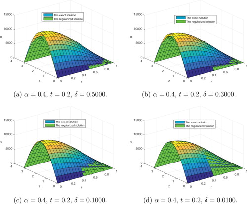
Table 1. The relative error in Figure 1.

δ	0.5000	0.3000	0.1000	0.0100
$e_r\left(\delta \right)$	0.1343	0.0807	0.0269	0.0027

Case 2. Now, we fix $\alpha =0.6$, b = 3.1, $\delta =0.1$. We take different values of t. We have Figure 2 and Table 2. Comparing Figure 1 with Figure 2, we find that when t becomes closer to zero, the rate at which the regularization converges to the exact solution slows down. This is consistent with our theoretical analysis.

Figure 2. The exact solution and the regularized solutions in Table 2. (a) $\alpha =0.6$, $\delta =0.1000$, t = 0.01. (b) $\alpha =0.6$, $\delta =0.1000$ , t = 0.05. (c) $\alpha =0.6$, $\delta =0.1000$, t = 0.5. (d) $\alpha =0.6$, $\delta =0.1000$, t = 0.8.

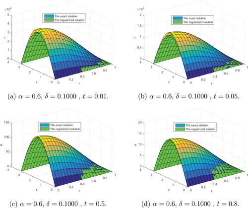
Table 2. The relative error in Figure 2.

t	0.01	0.05	0.5	0.8
$e_r\left(\delta \right)$	0.0900	0.0759	0.0333	0.0233

Case 3. Let b = 3.1, t = 0.6, $\delta =0.05$. We take different values of α. We have Figure 3 and Table 3. Figure 3 and Table 3 show that as the α is smaller, the error between the regularized solution and the exact solution decreases. Through numerical experiments, we find that the smaller α is, the better reconstruction result is. Finally, it should be noted that the value of b is determined after many numerical experiments. Although theoretically, when b is greater than or equal to 1, our method is convergent. But for the appropriate choice b, we will get faster convergence speed.

Figure 3. The exact solution and the regularized solutions in Table 3. (a) $\alpha =0.1$, t = 0.6, $\delta =0.05$. (b) $\alpha =0.3$, t = 0.6, $\delta =0.05$. (c) $\alpha =0.6$, t = 0.6, $\delta =0.05$. (d) $\alpha =1$, t = 0.6, $\delta =0.05$.

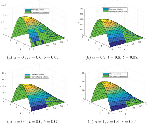
Table 3. The relative error in Figure 3.

α	0.1	0.3	0.6	1
$e_r\left(\delta \right)$	3.6488e-06	0.0029	0.0147	0.0274

6. Conclusion

In this paper, we study a backward problem for the inhomogeneous conformable fractional heat equation in a cylinder. We solve it by a modified quasi-boundary value method. we have established an error estimate between exact and regularized solutions. Corresponding to different levels of the smoothness of the exact solution, the convergence rates are improved gradually. Numerical examples show that our proposed regularization method is effective and stable.

Acknowledgements

We would like to thank the anonymous referees and the editor for valuable comments and helpful suggestions, which substantially improved the earlier version of the paper. This work is partially supported by the Natural Science Foundation of China (No 11661072), the Natural Science Foundation of Northwest Normal University, China (No NWNU-LKQN-17-5).

Disclosure statement

No potential conflict of interest was reported by the author(s).

Additional information

Funding

This work is partially supported by the the Natural Science Foundation of China [grant number No 11661072], the Natural Science Foundation of Northwest Normal University (NWNU), China [grant number NWNULKQN- 17-5].

References

- Magin RL. Fractional calculus models of complex dynamics in biological tissues. Computers Math Appl. 2010;59(5):1586–1593.
- Magin R, Ortigueira MD, Podlubny I, et al. On the fractional signals and systems. Signal Process. 2011;91(3):350–371.
- Meral FC, Royston TJ, Magin R. Fractional calculus in viscoelasticity: an experimental study. Commun Nonlinear Sci Numer Simul. 2010;15(4):939–945.
- Abbaszadeh M, Dehghan M. Analysis of mixed finite element method (MFEM) for solving the generalized fractional reaction-diffusion equation on nonrectangular domains. Computers Math Appl. 2019;78:1531–1547.
- Cheng Q, Xiong XT. An iterative method for an inverse source problem of a time-fractional diffusion equation. Math Numer Sin. 2017;39(3):295–308.
- Cheng W, Ma YJ, Fu CL. Identifying an unknown source term in radial heat conduction. Inverse Probl Sci Eng. 2012;20(3):335–349.
- Dehghan M, Abbaszadeh M. A Legendre spectral element method (SEM) based on the modified bases for solving neutral delay distributed-order fractional damped diffusion-wave equation. Math Methods Appl Sci. 2018;41(9):3476–3494.
- Dehghan M, Abbaszadeh M. A finite difference/finite element technique with error estimate for space fractional tempered diffusion-wave equation. Computers Math Appl. 2018;75(8):2903–2914.
- Tuan NH, Nane E. Inverse source problem for time-fractional diffusion with discrete random noise. Statist Probab Lett. 2017;120:126–134.
- Wei T, Li XL, Li YS. An inverse time-dependent source problem for a time-fractional diffusion equation. Inverse Probl. 2016;32(8):085003.
- Xiong XT, Ma XJ. A backward identification problem for an axis-symmetric fractional diffusion equation. Math Modelling and Anal. 2017;22(3):311–320.
- Zhang Y, Xu X. Inverse source problem for a fractional diffusion equation. Inverse Probl. 2011;27(3):035010.
- Khalil R, Al Horani M, Yousef A, et al. A new defnition of fractional derivative. J Comput Appl Math. 2014;264:65–70.
- Abdeljawad T. On conformable fractional calculus. J Comput Appl Math. 2014;279:57–66.
- Atangana A, Baleanu D, Alsaedi A. New properties of conformable derivative. Open Math. 2015;13:889–898.
- Anderson DR, Ulness DJ. Properties of the Katugampola fractional derivative with potential application in quantum mechanics. J Math Phys. 2015;56:063502. 18 pp.
- Zhao D, Luo M. General conformable fractional derivative and its physical interpretation. Calcolo. 2017;54(3):903–917.
- Liu CS. On the local fractional derivative of everywhere non-differentiable continuous functions on intervals. Commun Nonlinear Sci Numer Simul. 2017;42:229–235.
- Tarasov VE. No nonlocality. no fractional derivative. Commun Nonlinear Sci Numer Simul. 2018;62:157–163.
- Çenesiz Y, Kurt A, Nane E. Stochastic solutions of conformable fractional Cauchy problems. Stat Probab Lett. 2017;124:126–131.
- Çenesiz Y, Kurt A. The solutions of time and space conformable fractional heat equations with conformable Fourier transform. Acta Universitatis Sapientiae Math. 2015;7(2):130–140.
- Abu HI, Khalil R. Fractional Fourier series with applications. Am J Comput Appl Math. 2014;4(6):187–191.
- Avci D, Eroglu BBI, Ozdemir N. Conformable heat equation on a radial symmetric plate. Thermal Sci. 2017;21(2):819–826.
- Yavuz M, Ozdemir N. Numerical inverse Laplace homotopy technique for fractional heat equations. Thermal Sci. 2018;22(1):185–194.
- Vu H, O'Regan D, Van Hoa N. Regularization and error estimates for an inverse heat problem under the conformable derivative. Open Math. 2018;16(1):999–1011.
- Özkan O, Kurt A. On conformable double Laplace transform. Opt Quantum Electron. 2018;50(2):103. doi:10.1007/s11082-018-1372-9
- Nuruddeen RI, Zaman FD, Zakariya YF. Analysing the fractional heat diffusion equation solution in comparison with the new fractional derivative by decomposition method. Malaya J Matematik). 2019;7(2):213–222.
- Ali KK, Shaalan MA, Raslan KR. An extended theoretical and numerical study of two-Point boundary value problems using collocation method with physical applications. Numer Comput Meth Sci Eng. 2019;1(1):33–39.
- Raslan KR, Ali KK. Adomian decomposition method (ADM) for solving the nonlinear generalized regularized long wave equation. Numer Comput Meth Sci Eng. 2019;1(1):41–55.
- Rezazadeh H, Ali KK, Eslami M, et al. On the soliton solutions to the space-time fractional simplified MCH equation. J Interdisciplinary Math. 2019;22(2):149–165.
- Seadawy AR, Ali KK, Nuruddeen RI. A variety of soliton solutions for the fractional Wazwaz-Benjamin-Bona-Mahony equations. Results Phys. 2019;12:2234–2241.
- Souleymanou A, Ali KK, Rezazadeh H, et al. The propagation of waves in thin-film ferroelectric materials. Pramana. 2019;93(2):27.
- Taqi AH, Shallal MA, Jomaa BF, et al. Travelling wave solution for some partial differential equations. AIP Conf Proc. 2019;2096(1):020015.
- Tuan NH, Trong DD, Quan PH. Notes on a new approximate solution of 2-D heat equation backward in time. Appl Math Model. 2011;35:5673–5690.
- Eroğlu Bİ, Avcı D, Özdemir N. Optimal control problem for a conformable fractional heat conduction equation. Acta Phys Polonica A. 2017;132(3):658–662.