A local meshless procedure to determine the unknown control parameter in the multi-dimensional inverse problems

Abstract

This article is devoted to applying a local meshless method for specifying an unknown control parameter in one- and multi-dimensional inverse problems which are considered with a temperature overspecification condition at a specific point or an energy overspecification condition over the computational domain. Finding the unknowns in inverse problems is a challenge because these problems are modeled as non-classical parabolic problems and also have a significant role in describing physical phenomena of the real world. In this study, a combination of the meshless method of radial basis functions and finite difference method (called radial basis function-finite difference method) is used to solve inverse problems because this method has two important features. First it does not require any mesh generation. Consequently, it can be exerted to handle the high-dimensional inverse problems. Secondly, since this method is local, at each time step, a system with a sparse coefficient matrix is solved. Hence, the computational time and cost will be much low. Various numerical examples are examined, and also the accuracy and computational time required are presented. The numerical results indicate that the mentioned procedure is appropriate for the identification of the unknown parameter of inverse problems.

Keywords:

• Finite difference method
• local meshless method
• radial basis function-finite difference (RBF-FD) method
• inverse problem
• control parameter

AMS subject Classifications:

• 35R30
• 65L12
• 80M20
• 65M70

1. Introduction

Parabolic inverse problems play a fundamental role in modeling some physical phenomena. They emerge in various fields of physics and engineering such as analysis of heat conduction, thermoplasticity, chemical diffusion and control theory. Until now, specifying the unknown sources in inverse source problems has attracted a lot of attention. The applications of this kind of inverse problem have been extended to various fields of applied science such as identification of pollution sources in surface water [1–4], bio-luminescence tomography [5], electroencephalography[6], photo/optical tomography [7]. Hence, researchers and scientists have made great efforts to develop, analyze and implement numerical methods for the solution of these problems.

This article is devoted to the following inverse problem [8, 9] (1) $v_t(\mathbf{\text{x}},t)=\mathrm{\Delta }v(\mathbf{x},t)+p\left(t\right)v(\mathbf{x},t)+\varphi (\mathbf{x},t),(\mathbf{x},t)\in \mathrm{\Omega }\times (0,T],$(1) with initial and boundary conditions (2) $\begin{array}{rl}v(\mathbf{x},0)& =f\left(\mathbf{x}\right),\mathbf{x}\in \mathrm{\Omega },\end{array}$(2) (3) $\begin{array}{rl}v(\mathbf{x},t)& =g(\mathbf{x},t),(\mathbf{x},t)\in \mathrm{\partial }\mathrm{\Omega }\times (0,T],\end{array}$(3) subject to either a temperature overspecification condition at a precise point ${\mathbf{x}}^{\ast }$ in the computational domain (4) $v({\mathbf{\text{x}}}^{\ast },t)=E\left(t\right),t\in (0,T],{\mathbf{\text{x}}}^{\ast }\in \mathrm{\Omega },$(4) or to an energy overspecification over the computational domain (5) ${\int }_{\mathrm{\Omega }}k\left(\mathbf{\text{x}}\right)v(\mathbf{\text{x}},t)\mathrm{d}\mathbf{\text{x}}=E\left(t\right),t\in [0,T],$(5) where $\varphi (\mathbf{x},t),f\left(\mathbf{x}\right),g(\mathbf{x},t),k\left(\mathbf{x}\right)$ and $E\left(t\right)$ are known functions, while $v(\mathbf{x},t),$ and $p\left(t\right)$ are unknown functions.

The problem (1(1) $v_t(\mathbf{\text{x}},t)=\mathrm{\Delta }v(\mathbf{x},t)+p\left(t\right)v(\mathbf{x},t)+\varphi (\mathbf{x},t),(\mathbf{x},t)\in \mathrm{\Omega }\times (0,T],$(1) ) is translated as a heat transfer process with control function $p\left(t\right)$, assuming that $v(\mathbf{x},t)$ demonstrates the temperature distribution. Equation (4(4) $v({\mathbf{\text{x}}}^{\ast },t)=E\left(t\right),t\in (0,T],{\mathbf{\text{x}}}^{\ast }\in \mathrm{\Omega },$(4) ) determines the temperature at a specific point ${\mathbf{x}}^{\ast }$ in the computational domain at any time, and Equation (5(5) ${\int }_{\mathrm{\Omega }}k\left(\mathbf{\text{x}}\right)v(\mathbf{\text{x}},t)\mathrm{d}\mathbf{\text{x}}=E\left(t\right),t\in [0,T],$(5) ) represents thermal energy surrounded in a part of the computational domain. So, the purpose of solving Equation (1(1) $v_t(\mathbf{\text{x}},t)=\mathrm{\Delta }v(\mathbf{x},t)+p\left(t\right)v(\mathbf{x},t)+\varphi (\mathbf{x},t),(\mathbf{x},t)\in \mathrm{\Omega }\times (0,T],$(1) ) is to specify control parameter $p\left(t\right)$ that will represent a desired temperature at a specific point ${\mathbf{x}}^{\ast }$ or a desired thermal energy distribution in part of the computational domain [8,9].

The primary work done on the inverse problem is to prove the existence, uniqueness, and stability of their solutions [8, 10–14]. Then, many researchers concentrated on the inverse problem with a temperature overspecification condition (called the first inverse problem in current research). The authors of [15, 16] exerted various FD methods for solving 1-D first inverse problems. The authors of [17] described how to use the Legendre multiscaling basis approximation and Galerkin method for detecting the parameter $p\left(t\right)$ in the 1-D case. Article [18] is devoted to solving the 1-D case of Equation (1(1) $v_t(\mathbf{\text{x}},t)=\mathrm{\Delta }v(\mathbf{x},t)+p\left(t\right)v(\mathbf{x},t)+\varphi (\mathbf{x},t),(\mathbf{x},t)\in \mathrm{\Omega }\times (0,T],$(1) ) by a shifted Legendre tau method. In [19], the solution of Equation (1(1) $v_t(\mathbf{\text{x}},t)=\mathrm{\Delta }v(\mathbf{x},t)+p\left(t\right)v(\mathbf{x},t)+\varphi (\mathbf{x},t),(\mathbf{x},t)\in \mathrm{\Omega }\times (0,T],$(1) ) is approximated by Chebyshev cardinal functions in the 1-D case. Mohebbi and his co-worker [20] firstly discretized the spatial derivatives of Equation (1(1) $v_t(\mathbf{\text{x}},t)=\mathrm{\Delta }v(\mathbf{x},t)+p\left(t\right)v(\mathbf{x},t)+\varphi (\mathbf{x},t),(\mathbf{x},t)\in \mathrm{\Omega }\times (0,T],$(1) ) by a fourth-order compact method and they then employed the boundary value method for solving the obtained system of ordinary differential equations. The main targets of [21, 22] were to develop a meshless method for solving the 1-D Equation (1(1) $v_t(\mathbf{\text{x}},t)=\mathrm{\Delta }v(\mathbf{x},t)+p\left(t\right)v(\mathbf{x},t)+\varphi (\mathbf{x},t),(\mathbf{x},t)\in \mathrm{\Omega }\times (0,T],$(1) ). A greedy meshless local Petrov-Galerkin (MLPG) method was presented for determining the parameter $p\left(t\right)$ in 2-D inverse problems by Takhtabnoos and her co-worker [23]. Article [24] is devoted to solving the 3-D inverse problem with the overspecification condition at a specific point.

Also, various numerical methods are investigated for solving the inverse problem with the energy overspecification condition (called the second inverse problem in this investigation). Several FD schemes are applied for solving the 1-D Equation (1(1) $v_t(\mathbf{\text{x}},t)=\mathrm{\Delta }v(\mathbf{x},t)+p\left(t\right)v(\mathbf{x},t)+\varphi (\mathbf{x},t),(\mathbf{x},t)\in \mathrm{\Omega }\times (0,T],$(1) ) in [25, 26]. Wang and his co-author [27] employed the Crank-Nicolson finite difference (FD) method for finding the control parameter $p\left(t\right)$ in the 1-D case. Three finite difference schemes, $(1,5)$ fully explicit technique, $(5,5)$ Noye-Hayman fully implicit scheme and Peaceman-Rachford alternating direction implicit (P-R ADI) methods are extended to solve the 2-D case of Equation (1(1) $v_t(\mathbf{\text{x}},t)=\mathrm{\Delta }v(\mathbf{x},t)+p\left(t\right)v(\mathbf{x},t)+\varphi (\mathbf{x},t),(\mathbf{x},t)\in \mathrm{\Omega }\times (0,T],$(1) ). These methods have second-order accuracy but it is shown that the P-R ADI scheme is more efficient and has less computational time than the rest [9]. The author of [28] used various fourth-order methods for the 1-D problem (1(1) $v_t(\mathbf{\text{x}},t)=\mathrm{\Delta }v(\mathbf{x},t)+p\left(t\right)v(\mathbf{x},t)+\varphi (\mathbf{x},t),(\mathbf{x},t)\in \mathrm{\Omega }\times (0,T],$(1) )–(3(3) $\begin{array}{rl}v(\mathbf{x},t)& =g(\mathbf{x},t),(\mathbf{x},t)\in \mathrm{\partial }\mathrm{\Omega }\times (0,T],\end{array}$(3) ) with the integral overspecification condition (5(5) ${\int }_{\mathrm{\Omega }}k\left(\mathbf{\text{x}}\right)v(\mathbf{\text{x}},t)\mathrm{d}\mathbf{\text{x}}=E\left(t\right),t\in [0,T],$(5) ). In [24, 29], the 3-D inverse problem with the energy overspecification condition is solved by a FD scheme and a Legendre pseudo-spectral method, respectively.

The RBF-FD method seems to have been first proposed by Tolstykh via a conference presentation in 2000 in [30]. In [31], it has been noted that when $ϵ\to 0$, the convergence of RBF interpolants to polynomial would propose RBF-generated finite difference methods. Moreover, in 2002, Wang and his co-worker presented some RBF-FD applications in Ref. [32]. Finally, in 2003, the RBF-FD method is applied for solving two-dimensional incompressible Navier-Stokes equations [33]. Authors of [34] implemented the RBF-FD and LSFD methods for 2-D Poisson and Lid-Driven equations. Besides, they indicated that the RBF-FD method has significant accuracy. The main aim of [35] is to use the RBF-FD method for solving steady convection-diffusion equations. In [36], it has been explained how to apply the RBF-FD method to the shallow water equations and also the accuracy and computational efficiency of the mentioned method have been established. Bolling et al. [37] were the first researchers to concentrate on the parallel performance of the RBF-FD method and presented parallelization strategies. In [38] the RBF-FD method has been applied for solving 2-D Navier-Stokes equation. Moreover, an adaptive shape parameter for RBFs has been presented in order to improve numerical results. In Ref. [39], the RBF-FD is applied for the simulation of some models in the nonlinear wave phenomena such as the regularized long-wave and Extended Fisher-Kolmogorov equations in one-, two- and three- dimensional cases.

1.1. The main structure of this article

This study is dedicated to applying the RBF-FD method for solving the problem (1(1) $v_t(\mathbf{\text{x}},t)=\mathrm{\Delta }v(\mathbf{x},t)+p\left(t\right)v(\mathbf{x},t)+\varphi (\mathbf{x},t),(\mathbf{x},t)\in \mathrm{\Omega }\times (0,T],$(1) )–(3(3) $\begin{array}{rl}v(\mathbf{x},t)& =g(\mathbf{x},t),(\mathbf{x},t)\in \mathrm{\partial }\mathrm{\Omega }\times (0,T],\end{array}$(3) ) subject to the overspacification condition (4(4) $v({\mathbf{\text{x}}}^{\ast },t)=E\left(t\right),t\in (0,T],{\mathbf{\text{x}}}^{\ast }\in \mathrm{\Omega },$(4) ) or (5(5) ${\int }_{\mathrm{\Omega }}k\left(\mathbf{\text{x}}\right)v(\mathbf{\text{x}},t)\mathrm{d}\mathbf{\text{x}}=E\left(t\right),t\in [0,T],$(5) ). The framework of this paper is as follow:

• In Section 2, a general description of the RBF-FD scheme is presented.

• Section 3 is devoted to the elaboration of linearization of inverse problems.

• In Section 4, we account for how to implement the RBF-FD technique for one- and multi-dimensional first linearized inverse problems.

• Section 5 relates to applying the RBF-FD technique for one- and multi-dimensional second linearized inverse problems.

• In Section 6, we consider several numerical results to simulate the RBF-FD method for solving one- and multi-dimensional inverse problems.

• Section 7 provides the overall conclusion of this research.

2. A general description on the RBF-FD method

FD formulas for a regular mesh are generally derived from 1-D case. To obtain FD formulas in high dimension in Cartesian grids, the 1-D FD can be separately employed in each spatial direction. Now, the main goal is to find a polynomial-based FD-formula. There are various approaches for detecting the weights in 1-D FD formulas. The simplest of them is that the formulas must be precise for the monomials $1,x,x^2,\dots$ up to the highest degree possible [40, 41]. For instance, we approximate the linear differential operator $\mathcal{L}$ at the point $x_c$ with $n_s$ points over its stencil. Hence, the unknowns $x_c$-related are determined by solving the following linear system [40] (6) $\underset{\mathbf{V}}{\underbrace{\left[\begin{array}{ccccc}1& 1& 1& \dots & 1\\ x_1& x_2& x_3& \dots & x_{n_s}\\ x_1^2& x_2^2& x_3^2& \dots & x_{n_s}^2\\ ⋮& ⋮& ⋮& \ddots & ⋮\\ x_1^{n-1}& x_2^{n-1}& x_3^{n-1}& \cdots & x_{n_s}^{n_s-1}\end{array}\right]}}\left[\begin{array}{c}{\xi }_1\\ {\xi }_2\\ {\xi }_3\\ ⋮\\ {\xi }_{n_s}\end{array}\right]=\left[\begin{array}{c}\mathcal{L}\left(1\right){|}_{x=x_c}\\ \mathcal{L}\left(x\right){|}_{x=x_c}\\ \mathcal{L}\left(x^2\right){|}_{x=x_c}\\ ⋮\\ \mathcal{L}\left(x^{n_s-1}\right){|}_{x=x_c}\end{array}\right].$(6) The Vandermonde matrix $\mathbf{V}$ is nonsingular if the points $x_i$ are distinct. This approach is not applicable to scattered points and multivariate functions because the unisolvency feature does not resolve in this case [40].

The main concept in finding a radial basis function-generated finite difference (RBF-FD) formula is to use d-D RBFs ($d\ge 1$) centered at ${\tilde{x}}_i$, $i=1,2,\dots ,n_s$ instead of the monomial functions in the system (6(6) $\underset{\mathbf{V}}{\underbrace{\left[\begin{array}{ccccc}1& 1& 1& \dots & 1\\ x_1& x_2& x_3& \dots & x_{n_s}\\ x_1^2& x_2^2& x_3^2& \dots & x_{n_s}^2\\ ⋮& ⋮& ⋮& \ddots & ⋮\\ x_1^{n-1}& x_2^{n-1}& x_3^{n-1}& \cdots & x_{n_s}^{n_s-1}\end{array}\right]}}\left[\begin{array}{c}{\xi }_1\\ {\xi }_2\\ {\xi }_3\\ ⋮\\ {\xi }_{n_s}\end{array}\right]=\left[\begin{array}{c}\mathcal{L}\left(1\right){|}_{x=x_c}\\ \mathcal{L}\left(x\right){|}_{x=x_c}\\ \mathcal{L}\left(x^2\right){|}_{x=x_c}\\ ⋮\\ \mathcal{L}\left(x^{n_s-1}\right){|}_{x=x_c}\end{array}\right].$(6) ). Therefore, it leads to the following system for the approximation of any linear operator (7) $\begin{array}{rl}& \underbrace{{\left[\begin{array}{cccc}\mathrm{\Psi }(\parallel {\tilde{x}}_1-{\tilde{x}}_1\parallel )& \mathrm{\Psi }(\parallel {\tilde{x}}_2-{\tilde{x}}_1\parallel )& \dots & \mathrm{\Psi }(\parallel {\tilde{x}}_{n_s}-{\tilde{x}}_1\parallel )\\ \mathrm{\Psi }(\parallel {\tilde{x}}_1-{\tilde{x}}_2\parallel )& \mathrm{\Psi }(\parallel {\tilde{x}}_2-{\tilde{x}}_2\parallel )& \cdots & \mathrm{\Psi }(\parallel {\tilde{x}}_{n_s}-{\tilde{x}}_2\parallel )\\ ⋮& ⋮& \ddots & ⋮\\ \mathrm{\Psi }(\parallel {\tilde{x}}_1-{\tilde{x}}_{n_s}\parallel )& \mathrm{\Psi }(\parallel {\tilde{x}}_2-{\tilde{x}}_{n_s}\parallel )& \cdots & \mathrm{\Psi }(\parallel {\tilde{x}}_{n_s}-{\tilde{x}}_{n_s}\parallel )\end{array}\right]}_{\mathbf{A}}}\left[\begin{array}{c}{\xi }_1\\ {\xi }_2\\ ⋮\\ {\xi }_{n_s}\end{array}\right]\\ & =\left[\begin{array}{c}\mathcal{L}\mathrm{\Psi }(\parallel \tilde{x}-{\tilde{x}}_1\parallel ){|}_{\tilde{x}={\tilde{x}}_c}\\ \mathcal{L}\mathrm{\Psi }(\parallel \tilde{x}-{\tilde{x}}_2\parallel ){|}_{{}_{\tilde{x}={\tilde{x}}_c}}\\ ⋮\\ \mathcal{L}\mathrm{\Psi }(\parallel \tilde{x}-{\tilde{x}}_n\parallel ){|}_{{}_{\tilde{x}={\tilde{x}}_c}}\end{array}\right],\end{array}$(7) where $\parallel .\parallel$ denotes the common Euclidean norm. The invertibility of matrix $\mathbf{A}$ is guaranteed when RBFs are selected from Table 1 [42].

Table 1. Definition of several radial functions [42, 43]

Title of function	Radial function
Gaussian	$\mathrm{\Psi }\left(r\right)=\exp (-(\eta r{)}^2)$
Multiquadric	$\mathrm{\Psi }\left(r\right)=(1+(\eta r{)}^2{)}^{1/2}$
Inverse Multiquadric	$\mathrm{\Psi }\left(r\right)=(1+(\eta r{)}^2{)}^{-1/2}$
Inverse quadratic	$\mathrm{\Psi }\left(r\right)=(1+(\eta r{)}^2{)}^{-1}$

The matrix $\mathbf{A}$ in the system (7(7) $\begin{array}{rl}& \underbrace{{\left[\begin{array}{cccc}\mathrm{\Psi }(\parallel {\tilde{x}}_1-{\tilde{x}}_1\parallel )& \mathrm{\Psi }(\parallel {\tilde{x}}_2-{\tilde{x}}_1\parallel )& \dots & \mathrm{\Psi }(\parallel {\tilde{x}}_{n_s}-{\tilde{x}}_1\parallel )\\ \mathrm{\Psi }(\parallel {\tilde{x}}_1-{\tilde{x}}_2\parallel )& \mathrm{\Psi }(\parallel {\tilde{x}}_2-{\tilde{x}}_2\parallel )& \cdots & \mathrm{\Psi }(\parallel {\tilde{x}}_{n_s}-{\tilde{x}}_2\parallel )\\ ⋮& ⋮& \ddots & ⋮\\ \mathrm{\Psi }(\parallel {\tilde{x}}_1-{\tilde{x}}_{n_s}\parallel )& \mathrm{\Psi }(\parallel {\tilde{x}}_2-{\tilde{x}}_{n_s}\parallel )& \cdots & \mathrm{\Psi }(\parallel {\tilde{x}}_{n_s}-{\tilde{x}}_{n_s}\parallel )\end{array}\right]}_{\mathbf{A}}}\left[\begin{array}{c}{\xi }_1\\ {\xi }_2\\ ⋮\\ {\xi }_{n_s}\end{array}\right]\\ & =\left[\begin{array}{c}\mathcal{L}\mathrm{\Psi }(\parallel \tilde{x}-{\tilde{x}}_1\parallel ){|}_{\tilde{x}={\tilde{x}}_c}\\ \mathcal{L}\mathrm{\Psi }(\parallel \tilde{x}-{\tilde{x}}_2\parallel ){|}_{{}_{\tilde{x}={\tilde{x}}_c}}\\ ⋮\\ \mathcal{L}\mathrm{\Psi }(\parallel \tilde{x}-{\tilde{x}}_n\parallel ){|}_{{}_{\tilde{x}={\tilde{x}}_c}}\end{array}\right],\end{array}$(7) ) is known as the RBF interpolation matrix. Suppose a set of distributed points ${\tilde{x}}_j\in \mathrm{\Omega }$ and function values $f\left({\tilde{x}}_j\right)$ ($j=1,\dots ,N$) are given, then the local RBF interpolant is introduced as [40] (8) $\mathcal{I}\left(\tilde{x}\right)=\sum _{i=1}^{n_s}{\gamma }_i\mathrm{\Psi }\left(∥\tilde{x}-{\tilde{x}}_i∥\right).$(8)

By enforcing the interpolation conditions, the unknowns $\{{\gamma }_i{\}}_{i=1}^{n_s}$ are obtained by solving $\mathbf{A}\overrightarrow{\mathit{\gamma }}=\mathbf{f}$.

RBFs are employed to approximate derivative operators in two different cases, global and local. In the former, the number of points inside each stencil $n_s$ is equal to the total number of points N in the computational domain while in the latter, the number of points inside each stencil $n_s$ is much less than the total number of points N. For simplicity, the RBF-FD stencil over any point consists of its $n_s$ nearest points.

The approximation of linear operator $\mathcal{L}$ around each point requires a $n_s$-set of weights that are obtained by solving the system of (7(7) $\begin{array}{rl}& \underbrace{{\left[\begin{array}{cccc}\mathrm{\Psi }(\parallel {\tilde{x}}_1-{\tilde{x}}_1\parallel )& \mathrm{\Psi }(\parallel {\tilde{x}}_2-{\tilde{x}}_1\parallel )& \dots & \mathrm{\Psi }(\parallel {\tilde{x}}_{n_s}-{\tilde{x}}_1\parallel )\\ \mathrm{\Psi }(\parallel {\tilde{x}}_1-{\tilde{x}}_2\parallel )& \mathrm{\Psi }(\parallel {\tilde{x}}_2-{\tilde{x}}_2\parallel )& \cdots & \mathrm{\Psi }(\parallel {\tilde{x}}_{n_s}-{\tilde{x}}_2\parallel )\\ ⋮& ⋮& \ddots & ⋮\\ \mathrm{\Psi }(\parallel {\tilde{x}}_1-{\tilde{x}}_{n_s}\parallel )& \mathrm{\Psi }(\parallel {\tilde{x}}_2-{\tilde{x}}_{n_s}\parallel )& \cdots & \mathrm{\Psi }(\parallel {\tilde{x}}_{n_s}-{\tilde{x}}_{n_s}\parallel )\end{array}\right]}_{\mathbf{A}}}\left[\begin{array}{c}{\xi }_1\\ {\xi }_2\\ ⋮\\ {\xi }_{n_s}\end{array}\right]\\ & =\left[\begin{array}{c}\mathcal{L}\mathrm{\Psi }(\parallel \tilde{x}-{\tilde{x}}_1\parallel ){|}_{\tilde{x}={\tilde{x}}_c}\\ \mathcal{L}\mathrm{\Psi }(\parallel \tilde{x}-{\tilde{x}}_2\parallel ){|}_{{}_{\tilde{x}={\tilde{x}}_c}}\\ ⋮\\ \mathcal{L}\mathrm{\Psi }(\parallel \tilde{x}-{\tilde{x}}_n\parallel ){|}_{{}_{\tilde{x}={\tilde{x}}_c}}\end{array}\right],\end{array}$(7) ). A differentiation matrix is formed by replacing the obtained weight sets in its consecutive rows. To determine the rows of this matrix, we use the system (7(7) $\begin{array}{rl}& \underbrace{{\left[\begin{array}{cccc}\mathrm{\Psi }(\parallel {\tilde{x}}_1-{\tilde{x}}_1\parallel )& \mathrm{\Psi }(\parallel {\tilde{x}}_2-{\tilde{x}}_1\parallel )& \dots & \mathrm{\Psi }(\parallel {\tilde{x}}_{n_s}-{\tilde{x}}_1\parallel )\\ \mathrm{\Psi }(\parallel {\tilde{x}}_1-{\tilde{x}}_2\parallel )& \mathrm{\Psi }(\parallel {\tilde{x}}_2-{\tilde{x}}_2\parallel )& \cdots & \mathrm{\Psi }(\parallel {\tilde{x}}_{n_s}-{\tilde{x}}_2\parallel )\\ ⋮& ⋮& \ddots & ⋮\\ \mathrm{\Psi }(\parallel {\tilde{x}}_1-{\tilde{x}}_{n_s}\parallel )& \mathrm{\Psi }(\parallel {\tilde{x}}_2-{\tilde{x}}_{n_s}\parallel )& \cdots & \mathrm{\Psi }(\parallel {\tilde{x}}_{n_s}-{\tilde{x}}_{n_s}\parallel )\end{array}\right]}_{\mathbf{A}}}\left[\begin{array}{c}{\xi }_1\\ {\xi }_2\\ ⋮\\ {\xi }_{n_s}\end{array}\right]\\ & =\left[\begin{array}{c}\mathcal{L}\mathrm{\Psi }(\parallel \tilde{x}-{\tilde{x}}_1\parallel ){|}_{\tilde{x}={\tilde{x}}_c}\\ \mathcal{L}\mathrm{\Psi }(\parallel \tilde{x}-{\tilde{x}}_2\parallel ){|}_{{}_{\tilde{x}={\tilde{x}}_c}}\\ ⋮\\ \mathcal{L}\mathrm{\Psi }(\parallel \tilde{x}-{\tilde{x}}_n\parallel ){|}_{{}_{\tilde{x}={\tilde{x}}_c}}\end{array}\right],\end{array}$(7) ) to earn all weights sets at each point. Hence, the weights of $x_k$-point are obtained as follows [40] (9) $\left({\overrightarrow{\xi }}_k\right)={\mathbf{\text{{A}}}}^{-1}\overrightarrow{h},$(9) where ${\mathbf{A}}_{ij}=\mathrm{\Psi }(\parallel {\tilde{x}}_j-{\tilde{x}}_i\parallel )$ and $(h{)}_i=\mathcal{L}\mathrm{\Psi }(\parallel \tilde{x}-{\tilde{x}}_i\parallel ){|}_{\tilde{x}={\tilde{x}}_k}$. Then, the computed weights ${\overrightarrow{\xi }}_k$ must be set in the $k^{th}$ row of the differentiation matrix $\mathcal{D}$. Finally, any linear differential operator is approximated as (10) $\left[\begin{array}{c}\mathcal{L}f\left(\hat{x}\right){|}_{x=x_1}\\ ⋮\\ \mathcal{L}f\left(\hat{x}\right){|}_{x=x_N}\end{array}\right]\approx \mathcal{D}\left[\begin{array}{c}f\left({\hat{x}}_1\right)\\ ⋮\\ f\left({\hat{x}}_N\right)\end{array}\right].$(10) The resulting RBF-FD differentiation matrix $\mathcal{D}$ is a sparse matrix with the $n_s$ non-zero entries at any N rows. We present Algorithm 2 to explain how to construct a second-order differentiation matrix ${\mathcal{D}}^{xx}$. It should be noted that we use the Multiquadric radial function introduced in Table 1 and choose the suitable shape parameter η using Algorithm 1 which has been presented in [44].

The required parameters for Algorithm 1 are defined as :

1. $\mathbf{A}$ denotes the interpolation matrix.

2. ${\mathit{\sigma }}_{min}$ and ${\mathit{\sigma }}_{max}$, which are the smallest and largest singular values, are obtained from the singular-value decomposition (SVD).

3. ${\mathrm{K}}_{min}={10}^2$ and ${\mathrm{K}}_{max}={10}^4.$

4. $\overline{\mathit{\eta }}={\displaystyle \frac{1}{N}}.$

3. Linearization of inverse equation

The first aim is to linearize the non-linear Equation (1(1) $v_t(\mathbf{\text{x}},t)=\mathrm{\Delta }v(\mathbf{x},t)+p\left(t\right)v(\mathbf{x},t)+\varphi (\mathbf{x},t),(\mathbf{x},t)\in \mathrm{\Omega }\times (0,T],$(1) ) by using the following relations [9] (11) $w\left(t\right)=\exp \left(-{\int }_0^{t}p\left(\tau \right)\mathrm{d}\tau \right),u(\mathbf{x},t)=w\left(t\right)v(\mathbf{x},t).$(11) According to transformations (11(11) $w\left(t\right)=\exp \left(-{\int }_0^{t}p\left(\tau \right)\mathrm{d}\tau \right),u(\mathbf{x},t)=w\left(t\right)v(\mathbf{x},t).$(11) ), the unknown functions can be written as [9] (12) $v(\mathbf{x},t)=\frac{u(\mathbf{x},t)}{w\left(t\right)},p\left(t\right)=-\frac{w^{\prime }\left(t\right)}{w\left(t\right)}.$(12) Substituting (12(12) $v(\mathbf{x},t)=\frac{u(\mathbf{x},t)}{w\left(t\right)},p\left(t\right)=-\frac{w^{\prime }\left(t\right)}{w\left(t\right)}.$(12) ) in (1(1) $v_t(\mathbf{\text{x}},t)=\mathrm{\Delta }v(\mathbf{x},t)+p\left(t\right)v(\mathbf{x},t)+\varphi (\mathbf{x},t),(\mathbf{x},t)\in \mathrm{\Omega }\times (0,T],$(1) )–(5(5) ${\int }_{\mathrm{\Omega }}k\left(\mathbf{\text{x}}\right)v(\mathbf{\text{x}},t)\mathrm{d}\mathbf{\text{x}}=E\left(t\right),t\in [0,T],$(5) ), we obtain (13) $\begin{array}{rl}{u}_t(\mathbf{\text{x}},t)& =\mathrm{\Delta }u(\mathbf{x},t)+w\left(t\right)\varphi (\mathbf{x},t),(\mathbf{x},t)\in \mathrm{\Omega }\times [0,T],\\ u(\mathbf{x},0)& =f\left(\mathbf{x}\right),\mathbf{x}\in \mathrm{\Omega },\\ u(\mathbf{x},t)& =w\left(t\right)g(\mathbf{x},t),(\mathbf{x},t)\in \mathrm{\partial }\mathrm{\Omega }\times [0,T],\end{array}$(13) with temperature overspecification condition (14) $u({\mathbf{x}}^{\ast },t)=w\left(t\right)E\left(t\right),t\in [0,T],$(14) and energy overspecification condition (15) ${\int }_{\mathrm{\Omega }}k\left(\mathbf{\text{x}}\right)u(\mathbf{\text{x}},t)\mathrm{d}\mathbf{\text{x}}=w\left(t\right)E\left(t\right).$(15) Equations (14(14) $u({\mathbf{x}}^{\ast },t)=w\left(t\right)E\left(t\right),t\in [0,T],$(14) ) and (15(15) ${\int }_{\mathrm{\Omega }}k\left(\mathbf{\text{x}}\right)u(\mathbf{\text{x}},t)\mathrm{d}\mathbf{\text{x}}=w\left(t\right)E\left(t\right).$(15) ) are respectively equivalent to (16) $w\left(t\right)=\frac{u({\mathbf{\text{x}}}^{\ast },t)}{E\left(t\right)},w\left(t\right)=\frac{1}{E\left(t\right)}{\int }_{\mathrm{\Omega }}k\left(\mathbf{\text{x}}\right)u(\mathbf{\text{x}},t)d\mathbf{\text{x}},$(16) in which $E\left(t\right)\ne 0$. According to the two relations in (16(16) $w\left(t\right)=\frac{u({\mathbf{\text{x}}}^{\ast },t)}{E\left(t\right)},w\left(t\right)=\frac{1}{E\left(t\right)}{\int }_{\mathrm{\Omega }}k\left(\mathbf{\text{x}}\right)u(\mathbf{\text{x}},t)d\mathbf{\text{x}},$(16) ) for $w\left(t\right)$, we can deduce two new non-standard parabolic PDEs as follows [9]:

• First linearized inverse problem: By substituting the first values of $w\left(t\right)$ introduced in Equation (16(16) $w\left(t\right)=\frac{u({\mathbf{\text{x}}}^{\ast },t)}{E\left(t\right)},w\left(t\right)=\frac{1}{E\left(t\right)}{\int }_{\mathrm{\Omega }}k\left(\mathbf{\text{x}}\right)u(\mathbf{\text{x}},t)d\mathbf{\text{x}},$(16) ) in the problem (13(13) $\begin{array}{rl}{u}_t(\mathbf{\text{x}},t)& =\mathrm{\Delta }u(\mathbf{x},t)+w\left(t\right)\varphi (\mathbf{x},t),(\mathbf{x},t)\in \mathrm{\Omega }\times [0,T],\\ u(\mathbf{x},0)& =f\left(\mathbf{x}\right),\mathbf{x}\in \mathrm{\Omega },\\ u(\mathbf{x},t)& =w\left(t\right)g(\mathbf{x},t),(\mathbf{x},t)\in \mathrm{\partial }\mathrm{\Omega }\times [0,T],\end{array}$(13) ), the linearized form of the problem (1(1) $v_t(\mathbf{\text{x}},t)=\mathrm{\Delta }v(\mathbf{x},t)+p\left(t\right)v(\mathbf{x},t)+\varphi (\mathbf{x},t),(\mathbf{x},t)\in \mathrm{\Omega }\times (0,T],$(1) )–(4(4) $v({\mathbf{\text{x}}}^{\ast },t)=E\left(t\right),t\in (0,T],{\mathbf{\text{x}}}^{\ast }\in \mathrm{\Omega },$(4) ) is obtained [28] (117) $\begin{array}{rl}{u}_t(\mathbf{\text{x}},t)& =\mathrm{\Delta }u(\mathbf{x},t)+\frac{u({\mathbf{x}}^{\ast },t)}{E\left(t\right)}\varphi (\mathbf{x},t),(\mathbf{x},t)\in \mathrm{\Omega }\times [0,T],\end{array}$(117) (18) $\begin{array}{rl}u(\mathbf{x},0)& =f\left(\mathbf{x}\right),\mathbf{x}\in \mathrm{\Omega },\end{array}$(18) (19) $\begin{array}{rl}u(\mathbf{x},t)& -\frac{u({\mathbf{x}}^{\ast },t)}{E\left(t\right)}g(\mathbf{x},t)=0,(\mathbf{x},t)\in \mathrm{\partial }\mathrm{\Omega }\times [0,T].\end{array}$(19)

• Second linearized inverse problem:

  On the other hand, considering the second relation of $w\left(t\right)$ in (16(16) $w\left(t\right)=\frac{u({\mathbf{\text{x}}}^{\ast },t)}{E\left(t\right)},w\left(t\right)=\frac{1}{E\left(t\right)}{\int }_{\mathrm{\Omega }}k\left(\mathbf{\text{x}}\right)u(\mathbf{\text{x}},t)d\mathbf{\text{x}},$(16) ), the original problem (1(1) $v_t(\mathbf{\text{x}},t)=\mathrm{\Delta }v(\mathbf{x},t)+p\left(t\right)v(\mathbf{x},t)+\varphi (\mathbf{x},t),(\mathbf{x},t)\in \mathrm{\Omega }\times (0,T],$(1) )–(3(3) $\begin{array}{rl}v(\mathbf{x},t)& =g(\mathbf{x},t),(\mathbf{x},t)\in \mathrm{\partial }\mathrm{\Omega }\times (0,T],\end{array}$(3) ) with the energy overspecification condition (5(5) ${\int }_{\mathrm{\Omega }}k\left(\mathbf{\text{x}}\right)v(\mathbf{\text{x}},t)\mathrm{d}\mathbf{\text{x}}=E\left(t\right),t\in [0,T],$(5) ) is transformed into the following linear problem [24,26] (20) $\begin{array}{rl}& u_t(\mathbf{\text{x}},t)=\mathrm{\Delta }u(\mathbf{\text{x}},t)+\frac{\varphi (\mathbf{\text{x}},t)}{E\left(t\right)}{\int }_{\mathrm{\Omega }}k\left(\mathbf{\text{x}}\right)u(\mathbf{\text{x}},t)\mathrm{d}\mathbf{\text{x}},(\mathbf{\text{x}},t)\in \mathrm{\Omega }\times [0,T],\end{array}$(20) (21) $\begin{array}{rl}& u(\mathbf{\text{x}},0)=f\left(\mathbf{\text{x}}\right),\mathbf{x}\in \mathrm{\Omega },\end{array}$(21) (22) $\begin{array}{rl}& u(\mathbf{\text{x}},t)-\frac{g(\mathbf{\text{x}},t)}{E\left(t\right)}{\int }_{\mathrm{\Omega }}k\left(\mathbf{\text{x}}\right)u(\mathbf{\text{x}},t)\mathrm{d}\mathbf{\text{x}}=0,(\mathbf{\text{x}},t)\in \mathrm{\partial }\mathrm{\Omega }\times [0,T].\end{array}$(22)

Now, after obtaining the approximate solution of the problem (17(117) $\begin{array}{rl}{u}_t(\mathbf{\text{x}},t)& =\mathrm{\Delta }u(\mathbf{x},t)+\frac{u({\mathbf{x}}^{\ast },t)}{E\left(t\right)}\varphi (\mathbf{x},t),(\mathbf{x},t)\in \mathrm{\Omega }\times [0,T],\end{array}$(117) )–(19(19) $\begin{array}{rl}u(\mathbf{x},t)& -\frac{u({\mathbf{x}}^{\ast },t)}{E\left(t\right)}g(\mathbf{x},t)=0,(\mathbf{x},t)\in \mathrm{\partial }\mathrm{\Omega }\times [0,T].\end{array}$(19) ) or the problem (20(20) $\begin{array}{rl}& u_t(\mathbf{\text{x}},t)=\mathrm{\Delta }u(\mathbf{\text{x}},t)+\frac{\varphi (\mathbf{\text{x}},t)}{E\left(t\right)}{\int }_{\mathrm{\Omega }}k\left(\mathbf{\text{x}}\right)u(\mathbf{\text{x}},t)\mathrm{d}\mathbf{\text{x}},(\mathbf{\text{x}},t)\in \mathrm{\Omega }\times [0,T],\end{array}$(20) )–(22(22) $\begin{array}{rl}& u(\mathbf{\text{x}},t)-\frac{g(\mathbf{\text{x}},t)}{E\left(t\right)}{\int }_{\mathrm{\Omega }}k\left(\mathbf{\text{x}}\right)u(\mathbf{\text{x}},t)\mathrm{d}\mathbf{\text{x}}=0,(\mathbf{\text{x}},t)\in \mathrm{\partial }\mathrm{\Omega }\times [0,T].\end{array}$(22) ), access to the functions $v(\mathbf{x},t)$ and $p\left(t\right)$ is possible [24,28] with the following relations $\begin{array}{rl}v(\mathbf{x},t)& =\frac{E\left(t\right)}{u({\mathbf{x}}^{\ast },t)}u(\mathbf{x},t),\\ p\left(t\right)& =\frac{1}{E\left(t\right)}\left(E^{\prime }\left(t\right)-\mathrm{\Delta }v({\mathbf{x}}^{\ast },t)-\varphi ({\mathbf{x}}^{\ast },t)\right).\end{array}$

4. Discretization of the first linearized inverse problem

To discretize the time variable of Equation (17(117) $\begin{array}{rl}{u}_t(\mathbf{\text{x}},t)& =\mathrm{\Delta }u(\mathbf{x},t)+\frac{u({\mathbf{x}}^{\ast },t)}{E\left(t\right)}\varphi (\mathbf{x},t),(\mathbf{x},t)\in \mathrm{\Omega }\times [0,T],\end{array}$(117) ), it is necessary to consider the following. The time step is defined as $t_m=m\tau ,m=0,1,\dots ,N_t,$in which $\tau ={\displaystyle \frac{T}{N_t}}$ is the size of the time step. In this section, we employ a finite-difference scheme for the approximation of the first-order time derivative in Equation (17(117) $\begin{array}{rl}{u}_t(\mathbf{\text{x}},t)& =\mathrm{\Delta }u(\mathbf{x},t)+\frac{u({\mathbf{x}}^{\ast },t)}{E\left(t\right)}\varphi (\mathbf{x},t),(\mathbf{x},t)\in \mathrm{\Omega }\times [0,T],\end{array}$(117) ) as follows (23) $u^{n+1}\left(\mathbf{x}\right)-\frac{\tau }{2}\mathrm{\Delta }{u}^{n+1}\left(\mathbf{x}\right)=u^n\left(\mathbf{x}\right)+\frac{\tau }{2}\mathrm{\Delta }{u}^n\left(\mathbf{x}\right)+\frac{\tau }{E^n}{u}^n\left({\mathbf{x}}^{\ast }\right){\varphi }^n\left(\mathbf{x}\right),n=0,1,\dots ,N_t-1,$(23) where $u^n\left(\mathbf{x}\right)=u(\mathbf{x},t^n)$, ${\varphi }^n\left(\mathbf{x}\right)=\varphi (\mathbf{x},t^n)$. In the subsequent subsections, the spatial variable in Equation (23(23) $u^{n+1}\left(\mathbf{x}\right)-\frac{\tau }{2}\mathrm{\Delta }{u}^{n+1}\left(\mathbf{x}\right)=u^n\left(\mathbf{x}\right)+\frac{\tau }{2}\mathrm{\Delta }{u}^n\left(\mathbf{x}\right)+\frac{\tau }{E^n}{u}^n\left({\mathbf{x}}^{\ast }\right){\varphi }^n\left(\mathbf{x}\right),n=0,1,\dots ,N_t-1,$(23) ) is discretized with the radial basis function-generated finite difference (RBF-FD) method.

4.1. One-dimensional case

We next describe the implementation of the standard RBF-FD technique for solving the 1-D of the inverse problem. Suppose the computational domain is $\mathrm{\Omega }=[a,b]$. The 1-D semi-discrete case of the first inverse problem is (24) $u^{n+1}\left(x\right)-\frac{\tau }{2}{u}_{xx}^{n+1}\left(x\right)=u^n\left(x\right)+\frac{\tau }{2}{u}_{xx}^n\left(x\right)+\frac{\tau }{E^n}{u}^n\left({\mathbf{\text{x}}}^{\ast }\right){\varphi }^n\left(x\right).$(24) Collocating Equation (24(24) $u^{n+1}\left(x\right)-\frac{\tau }{2}{u}_{xx}^{n+1}\left(x\right)=u^n\left(x\right)+\frac{\tau }{2}{u}_{xx}^n\left(x\right)+\frac{\tau }{E^n}{u}^n\left({\mathbf{\text{x}}}^{\ast }\right){\varphi }^n\left(x\right).$(24) ) at the points $\{x_i{\}}_{i=1}^N$ yields $u^{n+1}\left(x_i\right)-\frac{\tau }{2}{u}_{xx}^{n+1}\left(x_i\right)=u^n\left(x_i\right)+\frac{\tau }{2}{u}_{xx}^n\left(x_i\right)+\frac{\tau }{E^n}{u}^n\left({\mathbf{\text{x}}}^{\ast }\right){\varphi }^n\left(x_i\right),i=1,\dots ,N.$From Equations (9(9) $\left({\overrightarrow{\xi }}_k\right)={\mathbf{\text{{A}}}}^{-1}\overrightarrow{h},$(9) ) and (10(10) $\left[\begin{array}{c}\mathcal{L}f\left(\hat{x}\right){|}_{x=x_1}\\ ⋮\\ \mathcal{L}f\left(\hat{x}\right){|}_{x=x_N}\end{array}\right]\approx \mathcal{D}\left[\begin{array}{c}f\left({\hat{x}}_1\right)\\ ⋮\\ f\left({\hat{x}}_N\right)\end{array}\right].$(10) ), the second-order derivative is approximated as (25) $u_{xx}^n\left(x_i\right)=\sum _{j=1}^{n_s}{\xi }_{ij}^{xx}{u}^n\left(x_j\right),i=1,\dots ,N,$(25) where ${\xi }_{ij}^{xx}$ are the entries in the $i^{th}$ row of the differentiation matrix related to the second-order derivative in the x-direction. Substituting Equation (25(25) $u_{xx}^n\left(x_i\right)=\sum _{j=1}^{n_s}{\xi }_{ij}^{xx}{u}^n\left(x_j\right),i=1,\dots ,N,$(25) ) in Equation (24(24) $u^{n+1}\left(x\right)-\frac{\tau }{2}{u}_{xx}^{n+1}\left(x\right)=u^n\left(x\right)+\frac{\tau }{2}{u}_{xx}^n\left(x\right)+\frac{\tau }{E^n}{u}^n\left({\mathbf{\text{x}}}^{\ast }\right){\varphi }^n\left(x\right).$(24) ) yields (26) $\begin{array}{rl}{u}^{n+1}\left(x_i\right)-\frac{\tau }{2}\sum _{j=1}^{n_s}{\xi }_{ij}^{xx}{u}^{n+1}\left(x_j\right)& =u^n\left(x_i\right)+\frac{\tau }{2}\sum _{j=1}^{n_s}{\xi }_{ij}^{xx}{u}^n\left(x_j\right)+\frac{\tau }{E^n}{u}^n\left({\mathbf{\text{x}}}^{\ast }\right){\varphi }^n\left(x_i\right),\\ & i=1,\dots ,N.\end{array}$(26) Then, the corresponding matrix-vector form of Equation (26(26) $\begin{array}{rl}{u}^{n+1}\left(x_i\right)-\frac{\tau }{2}\sum _{j=1}^{n_s}{\xi }_{ij}^{xx}{u}^{n+1}\left(x_j\right)& =u^n\left(x_i\right)+\frac{\tau }{2}\sum _{j=1}^{n_s}{\xi }_{ij}^{xx}{u}^n\left(x_j\right)+\frac{\tau }{E^n}{u}^n\left({\mathbf{\text{x}}}^{\ast }\right){\varphi }^n\left(x_i\right),\\ & i=1,\dots ,N.\end{array}$(26) ) is $\mathbf{M}{\overrightarrow{\mathit{u}}}^{n+1}=\mathbf{K}{\overrightarrow{\mathit{u}}}^n,$in which $\begin{array}{rl}{\mathrm{M}}_{i,j}& ={\mathrm{I}}_{i,j}-\frac{\tau }{2}{\mathcal{D}}_{i,j}^{xx},i=2,\dots ,N-1,j=1,\dots ,N,\\ {\mathrm{K}}_{i,j}& ={\mathrm{I}}_{i,j}+\frac{\tau }{2}{\mathcal{D}}_{i,j}^{xx},i=2,\dots ,N-1,j=1,\dots ,N,j\ne s^{\ast },\\ {\mathrm{K}}_{i,s^{\ast }}& ={\mathrm{I}}_{i,s^{\ast }}+\frac{\tau }{2}{\mathcal{D}}_{i,s^{\ast }}^{xx}+\frac{\tau }{E^n}{\varphi }^n\left(x_i\right),i=2,\dots ,N-1,\end{array}$and $u={\left[\begin{array}{ccccc}{u}_1& u_2& \cdots & u_{N-1}& u_N\end{array}\right]}^T.$$\mathit{I}$ is the identity matrix, $s^{\ast }$ indicates the index number of point ${\mathbf{x}}^{\ast }$ and matrix ${\mathcal{D}}^{xx}$ is obtained by considering $\mathcal{L}={\displaystyle \frac{{\mathrm{\partial }}^2}{\mathrm{\partial }{x}^2}}$ in Equations (9(9) $\left({\overrightarrow{\xi }}_k\right)={\mathbf{\text{{A}}}}^{-1}\overrightarrow{h},$(9) ) and (10(10) $\left[\begin{array}{c}\mathcal{L}f\left(\hat{x}\right){|}_{x=x_1}\\ ⋮\\ \mathcal{L}f\left(\hat{x}\right){|}_{x=x_N}\end{array}\right]\approx \mathcal{D}\left[\begin{array}{c}f\left({\hat{x}}_1\right)\\ ⋮\\ f\left({\hat{x}}_N\right)\end{array}\right].$(10) ). Notice that the first and last rows of matrices $\mathbf{M}$ and $\mathbf{K}$ account for the boundary conditions. To impose boundary condition (19(19) $\begin{array}{rl}u(\mathbf{x},t)& -\frac{u({\mathbf{x}}^{\ast },t)}{E\left(t\right)}g(\mathbf{x},t)=0,(\mathbf{x},t)\in \mathrm{\partial }\mathrm{\Omega }\times [0,T].\end{array}$(19) ), the following relations must be satisfied $\begin{array}{rl}& u^{n+1}\left(a\right)-\frac{g^{n+1}\left(a\right)}{E^{n+1}}{u}^{n+1}\left({\mathbf{\text{x}}}^{\ast }\right)=0,\\ & u^{n+1}\left(b\right)-\frac{g^{n+1}\left(b\right)}{E^{n+1}}{u}^{n+1}\left({\mathbf{\text{x}}}^{\ast }\right)=0,\end{array}$in which a and b are the end points of the interval $\mathrm{\Omega }=[a,b]$. Finally, the matrix of $\mathit{M}$ is formed as follows $\mathbf{\text{M}}=\left[\begin{array}{ccccccccc}1& 0& \cdots & 0& -\frac{g^{n+1}\left(a\right)}{E^{n+1}}& 0& \cdots & 0& 0\\ {\mathrm{M}}_{2,1}& & \cdots & & {\mathrm{M}}_{2,s\ast }& & \cdots & & {\mathrm{M}}_{2,N}\\ ⋮& & & & ⋮& & & & ⋮\\ {\mathrm{M}}_{N-1,1}& & \cdots & & {\mathrm{M}}_{N-1,s\ast }& & \cdots & & {\mathrm{M}}_{N-1,N}\\ 0& 0& \cdots & 0& -\frac{g^{n+1}\left(b\right)}{E^{n+1}}& 0& \dots & 0& 1\end{array}\right],$and the first and last rows of $\mathbf{K}$ will be zero.

4.2. Multi-dimensional case

We  intend to discretize the spatial variables of the d-D ($d\ge 2$) Equation (23(23) $u^{n+1}\left(\mathbf{x}\right)-\frac{\tau }{2}\mathrm{\Delta }{u}^{n+1}\left(\mathbf{x}\right)=u^n\left(\mathbf{x}\right)+\frac{\tau }{2}\mathrm{\Delta }{u}^n\left(\mathbf{x}\right)+\frac{\tau }{E^n}{u}^n\left({\mathbf{x}}^{\ast }\right){\varphi }^n\left(\mathbf{x}\right),n=0,1,\dots ,N_t-1,$(23) ) by applying the RBF-FD method. In this section, the RBF-FD method is used for the 2-D inverse problem and then a similar procedure can be obtained for the 3-D case.

Collocating Equation (23(23) $u^{n+1}\left(\mathbf{x}\right)-\frac{\tau }{2}\mathrm{\Delta }{u}^{n+1}\left(\mathbf{x}\right)=u^n\left(\mathbf{x}\right)+\frac{\tau }{2}\mathrm{\Delta }{u}^n\left(\mathbf{x}\right)+\frac{\tau }{E^n}{u}^n\left({\mathbf{x}}^{\ast }\right){\varphi }^n\left(\mathbf{x}\right),n=0,1,\dots ,N_t-1,$(23) ) at the points $\{{\mathbf{x}}_i{\}}_{i=1}^{N^2}=\{(x_i,y_i){\}}_{i=1}^{N^2}$ yields (27) $\begin{array}{rl}{u}^{n+1}\left({\mathbf{\text{x}}}_i\right)-\frac{\tau }{2}\left(u_{xx}^{n+1}\left({\mathbf{\text{x}}}_i\right)+u_{yy}^{n+1}\left({\mathbf{\text{x}}}_i\right)\right)& =u^n\left({\mathbf{\text{x}}}_i\right)+\frac{\tau }{2}\left(u_{xx}^n\left({\mathbf{\text{x}}}_i\right)+u_{yy}^n\left({\mathbf{\text{x}}}_i\right)\right)\\ & +\frac{\tau }{E^n}{u}^n\left({\mathbf{\text{x}}}^{\ast }\right){\varphi }^n\left({\mathbf{\text{x}}}_i\right),i=1,\dots ,N^2.\end{array}$(27) The approximate solution is (28) $u^n\left({\mathbf{\text{x}}}_i\right)=\sum _{j=1}^{n_s}{\xi }_{ij}{u}^n\left({\mathbf{\text{x}}}_j\right),$(28) where ${\xi }_{ij}^{}$ are the entries of the identity matrix.

According to Equation (10(10) $\left[\begin{array}{c}\mathcal{L}f\left(\hat{x}\right){|}_{x=x_1}\\ ⋮\\ \mathcal{L}f\left(\hat{x}\right){|}_{x=x_N}\end{array}\right]\approx \mathcal{D}\left[\begin{array}{c}f\left({\hat{x}}_1\right)\\ ⋮\\ f\left({\hat{x}}_N\right)\end{array}\right].$(10) ), the second-order derivative respect to x is approximated as (29) $u_{xx}^n\left({\mathbf{\text{x}}}_i\right)=\sum _{j=1}^{n_s}{\xi }_{ij}^{xx}{u}^n\left({\mathbf{\text{x}}}_j\right),$(29) where ${\xi }_{ij}^{xx}$ are the non-zero entries in the $i^{th}$ row of the differentiation matrix related to the x-direction, and similarly the second-order derivative with respect to y is approximated as (30) $u_{yy}^n\left({\mathbf{\text{x}}}_i\right)=\sum _{j=1}^{n_s}{\xi }_{ij}^{yy}{u}^n\left({\mathbf{\text{x}}}_j\right),$(30) where ${\xi }_{ij}^{yy}$ are the non-zero entries in $i^{th}$ row of differentiation matrix related to the y-direction. Finally, the following system is obtained by substituting Equations (28(28) $u^n\left({\mathbf{\text{x}}}_i\right)=\sum _{j=1}^{n_s}{\xi }_{ij}{u}^n\left({\mathbf{\text{x}}}_j\right),$(28) )–(30(30) $u_{yy}^n\left({\mathbf{\text{x}}}_i\right)=\sum _{j=1}^{n_s}{\xi }_{ij}^{yy}{u}^n\left({\mathbf{\text{x}}}_j\right),$(30) ) in Equation (27(27) $\begin{array}{rl}{u}^{n+1}\left({\mathbf{\text{x}}}_i\right)-\frac{\tau }{2}\left(u_{xx}^{n+1}\left({\mathbf{\text{x}}}_i\right)+u_{yy}^{n+1}\left({\mathbf{\text{x}}}_i\right)\right)& =u^n\left({\mathbf{\text{x}}}_i\right)+\frac{\tau }{2}\left(u_{xx}^n\left({\mathbf{\text{x}}}_i\right)+u_{yy}^n\left({\mathbf{\text{x}}}_i\right)\right)\\ & +\frac{\tau }{E^n}{u}^n\left({\mathbf{\text{x}}}^{\ast }\right){\varphi }^n\left({\mathbf{\text{x}}}_i\right),i=1,\dots ,N^2.\end{array}$(27) ) $\stackrel{\mathbf{~}}{\mathit{M}}{\overrightarrow{\mathit{u}}}^{n+1}=\stackrel{\mathbf{~}}{\mathit{K}}{\overrightarrow{\mathit{u}}}^n,$where $\begin{array}{rl}{\tilde{\mathrm{M}}}_{i,j}& ={\tilde{\mathrm{I}}}_{i,j}-\frac{\tau }{2}\left({\mathcal{L}}_{i,j}^{xx}+{\mathcal{L}}_{i,j}^{yy}\right),i,j=1,\dots ,N^2,i\notin \hat{P}=\{{\hat{p}}_q,q=1,\dots ,N_b\},\\ {\tilde{\mathrm{K}}}_{i,j}& ={\tilde{\mathrm{I}}}_{i,j}+\frac{\tau }{2}\left({\mathcal{L}}_{i,j}^{xx}+{\mathcal{L}}_{i,j}^{yy}\right),i,j=1,\dots ,N^2,j\ne s^{\ast },i\notin \hat{P}=\{{\hat{p}}_q,q=1,\dots ,N_b\},\\ {\tilde{\mathrm{K}}}_{i,s^{\ast }}& ={\tilde{\mathrm{I}}}_{i,s^{\ast }}+\frac{\tau }{2}\left({\mathcal{L}}_{i,s^{\ast }}^{xx}+{\mathcal{L}}_{i,s^{\ast }}^{yy}\right)+\frac{\tau }{E^n}{\varphi }^n\left({\mathbf{\text{x}}}_i\right),i=1,\dots ,N^2,i\notin \hat{P}=\{{\hat{p}}_q,q=1,\dots ,N_b\},\end{array}$the parameter $s^{\ast }$ denotes the index number of the point ${\mathbf{x}}^{\mathbf{\ast }}=(x^{\ast },y^{\ast })$, the set $\hat{P}$ contains the indices of the boundary points and $\stackrel{\mathbf{~}}{\mathit{I}}$ is the $N^2\times N^2$ identity matrix. Furthermore, the second-order differentiation matrices in the 2-D case can be obtained by using the Kronecker tensor ⊗ as ${\mathcal{L}}^{xx}={\mathcal{D}}^{xx}\otimes \mathit{I},{\mathcal{L}}^{yy}=\mathit{I}\otimes {\mathcal{D}}^{yy}$in which $\mathit{I}$ is a $N\times N$ identity matrix.

To impose the boundary conditions, Equation (19(19) $\begin{array}{rl}u(\mathbf{x},t)& -\frac{u({\mathbf{x}}^{\ast },t)}{E\left(t\right)}g(\mathbf{x},t)=0,(\mathbf{x},t)\in \mathrm{\partial }\mathrm{\Omega }\times [0,T].\end{array}$(19) ) must be satisfied at all boundary points, that is $u^{n+1}\left({\mathbf{\text{x}}}_i\right)-\frac{u^{n+1}\left({\mathbf{x}}^{\mathbf{\ast }}\mathbf{\right)}}{E^{n+1}}{g}^{n+1}\left({\mathbf{x}}_i\right)=0,i\in \tilde{P}.$Hence, the rows in $\stackrel{\mathbf{~}}{\mathit{M}}$ and $\stackrel{\mathbf{~}}{\mathit{K}}$ which are corresponded to the boundary points are formed as follows $\begin{array}{rl}{\tilde{\mathrm{M}}}_{{\hat{p}}_q,{\hat{p}}_q}& =1,q=1,\dots ,N_b,\\ {\tilde{\mathrm{M}}}_{{\hat{p}}_q,s^{\ast }}& =-\frac{g^{n+1}\left(x_{{\hat{p}}_q}\right)}{E^{n+1}},q=1,\dots ,N_b,\\ {\tilde{\mathrm{K}}}_{{\hat{p}}_q,j}& =0,q=1,\dots ,N_b,j=1,\dots ,N.\end{array}$

5. Discretization of the second linearized inverse problem

By applying a finite difference method to Equation (20(20) $\begin{array}{rl}& u_t(\mathbf{\text{x}},t)=\mathrm{\Delta }u(\mathbf{\text{x}},t)+\frac{\varphi (\mathbf{\text{x}},t)}{E\left(t\right)}{\int }_{\mathrm{\Omega }}k\left(\mathbf{\text{x}}\right)u(\mathbf{\text{x}},t)\mathrm{d}\mathbf{\text{x}},(\mathbf{\text{x}},t)\in \mathrm{\Omega }\times [0,T],\end{array}$(20) ), we get the following semi-discrete scheme (31) $\begin{array}{rl}{u}^{n+1}\left(\mathbf{\text{x}}\right)-\frac{\tau }{2}\mathrm{\Delta }{u}^{n+1}\left(\mathbf{\text{x}}\right)& =u^n\left(\mathbf{\text{x}}\right)+\frac{\tau }{2}\mathrm{\Delta }{u}^n\left(\mathbf{\text{x}}\right)+\frac{\tau {\varphi }^n\left(\mathbf{\text{x}}\right)}{E^n}{\int }_{\mathrm{\Omega }}k\left(\mathbf{\text{x}}\right)u^n\left(\mathbf{\text{x}}\right)\mathrm{d}\mathbf{\text{x}},\\ & n=0,1,\dots ,N_t-1,\end{array}$(31) where $N_t$ denotes the number of time steps, $u^n\left(\mathbf{x}\right)=u(\mathbf{x},t^n)$ and ${\varphi }^n\left(\mathbf{x}\right)=\varphi (\mathbf{x},t^n)$.

5.1. One dimensional case

In this subsection, attention is paid to the discretization of the spatial variable in the 1-D case of our second inverse problem by using the radial basis function-generated finite difference (RBF-FD) method. In particular, the 1-D case of Equation (31(31) $\begin{array}{rl}{u}^{n+1}\left(\mathbf{\text{x}}\right)-\frac{\tau }{2}\mathrm{\Delta }{u}^{n+1}\left(\mathbf{\text{x}}\right)& =u^n\left(\mathbf{\text{x}}\right)+\frac{\tau }{2}\mathrm{\Delta }{u}^n\left(\mathbf{\text{x}}\right)+\frac{\tau {\varphi }^n\left(\mathbf{\text{x}}\right)}{E^n}{\int }_{\mathrm{\Omega }}k\left(\mathbf{\text{x}}\right)u^n\left(\mathbf{\text{x}}\right)\mathrm{d}\mathbf{\text{x}},\\ & n=0,1,\dots ,N_t-1,\end{array}$(31) ) is considered $\begin{array}{rl}{u}^{n+1}\left(\mathbf{\text{x}}\right)-\frac{\tau }{2}{u}_{xx}^{n+1}\left(\mathbf{\text{x}}\right)& =u^n\left(\mathbf{\text{x}}\right)+\frac{\tau }{2}{u}_{xx}^n\left(\mathbf{\text{x}}\right)+\frac{\tau {\varphi }^n\left(\mathbf{\text{x}}\right)}{E^n}{\int }_{\mathrm{\Omega }}k\left(\mathbf{\text{x}}\right)u^n\left(\mathbf{\text{x}}\right)\mathrm{d}\mathbf{\text{x}},\\ & n=0,1,\dots ,N_t-1.\end{array}$Collocating the points $\{{\mathbf{x}}_i{\}}_{i=1}^N$ in above equation, we have (32) $u^{n+1}\left({\mathbf{\text{x}}}_i\right)-\frac{\tau }{2}{u}_{xx}^{n+1}\left({\mathbf{\text{x}}}_i\right)=u^n\left({\mathbf{\text{x}}}_i\right)+\frac{\tau }{2}{u}_{xx}^n\left({\mathbf{\text{x}}}_i\right)+\frac{\tau {\varphi }^n\left({\mathbf{\text{x}}}_i\right)}{E^n}{\int }_{\mathrm{\Omega }}k\left(\mathbf{\text{x}}\right)u^n\left(\mathbf{\text{x}}\right)\mathrm{d}\mathbf{\text{x}},i=1,\dots ,N.$(32) Based on the RBF-FD method, the solution and its second-order derivative are approximated by using Equations (9(9) $\left({\overrightarrow{\xi }}_k\right)={\mathbf{\text{{A}}}}^{-1}\overrightarrow{h},$(9) ) and (10(10) $\left[\begin{array}{c}\mathcal{L}f\left(\hat{x}\right){|}_{x=x_1}\\ ⋮\\ \mathcal{L}f\left(\hat{x}\right){|}_{x=x_N}\end{array}\right]\approx \mathcal{D}\left[\begin{array}{c}f\left({\hat{x}}_1\right)\\ ⋮\\ f\left({\hat{x}}_N\right)\end{array}\right].$(10) ). Substituting Equations (28(28) $u^n\left({\mathbf{\text{x}}}_i\right)=\sum _{j=1}^{n_s}{\xi }_{ij}{u}^n\left({\mathbf{\text{x}}}_j\right),$(28) ) and (29(29) $u_{xx}^n\left({\mathbf{\text{x}}}_i\right)=\sum _{j=1}^{n_s}{\xi }_{ij}^{xx}{u}^n\left({\mathbf{\text{x}}}_j\right),$(29) ) in Equation (32(32) $u^{n+1}\left({\mathbf{\text{x}}}_i\right)-\frac{\tau }{2}{u}_{xx}^{n+1}\left({\mathbf{\text{x}}}_i\right)=u^n\left({\mathbf{\text{x}}}_i\right)+\frac{\tau }{2}{u}_{xx}^n\left({\mathbf{\text{x}}}_i\right)+\frac{\tau {\varphi }^n\left({\mathbf{\text{x}}}_i\right)}{E^n}{\int }_{\mathrm{\Omega }}k\left(\mathbf{\text{x}}\right)u^n\left(\mathbf{\text{x}}\right)\mathrm{d}\mathbf{\text{x}},i=1,\dots ,N.$(32) ) leads to (33) $u^{n+1}\left({\mathbf{\text{x}}}_i\right)-\frac{\tau }{2}\sum _{j=1}^{n_s}{\xi }_{ij}^{xx}{u}^{n+1}\left({\mathbf{\text{x}}}_j\right)=u^n\left({\mathbf{\text{x}}}_i\right)+\frac{\tau }{2}\sum _{j=1}^{n_s}{\xi }_{ij}^{xx}{u}^n\left({\mathbf{\text{x}}}_j\right)+\frac{\tau {\varphi }^n\left({\mathbf{\text{x}}}_i\right)}{E^n}{\int }_{\mathrm{\Omega }}k\left(\mathbf{\text{x}}\right)u^n\left(\mathbf{\text{x}}\right)\mathrm{d}\mathbf{\text{x}}.$(33) Similarly, the boundary condition (22(22) $\begin{array}{rl}& u(\mathbf{\text{x}},t)-\frac{g(\mathbf{\text{x}},t)}{E\left(t\right)}{\int }_{\mathrm{\Omega }}k\left(\mathbf{\text{x}}\right)u(\mathbf{\text{x}},t)\mathrm{d}\mathbf{\text{x}}=0,(\mathbf{\text{x}},t)\in \mathrm{\partial }\mathrm{\Omega }\times [0,T].\end{array}$(22) ) is discretized as (34) $u^{n+1}\left({\mathbf{\text{x}}}_i\right)-\frac{g^{n+1}\left({\mathbf{\text{x}}}_i\right)}{E^{n+1}}{\int }_{\mathrm{\Omega }}k\left(\mathbf{\text{x}}\right)u^{n+1}\left(\mathbf{\text{x}}\right)\mathrm{d}\mathbf{\text{x}}=0,{\mathbf{\text{x}}}_i=a,b\in \mathrm{\partial }\mathrm{\Omega }.$(34) Clearly, there is an integral term in the original problem and its boundary conditions. It should be noted that the treatment of the integral term in PDEs with non-classical boundary conditions is an important issue.

For approximating the integral term in (33(33) $u^{n+1}\left({\mathbf{\text{x}}}_i\right)-\frac{\tau }{2}\sum _{j=1}^{n_s}{\xi }_{ij}^{xx}{u}^{n+1}\left({\mathbf{\text{x}}}_j\right)=u^n\left({\mathbf{\text{x}}}_i\right)+\frac{\tau }{2}\sum _{j=1}^{n_s}{\xi }_{ij}^{xx}{u}^n\left({\mathbf{\text{x}}}_j\right)+\frac{\tau {\varphi }^n\left({\mathbf{\text{x}}}_i\right)}{E^n}{\int }_{\mathrm{\Omega }}k\left(\mathbf{\text{x}}\right)u^n\left(\mathbf{\text{x}}\right)\mathrm{d}\mathbf{\text{x}}.$(33) ) and (34(34) $u^{n+1}\left({\mathbf{\text{x}}}_i\right)-\frac{g^{n+1}\left({\mathbf{\text{x}}}_i\right)}{E^{n+1}}{\int }_{\mathrm{\Omega }}k\left(\mathbf{\text{x}}\right)u^{n+1}\left(\mathbf{\text{x}}\right)\mathrm{d}\mathbf{\text{x}}=0,{\mathbf{\text{x}}}_i=a,b\in \mathrm{\partial }\mathrm{\Omega }.$(34) ), we choose the trapezoidal rule because its implementation is simple and it has a truncation error of order 2.

The trapezoidal rule [45] is introduced as (35) ${\int }_0^{1}k\left(x\right)u^n\left(x\right)\mathrm{d}x\approx \frac{h}{2}\sum _{m=0}^N{d}_{m}k\left(x_m\right)u^n\left(x_m\right),d_0=d_N=1,d_j=2,j=1,\dots ,N-1.$(35) By substituting Equation (35(35) ${\int }_0^{1}k\left(x\right)u^n\left(x\right)\mathrm{d}x\approx \frac{h}{2}\sum _{m=0}^N{d}_{m}k\left(x_m\right)u^n\left(x_m\right),d_0=d_N=1,d_j=2,j=1,\dots ,N-1.$(35) ) in Equation (34(34) $u^{n+1}\left({\mathbf{\text{x}}}_i\right)-\frac{g^{n+1}\left({\mathbf{\text{x}}}_i\right)}{E^{n+1}}{\int }_{\mathrm{\Omega }}k\left(\mathbf{\text{x}}\right)u^{n+1}\left(\mathbf{\text{x}}\right)\mathrm{d}\mathbf{\text{x}}=0,{\mathbf{\text{x}}}_i=a,b\in \mathrm{\partial }\mathrm{\Omega }.$(34) ), the following system is concluded $\stackrel{\mathbf{ˆ}}{\mathit{M}}{\overrightarrow{\mathit{u}}}^{n+1}=\stackrel{\mathbf{ˆ}}{\mathit{K}}{\overrightarrow{\mathit{u}}}^n,$in which $\begin{array}{rl}{\hat{\mathrm{M}}}_{i,j}& ={\mathrm{I}}_{i,j}-\frac{\tau }{2}{\mathcal{D}}_{i,j}^{xx},i=2,\dots ,N-1,j=1,\dots ,N.\\ {\hat{\mathrm{M}}}_{1,j}& ={\mathrm{I}}_{1,j}-\frac{g^{n+1}\left({\mathbf{\text{x}}}_1\right)}{E^{n+1}}{R}_{1,j},j=1,\dots ,N,\\ {\hat{\mathrm{M}}}_{N,j}& ={\mathrm{I}}_{N,j}-\frac{g^{n+1}\left({\mathbf{\text{x}}}_N\right)}{E^{n+1}}{R}_{N,j},j=1,\dots ,N,\\ {\hat{\mathrm{K}}}_{i,j}& ={\mathrm{I}}_{i,j}+\frac{\tau }{2}{\mathcal{D}}_{i,j}^{xx}+\tau \frac{{\varphi }^n\left({\mathbf{\text{x}}}_i\right)}{E^n}{R}_{i,j},i=2,\dots ,N-1,j=1,\dots ,N,\\ {\hat{\mathrm{K}}}_{1,j}& =0,{\hat{\mathrm{K}}}_{N,j}=0,j=1,\dots ,N,\end{array}$$\mathit{I}$ is the identity matrix and the matrix $\mathit{R}$ is constructed from the coefficients in the trapezoidal rule as follows $\mathit{R}=\frac{h}{2}\left[\begin{array}{ccccc}{d}_0& d_1& \dots & d_{N-1}& d_N\\ ⋮& ⋮& \ddots & ⋮& ⋮\\ d_0& d_1& \dots & d_{N-1}& d_N\end{array}\right].$

5.2. Multi-dimensional case

This section is devoted to discretizing the inverse problem with an integral overspecification condition in the $d$-D case ($d=2,3$) that is rewritten as $\begin{array}{rl}{u}^{n+1}\left(\mathbf{\text{x}}\right)-\frac{\tau }{2}\mathrm{\Delta }{u}^{n+1}\left(\mathbf{\text{x}}\right)& =u^n\left(\mathbf{\text{x}}\right)+\frac{\tau }{2}\mathrm{\Delta }{u}^n\left(\mathbf{\text{x}}\right)+\frac{\tau {\varphi }^n\left(\mathbf{\text{x}}\right)}{E^n}{\int }_{\mathrm{\Omega }}k\left(\mathbf{\text{x}}\right)u^n\left(\mathbf{\text{x}}\right)\mathrm{d}\mathbf{\text{x}},\\ & \mathrm{\Omega }\subset {\mathbb{R}}^d,d=2,3.\end{array}$Collocating the above equation at the points $\{{\mathbf{x}}_i{\}}_{i=1}^{N^d}$, we have (36) $u^{n+1}\left({\mathbf{\text{x}}}_i\right)-\frac{\tau }{2}\mathrm{\Delta }{u}^{n+1}\left({\mathbf{\text{x}}}_i\right)=u^n\left({\mathbf{\text{x}}}_i\right)+\frac{\tau }{2}\mathrm{\Delta }{u}^n\left({\mathbf{\text{x}}}_i\right)+\frac{\tau {\varphi }^n\left({\mathbf{\text{x}}}_i\right)}{E^n}{\int }_{\mathrm{\Omega }}k\left(\mathbf{\text{x}}\right)u^n\left(\mathbf{\text{x}}\right)\mathrm{d}\mathbf{\text{x}}.$(36) Based on the RBF-FD method, the solution and its differential operator Δ are approximated as (37) $u^n\left({\mathbf{\text{x}}}_i\right)=\sum _{j=1}^{n_s}{\xi }_{ij}{u}^n\left({\mathbf{\text{x}}}_i\right),\mathrm{\Delta }{u}^n\left({\mathbf{\text{x}}}_i\right)=\sum _{j=1}^{n_s}{\xi }_{ij}^{\mathrm{\Delta }}{u}^n\left({\mathbf{\text{x}}}_i\right),$(37) in which ${\xi }_{ij}^{}$ and ${\xi }_{ij}^{\mathrm{\Delta }}$ are the entries of the identity matrix and the non-zero entries in $i^{th}$ row of differentiation matrix, respectively. Finally, substituting Equation (37(37) $u^n\left({\mathbf{\text{x}}}_i\right)=\sum _{j=1}^{n_s}{\xi }_{ij}{u}^n\left({\mathbf{\text{x}}}_i\right),\mathrm{\Delta }{u}^n\left({\mathbf{\text{x}}}_i\right)=\sum _{j=1}^{n_s}{\xi }_{ij}^{\mathrm{\Delta }}{u}^n\left({\mathbf{\text{x}}}_i\right),$(37) ) in Equation (36(36) $u^{n+1}\left({\mathbf{\text{x}}}_i\right)-\frac{\tau }{2}\mathrm{\Delta }{u}^{n+1}\left({\mathbf{\text{x}}}_i\right)=u^n\left({\mathbf{\text{x}}}_i\right)+\frac{\tau }{2}\mathrm{\Delta }{u}^n\left({\mathbf{\text{x}}}_i\right)+\frac{\tau {\varphi }^n\left({\mathbf{\text{x}}}_i\right)}{E^n}{\int }_{\mathrm{\Omega }}k\left(\mathbf{\text{x}}\right)u^n\left(\mathbf{\text{x}}\right)\mathrm{d}\mathbf{\text{x}}.$(36) ) yields the following equation (38) $u^{n+1}\left({\mathbf{\text{x}}}_i\right)-\frac{\tau }{2}\sum _{j=1}^{n_s}{\xi }_{ij}^{\mathrm{\Delta }}{u}^{n+1}\left({\mathbf{\text{x}}}_i\right)=u^n\left({\mathbf{\text{x}}}_i\right)+\frac{\tau }{2}\sum _{j=1}^{n_s}{\xi }_{ij}^{\mathrm{\Delta }}{u}^n\left({\mathbf{\text{x}}}_i\right)+\frac{\tau {\varphi }^n\left({\mathbf{\text{x}}}_i\right)}{E^n}{\int }_{\mathrm{\Omega }}k\left(\mathbf{\text{x}}\right)u^n\left(\mathbf{\text{x}}\right)\mathrm{d}\mathbf{\text{x}}.$(38) By using the trapezoidal rule, the numerical approximation of integral (38(38) $u^{n+1}\left({\mathbf{\text{x}}}_i\right)-\frac{\tau }{2}\sum _{j=1}^{n_s}{\xi }_{ij}^{\mathrm{\Delta }}{u}^{n+1}\left({\mathbf{\text{x}}}_i\right)=u^n\left({\mathbf{\text{x}}}_i\right)+\frac{\tau }{2}\sum _{j=1}^{n_s}{\xi }_{ij}^{\mathrm{\Delta }}{u}^n\left({\mathbf{\text{x}}}_i\right)+\frac{\tau {\varphi }^n\left({\mathbf{\text{x}}}_i\right)}{E^n}{\int }_{\mathrm{\Omega }}k\left(\mathbf{\text{x}}\right)u^n\left(\mathbf{\text{x}}\right)\mathrm{d}\mathbf{\text{x}}.$(38) ) in the 2-D is [45] $\begin{array}{rl}& {\int }_a^b{\int }_a^{b}k\left(\mathbf{\text{x}}\right)u^n\left(\mathbf{\text{x}}\right)\mathrm{d}\mathbf{\text{x}}\approx \frac{h^2}{4}\sum _{s=0}^N\sum _{m=0}^N{d}_s{d}_m{u}^n(x_s,y_m),\\ & d_0=d_N=1,d_j=2,j=1,\dots ,N-1,\end{array}$and in the 3-D is [45] $\begin{array}{rl}& {\int }_a^b{\int }_a^b{\int }_a^{b}k\left(\mathbf{\text{x}}\right)u^n\left(\mathbf{\text{x}}\right)\mathrm{d}\mathbf{\text{x}}\approx \frac{h^3}{8}\sum _{s=0}^N\sum _{m=0}^N\sum _{l=0}^N{d}_s{d}_m{d}_l{u}^n(x_s,y_m,z_l),\\ & d_0=d_N=1,d_j=2,j=1,\dots ,N-1.\end{array}$Replacing the numerical integration obtained by the trapezoidal rule in Equation (38(38) $u^{n+1}\left({\mathbf{\text{x}}}_i\right)-\frac{\tau }{2}\sum _{j=1}^{n_s}{\xi }_{ij}^{\mathrm{\Delta }}{u}^{n+1}\left({\mathbf{\text{x}}}_i\right)=u^n\left({\mathbf{\text{x}}}_i\right)+\frac{\tau }{2}\sum _{j=1}^{n_s}{\xi }_{ij}^{\mathrm{\Delta }}{u}^n\left({\mathbf{\text{x}}}_i\right)+\frac{\tau {\varphi }^n\left({\mathbf{\text{x}}}_i\right)}{E^n}{\int }_{\mathrm{\Omega }}k\left(\mathbf{\text{x}}\right)u^n\left(\mathbf{\text{x}}\right)\mathrm{d}\mathbf{\text{x}}.$(38) ) leads to the following system $\overline{\mathit{M}}{\overrightarrow{\mathit{u}}}^{n+1}=\overline{\mathit{K}}{\overrightarrow{\mathit{u}}}^n,$in which $\begin{array}{rlrl}{\overline{\mathrm{M}}}_{i,j}& ={\mathrm{I}}_{i,j}-\frac{\tau }{2}{\mathcal{L}}_{i,j}^{\mathrm{\Delta }},& & i,j=1,\dots ,N^d,i\notin \hat{P}=\{{\hat{p}}_q,q=1,\dots ,N_b\},\\ {\overline{\mathrm{M}}}_{{\hat{p}}_q,j}& ={\mathrm{I}}_{{\hat{p}}_q,j}-\frac{g^{n+1}\left({\mathbf{\text{x}}}_{{\hat{p}}_q}\right)}{E^{n+1}}{R}_j^d,& & j=1,\dots ,N^d,d=2,3,\\ {\overline{\mathrm{K}}}_{i,j}& ={\mathrm{I}}_{i,j}+\frac{\tau }{2}{\mathcal{L}}_{i,j}^{\mathrm{\Delta }}+\tau \frac{{\varphi }^n\left({\mathbf{\text{x}}}_i\right)}{E^n}{R}_j^d,& & i,j=1,\dots ,N^d,i\notin \hat{P}=\{{\hat{p}}_q,q=1,\dots ,N_b\},d=2,3,\\ {\overline{\mathrm{K}}}_{{\hat{p}}_q,j}& =0,& & j=1,\dots ,N,\end{array}$$\mathcal{L}$ denotes the differentiation matrix related to operator Δ and the matrices ${\mathit{R}}^d$ for d = 2, 3 are constructed from the trapezoidal coefficients matrices as follows: ${\mathbf{R}}^2={\left[\begin{array}{ccccc}1& 2& \cdots & 2& 1\\ 2& 4& \cdots & 4& 2\\ ⋮& ⋮& \ddots & ⋮& ⋮\\ 2& 4& \cdots & 4& 2\\ 1& 2& \cdots & 2& 1\end{array}\right]}_{N\times N},\stackrel{\mathbf{~}}{\mathit{R}}={\left[\begin{array}{ccccc}2& 4& \cdots & 4& 2\\ 4& 8& \cdots & 8& 4\\ ⋮& ⋮& \ddots & ⋮& ⋮\\ 4& 8& \cdots & 8& 4\\ 2& 4& \cdots & 4& 2\end{array}\right]}_{N\times N},{\mathit{R}}^3={\left[\begin{array}{c}{R}^2\\ \tilde{R}\\ ⋮\\ \tilde{R}\\ R^2\end{array}\right]}_{N^2\times N}.$

6. Numerical illustration

The main aim of this section is to reveal the accuracy and efficiency of the proposed technique for solving inverse problems by considering several numerical examples. We obtained all of the reported results in this section by using MATLAB software on a 2133 MHz CPU machine with 8 GB of memory.

6.1. Example 1

We first consider the 1-D problem (1(1) $v_t(\mathbf{\text{x}},t)=\mathrm{\Delta }v(\mathbf{x},t)+p\left(t\right)v(\mathbf{x},t)+\varphi (\mathbf{x},t),(\mathbf{x},t)\in \mathrm{\Omega }\times (0,T],$(1) )–(3(3) $\begin{array}{rl}v(\mathbf{x},t)& =g(\mathbf{x},t),(\mathbf{x},t)\in \mathrm{\partial }\mathrm{\Omega }\times (0,T],\end{array}$(3) ) with temperature overspecification (4(4) $v({\mathbf{\text{x}}}^{\ast },t)=E\left(t\right),t\in (0,T],{\mathbf{\text{x}}}^{\ast }\in \mathrm{\Omega },$(4) ) at the point ${\mathbf{x}}^{\mathbf{\ast }}=0.25$ on $\mathrm{\Omega }=[0,1]$ with $\begin{array}{rl}\varphi (x,t)& =\left({\pi }^2-{(t+1)}^2\right)\exp (-t^2)\left(\sin \left(\pi x\right)+\cos \left(\pi x\right)\right),\\ g(0,t)& =\exp (-t^2),g(1,t)=-\exp (-t^2),\\ f(x,0)& =\left(\sin \left(\pi x\right)+\cos \left(\pi x\right)\right),E\left(t\right)=\exp (-t^2)\left(\sin \left(\pi x^{\ast }\right)+\cos \left(\pi x^{\ast }\right)\right),\end{array}$for which the exact solutions are [46, 47] $v(x,t)=\exp (-t^2)\left(\sin \left(\pi x\right)+\cos \left(\pi x\right)\right)\mathrm{a}\mathrm{n}\mathrm{d}p\left(t\right)=1+t^2.$This problem is examined by applying the RBF-FD technique with several values of N and τ. The numerical results are compared with the reported results in [46–48].

In Table 2, we listed the absolute errors in approximating $p\left(t\right)$ and the CPU time used at different values of the final time by choosing the values of N = 64, $\tau =5\times {10}^{-3}$. This method approximates the values of the parameter $p\left(t\right)$ well with less CPU time. In Table 3, the absolute errors in the solution $v(x,t)$ at the final time T = 1 are reported by using N = 80 and $\tau =5\times {10}^{-3}$. The maximum errors obtained in calculation of the solution at the final time T = 1, with N = 100 and $\tau ={10}^{-2}$ are shown in Table 4. It can be concluded that the RBF-FD method has been able to accurately calculate the solution of Example 1 for a larger time step size τ than the finite difference [46], finite element [48] and MLS method [48]. Table 5 illustrates the maximum errors obtained for several coordinates of ${\mathbf{x}}^{\mathbf{\ast }}$.

Table 2. Comparison of the maximum error obtained in calculating $p\left(t\right)$ between RBF-FD approach and methods of [46, 47] for Example 1.

	$N=50,\tau =6.6667\times {10}^{-5}$			$N=64,n_s=5,\tau =5\times {10}^{-3}$
t	Saulyev I [46]	Saulyev II [46]	MOL [47]	RBF-FD	CPU time
0.1	$9.8\times {10}^{-3}$	$9.5\times {10}^{-3}$	$6.3751\times {10}^{-5}$	$8.2751\times {10}^{-5}$	0.011
0.2	$9.7\times {10}^{-3}$	$9.3\times {10}^{-3}$	$5.6986\times {10}^{-5}$	$8.1732\times {10}^{-5}$	0.005
0.3	$9.6\times {10}^{-3}$	$9.2\times {10}^{-3}$	$3.3660\times {10}^{-4}$	$8.1523\times {10}^{-5}$	0.015
0.4	$9.4\times {10}^{-3}$	$9.1\times {10}^{-3}$	$1.6461\times {10}^{-4}$	$8.1410\times {10}^{-5}$	0.019
0.5	$9.2\times {10}^{-3}$	$8.8\times {10}^{-3}$	$4.0586\times {10}^{-4}$	$8.1294\times {10}^{-5}$	0.022
0.6	$9.3\times {10}^{-3}$	$8.8\times {10}^{-3}$	$3.9383\times {10}^{-5}$	$8.1167\times {10}^{-5}$	0.020
0.7	$9.3\times {10}^{-3}$	$8.7\times {10}^{-4}$	$4.6266\times {10}^{-4}$	$8.1027\times {10}^{-5}$	0.026
0.8	$9.1\times {10}^{-3}$	$8.6\times {10}^{-4}$	$4.7802\times {10}^{-4}$	$8.0873\times {10}^{-5}$	0.029
0.9	$9.0\times {10}^{-3}$	$8.4\times {10}^{-4}$	$2.1816\times {10}^{-3}$	$8.0704\times {10}^{-5}$	$0.030$
1	$8.9\times {10}^{-3}$	$8.3\times {10}^{-4}$	$2.2165\times {10}^{-4}$	$8.0517\times {10}^{-5}$	0.037

Table 3. Comparison of the maximum error obtained in approximating $v(x,1)$ between RBF-FD approach and methods of [46, 47] for Example 1.

	$N=50,\tau =6.6667\times {10}^{-5}$			$N=80,\tau =5\times {10}^{-3}$
$x_i$	Saulyev I [46]	Saulyev II [46]	MOL [47]	RBF-FD
0.1	$8.3\times {10}^{-3}$	$8.0\times {10}^{-3}$	$1.9219\times {10}^{-7}$	$2.0763\times {10}^{-7}$
0.2	$8.5\times {10}^{-3}$	$8.0\times {10}^{-3}$	$5.7795\times {10}^{-8}$	$5.5536\times {10}^{-8}$
0.3	$8.5\times {10}^{-3}$	$8.0\times {10}^{-3}$	$5.0769\times {10}^{-8}$	$7.7985\times {10}^{-8}$
0.4	$8.7\times {10}^{-3}$	$8.3\times {10}^{-3}$	$1.3041\times {10}^{-7}$	$6.0605\times {10}^{-8}$
0.5	$8.6\times {10}^{-3}$	$8.8\times {10}^{-3}$	$1.8180\times {10}^{-7}$	$3.5883\times {10}^{-10}$
0.6	$8.5\times {10}^{-3}$	$8.9\times {10}^{-3}$	$2.0885\times {10}^{-7}$	$8.5436\times {10}^{-8}$
0.7	$8.3\times {10}^{-3}$	$8.5\times {10}^{-3}$	$2.1800\times {10}^{-7}$	$1.7597\times {10}^{-7}$
0.8	$8.4\times {10}^{-3}$	$8.7\times {10}^{-3}$	$2.1716\times {10}^{-7}$	$2.4945\times {10}^{-7}$
0.9	$8.5\times {10}^{-3}$	$8.9\times {10}^{-3}$	$2.1463\times {10}^{-7}$	$2.4945\times {10}^{-7}$

Table 4. Comparison of the maximum error obtained in approximating $v(x,1)$ between RBF-FD approach and methods of [46, 48] for Example 1.

	$N=20,\tau ={10}^{-4}$			$N=100,\tau ={10}^{-2}$
$x_i$	FDM [46]	FEM [48]	MLS [48]	RBF-FD
0.1	$2.3\times {10}^{-5}$	$5.6\times {10}^{-6}$	$8.3\times {10}^{-8}$	$1.8611\times {10}^{-8}$
0.2	$2.2\times {10}^{-5}$	$5.3\times {10}^{-6}$	$1.5\times {10}^{-7}$	$5.3768\times {10}^{-9}$
0.3	$3.7\times {10}^{-5}$	$5.4\times {10}^{-6}$	$7.9\times {10}^{-8}$	$4.6562\times {10}^{-9}$
0.4	$3.5\times {10}^{-5}$	$4.7\times {10}^{-6}$	$9.1\times {10}^{-8}$	$1.1821\times {10}^{-8}$
0.5	$3.9\times {10}^{-5}$	$5.2\times {10}^{-6}$	$3.1\times {10}^{-8}$	$1.6348\times {10}^{-8}$
0.6	$4.1\times {10}^{-5}$	$5.2\times {10}^{-4}$	$4.9\times {10}^{-7}$	$1.8778\times {10}^{-8}$
0.7	$4.1\times {10}^{-5}$	$3.1\times {10}^{-8}$	$3.1\times {10}^{-8}$	$1.9880\times {10}^{-8}$
0.8	$4.4\times {10}^{-5}$	$4.8\times {10}^{-6}$	$6.1\times {10}^{-8}$	$2.0481\times {10}^{-8}$
0.9	$4.6\times {10}^{-5}$	$5.0\times {10}^{-6}$	$3.1\times {10}^{-8}$	$2.8177\times {10}^{-8}$

Table 5. The errors obtained in approximating $p\left(t\right)$ and $v(x,y,t)$ with N = 50, $\tau =3\times {10}^{-4}$ and several coordinates of ${\mathbf{x}}^{\mathbf{\ast }}$ for Example 1.

	${\mathbf{x}}^{\mathbf{\ast }}=0.3$		${\mathbf{x}}^{\mathbf{\ast }}=0.5$		${\mathbf{x}}^{\mathbf{\ast }}=0.7$
t	$p\left(t\right)$	$E_{\mathrm{\infty }}$	$p\left(t\right)$	$E_{\mathrm{\infty }}$	$p\left(t\right)$	$E_{\mathrm{\infty }}$
0.1	$1.5526\times {10}^{-4}$	$2.8036\times {10}^{-5}$	$1.5437\times {10}^{-4}$	$2.8117\times {10}^{-5}$	$1.5442\times {10}^{-4}$	$2.8112\times {10}^{-5}$
0.2	$2.1515\times {10}^{-4}$	$1.0866\times {10}^{-4}$	$2.1436\times {10}^{-4}$	$1.0874\times {10}^{-4}$	$2.1441\times {10}^{-4}$	$1.0873\times {10}^{-4}$
0.3	$1.3519\times {10}^{-4}$	$4.1697\times {10}^{-7}$	$1.3441\times {10}^{-4}$	$4.1952\times {10}^{-7}$	$1.3446\times {10}^{-4}$	$4.1937\times {10}^{-7}$
0.4	$2.1518\times {10}^{-4}$	$9.6407\times {10}^{-5}$	$2.1442\times {10}^{-4}$	$9.6477\times {10}^{-5}$	$2.1446\times {10}^{-4}$	$9.6473\times {10}^{-5}$
0.5	$3.3514\times {10}^{-4}$	$2.2020\times {10}^{-4}$	$3.3440\times {10}^{-4}$	$2.2026\times {10}^{-4}$	$3.3445\times {10}^{-4}$	$2.2026\times {10}^{-4}$
0.6	$1.3418\times {10}^{-4}$	$3.1823\times {10}^{-7}$	$1.3446\times {10}^{-4}$	$3.2043\times {10}^{-7}$	$1.3450\times {10}^{-4}$	$3.2030\times {10}^{-7}$
0.7	$2.7517\times {10}^{-4}$	$1.2127\times {10}^{-4}$	$2.7447\times {10}^{-4}$	$1.2132\times {10}^{-4}$	$2.7451\times {10}^{-4}$	$1.2132\times {10}^{-4}$
0.8	$4.5513\times {10}^{-4}$	$2.3855\times {10}^{-4}$	$4.5446\times {10}^{-4}$	$2.3859\times {10}^{-4}$	$4.5450\times {10}^{-4}$	$2.3859\times {10}^{-4}$
0.9	$1.3517\times {10}^{-4}$	$2.0283\times {10}^{-4}$	$1.3452\times {10}^{-4}$	$2.0445\times {10}^{-7}$	$1.3456\times {10}^{-4}$	$2.0435\times {10}^{-7}$
1	$3.3515\times {10}^{-4}$	$1.0403\times {10}^{-4}$	$3.3453\times {10}^{-4}$	$1.0406\times {10}^{-4}$	$3.3457\times {10}^{-4}$	$1.0406\times {10}^{-4}$

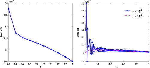
The approximate solution $v(x,t)$ and its absolute error at the final time T = 1 with N = 32, $n_s=5$ and $\tau =5\times {10}^{-3}$ are shown in Figure 1. Graphs of the absolute error $p\left(t\right)$ with different values of τ are illustrated in Figure 2 with N = 32, $n_s=5$ and $\tau =5\times {10}^{-3}$.

Figure 1. Graphs of approximate solution $v(x,1)$ (left plot) and its absolute error (right plot) with N = 32, $n_s=5$ and $\tau =5\times {10}^{-3}$ for Example 1.

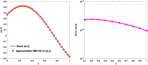
Figure 2. Graphs of the absolute error $p\left(t\right)$ with N = 32, $n_s=5$ and $\tau =5\times {10}^{-3}$ (right plot) and several values of τ (left plot) for Example 1.

6.2. Example 2

In Example 2, the 2-D case of Equations (1(1) $v_t(\mathbf{\text{x}},t)=\mathrm{\Delta }v(\mathbf{x},t)+p\left(t\right)v(\mathbf{x},t)+\varphi (\mathbf{x},t),(\mathbf{x},t)\in \mathrm{\Omega }\times (0,T],$(1) )–(3(3) $\begin{array}{rl}v(\mathbf{x},t)& =g(\mathbf{x},t),(\mathbf{x},t)\in \mathrm{\partial }\mathrm{\Omega }\times (0,T],\end{array}$(3) ) is considered on $\mathrm{\Omega }=[0,1{]}^2$ with [9,28,49] $\begin{array}{rl}\varphi (x,y,t)& =\left({\pi }^2-{(t+1)}^2\right)\exp (-t^2)\left(\cos \left(\pi x\right)+\sin \left(\pi y\right)\right),\\ g(0,y,t)& =\exp (-t^2)(\sin (\pi y)+1),g(1,y,t)=\exp (-t^2)(\sin (\pi y)-1),\\ g(x,0,t)& =\exp (-t^2)(\cos (\pi x\left)\right),g(x,1,t)=\exp (-t^2)(\cos (\pi x\left)\right),\\ f(x,y)& =\cos \left(\pi x\right)+\sin \left(\pi y\right),E\left(t\right)=\exp (-t^2)(\cos (\pi x^{\ast })+\sin (\pi y^{\ast }\left)\right),\end{array}$subject to the temperature overspecification condition at point ${\mathbf{x}}^{\mathbf{\ast }}=(x^{\ast },y^{\ast })=(0.2,0.2)$. The exact solutions are [49] $v(x,y,t)=\exp (-t^2)\left(\cos \left(\pi x\right)+\sin \left(\pi y\right)\right)\mathrm{a}\mathrm{n}\mathrm{d}p\left(t\right)=1+t^2.$We intend to solve this model by the RBF-FD method with various values of N, τ and T. Then, we compare the numerical results obtained with the results given in [22, 49].

Graphs of the numerical solutions $p\left(t\right)$ and $v(x,y,1)$ with N = 32, $n_s=5$ and $\tau ={10}^{-4}$ are shown in Figure 3. Moreover, the graphs and contours of the absolute error for $v(x,y,1)$ are plotted in this figure.

Figure 3. Graphs of numerical solution and absolute error for $v(x,1)$ and $p\left(t\right)$ for Example 2.

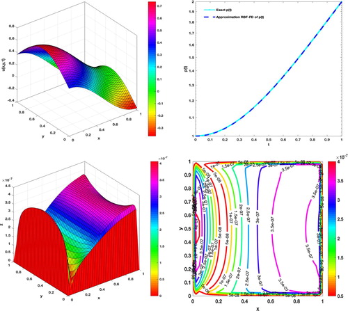
Table 6 presents the $E_2$ and $E_{\mathrm{\infty }}$ error norms and CPU time used by applying the RBF-FD method at different values of the final time by considering N = 20, 40 and $\tau =2.5\times {10}^{-3}$. Table 7 reports the absolute error in calculating $p\left(t\right)$ with $\tau =2.5\times {10}^{-3}$. Table 8 represents the maximum error in calculating $p\left(t\right)$ and $v(x,y,t)$ for several positions of ${\mathbf{x}}^{\mathbf{\ast }}$. This table implies that the RBF-FD method has the ability to approximate the solutions for different coordinates of ${\mathbf{x}}^{\mathbf{\ast }}$.

Table 6. The error obtained in approximating $v(x,y,t)$ by RBF-FD approach with $\tau =2.5\times {10}^{-3}$ and $n_s=5$ for Example 2.

		$N=20$		N = 40
t	$E_2$	$E_{\mathrm{\infty }}$	CPU time	$E_2$	$E_{\mathrm{\infty }}$	CPU time
0.1	$1.6130\times {10}^{-4}$	$1.6941\times {10}^{-5}$	0.15	$2.7418\times {10}^{-5}$	$1.0823\times {10}^{-6}$	3.08
0.2	$1.5853\times {10}^{-4}$	$1.6528\times {10}^{-5}$	0.33	$2.7581\times {10}^{-5}$	$1.0524\times {10}^{-6}$	$6.08$
0.3	$1.5138\times {10}^{-4}$	$1.5751\times {10}^{-5}$	0.51	$2.6427\times {10}^{-5}$	$1.0019\times {10}^{-6}$	10.10
0.4	$1.4165\times {10}^{-4}$	$1.4713\times {10}^{-5}$	0.67	$2.4796\times {10}^{-5}$	$9.3482\times {10}^{-7}$	13.43
0.5	$1.2997\times {10}^{-4}$	$1.3473\times {10}^{-5}$	0.83	$2.2816\times {10}^{-5}$	$8.5504\times {10}^{-7}$	$16.78$
0.6	$1.1693\times {10}^{-4}$	$1.2096\times {10}^{-5}$	0.94	$2.0590\times {10}^{-5}$	$7.6664\times {10}^{-7}$	20.31
0.7	$1.0314\times {10}^{-4}$	$1.0645\times {10}^{-5}$	1.11	$1.8224\times {10}^{-5}$	$6.7381\times {10}^{-7}$	23.59
0.8	$8.9214\times {10}^{-5}$	$9.1851\times {10}^{-6}$	1.38	$1.5822\times {10}^{-5}$	$5.8053\times {10}^{-7}$	26.90
0.9	$7.5666\times {10}^{-5}$	$7.7695\times {10}^{-6}$	$1.40$	$1.3472\times {10}^{-5}$	$4.9030\times {10}^{-7}$	$30.39$
1	$6.2929\times {10}^{-5}$	$6.4439\times {10}^{-6}$	$1.48$	$1.1253\times {10}^{-5}$	$4.0592\times {10}^{-7}$	33.65

Table 7. Comparison of the errors obtained in approximating $p\left(t\right)$ by RBF-FD approach and method of [22] for Example 2.

		RBF method [22]	RBF-FD method
t	Exact p	$N=15,\tau =2.5\times {10}^{-3}$	$N=20,n_s=3,\tau =2.5\times {10}^{-3}$
0.1	1.0100	$6.2108\times {10}^{-3}$	$1.4549\times {10}^{-4}$
0.2	1.0400	$5.6345\times {10}^{-3}$	$1.4832\times {10}^{-4}$
0.3	1.0900	$4.8933\times {10}^{-3}$	$1.4863\times {10}^{-4}$
0.4	1.1600	$3.8984\times {10}^{-3}$	$1.4882\times {10}^{-4}$
0.5	1.2500	$2.6064\times {10}^{-3}$	$1.4902\times {10}^{-4}$
0.6	1.3600	$9.7274\times {10}^{-4}$	$1.4925\times {10}^{-4}$
0.7	1.4900	$-1.0500\times {10}^{-3}$	$1.4950\times {10}^{-4}$
0.8	1.6400	$-3.5125\times {10}^{-3}$	$1.4978\times {10}^{-4}$
0.9	1.8100	$-6.4688\times {10}^{-3}$	$1.5008\times {10}^{-4}$
1	2.0000	$-4.8876\times {10}^{-3}$	$1.5042\times {10}^{-4}$

Table 8. The errors obtained in approximating $p\left(t\right)$ and $v(x,y,t)$ with N = 30, $\tau =5\times {10}^{-3}$ and several coordinates of ${\mathbf{x}}^{\mathbf{\ast }}$ for Example 2.

	${\mathbf{x}}^{\mathbf{\ast }}=(0.3,0.3)$		${\mathbf{x}}^{\mathbf{\ast }}=(0.5,0.5)$		${\mathbf{x}}^{\mathbf{\ast }}=(0.7,0.7)$
t	$p\left(t\right)$	$E_{\mathrm{\infty }}$	$p\left(t\right)$	$E_{\mathrm{\infty }}$	$p\left(t\right)$	$E_{\mathrm{\infty }}$
0.1	$2.3946\times {10}^{-5}$	$6.5436\times {10}^{-6}$	$1.5417\times {10}^{-5}$	$6.5395\times {10}^{-6}$	$7.0389\times {10}^{-5}$	$6.5658\times {10}^{-6}$
0.2	$2.4026\times {10}^{-5}$	$6.3574\times {10}^{-6}$	$1.5587\times {10}^{-5}$	$6.3529\times {10}^{-6}$	$5.9222\times {10}^{-5}$	$6.3762\times {10}^{-6}$
0.3	$2.4126\times {10}^{-5}$	$6.0534\times {10}^{-6}$	$1.5778\times {10}^{-5}$	$6.0495\times {10}^{-6}$	$5.8927\times {10}^{-5}$	$6.0697\times {10}^{-6}$
0.4	$2.4235\times {10}^{-5}$	$5.0503\times {10}^{-6}$	$1.5986\times {10}^{-5}$	$5.6470\times {10}^{-6}$	$5.8634\times {10}^{-5}$	$5.6639\times {10}^{-6}$
0.5	$2.4353\times {10}^{-5}$	$5.1700\times {10}^{-6}$	$1.6211\times {10}^{-5}$	$5.1674\times {10}^{-6}$	$5.8315\times {10}^{-5}$	$5.1808\times {10}^{-6}$
0.6	$2.4481\times {10}^{-5}$	$4.6372\times {10}^{-6}$	$1.6554\times {10}^{-5}$	$4.6353\times {10}^{-6}$	$5.7971\times {10}^{-5}$	$4.6454\times {10}^{-6}$
0.7	$2.4617\times {10}^{-5}$	$4.0774\times {10}^{-6}$	$1.6715\times {10}^{-5}$	$4.0760\times {10}^{-6}$	$5.7600\times {10}^{-5}$	$4.0831\times {10}^{-6}$
0.8	$2.4762\times {10}^{-5}$	$3.5145\times {10}^{-6}$	$1.6995\times {10}^{-5}$	$3.5136\times {10}^{-6}$	$5.7202\times {10}^{-5}$	$3.5180\times {10}^{-6}$
0.9	$2.4917\times {10}^{-5}$	$2.9696\times {10}^{-6}$	$1.7294\times {10}^{-5}$	$2.9692\times {10}^{-6}$	$5.6775\times {10}^{-5}$	$2.9713\times {10}^{-6}$
1	$2.5081\times {10}^{-5}$	$2.4597\times {10}^{-6}$	$1.7612\times {10}^{-5}$	$2.4596\times {10}^{-6}$	$5.6320\times {10}^{-5}$	$2.4600\times {10}^{-6}$

6.3. Example 3

In Example 3, the 2-D case of problem (1(1) $v_t(\mathbf{\text{x}},t)=\mathrm{\Delta }v(\mathbf{x},t)+p\left(t\right)v(\mathbf{x},t)+\varphi (\mathbf{x},t),(\mathbf{x},t)\in \mathrm{\Omega }\times (0,T],$(1) )–(3(3) $\begin{array}{rl}v(\mathbf{x},t)& =g(\mathbf{x},t),(\mathbf{x},t)\in \mathrm{\partial }\mathrm{\Omega }\times (0,T],\end{array}$(3) ) is considered on $\mathrm{\Omega }=[0,1{]}^2$ with [9,23,28] $\begin{array}{rl}\varphi (x,y,t)& =\exp \left(t\right)\sin \left(\frac{\pi }{4}(x+2y)\right)\left(\exp \left(t\right)+\frac{5{\pi }^2-48}{16}\right),\\ g(0,y,t)& =\exp \left(t\right)\sin \left(\frac{\pi }{2}y\right),g(1,y,t)=\exp \left(t\right)\sin \left(\frac{\pi }{4}(1+2y)\right),\\ g(x,0,t)& =\exp \left(t\right)\sin \left(\frac{\pi }{4}x\right),g(x,1,t)=\exp \left(t\right)\sin \left(\frac{\pi }{4}(x+2)\right),\\ f(x,y)& =\sin \left(\frac{\pi }{4}(x+2y)\right),E\left(t\right)=\exp \left(t\right)\sin \left(\frac{\pi }{4}(x^{\ast }+2y^{\ast })\right),\end{array}$subject to the temperature overspecification condition at point ${\mathbf{x}}^{\mathbf{\ast }}=(x^{\ast },y^{\ast })=(0.4,0.1)$. 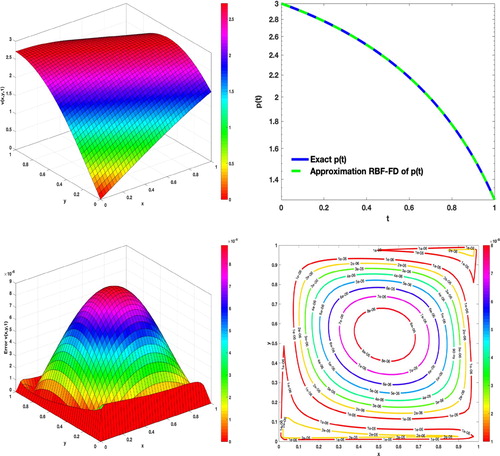The exact solutions are [23] $v(x,y,t)=\exp \left(t\right)\sin \left(\frac{\pi }{4}(x+2y)\right)\mathrm{a}\mathrm{n}\mathrm{d}p\left(t\right)=4-\exp \left(t\right).$Figure 4 shows the absolute errors in the calculation of $p\left(t\right)$ at various final times. Figure 5 depicts graphs of the numerical solutions $v(x,y,1)$ and $p\left(t\right)$ with $N=40,n_s=5$ and $\tau =5\times {10}^{-4}$. Graphs of the absolute error obtained with N = 40 and $5\times {10}^{-4}$ for $v(x,y,1)$ are presented in Figure 5.

Figure 4. Graph of the absolute error $p\left(t\right)$ with N = 40, $n_s=5$ and $\tau =5\times {10}^{-4}$ for Example 3.

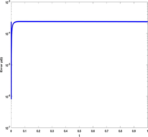
Figure 5. Graphs of the numerical solutions and absolute error with $N=40$ and $\tau =5\times {10}^{-4}$ for Example 3.

The $E_{\mathrm{\infty }}$ error norms and CPU time used by applying the RBF-FD method at different values of the final time by considering N = 20, 50 and $\tau ={10}^{-3}$ are reported in Table 9. Table 12 lists the absolute error of the solution $v(x,y,1)$ with $\tau ={10}^{-3}$ for different values of N. Tables 9 and 12 illustrate that the RBF-FD method is capable of approximating the solution $v(x,y,t)$ and parameter $p\left(t\right)$ with low computational time and acceptable accuracy. Tables 10 and 11 demonstrate that the RBF-FD method approximates the solutions accurately by considering the oversepcification condition at each point ${\mathbf{x}}^{\mathbf{\ast }}$ in the computational domain.

Table 9. The errors obtained in approximating $p\left(t\right)$ with $\tau ={10}^{-3}$ and $n_s=5$ for Example 3.

		N = 20		N = 50
t	Exact p	$E_{\mathrm{\infty }}$	CPU time	$E_{\mathrm{\infty }}$	CPU time
0.1	1.2817	$1.3161\times {10}^{-4}$	0.38	$1.1048\times {10}^{-4}$	28.91
0.2	2.7786	$1.3170\times {10}^{-4}$	0.87	$1.1043\times {10}^{-4}$	62.22
0.3	$2.6501$	$1.3179\times {10}^{-4}$	1.63	$1.1036\times {10}^{-4}$	89.70
0.4	2.5082	$1.3189\times {10}^{-4}$	1.80	$1.1029\times {10}^{-3}$	124.27
0.5	2.3513	$1.3200\times {10}^{-4}$	2.59	$1.1022\times {10}^{-3}$	158.81
0.6	2.1779	$1.3212\times {10}^{-4}$	3.40	$1.1013\times {10}^{-3}$	194.21
0.7	1.9862	$1.8805\times {10}^{-3}$	3.76	$1.9027\times {10}^{-3}$	231.65
0.8	1.7745	$1.3239\times {10}^{-4}$	3.57	$1.0994\times {10}^{-4}$	270.53
0.9	1.5404	$1.3255\times {10}^{-4}$	4.37	$1.0983\times {10}^{-4}$	313.27
1	$1.2817$	$1.3273\times {10}^{-4}$	4.40	$1.0907\times {10}^{-4}$	351.91

Table 10. The errors obtained in approximating $p\left(t\right)$ and $v(x,y,t)$ with N = 30, $\tau ={10}^{-2}$ and several coordinates of ${\mathbf{x}}^{\mathbf{\ast }}$ for Example 3.

	${\mathbf{x}}^{\mathbf{\ast }}=(0.3,0.4)$		${\mathbf{x}}^{\mathbf{\ast }}=(0.3,0.6)$		${\mathbf{x}}^{\mathbf{\ast }}=(0.3,0.8)$
t	$p\left(t\right)$	$E_{\mathrm{\infty }}$	$p\left(t\right)$	$E_{\mathrm{\infty }}$	$p\left(t\right)$	$E_{\mathrm{\infty }}$
0.1	$2.4057\times {10}^{-5}$	$8.2288\times {10}^{-6}$	$1.2019\times {10}^{-5}$	$8.0271\times {10}^{-6}$	$1.4409\times {10}^{-3}$	$6.4810\times {10}^{-6}$
0.2	$2.2626\times {10}^{-5}$	$9.1944\times {10}^{-6}$	$1.7778\times {10}^{-5}$	$8.9172\times {10}^{-6}$	$3.5244\times {10}^{-5}$	$7.5323\times {10}^{-6}$
0.3	$2.2714\times {10}^{-5}$	$1.0297\times {10}^{-5}$	$1.6078\times {10}^{-5}$	$9.9924\times {10}^{-6}$	$1.0831\times {10}^{-5}$	$8.3762\times {10}^{-6}$
0.4	$2.2840\times {10}^{-5}$	$1.1381\times {10}^{-5}$	$1.6203\times {10}^{-5}$	$1.1047\times {10}^{-5}$	$7.9218\times {10}^{-5}$	$9.2423\times {10}^{-6}$
0.5	$2.2960\times {10}^{-5}$	$1.2558\times {10}^{-5}$	$1.6463\times {10}^{-5}$	$1.2191\times {10}^{-6}$	$7.7780\times {10}^{-5}$	$1.0186\times {10}^{-5}$
0.6	$2.3090\times {10}^{-5}$	$1.3852\times {10}^{-5}$	$1.6606\times {10}^{-5}$	$1.3450\times {10}^{-5}$	$7.8214\times {10}^{-5}$	$1.1223\times {10}^{-5}$
0.7	$2.3232\times {10}^{-5}$	$1.5277\times {10}^{-5}$	$1.6753\times {10}^{-5}$	$1.4836\times {10}^{-5}$	$7.8758\times {10}^{-5}$	$1.2361\times {10}^{-5}$
0.8	$2.3388\times {10}^{-5}$	$1.6845\times {10}^{-5}$	$1.6914\times {10}^{-5}$	$1.6362\times {10}^{-5}$	$7.9358\times {10}^{-5}$	$1.3609\times {10}^{-5}$
0.9	$2.3557\times {10}^{-5}$	$1.8570\times {10}^{-5}$	$1.7090\times {10}^{-5}$	$1.8042\times {10}^{-5}$	$8.0016\times {10}^{-5}$	$1.4979\times {10}^{-5}$
1	$2.3740\times {10}^{-5}$	$2.0467\times {10}^{-5}$	$1.7283\times {10}^{-5}$	$1.9890\times {10}^{-5}$	$8.0738\times {10}^{-5}$	$1.6480\times {10}^{-5}$

Table 11. The errors obtained in approximating $p\left(t\right)$ and $v(x,y,t)$ with N = 30, $\tau ={10}^{-2}$ and several coordinates of ${\mathbf{x}}^{\mathbf{\ast }}$ for Example 3.

	${\mathbf{x}}^{\mathbf{\ast }}=(0.4,0.2)$		${\mathbf{x}}^{\mathbf{\ast }}=(0.4,0.6)$		${\mathbf{x}}^{\mathbf{\ast }}=(0.4,0.8)$
t	$p\left(t\right)$	$E_{\mathrm{\infty }}$	$p\left(t\right)$	$E_{\mathrm{\infty }}$	$p\left(t\right)$	$E_{\mathrm{\infty }}$
0.1	$1.9262\times {10}^{-5}$	$8.4650\times {10}^{-6}$	$5.2457\times {10}^{-6}$	$7.8591\times {10}^{-6}$	$1.4461\times {10}^{-3}$	$6.3601\times {10}^{-6}$
0.2	$3.3679\times {10}^{-5}$	$9.5161\times {10}^{-6}$	$1.2247\times {10}^{-5}$	$8.6995\times {10}^{-6}$	$3.5212\times {10}^{-4}$	$7.4071\times {10}^{-6}$
0.3	$2.9192\times {10}^{-5}$	$1.0654\times {10}^{-5}$	$1.0584\times {10}^{-5}$	$9.7336\times {10}^{-6}$	$1.0693\times {10}^{-4}$	$8.2384\times {10}^{-6}$
0.4	$3.0333\times {10}^{-5}$	$1.1775\times {10}^{-5}$	$1.0671\times {10}^{-5}$	$1.0762\times {10}^{-5}$	$7.7753\times {10}^{-5}$	$9.0904\times {10}^{-6}$
0.5	$3.0649\times {10}^{-5}$	$1.2992\times {10}^{-5}$	$1.0912\times {10}^{-5}$	$1.1877\times {10}^{-5}$	$7.6302\times {10}^{-5}$	$1.0019\times {10}^{-5}$
0.6	$3.0835\times {10}^{-5}$	$1.4332\times {10}^{-5}$	$1.1039\times {10}^{-5}$	$1.3105\times {10}^{-5}$	$7.6724\times {10}^{-5}$	$1.1038\times {10}^{-5}$
0.7	$3.1030\times {10}^{-5}$	$1.5807\times {10}^{-5}$	$1.1167\times {10}^{-5}$	$1.4557\times {10}^{-5}$	$7.7257\times {10}^{-5}$	$1.2157\times {10}^{-5}$
0.8	$3.1243\times {10}^{-5}$	$1.7429\times {10}^{-5}$	$1.1308\times {10}^{-5}$	$1.5945\times {10}^{-5}$	$7.7843\times {10}^{-5}$	$1.3385\times {10}^{-5}$
0.9	$3.1475\times {10}^{-5}$	$1.9214\times {10}^{-5}$	$1.1463\times {10}^{-5}$	$1.7584\times {10}^{-5}$	$7.8488\times {10}^{-5}$	$1.4732\times {10}^{-5}$
1	$3.1727\times {10}^{-5}$	$2.1177\times {10}^{-5}$	$1.1632\times {10}^{-5}$	$1.9386\times {10}^{-5}$	$7.9194\times {10}^{-5}$	$1.6208\times {10}^{-5}$

Table 12. The errors obtained in approximating $v(x,y,1)$ with $\tau ={10}^{-3}$ for Example 3.

$x_i$	$y_i$	N = 20	N = 50
0.1	0.1	$1.0865\times {10}^{-6}$	$4.6457\times {10}^{-7}$
0.2	0.2	$1.4563\times {10}^{-6}$	$1.7637\times {10}^{-7}$
0.3	0.3	$1.8261\times {10}^{-6}$	$8.9481\times {10}^{-7}$
0.4	0.4	$2.0692\times {10}^{-6}$	$1.5434\times {10}^{-6}$
0.5	0.5	$2.2511\times {10}^{-6}$	$2.0004\times {10}^{-6}$
0.6	0.6	$2.3266\times {10}^{-6}$	$2.1800\times {10}^{-6}$
0.7	0.7	$2.3009\times {10}^{-6}$	$2.0483\times {10}^{-6}$
0.8	0.8	$2.3691\times {10}^{-6}$	$1.6355\times {10}^{-6}$
0.9	0.9	$2.2165\times {10}^{-6}$	$1.0465\times {10}^{-6}$

6.4. Example 4

We consider the first inverse problem (1(1) $v_t(\mathbf{\text{x}},t)=\mathrm{\Delta }v(\mathbf{x},t)+p\left(t\right)v(\mathbf{x},t)+\varphi (\mathbf{x},t),(\mathbf{x},t)\in \mathrm{\Omega }\times (0,T],$(1) )–(3(3) $\begin{array}{rl}v(\mathbf{x},t)& =g(\mathbf{x},t),(\mathbf{x},t)\in \mathrm{\partial }\mathrm{\Omega }\times (0,T],\end{array}$(3) ) in the region $[0,1{]}^2$ with the exact solutions [23] $v(x,y,t)=\frac{(t^2+1)}{2}\log \left({(x-2)}^2+{(y-2)}^2\right)\mathrm{a}\mathrm{n}\mathrm{d}p\left(t\right)=\frac{1}{t+1}.$The initial and boundary conditions are extracted directly from the exact solution. Moreover, the function $E\left(t\right)$ is obtained by substituting the point ${\mathbf{x}}^{\ast }=(x^{\ast },y^{\ast })=(0.1,0.2)$ in the exact solution $E\left(t\right)=\frac{(t^2+1)}{2}\log \left({(x^{\ast }-2)}^2+{(y^{\ast }-2)}^2\right).$Figure 6 illustrates the graphs of the absolute errors for v and p at the final time T = 1 with N = 50, $n_s=5$ and $\tau ={10}^{-3}$. 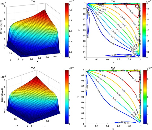Table 13 lists the errors of $v(x,y,t)$ and $p\left(t\right)$ and the CPU time used by employing the RBF-FD method at T = 2, 4. Graphs and contours of the absolute errors for $v(x,y,t)$ at final times T = 1, 5 are plotted in Figure 7.

Figure 6. Graphs of numerical solution $v(x,y,1)$ and $p\left(t\right)$ and their absolute errors with N = 50 and $\tau ={10}^{-3}$ for Example 4.

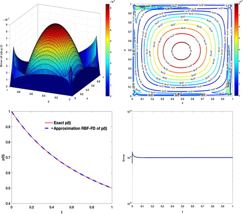
Table 13. The error obtained in approximating $v(x,y,t)$ and $p\left(t\right)$ with $\tau =\times {10}^{-3}$ and $n_s=5$ for Example 4.

	T = 2			T = 4
N	Error v(x,y,t)	Error p(t)	CPU time	Error v(x,y,t)	Error p(t)	CPU time
20	$1.5853\times {10}^{-4}$	$1.6528\times {10}^{-5}$	0.33	$2.7581\times {10}^{-5}$	$1.0524\times {10}^{-6}$	$6.08$
30	$1.5138\times {10}^{-4}$	$1.5751\times {10}^{-5}$	0.51	$2.6427\times {10}^{-5}$	$1.0019\times {10}^{-6}$	10.10
40	$1.2840\times {10}^{-6}$	$1.9018\times {10}^{-4}$	147.52	$4.3683\times {10}^{-6}$	$1.9016\times {10}^{-4}$	305.49

Figure 7. Graph and contour of the absolute errors $v(x,y,t)$ at different final times with N = 40 and $\tau ={10}^{-3}$ for Example 4.

6.5. Example 5

Now, we focus on the 3-D inverse problem (1(1) $v_t(\mathbf{\text{x}},t)=\mathrm{\Delta }v(\mathbf{x},t)+p\left(t\right)v(\mathbf{x},t)+\varphi (\mathbf{x},t),(\mathbf{x},t)\in \mathrm{\Omega }\times (0,T],$(1) )–(3(3) $\begin{array}{rl}v(\mathbf{x},t)& =g(\mathbf{x},t),(\mathbf{x},t)\in \mathrm{\partial }\mathrm{\Omega }\times (0,T],\end{array}$(3) ) with [24] $\varphi (x,y,z,t)=\left(\frac{7{\pi }^2}{8}-10t\right)\exp \left(t\right)\sin \left(\frac{\pi }{4}(x+2y+3z)\right)\mathrm{a}\mathrm{n}\mathrm{d}E\left(t\right)=\exp \left(t\right),$in which the temperature overspecification is defined at the point ${\mathbf{x}}^{\ast }=(x^{\ast },y^{\ast },z^{\ast })=(0.6,0.4,0.2).$ The initial and boundary conditions are obtained from the following exact solutions [24] $v(x,y,z,t)=\exp \left(t\right)\sin \left(\frac{\pi }{4}(x+2y+3z)\right)\mathrm{a}\mathrm{n}\mathrm{d}p\left(t\right)=1+10t.$Figs. 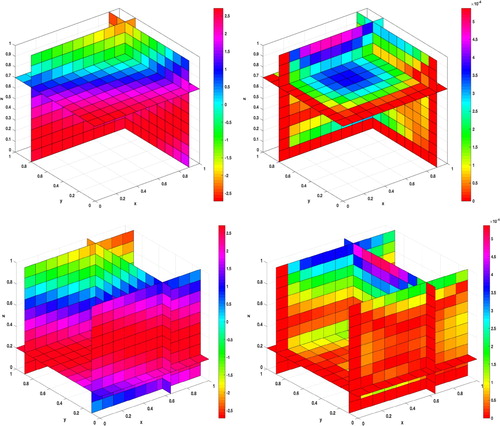8 depicts the numerical solutions and the absolute errors obtained by the RBF-FD method for $v(x,y,z,t)$ with N = 10, $n_s=3$ and $\tau ={10}^{-4}$.Table 14 reports the absolute error obtained in the calculation of $p\left(t\right)$ with $N=10,n_s=5$ and $\tau =5\times {10}^{-3}$. The absolute errors obtained by applying the RBF-FD method for calculating $v(x,y,z,T)$ with N = 10 and $\tau ={10}^{-3}$ at the final time T = 1 are shown in Table 15. Clearly, this method with fewer points N and a smaller time step τ has a similar accuracy with the method introduced in [24].

Figure 8. Graphs of the numerical and exact solution for $v(x,y,z,1)$ and its absolute error with N = 10, $n_s=3$ and $\tau ={10}^{-4}$ for Example 5.

6.6. Example 6

The 1-D inverse problem (1(1) $v_t(\mathbf{\text{x}},t)=\mathrm{\Delta }v(\mathbf{x},t)+p\left(t\right)v(\mathbf{x},t)+\varphi (\mathbf{x},t),(\mathbf{x},t)\in \mathrm{\Omega }\times (0,T],$(1) )–(3(3) $\begin{array}{rl}v(\mathbf{x},t)& =g(\mathbf{x},t),(\mathbf{x},t)\in \mathrm{\partial }\mathrm{\Omega }\times (0,T],\end{array}$(3) ) with the integral overspecification condition (5(5) ${\int }_{\mathrm{\Omega }}k\left(\mathbf{\text{x}}\right)v(\mathbf{\text{x}},t)\mathrm{d}\mathbf{\text{x}}=E\left(t\right),t\in [0,T],$(5) ) is presumed to have the following parameters $\begin{array}{rl}\varphi (x,t)& =\exp \left(t\right)\left[x+\cos \left(\pi x\right)+{\pi }^2\cos \left(\pi x\right)-(1+t^2)[x+\cos (\pi x\left)\right]\right],\\ E\left(t\right)& =\exp \left(t\right)\left(\frac{3}{4}-\frac{2}{{\pi }^2}\right),k\left(x\right)=1+x^2,\end{array}$for which the exact solutions are [46] $v(x,t)=\exp \left(t\right)\left[x+\cos \left(\pi x\right)\right]\mathrm{a}\mathrm{n}\mathrm{d}p\left(t\right)=1+t^2.$The exact solution is used to obtain the initial and boundary conditions for this sample.

Table 14. Comparison of the maximum error obtained in approximating $p\left(t\right)$ by the RBF-FD approach and the method of [24] for Example 5.

		7-point scheme [24]	RBF-FD method
		$N=50,\tau =6.6667\times {10}^{-5}$	$N=10,n_s=5,\tau =5\times {10}^{-3}$
t	Exact p	Error	absolute Error	RMS error	CPU time
0.1	$2.0000$	$8.8\times {10}^{-4}$	$1.8765\times {10}^{-3}$	$2.9685\times {10}^{-6}$	1.02
$0.2$	$3.0000$	$8.7\times {10}^{-4}$	$1.9025\times {10}^{-3}$	$3.2708\times {10}^{-6}$	2.04
$0.3$	4.0000	$8.8\times {10}^{-4}$	$1.9149\times {10}^{-3}$	$3.3932\times {10}^{-6}$	3.13
0.4	$5.0000$	$8.6\times {10}^{-4}$	$1.9282\times {10}^{-3}$	$3.4673\times {10}^{-6}$	4.23
0.5	6.0000	$8.5\times {10}^{-4}$	$1.9589\times {10}^{-3}$	$3.5228\times {10}^{-6}$	5.12
$0.6$	7.0000	$8.6\times {10}^{-4}$	$2.4666\times {10}^{-3}$	$3.5968\times {10}^{-6}$	5.85
$0.7$	8.0000	$8.6\times {10}^{-4}$	$1.9765\times {10}^{-3}$	$3.6128\times {10}^{-6}$	7.19
$0.8$	$9.0000$	$8.4\times {10}^{-4}$	$1.9959\times {10}^{-3}$	$3.6542\times {10}^{-6}$	7.86
$0.9$	10.0000	$8.3\times {10}^{-4}$	$2.0171\times {10}^{-3}$	$3.6955\times {10}^{-6}$	9.02
$1.0$	11.0000	$8.6\times {10}^{-4}$	$2.0405\times {10}^{-3}$	$3.7375\times {10}^{-6}$	10.26

Table 15. Comparison of the maximum error obtained in approximating $v(x,y,z,1)$ by the RBF-FD approach and the method of [24] for Example 5.

			7-point scheme [24]	RBF-FD method
$x_i$	$y_i$	$z_i$	$N=50,\tau =6.6667\times {10}^{-5}$	$N=10,n_s=5,\tau ={10}^{-3}$
0.1	0.1	$0.1$	$4.3\times {10}^{-4}$	$8.4035\times {10}^{-5}$
$0.2$	$0.2$	0.2	$4.7\times {10}^{-4}$	$6.6014\times {10}^{-5}$
$0.3$	$0.3$	0.3	$4.5\times {10}^{-4}$	$8.1390\times {10}^{-5}$
0.4	0.4	$0.4$	$4.8\times {10}^{-4}$	$1.3227\times {10}^{-4}$
$0.5$	0.5	$0.5$	$4.9\times {10}^{-4}$	$1.9550\times {10}^{-4}$
0.6	$0.6$	0.6	$4.9\times {10}^{-4}$	$2.4666\times {10}^{-4}$
$0.7$	$0.7$	0.7	$4.7\times {10}^{-4}$	$2.7146\times {10}^{-4}$
0.8	$0.8$	$0.8$	$4.6\times {10}^{-4}$	$2.7080\times {10}^{-4}$
$0.9$	$0.9$	0.9	$5.0\times {10}^{-4}$	$2.2088\times {10}^{-4}$

We are going to solve this model by the RBF-FD method and to compare the numerical results obtained with the results given in [46].

Table 16 demonstrates the absolute error acquired and the CPU time used by employing the RBF-FD method at the final time T = 1 considering N = 80 and $\tau ={10}^{-4}$. Moreover, Table 17 presents the absolute error obtained in computing $p\left(t\right)$. Table 16 reveals the fact that choosing a lower size of time step τ in this method leads to a more accurate solution than the method of [46]. From Table 17, it can be inferred that the parameter $p\left(t\right)$ is accurately calculated with low computational time.

Table 16. Comparison of the maximum error obtained in approximating $v(x,1)$ by the RBF-FD approach and the method of [46] for Example 6.

	$N=50,\tau =6.6667\times {10}^{-5}$			$N=80,\tau ={10}^{-4}$
$x_i$	Crank-Nicolson [46]	Saulyev I [46]	Saulyev II [46]	RBF-FD
0.1	$6.8\times {10}^{-3}$	$9.3\times {10}^{-3}$	$9.0\times {10}^{-3}$	$5.8831\times {10}^{-6}$
0.2	$6.9\times {10}^{-3}$	$9.5\times {10}^{-3}$	$9.9\times {10}^{-3}$	$4.0643\times {10}^{-6}$
0.3	$6.7\times {10}^{-3}$	$9.5\times {10}^{-3}$	$9.9\times {10}^{-8}$	$5.5737\times {10}^{-6}$
0.4	$6.5\times {10}^{-3}$	$9.9\times {10}^{-3}$	$9.8\times {10}^{-3}$	$1.9925\times {10}^{-5}$
0.5	$6.7\times {10}^{-3}$	$9.8\times {10}^{-3}$	$9.8\times {10}^{-3}$	$3.5347\times {10}^{-5}$
0.6	$6.7\times {10}^{-3}$	$9.8\times {10}^{-3}$	$9.9\times {10}^{-3}$	$4.7937\times {10}^{-5}$
0.7	$6.9\times {10}^{-3}$	$9.5\times {10}^{-3}$	$9.1\times {10}^{-3}$	$5.3828\times {10}^{-5}$
0.8	$6.3\times {10}^{-3}$	$9.8\times {10}^{-3}$	$9.0\times {10}^{-3}$	$4.9491\times {10}^{-5}$
0.9	$6.7\times {10}^{-3}$	$9.8\times {10}^{-3}$	$9.4\times {10}^{-3}$	$3.2007\times {10}^{-5}$

Table 17. Comparison of the maximum error obtained in approximating $p\left(t\right)$ by the RBF-FD approach and the method of [46] for Example 6.

	$N=50,\tau =6.6667\times {10}^{-5}$			$N=80,n_s=5,\tau ={10}^{-4}$
t	Crank-Nicolson [46]	Saulyev I [46]	Saulyev II [46]	RBF-FD	CPU time
0.1	$7.4\times {10}^{-3}$	$9.8\times {10}^{-3}$	$9.9\times {10}^{-3}$	$2.1919\times {10}^{-5}$	$7.32$
0.2	$7.7\times {10}^{-3}$	$9.9\times {10}^{-3}$	$9.8\times {10}^{-3}$	$2.4224\times {10}^{-5}$	7.42
0.3	$7.6\times {10}^{-3}$	$9.8\times {10}^{-3}$	$1.1\times {10}^{-3}$	$2.6772\times {10}^{-5}$	$7.48$
0.4	$7.9\times {10}^{-3}$	$9.9\times {10}^{-5}$	$9.9\times {10}^{-3}$	$2.9588\times {10}^{-5}$	$7.46$
0.5	$7.7\times {10}^{-3}$	$9.7\times {10}^{-3}$	$9.8\times {10}^{-3}$	$3.2699\times {10}^{-5}$	7.48
0.6	$7.7\times {10}^{-3}$	$9.8\times {10}^{-3}$	$9.5\times {10}^{-3}$	$3.6138\times {10}^{-5}$	7.50
0.7	$7.6\times {10}^{-3}$	$9.5\times {10}^{-3}$	$9.4\times {10}^{-3}$	$3.9939\times {10}^{-5}$	7.49
0.8	$7.3\times {10}^{-3}$	$9.4\times {10}^{-3}$	$9.2\times {10}^{-3}$	$4.4139\times {10}^{-5}$	$7.50$
0.9	$7.3\times {10}^{-3}$	$9.3\times {10}^{-3}$	$9.1\times {10}^{-3}$	$4.8782\times {10}^{-5}$	$7.54$
1	$7.1\times {10}^{-3}$	$9.2\times {10}^{-3}$	$9.0\times {10}^{-3}$	$5.3912\times {10}^{-5}$	$7.63$

6.7. Example 7

In this sample, the inverse problem (1(1) $v_t(\mathbf{\text{x}},t)=\mathrm{\Delta }v(\mathbf{x},t)+p\left(t\right)v(\mathbf{x},t)+\varphi (\mathbf{x},t),(\mathbf{x},t)\in \mathrm{\Omega }\times (0,T],$(1) )-(3(3) $\begin{array}{rl}v(\mathbf{x},t)& =g(\mathbf{x},t),(\mathbf{x},t)\in \mathrm{\partial }\mathrm{\Omega }\times (0,T],\end{array}$(3) ) in 2-D and the integral overspecification (5(5) ${\int }_{\mathrm{\Omega }}k\left(\mathbf{\text{x}}\right)v(\mathbf{\text{x}},t)\mathrm{d}\mathbf{\text{x}}=E\left(t\right),t\in [0,T],$(5) ) is considered with [9] $\begin{array}{rl}\varphi (x,y,t)& =\left(\frac{5{\pi }^2}{16}-5t\right)\exp \left(t\right)\sin \left(\frac{\pi }{4}(x+2y)\right),\\ E\left(t\right)& =\frac{8}{{\pi }^2}\exp \left(t\right)\left(\sin \left(\frac{\pi }{4}\right)-\sin \left(\frac{3\pi }{4}\right)+\sin \left(\frac{\pi }{2}\right)\right).\end{array}$The initial and boundary conditions for this model are extracted from the following exact solutions $v(x,y,t)=\exp \left(t\right)\sin \left(\frac{\pi }{4}(x+2y)\right)\mathrm{a}\mathrm{n}\mathrm{d}p\left(t\right)=1+5t.$We are going to solve this model by the RBF-FD method and to compare the numerical results obtained with the results given in [9].

We illustrate the behavior of the absolute error of $p\left(t\right)$ at different values of T and τ in Figure 9. Figure 10 shows the absolute error graphs related to $v(x,y,t)$ with N = 40, $n_s=5$ and $\tau =3\times {10}^{-4}$. In addition, the numerical solutions for $v(x,y,t)$ and $p\left(t\right)$ at the final time T = 1 are plotted in Figure 10. Table 18 lists the absolute error obtained for $v(x,y,t)$ at the final time T = 1 from the RBF-FD method by taking N = 50 and $\tau ={10}^{-2}$. In Table 19 the results obtained by the RBF-FD method are compared to those presented in [9].

Figure 9. The absolute error graphs of $p\left(t\right)$ with N = 50 and $\tau ={10}^{-3}$ (left plot) and with several values of τ (right plot) for Example 7.

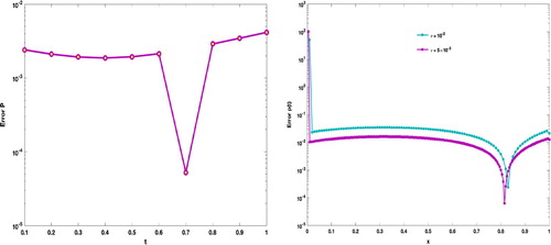
Figure 10. Graphs of the numerical solutions $v(x,y,1)$ and $p\left(t\right)$ and for Example 7.

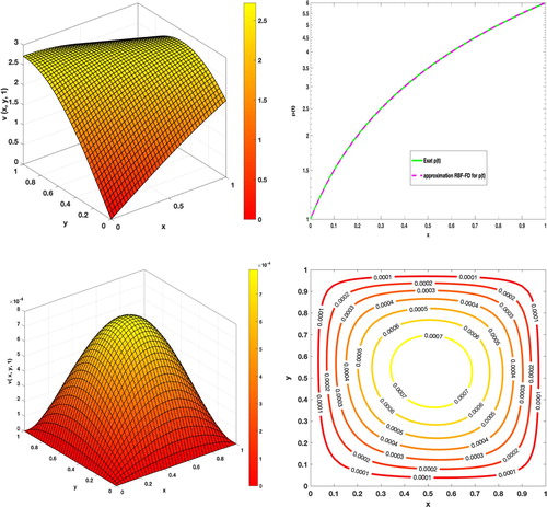
Table 18. Comparison of the maximum error obtained in approximating $v(x,y,1)$ by the RBF-FD approach and the method of [9] for Example 7.

		$N=50,\tau =6.6667\times {10}^{-5}$			$N=50,\tau ={10}^{-2}$
$x_i$	$y_i$	(5,1) Implicit [9]	Saulyev I [9]	Saulyev II [9]	RBF-FD
0.1	0.1	$7.0\times {10}^{-3}$	$5.1\times {10}^{-4}$	$5.0\times {10}^{-4}$	$5.0860\times {10}^{-5}$
0.2	0.2	$7.3\times {10}^{-3}$	$5.3\times {10}^{-4}$	$5.2\times {10}^{-4}$	$1.7434\times {10}^{-4}$
0.3	0.3	$7.5\times {10}^{-3}$	$5.2\times {10}^{-4}$	$5.1\times {10}^{-4}$	$3.1995\times {10}^{-4}$
0.4	0.4	$7.5\times {10}^{-3}$	$5.1\times {10}^{-4}$	$5.1\times {10}^{-4}$	$4.4076\times {10}^{-4}$
0.5	0.5	$7.6\times {10}^{-3}$	$5.0\times {10}^{-4}$	$5.3\times {10}^{-4}$	$5.0060\times {10}^{-4}$
0.6	0.6	$7.7\times {10}^{-3}$	$5.0\times {10}^{-4}$	$5.2\times {10}^{-4}$	$4.8073\times {10}^{-4}$
0.7	0.7	$7.4\times {10}^{-3}$	$5.3\times {10}^{-4}$	$5.1\times {10}^{-4}$	$3.8401\times {10}^{-4}$
0.8	0.8	$7.1\times {10}^{-3}$	$5.4\times {10}^{-4}$	$5.3\times {10}^{-4}$	$2.3580\times {10}^{-4}$
0.9	0.9	$6.8\times {10}^{-3}$	$5.2\times {10}^{-4}$	$5.3\times {10}^{-4}$	$8.3219\times {10}^{-5}$

Table 19. Comparison of the maximum error obtained in approximating $p\left(t\right)$ by the RBF-FD approach and the method of [9] for Example 7.

		$N=50,\tau =6.6667\times {10}^{-5}$			$N=40,\tau =5\times {10}^{-4}$
t	Exact p	(5,1) Implicit [9]	Saulyev I [9]	Saulyev II [9]	RBF-FD	CPU time
0.1	1.5000	$8.1\times {10}^{-3}$	$7.7\times {10}^{-3}$	$7.5\times {10}^{-3}$	$2.4074\times {10}^{-3}$	19.82
0.2	2.0000	$8.2\times {10}^{-3}$	$7.8\times {10}^{-3}$	$7.6\times {10}^{-3}$	$2.1030\times {10}^{-3}$	42.62
0.3	2.5000	$8.3\times {10}^{-3}$	$7.9\times {10}^{-4}$	$7.5\times {10}^{-3}$	$1.9234\times {10}^{-3}$	63.05
0.4	3.0000	$8.3\times {10}^{-3}$	$7.9\times {10}^{-3}$	$7.7\times {10}^{-3}$	$1.8683\times {10}^{-3}$	84.79
0.5	3.5000	$8.5\times {10}^{-3}$	$8.0\times {10}^{-3}$	$7.8\times {10}^{-3}$	$1.9376\times {10}^{-3}$	107.07
0.6	4.0000	$8.7\times {10}^{-3}$	$8.1\times {10}^{-3}$	$8.0\times {10}^{-3}$	$2.1314\times {10}^{-3}$	$132.74$
0.7	4.5000	$8.4\times {10}^{-3}$	$8.3\times {10}^{-3}$	$8.2\times {10}^{-3}$	$5.2282\times {10}^{-5}$	152.43
0.8	5.0000	$8.1\times {10}^{-3}$	$8.1\times {10}^{-3}$	$8.1\times {10}^{-3}$	$2.8923\times {10}^{-3}$	174.26
0.9	5.5000	$8.0\times {10}^{-3}$	$8.2\times {10}^{-3}$	$7.9\times {10}^{-3}$	$3.4594\times {10}^{-3}$	199.42
1	6.0000	$7.8\times {10}^{-3}$	$8.1\times {10}^{-3}$	$7.9\times {10}^{-3}$	$4.1509\times {10}^{-3}$	225.64

6.8. Example 8

We investigate the second inverse problem (20(20) $\begin{array}{rl}& u_t(\mathbf{\text{x}},t)=\mathrm{\Delta }u(\mathbf{\text{x}},t)+\frac{\varphi (\mathbf{\text{x}},t)}{E\left(t\right)}{\int }_{\mathrm{\Omega }}k\left(\mathbf{\text{x}}\right)u(\mathbf{\text{x}},t)\mathrm{d}\mathbf{\text{x}},(\mathbf{\text{x}},t)\in \mathrm{\Omega }\times [0,T],\end{array}$(20) )–(22(22) $\begin{array}{rl}& u(\mathbf{\text{x}},t)-\frac{g(\mathbf{\text{x}},t)}{E\left(t\right)}{\int }_{\mathrm{\Omega }}k\left(\mathbf{\text{x}}\right)u(\mathbf{\text{x}},t)\mathrm{d}\mathbf{\text{x}}=0,(\mathbf{\text{x}},t)\in \mathrm{\partial }\mathrm{\Omega }\times [0,T].\end{array}$(22) ) in the 3-D case on $\mathrm{\Omega }=[0,1{]}^3$ with [24] $\varphi (x,y,z,t)=\left(\frac{7{\pi }^2}{8}-10t\right)\exp \left(t\right)\sin \left(\frac{\pi }{4}(x+2y+3z)\right)\mathrm{a}\mathrm{n}\mathrm{d}E\left(t\right)=\frac{32\sqrt{2}}{3{\pi }^3}\exp \left(t\right),$whose the exact solutions are [24] (39) $v(x,y,z,t)=\exp \left(t\right)\sin \left(\frac{\pi }{4}(x+2y+3z)\right)\mathrm{a}\mathrm{n}\mathrm{d}p\left(t\right)=1+10t.$(39) Table 20 gives the results of approximating $v(x,y,z,t)$ in the final time T = 1 with different numbers of N and $n_s$. Figure 11 shows the numerical solutions and their errors for $v(x,y,z,1)$ with N = 20 and $\tau ={10}^{-4}$.

Figure 11. Graphs of the approximation solution $v(x,y,z,1)$ and its absolute error with N = 20, $n_s=5$ and $\tau ={10}^{-4}$ for Example 8.

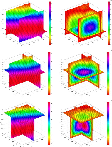
Table 20. The maximum error obtained in approximating $v(x,y,z,1)$ by the RBF-FD approach with $\tau ={10}^{-4}$ for Example 8.

			N = 10		N = 20
$x_i$	$y_i$	$z_i$	$n_s=3$	$n_s=5$	$n_s=3$	$n_s=5$
0.1	0.1	$0.1$	$2.9657\times {10}^{-3}$	$8.0101\times {10}^{-4}$	$7.3346\times {10}^{-4}$	$6.5053\times {10}^{-4}$
$0.2$	$0.2$	0.2	$1.3797\times {10}^{-2}$	$1.2552\times {10}^{-2}$	$3.3808\times {10}^{-3}$	$3.3583\times {10}^{-3}$
$0.3$	$0.3$	0.3	$2.7012\times {10}^{-2}$	$2.8083\times {10}^{-2}$	$6.9894\times {10}^{-3}$	$6.6618\times {10}^{-3}$
0.4	0.4	$0.4$	$3.4582\times {10}^{-2}$	$3.7311\times {10}^{-2}$	$8.4390\times {10}^{-3}$	$8.5517\times {10}^{-3}$
$0.5$	0.5	$0.5$	$3.1999\times {10}^{-2}$	$3.4748\times {10}^{-2}$	$7.7979\times {10}^{-3}$	$7.8019\times {10}^{-3}$
0.6	$0.6$	0.6	$2.0820\times {10}^{-2}$	$2.2266\times {10}^{-2}$	$5.0580\times {10}^{-3}$	$5.1005\times {10}^{-3}$
$0.7$	$0.7$	0.7	$7.4389\times {10}^{-3}$	$7.5490\times {10}^{-3}$	$1.7817\times {10}^{-3}$	$1.7623\times {10}^{-3}$
0.8	$0.8$	$0.8$	$1.0671\times {10}^{-3}$	$1.0286\times {10}^{-3}$	$3.0087\times {10}^{-4}$	$3.3695\times {10}^{-4}$
$0.9$	$0.9$	0.9	$1.9059\times {10}^{-3}$	$7.3584\times {10}^{-4}$	$5.0298\times {10}^{-4}$	$4.9587\times {10}^{-4}$

7. Conclusions

In this paper, the RBF-FD method was used to calculate the solution $v(x,t)$ and the control parameter $p\left(t\right)$ in two different inverse problems. Unlike the standard numerical procedures, the RBF-FD method operates without the need for mesh generation and by only using distributed points in the computational domain. Moreover, in this method, the values of the unknown function at the $n_s$ nearest points to each point are used to approximate the solution and its derivatives. By implementing this approach around all the domain points, the differentiation matrix is constructed by solving small linear systems. The most important advantage of this method is the production of sparse derivative matrices at a low computational cost. The parabolic inverse problems which are considered with either the temperature overspecification or energy overspecification conditions are solved by the RBF-FD method because of its low computational cost and easy implementation in high dimensions. The numerical results illustrate that this method is able to accurately calculate the solution $v(\mathbf{x},t)$ and the control parameter $p\left(t\right)$.

Acknowledgments

We would like to thank four referees for their valuable comments and helpful suggestions which have improved the paper.

Disclosure statement

No potential conflict of interest was reported by the author(s).

References

- Andrle M, Belgacem FB, El Badia A. Identification of moving pointwise sources in an advection–dispersion–reaction equation. Inverse Probl. 2011;27. doi:10.1088/0266-5611/27/2/025007.
- Andrle M, El Badia A. Identification of multiple moving pollution sources in surface waters or atmospheric media with boundary observations. Inverse Probl. 2012;28:075–009.
- Hamdi A. Detection and identification of multiple unknown time-dependent point sources occurring in 1D evolution transport equations. Inverse Probl Sci Eng. 2017;25(4):532–554.
- Hamdi A. Detection–identification of multiple unknown time–dependent point sources in a 2D transport equation: application to accidental pollution. Inverse Probl Sci Eng. 2017;25(10):1423–1447.
- Wang G, Li Y, Jiang M. Uniqueness theorems in bioluminescence tomography. Medical Phys. 2004;31:2289–2299.
- Abda AB, Hassen FB, Leblond J, et al. Sources recovery from boundary data: a model related to electroencephalography. Math Comput Model. 2009;49:2213–2223.
- Anastasio MA, Zhang J, Modgil D, et al. Application of inverse source concepts to photoacoustic tomography. Inverse Probl. 2007;23S21
- Cannon JR, Lin Y, Wang S. Determination of source parameter in parabolic equations. Meccanica. 1992;27:85–94.
- Dehghan M. Determination of a control parameter in the two–dimensional diffusion equation. Appl Numer Math. 2001;37:489–502.
- Deckert KL, Maple CG. Solution for diffusion equations with integral type boundary conditions. Proc Iowa Acad Sci. 1963;70:354–361.
- Lin Y. Analytical and numerical solutions for a class of non local nonlinear parabolic differential equations. J Math Anal. 1994;25:1577–1594.
- Macbain JA, Bednar JB. Existence and uniqueness properties for one-dimensional magnetotelluric inversion problem. J Math Phys. 1986;27:645–649.
- Prilepko AI, Soloev VV. Solvability of the inverse boundary value problem of finding a coefficient of a lower order term in a parabolic equation. Differ Equ. 1987;23:136–143.
- Rundell W, Colton DL. Determination of an unknown non–homogenous term in a linear partial differential equation from overspecified boundary data. Appl Anal. 1980;10:231–242.
- Dehghan M. Finding a control parameter in one–dimensional parabolic equations. Appl Math Comput. 2003;135:491–503.
- Dehghan M. Numerical solution of one–dimensional parabolic inverse problem. Appl Math Comput. 2003;136:333–344.
- Yousefi S, Dehghan M. Legendre multiscaling functions for solving the one–dimensional parabolic inverse problem. Numer Methods Partial Differ Equ. 2009;25:1502–1510.
- Dehghan M, Saadatmandi A. A tau method for the one–dimensional parabolic inverse problem subject to temperature overspecification. Comput Math Appl. 2006;52:933–940.
- Lakestani M, Dehghan M. The use of chebyshev cardinal functions for the solution of a partial differential equation with an unknown time–dependent coefficient subject to an extra measurement. J Comput Appl Math. 2010;235:669–678.
- Mohebbi A, Dehghan M. High–order scheme for determination of a control parameter in an inverse problem from the over–specified data. Comput Phys Commun. 2010;181:1947–1954.
- Dehghan M, Tatari M. Determination of a control parameter in a one–dimensional parabolic equation using the method of radial basis functions. Math Comput Model. 2006;44:1160–1168.
- Ma L, Wu Z. Radial basis functions method for parabolic inverse problem. Int J Comput Math. 2011;88:384–395.
- Takhtabnoos F, Shirzadi A. A greedy MLPG method for identifying a control parameter in 2D parabolic PDEs. Inverse Probl Sci Eng. 2018;26:1676–1694.
- Dehghan M. Determination of a control function in three–dimensional parabolic equations. Math Comput Simul. 2003;61:89–100.
- Dehghan M. An inverse problem of finding a source parameter in a semilinear parabolic equation. Appl Math Model. 2001;25:743–754.
- Dehghan M. Identifying a control function in two-dimensional parabolic inverse problems. Appl Math Comput. 2003;143:375–391.
- Wang S, Lin YP. A finite-difference solution to an inverse problem for determining a control function in a parabolic partial differential equation. Inverse Prob. 1989;5:631–640.
- Dehghan M. Fourth–order techniques for identifying a control parameter in the parabolic equations. Int J Eng Sci. 2002;40:433–447.
- Shamsi M, Dehghan M. Determination of a control function in three–dimensional parabolic equations by legendre pseudospectral method. Numer Methods Partial Differ Equ. 2012;28:74–93.
- Tolstykh AI. On using RBF–based differencing formulas for unstructured and mixed structured–unstructured grid calculations. In: Proceedings of the 16th IMACS World Congress, Vol. 228, Lausanne: IMACS; 2000. p. 4606–4624.
- Driscoll TA, Fornberg B. Interpolation in the limit of increasingly flat radial basis functions. Comput Math Appl. 2002;43:413–422.
- Wang JG, Liu GR. A point interpolation meshless method based on radial basis functions. Int J Numer Methods Eng. 2002;54:1623–1648.
- Shu C, Ding H, S.Yeo K. Local radial basis function=-based differential quadrature method and its application to solve two–dimensional incompressible navier–Stokes equations. Comput Methods Appl Mech Eng. 2003;192:941–954.
- Shu CW, Ding H, Zhao N, et al. Numerical comparison of least square-based finite- difference (LSFD) and radial basis function–based finite–difference (RBF-FD) methods. Comput Math Appl. 2006;51:1297–1310.
- Chandhini G, S. Sanyasiraju YVS. Local RBF-FD solutions for steady convection–diffusion problems. Internat J Numer Methods Eng. 2007;72:352–378.
- Flyer N, Lehto E, Blaise S, et al. A guide to RBF-generated finite differences for nonlinear transport: shallow water simulations on a sphere. J Comput Phys. 2012;231:4078–4095.
- Bolling EF, Flyer N, Erlebacher G. Solution to PDEs using radial basis function finite difference (RBF-FD) on multiple GPUs. J Comput Phys. 2012;231:7133–7151.
- Javed A, Djijdeli K, Xing JT. Shape adaptive RBF–FD implicit scheme for incompressible viscous Navier–Strokes equations. Comput Fluids. 2014;89:38–52.
- Dehghan M, Shafieeabyaneh NLocal radial basis function–finite–difference method to simulate some models in the nonlinear wave phenomena: regularized long–wave and extended fisher–Kolmogorov equations, Eng Comput. 2019. In press, doi:10.1007/s00366-019-00877-z.
- Fornberg B, Lehto E. Stabilization of RBF-generated finite difference methods for convective PDEs. J Comput Phys. 2011;230:2270–2285.
- Fornberg B. Calculation of weights in finite difference formulas. SIAM Rev. 1998;40:685–691.
- Wendland H. Scattered data approximation. England; Cambridge University Press; 2005. (Cambridge monograph on applied and computational mathematics).
- Fasshauer GE. Meshfree approximation methods with MATLAB. USA: World Scientific; 2007.
- Sarra SA. A local radial basis function method for advection–diffusion–reaction equations on complexly shaped domains. Appl Math Comput. 2012;218:9853–9865.
- Gerald CF. Applied numerical analysis. 4th Ed., Reading, MA: Addison-Wesley; 1989.
- Dehghan M. Parameter determination in a partial differential equation from the overspecified data. Math Comput Model. 2005;41:197–213.
- Dehghan M, Shakeri F. Method of lines solutions of the parabolic inverse problem with an overspecification at a point. Numer Algor. 2009;50:417–437.
- Cheng R. Determination of a control parameter in a one-dimensional parabolic equation using the moving least–square approximation. Int J Comput Math. 2008;85:1363–1373.
- Cheng R, Ge H. The meshless method for a two-dimensional parabolic problem with a source parameter. Appl Math Comput. 2008;202:730–737.