Nonlocal viscoelastic Euler-Bernoulli beam model: a Bayesian approach for parameter estimation using the delayed rejection adaptive metropolis algorithm

Abstract

The present work presents a model for nonlocal and viscoelastic Euler-Bernoulli beams and aspects of its calibration are addressed. The nonlocal feature of the model is described by the nonlocal elasticity theory proposed by Eringen and its viscoelastic behaviour is modelled by means of internal variables. Parametric analyses are performed to determine the impact of the nonlocal and viscoelastic parameters on the modal properties of the system. Inverse analyses are performed under the Bayesian framework and samples of the posterior density function are obtained by means of the Delayed Rejection Adaptive Metropolis (DRAM). The inverse analyses consider a nonlocal viscoelastic beam model with one internal variable and they address three aspects, namely: the impact of a misspecification of the beam diameter, the impact of modelling the beam diameter as an unknown but uninteresting model parameter and the model calibration when synthetic experimental data comes from a model containing two internal variables. The model parameters were chosen such that the system resembles a Single-Walled Carbon Nanotube (SWCNT).

Keywords:

• Nonlocal viscoelasticity
• internal variables
• parametric analysis
• Bayesian inference
• delayed rejection adaptive metropolis

2010 Mathematics Subject Classifications:

• 62F15
• 62D05
• 74Dxx

1. Introduction

Due to the superiority of their mechanical, electrical, thermal, chemical and optical properties, the carbon-based nanomaterials such as the Carbon Nanotubes (CNTs) and Graphene Sheets (GSs) are of great interest in science and technology and they find applications in nanoelectronics [1,2], nanosensors [3,4] and nanostructured composites [5,6]. However, since experimental analyses at the nanometre scale are extremely difficult to carry out, mathematical models for nanocomponents play an important role on the analysis and design of nanoelectromechanical systems.

Two approaches may be used to build models for nanostructures: atomistic modelling and continuum mechanics based modelling [7–9]. In the atomistic approach the structure is modelled considering the individual motion of each atom [10] and it has been reported to provide accurate predictions. On the other hand, the atomistic approach tends to be computationally prohibitive. Regarding the continuum mechanics approach, it is relatively simple and less computationally intense than the atomistic one. On the other hand, the classical (local) continuum elasticity theory fails on accurately modelling nanoscale structures due to the size dependence effects, which demands the use of nonlocal elasticity theories such as the one proposed by Eringen [11,12]. Mechanical models based on the nonlocal elasticity theory of Eringen have been proposed in the literature for modelling nanomaterials and nanoelectromechanical systems (NEMS) [13–23]. Inherent to these models is the nonlocal parameter $e_{0}a$, where $e_0$ is a material parameter and a is an internal characteristic length of the system, usually adopted as the length of the carbon-carbon bond. Although the nonlocal parameter is of fundamental importance in the theory of nonlocal elasticity, there is no consensus on its determination. As the experimental analyses at the nanometre scale are extremely difficult to carry out, most of these models are calibrated based on numerical results provided by atomistic approaches, specially from molecular dynamics simulations. Eringen [12] proposed for the material parameter the value $e_0=0.39$ by matching the dispersion curves of plane waves with those of Born-Karman model of atomic lattice dynamics and the value $e_0=0.31$ when considering the Rayleigh surface waves. Regarding the task of estimating the parameter $e_{0}a$, one finds works based on nonlocal Euler-Bernoulli beam model [24], nonlocal Timoshenko beam model [25] and nonlocal shell models [26–28]. The task of simultaneously estimating the nonlocal parameter $e_{0}a$ and Young's modulus of one dimensional atomic chains and armchair Single-Walled Carbon Nanotube SWCNTs is approached in [29].

Since the dynamic behaviour of a nanostructure may be significantly affected by damping or viscoelastic effects, an accurate modelling of these dissipative mechanisms is of prime importance [30–33]. At the nanoscale, the damping may be generated by external forces, such as magnetic forces [34], the interaction between the nanostructure and the substrate, humidity or thermal effects [35]. Regarding the description of dissipative mechanisms, generalized viscous and viscoelastic damping models are found in the literature within the context of nonlocal elasticity theory [36–39]. Nonlocality and viscoelastic models are approached, for instance, in the works by Lei [36,37], Ansari et al. [38] and Cajić et al. [39]. Nonlocal viscoelastic beam models embedded in viscoelastic mediums are addressed by Zhang et al. [40–42]. The aforementioned works on nonlocal viscoelastic damping models provide valuable insights about the dynamic behaviour of nanomaterials through parametric studies of the effects of nonlocal, viscoelastic and other parameters on their modal properties or time domain responses. However, it should be highlighted that none of them addresses the problem of estimating the nonlocal and/or viscoelastic parameters.

The present work is concerned with modelling nonlocal viscoelastic behaviour in Euler-Bernoulli beams and presenting aspects of the corresponding model calibration under the formalism of Bayesian inference [43]. The nonlocal model is described by the nonlocal elasticity theory proposed by Eringen [12] combined with the theory of internal variables for viscoelasticity [44–46]. The posterior probability density function (PDF) of the model parameters is sampled using the Delayed Rejection Adaptive Metropolis (DRAM) algorithm [47]. The inverse analyses consider a nonlocal viscoelastic beam model with one internal variable and they address three aspects, namely: the impact of a misspecification of the beam diameter, the impact of modelling the beam diameter as an unknown but uninteresting model parameter and the model calibration when synthetic experimental data comes from a model containing two internal variables. From the authors best knowledge, there exists no work in the literature that addresses the simultaneous estimation of the nonlocal parameter $e_{0}a$ and viscoelastic parameters using the Bayesian framework.

2. Mathematical modelling

2.1. Nonlocal elasticity theory

According to the nonlocal elasticity theory of Eringen [12], the stress $\mathit{\sigma }$ at a given reference point $\mathbf{x}$ in the body $\mathcal{B}$ depends on the strain field at every point ${\mathbf{x}}^{\prime }$ in the elastic domain. The nonlocal stress tensor $\mathit{\sigma }$ is given by (1) $\mathit{\sigma }(\mathbf{x})={\int }_{\mathcal{B}}K(|\mathbf{x}-{\mathbf{x}}^{\prime }|,\varphi )\mathit{\tau }({\mathbf{x}}^{\prime })\mathrm{d}{\mathbf{x}}^{\prime }$(1) where $\mathit{\tau }$ is the classical local stress tensor, the kernel function $K(|\mathbf{x}-{\mathbf{x}}^{\prime }|,\varphi )$ is the nonlocal modulus (attenuation function), $|\mathbf{x}-{\mathbf{x}}^{\prime }|$ is the Euclidean distance and ϕ is a material constant that depends on internal and external characteristic lengths, such as lattice distance and wave length, respectively. Usually, one has $\varphi =e_{0}a/l$, where $e_0$ is a parameter used for calibrating the nonlocal model by means of data obtained from experiments, a represents an internal characteristic length and l an external one.

The nonlocal kernel proposed by Eringen [12] is given by (2) $K(|\mathbf{z}|,\tau )=(2\pi l^2{\varphi }^2{)}^{-1}{\mathcal{K}}_{\mathbf{0}}\left(\frac{\sqrt{\mathbf{z}\cdot \mathbf{z}}}{l\varphi }\right)$(2) where ${\mathcal{K}}_{\mathbf{0}}$ is the modified Bessel function.

In order to obtain a differential form for the nonlocal constitutive relation in Equation (1(1) $\mathit{\sigma }(\mathbf{x})={\int }_{\mathcal{B}}K(|\mathbf{x}-{\mathbf{x}}^{\prime }|,\varphi )\mathit{\tau }({\mathbf{x}}^{\prime })\mathrm{d}{\mathbf{x}}^{\prime }$(1) ), the nonlocal kernel is considered as a Green's function of a linear differential operator as follows [12] (3) $\mathcal{L}[K(|\mathbf{x}-{\mathbf{x}}^{\prime }|,\varphi )]=\delta (|\mathbf{x}-{\mathbf{x}}^{\prime }|)$(3) where $\mathcal{L}(\bullet )$ is the linear differential operator and δ is the Dirac delta distribution. Applying the linear differential operator in the nonlocal constitutive relation in Equation (1(1) $\mathit{\sigma }(\mathbf{x})={\int }_{\mathcal{B}}K(|\mathbf{x}-{\mathbf{x}}^{\prime }|,\varphi )\mathit{\tau }({\mathbf{x}}^{\prime })\mathrm{d}{\mathbf{x}}^{\prime }$(1) ) and considering Equation (3(3) $\mathcal{L}[K(|\mathbf{x}-{\mathbf{x}}^{\prime }|,\varphi )]=\delta (|\mathbf{x}-{\mathbf{x}}^{\prime }|)$(3) ), one has (4) $\mathcal{L}[\mathit{\sigma }(\mathbf{x})]=\mathit{\tau }(\mathbf{x})$(4) Considering 1D apllications, one may combine Equation (4(4) $\mathcal{L}[\mathit{\sigma }(\mathbf{x})]=\mathit{\tau }(\mathbf{x})$(4) ) and the nonlocal modulus in Equation (2(2) $K(|\mathbf{z}|,\tau )=(2\pi l^2{\varphi }^2{)}^{-1}{\mathcal{K}}_{\mathbf{0}}\left(\frac{\sqrt{\mathbf{z}\cdot \mathbf{z}}}{l\varphi }\right)$(2) ) to obtain the nonlocal constitutive relation in differential form as follows (5) $(1-(e_{0}a{)}^2{\mathrm{\nabla }}^2)\sigma (\mathbf{x})=\tau (\mathbf{x})$(5) where ${\mathrm{\nabla }}^2$ is the Laplacian operator.

2.2. Nonlocal viscoelastic model based on internal variables

A nonlocal viscoelastic constitutive relation can be obtained by combining the nonlocal elasticity theory with a local constitutive viscoelastic relation [36]. For the one-dimensional case, the integral form of the local constitutive relation of a linear and homogeneous viscoelastic material is given by [48] (6) $\tau (x,t)={\int }_0^t{E}_{rel}(t-t^{\prime })\frac{\mathrm{\partial }\epsilon (x,t^{\prime })}{\mathrm{\partial }{t}^{\prime }}\mathrm{d}{t}^{\prime }$(6) where $E_{rel}$ is the extensional relaxation kernel of the viscoelastic material, τ and ε are, respectively, the longitudinal local stress and strain [49]. A one-dimensional nonlocal viscoelastic constitutive relation is provided by Equations (5(5) $(1-(e_{0}a{)}^2{\mathrm{\nabla }}^2)\sigma (\mathbf{x})=\tau (\mathbf{x})$(5) ) and (6(6) $\tau (x,t)={\int }_0^t{E}_{rel}(t-t^{\prime })\frac{\mathrm{\partial }\epsilon (x,t^{\prime })}{\mathrm{\partial }{t}^{\prime }}\mathrm{d}{t}^{\prime }$(6) ) as follows (7) $(1-(e_{0}a{)}^2\frac{{\mathrm{\partial }}^2}{\mathrm{\partial }{x}^2})\sigma (x,t)={\int }_0^t{E}_{rel}(t-t^{\prime })\frac{\mathrm{\partial }\epsilon (x,t^{\prime })}{\mathrm{\partial }{t}^{\prime }}\mathrm{d}{t}^{\prime }$(7) In the present work, the relaxation kernel is adopted as follows (8) $E_{rel}(t)=E_{\mathrm{\infty }}[1+\sum _{i=1}^N{\mathrm{\Delta }}_i{e}^{-{\mathrm{\Omega }}_{i}t}]$(8) where $E_{\mathrm{\infty }}$ is the relaxed or static modulus, N is the number of internal variables which in turn are in charge of describing viscoelastic dissipation mechanisms and ${\mathrm{\Delta }}_i$ and ${\mathrm{\Omega }}_i$ correspond to the the relaxation amplitude/modulus and to the inverse of relaxation time associated to the ith internal variable as shown next.

The combination of the Laplace transform of Equations (7(7) $(1-(e_{0}a{)}^2\frac{{\mathrm{\partial }}^2}{\mathrm{\partial }{x}^2})\sigma (x,t)={\int }_0^t{E}_{rel}(t-t^{\prime })\frac{\mathrm{\partial }\epsilon (x,t^{\prime })}{\mathrm{\partial }{t}^{\prime }}\mathrm{d}{t}^{\prime }$(7) ) and (8(8) $E_{rel}(t)=E_{\mathrm{\infty }}[1+\sum _{i=1}^N{\mathrm{\Delta }}_i{e}^{-{\mathrm{\Omega }}_{i}t}]$(8) ) leads to (9) $(1-(e_{0}a{)}^2\frac{{\mathrm{\partial }}^2}{\mathrm{\partial }{x}^2})\tilde{\sigma }(s)=E_{\mathrm{\infty }}[1+\sum _{i=1}^N\frac{s{\mathrm{\Delta }}_i}{s+{\mathrm{\Omega }}_i}]\tilde{\epsilon }(s)$(9) where $\tilde{q}(s)$ denotes the Laplace transform of the variable $q(t)$. The ith internal variable ${\tilde{\xi }}_i(s)$ is defined as follows (10) ${\tilde{\xi }}_i(s)=\left(\frac{{\mathrm{\Omega }}_i}{s+{\mathrm{\Omega }}_i}\right)\tilde{\epsilon }(s),i=1,\dots ,N$(10) Finally, combining Equations (9(9) $(1-(e_{0}a{)}^2\frac{{\mathrm{\partial }}^2}{\mathrm{\partial }{x}^2})\tilde{\sigma }(s)=E_{\mathrm{\infty }}[1+\sum _{i=1}^N\frac{s{\mathrm{\Delta }}_i}{s+{\mathrm{\Omega }}_i}]\tilde{\epsilon }(s)$(9) ) and (10(10) ${\tilde{\xi }}_i(s)=\left(\frac{{\mathrm{\Omega }}_i}{s+{\mathrm{\Omega }}_i}\right)\tilde{\epsilon }(s),i=1,\dots ,N$(10) ) and applying the inverse Laplace transform leads to the differential form of the constitutive relation of a nonlocal viscoelastic material (11) $\begin{array}{rl}(1-(e_{0}a{)}^2\frac{{\mathrm{\partial }}^2}{\mathrm{\partial }{x}^2})\sigma (t)& =E_{\mathrm{\infty }}\epsilon (t)+E_{\mathrm{\infty }}\sum _{i=1}^N{\mathrm{\Delta }}_i[\epsilon (t)-{\xi }_i(t)]\\ \frac{\mathrm{\partial }{\xi }_i(t)}{\mathrm{\partial }t}& ={\mathrm{\Omega }}_i[\epsilon (t)-{\xi }_i(t)]\end{array}$(11) where the second equation in (11(11) $\begin{array}{rl}(1-(e_{0}a{)}^2\frac{{\mathrm{\partial }}^2}{\mathrm{\partial }{x}^2})\sigma (t)& =E_{\mathrm{\infty }}\epsilon (t)+E_{\mathrm{\infty }}\sum _{i=1}^N{\mathrm{\Delta }}_i[\epsilon (t)-{\xi }_i(t)]\\ \frac{\mathrm{\partial }{\xi }_i(t)}{\mathrm{\partial }t}& ={\mathrm{\Omega }}_i[\epsilon (t)-{\xi }_i(t)]\end{array}$(11) ) is the evolution equation of the ith internal variable.

2.3. Nonlocal viscoelastic Euler-Bernoulli beam model

In the Euler-Bernoulli beam model [50], the resultant bending moment $M(x,t)$ is given by (12) $M(x,t)=-{\int }_A\sigma (x,z,t)z\mathrm{d}A$(12) where z is the coordinate along the thickness of the beam, such that the neutral plane is given by z = 0, $\sigma (x,z,t)$ is the axial stress and A is the cross sectional area.

The governing equation of the Euler-Bernoulli beam model casts as follows (13) $\frac{{\mathrm{\partial }}^{2}M(x,t)}{\mathrm{\partial }{x}^2}=\rho A\frac{{\mathrm{\partial }}^{2}w(x,t)}{\mathrm{\partial }{t}^2}+C\frac{\mathrm{\partial }w(x,t)}{\mathrm{\partial }t}-f(x,t)$(13) where ρ is the mass density, w is the transverse deflection of the midline of the beam, C is the viscous damping coefficient and f is the distributed transverse load per unit length.

Applying the nonlocal operator $(1-(e_{0}a{)}^2\frac{{\mathrm{\partial }}^2}{\mathrm{\partial }{x}^2})$ in Equation (12(12) $M(x,t)=-{\int }_A\sigma (x,z,t)z\mathrm{d}A$(12) ) and considering the first equation in Equation (11(11) $\begin{array}{rl}(1-(e_{0}a{)}^2\frac{{\mathrm{\partial }}^2}{\mathrm{\partial }{x}^2})\sigma (t)& =E_{\mathrm{\infty }}\epsilon (t)+E_{\mathrm{\infty }}\sum _{i=1}^N{\mathrm{\Delta }}_i[\epsilon (t)-{\xi }_i(t)]\\ \frac{\mathrm{\partial }{\xi }_i(t)}{\mathrm{\partial }t}& ={\mathrm{\Omega }}_i[\epsilon (t)-{\xi }_i(t)]\end{array}$(11) ) leads to (14) $\begin{array}{rl}(1-(e_{0}a{)}^2\frac{{\mathrm{\partial }}^2}{\mathrm{\partial }{x}^2})M(x,t)& ={\int }_A{E}_{\mathrm{\infty }}\epsilon (x,z,t)z\mathrm{d}A\\ & +{\int }_A{E}_{\mathrm{\infty }}\sum _{i=1}^N{\mathrm{\Delta }}_i[\epsilon (x,z,t)-{\xi }_i(x,z,t)]z\mathrm{d}A\end{array}$(14) Considering the kinematics description assumed for Euler-Bernoulli beams and the hypotheses of small strains and small displacements, the axial strain is given as (15) $\epsilon (x,z,t)=-z\frac{{\mathrm{\partial }}^{2}w(x,t)}{\mathrm{\partial }{x}^2}$(15) As for the internal variables ${\xi }_i(x,z,t)$, inspired by Equation (10(10) ${\tilde{\xi }}_i(s)=\left(\frac{{\mathrm{\Omega }}_i}{s+{\mathrm{\Omega }}_i}\right)\tilde{\epsilon }(s),i=1,\dots ,N$(10) ), one may consider its definition linked to an auxiliary internal field ${\overline{w}}_i(x,t)$ as follows (16) ${\xi }_i(x,z,t)=-z\frac{{\mathrm{\partial }}^2{\overline{w}}_i(x,t)}{\mathrm{\partial }{x}^2}$(16) where the governing equation for ${\xi }_i(x,z,t)$ is given as (17) $\frac{\mathrm{\partial }{\overline{w}}_i(x,t)}{\mathrm{\partial }t}={\mathrm{\Omega }}_i[w(x,t)-{\overline{w}}_i(x,t)],i=1,\dots ,N$(17) Substituting Equations (15(15) $\epsilon (x,z,t)=-z\frac{{\mathrm{\partial }}^{2}w(x,t)}{\mathrm{\partial }{x}^2}$(15) ) and (16(16) ${\xi }_i(x,z,t)=-z\frac{{\mathrm{\partial }}^2{\overline{w}}_i(x,t)}{\mathrm{\partial }{x}^2}$(16) ) into Equation (14(14) $\begin{array}{rl}(1-(e_{0}a{)}^2\frac{{\mathrm{\partial }}^2}{\mathrm{\partial }{x}^2})M(x,t)& ={\int }_A{E}_{\mathrm{\infty }}\epsilon (x,z,t)z\mathrm{d}A\\ & +{\int }_A{E}_{\mathrm{\infty }}\sum _{i=1}^N{\mathrm{\Delta }}_i[\epsilon (x,z,t)-{\xi }_i(x,z,t)]z\mathrm{d}A\end{array}$(14) ) leads to (18) $(1-(e_{0}a{)}^2\frac{{\mathrm{\partial }}^2}{\mathrm{\partial }{x}^2})M(x,t)=-E_{\mathrm{\infty }}I[\frac{{\mathrm{\partial }}^{2}w(x,t)}{\mathrm{\partial }{x}^2}-\sum _{i=1}^N{\mathrm{\Delta }}_i(\frac{{\mathrm{\partial }}^{2}w(x,t)}{\mathrm{\partial }{x}^2}-\frac{{\mathrm{\partial }}^2{\overline{w}}_i(x,t)}{\mathrm{\partial }{x}^2})]$(18) where I is the cross-sectional area moment of inertia about the y axis.

Considering Equations (13(13) $\frac{{\mathrm{\partial }}^{2}M(x,t)}{\mathrm{\partial }{x}^2}=\rho A\frac{{\mathrm{\partial }}^{2}w(x,t)}{\mathrm{\partial }{t}^2}+C\frac{\mathrm{\partial }w(x,t)}{\mathrm{\partial }t}-f(x,t)$(13) ), (17(17) $\frac{\mathrm{\partial }{\overline{w}}_i(x,t)}{\mathrm{\partial }t}={\mathrm{\Omega }}_i[w(x,t)-{\overline{w}}_i(x,t)],i=1,\dots ,N$(17) ) and (18(18) $(1-(e_{0}a{)}^2\frac{{\mathrm{\partial }}^2}{\mathrm{\partial }{x}^2})M(x,t)=-E_{\mathrm{\infty }}I[\frac{{\mathrm{\partial }}^{2}w(x,t)}{\mathrm{\partial }{x}^2}-\sum _{i=1}^N{\mathrm{\Delta }}_i(\frac{{\mathrm{\partial }}^{2}w(x,t)}{\mathrm{\partial }{x}^2}-\frac{{\mathrm{\partial }}^2{\overline{w}}_i(x,t)}{\mathrm{\partial }{x}^2})]$(18) ), the differential equations that govern the dynamics of the nonlocal viscoelastic Euler-Bernoulli beam cast as follows (19) $\begin{array}{rl}& (1-(e_{0}a{)}^2\frac{{\mathrm{\partial }}^2}{\mathrm{\partial }{x}^2})\rho A\frac{{\mathrm{\partial }}^{2}w(x,t)}{\mathrm{\partial }{t}^2}+(1-(e_{0}a{)}^2\frac{{\mathrm{\partial }}^2}{\mathrm{\partial }{x}^2})C\frac{\mathrm{\partial }w(x,t)}{\mathrm{\partial }t}+E_{\mathrm{\infty }}I\frac{{\mathrm{\partial }}^{4}w(x,t)}{\mathrm{\partial }{x}^4}\\ & +E_{\mathrm{\infty }}I\sum _{i=1}^N{\mathrm{\Delta }}_i(\frac{{\mathrm{\partial }}^{4}w(x,t)}{\mathrm{\partial }{x}^4}-\frac{{\mathrm{\partial }}^4{\overline{w}}_i(x,t)}{\mathrm{\partial }{x}^4})=(1-(e_{0}a{)}^2\frac{{\mathrm{\partial }}^2}{\mathrm{\partial }{x}^2})f(x,t)\\ & \frac{\mathrm{\partial }}{\mathrm{\partial }t}\left(\frac{{\mathrm{\partial }}^4{\overline{w}}_i(x,t)}{\mathrm{\partial }{x}^4}\right)={\mathrm{\Omega }}_i[\frac{{\mathrm{\partial }}^{4}w(x,t)}{\mathrm{\partial }{x}^4}-\frac{{\mathrm{\partial }}^4{\overline{w}}_i(x,t)}{\mathrm{\partial }{x}^4}],i=1,\dots ,N\end{array}$(19) Equation (19(19) $\begin{array}{rl}& (1-(e_{0}a{)}^2\frac{{\mathrm{\partial }}^2}{\mathrm{\partial }{x}^2})\rho A\frac{{\mathrm{\partial }}^{2}w(x,t)}{\mathrm{\partial }{t}^2}+(1-(e_{0}a{)}^2\frac{{\mathrm{\partial }}^2}{\mathrm{\partial }{x}^2})C\frac{\mathrm{\partial }w(x,t)}{\mathrm{\partial }t}+E_{\mathrm{\infty }}I\frac{{\mathrm{\partial }}^{4}w(x,t)}{\mathrm{\partial }{x}^4}\\ & +E_{\mathrm{\infty }}I\sum _{i=1}^N{\mathrm{\Delta }}_i(\frac{{\mathrm{\partial }}^{4}w(x,t)}{\mathrm{\partial }{x}^4}-\frac{{\mathrm{\partial }}^4{\overline{w}}_i(x,t)}{\mathrm{\partial }{x}^4})=(1-(e_{0}a{)}^2\frac{{\mathrm{\partial }}^2}{\mathrm{\partial }{x}^2})f(x,t)\\ & \frac{\mathrm{\partial }}{\mathrm{\partial }t}\left(\frac{{\mathrm{\partial }}^4{\overline{w}}_i(x,t)}{\mathrm{\partial }{x}^4}\right)={\mathrm{\Omega }}_i[\frac{{\mathrm{\partial }}^{4}w(x,t)}{\mathrm{\partial }{x}^4}-\frac{{\mathrm{\partial }}^4{\overline{w}}_i(x,t)}{\mathrm{\partial }{x}^4}],i=1,\dots ,N\end{array}$(19) ) is a generalization of the Euler-Bernoulli beam model. For instance, the equation of motion of a local and undamped Euler-Bernoulli beam may be obtained by taking $e_{0}a=0$, C = 0 and ${\mathrm{\Delta }}_i=0$ and the equation of an undamped nonlocal Euler-Bernoulli beam is obtained by taking C = 0 and ${\mathrm{\Delta }}_i=0$, $i=1,2,\dots ,N$.

2.4. Finite element model of a nonlocal and viscoelastic Euler-Bernoulli beam

In this work, the finite element model of the nonlocal viscoelastic Euler-Bernoulli beam is derived by means of the weighted residuals approach [19,51]. Starting from Equation (19(19) $\begin{array}{rl}& (1-(e_{0}a{)}^2\frac{{\mathrm{\partial }}^2}{\mathrm{\partial }{x}^2})\rho A\frac{{\mathrm{\partial }}^{2}w(x,t)}{\mathrm{\partial }{t}^2}+(1-(e_{0}a{)}^2\frac{{\mathrm{\partial }}^2}{\mathrm{\partial }{x}^2})C\frac{\mathrm{\partial }w(x,t)}{\mathrm{\partial }t}+E_{\mathrm{\infty }}I\frac{{\mathrm{\partial }}^{4}w(x,t)}{\mathrm{\partial }{x}^4}\\ & +E_{\mathrm{\infty }}I\sum _{i=1}^N{\mathrm{\Delta }}_i(\frac{{\mathrm{\partial }}^{4}w(x,t)}{\mathrm{\partial }{x}^4}-\frac{{\mathrm{\partial }}^4{\overline{w}}_i(x,t)}{\mathrm{\partial }{x}^4})=(1-(e_{0}a{)}^2\frac{{\mathrm{\partial }}^2}{\mathrm{\partial }{x}^2})f(x,t)\\ & \frac{\mathrm{\partial }}{\mathrm{\partial }t}\left(\frac{{\mathrm{\partial }}^4{\overline{w}}_i(x,t)}{\mathrm{\partial }{x}^4}\right)={\mathrm{\Omega }}_i[\frac{{\mathrm{\partial }}^{4}w(x,t)}{\mathrm{\partial }{x}^4}-\frac{{\mathrm{\partial }}^4{\overline{w}}_i(x,t)}{\mathrm{\partial }{x}^4}],i=1,\dots ,N\end{array}$(19) ), the weighted-integral equations within a finite element of the beam may be written as (20) $\begin{array}{rl}& {\int }_0^{l_e}[(1-(e_{0}a{)}^2\frac{{\mathrm{\partial }}^2}{\mathrm{\partial }{\overline{x}}^2})\rho A\frac{{\mathrm{\partial }}^{2}w}{\mathrm{\partial }{t}^2}+(1-(e_{0}a{)}^2\frac{{\mathrm{\partial }}^2}{\mathrm{\partial }{\overline{x}}^2})C\frac{\mathrm{\partial }w}{\mathrm{\partial }t}+E_{\mathrm{\infty }}I[1+\sum _{i=1}^N{\mathrm{\Delta }}_i]\frac{{\mathrm{\partial }}^{4}w}{\mathrm{\partial }{\overline{x}}^4}\\ & -E_{\mathrm{\infty }}I\sum _{i=1}^N{\mathrm{\Delta }}_i\frac{{\mathrm{\partial }}^4{\overline{w}}_i}{\mathrm{\partial }{\overline{x}}^4}-(1-(e_{0}a{)}^2\frac{{\mathrm{\partial }}^2}{\mathrm{\partial }{\overline{x}}^2})f]\chi \mathrm{d}\overline{x}=0\\ & {\int }_0^{l_e}[E_{\mathrm{\infty }}I\frac{{\mathrm{\partial }}^5{\overline{w}}_i}{\mathrm{\partial }t\mathrm{\partial }{\overline{x}}^4}-{\mathrm{\Omega }}_i{E}_{\mathrm{\infty }}I(\frac{{\mathrm{\partial }}^{4}w}{\mathrm{\partial }{\overline{x}}^4}-\frac{{\mathrm{\partial }}^4{\overline{w}}_i}{\mathrm{\partial }{\overline{x}}^4})]\chi \mathrm{d}\overline{x}=0,i=1,2,\dots ,N\end{array}$(20) where $l_e$ denotes the length of the element, $\overline{x}$ represents the local coordinate and $\chi (x)$ is the Galerkin's weight function [51].

Considering Hermite interpolation functions for the transverse displacement and for the corresponding auxiliary internal field, within a finite element of the beam, one has (21) $\begin{array}{rl}& w(\overline{x},t)={\mathbf{N}}^{\mathrm{T}}(\overline{x}){\mathbf{q}}_e(t)\\ & {\overline{w}}_i(\overline{x},t)={\mathbf{N}}^{\mathrm{T}}(\overline{x}){\overline{\mathbf{q}}}_{ei}(t),i=1,2,\dots ,N\end{array}$(21) where $\mathbf{N}(\overline{x})$ is the matrix comprised of the interpolation functions, ${\mathbf{q}}_e(t)$ is the vector of generalized nodal displacements of the element and ${\overline{\mathbf{q}}}_{ei}(t)$ is the vector describing the variables of ith internal variable.

The governing equations of a beam element is given as follows (22) $\begin{array}{rl}& {\mathbf{M}}_e{\ddot{\mathbf{q}}}_e(t)+{\mathbf{D}}_e{\dot{\mathbf{q}}}_e(t)+[1+\sum _{i=1}^N{\mathrm{\Delta }}_i]{\mathbf{K}}_e{\mathbf{q}}_e(t)-{\mathbf{K}}_e\sum _{i=1}^N{\mathrm{\Delta }}_i{\overline{\mathbf{q}}}_{ei}(t)={\mathbf{P}}_e(t)\\ & \frac{{\mathrm{\Delta }}_i}{{\mathrm{\Omega }}_i}{\mathbf{K}}_e{\dot{\overline{\mathbf{q}}}}_{ei}(t)+{\mathrm{\Delta }}_i{\mathbf{K}}_e{\overline{\mathbf{q}}}_{ei}(t)-{\mathrm{\Delta }}_i{\mathbf{K}}_e{\mathbf{q}}_e(t)=\mathbf{0},i=1,2,\dots ,N\end{array}$(22) where ${\mathbf{M}}_e$, ${\mathbf{D}}_e$ and ${\mathbf{K}}_e$ are, respectively, the mass, viscous damping and relaxed stiffness matrices of a finite element and ${\mathbf{P}}_e$ is the vector of generalized nodal forces. The assembly of element matrices allows one to build the finite element model of the nonlocal viscoelastic beam. Finally, the vectors and matrices in Equation (22(22) $\begin{array}{rl}& {\mathbf{M}}_e{\ddot{\mathbf{q}}}_e(t)+{\mathbf{D}}_e{\dot{\mathbf{q}}}_e(t)+[1+\sum _{i=1}^N{\mathrm{\Delta }}_i]{\mathbf{K}}_e{\mathbf{q}}_e(t)-{\mathbf{K}}_e\sum _{i=1}^N{\mathrm{\Delta }}_i{\overline{\mathbf{q}}}_{ei}(t)={\mathbf{P}}_e(t)\\ & \frac{{\mathrm{\Delta }}_i}{{\mathrm{\Omega }}_i}{\mathbf{K}}_e{\dot{\overline{\mathbf{q}}}}_{ei}(t)+{\mathrm{\Delta }}_i{\mathbf{K}}_e{\overline{\mathbf{q}}}_{ei}(t)-{\mathrm{\Delta }}_i{\mathbf{K}}_e{\mathbf{q}}_e(t)=\mathbf{0},i=1,2,\dots ,N\end{array}$(22) ) are defined in Appendix 1.

3. Inverse problem

In the Bayesian framework for inverse problems, model parameters $\mathit{\theta }\in {\mathbb{R}}^{N_{\theta }}$ are modelled as random variables, uncertainties associated to a random variable are described by means of its probability density function (PDF) and the problem solution becomes the determination of the posterior PDF of model parameters given a set of measured data ${\mathbf{y}}_E\in {\mathbb{R}}^{N_y}$ [43], namely $\pi (\mathit{\theta }|{\mathbf{y}}_E)$.

Assuming an additive error observation model one may write (23) ${\mathbf{y}}_E=\mathbf{A}(\mathit{\theta })+\mathit{ϵ}$(23) where $\mathit{ϵ}$ is a random vector in charge of representing measurement errors and $\mathbf{A}(\mathit{\theta }):{\mathbb{R}}^{N_{\theta }}\mapsto {\mathbb{R}}^{N_y}$ is an operator used to provide model predictions. As $\mathit{\theta }$, ${\mathbf{y}}_E$ and $\mathit{ϵ}$ are random variables, one may obtain a relation among them by means of the Bayes rule as follows (24) $\pi (\mathit{\theta }|{\mathbf{y}}_E)=\frac{\pi ({\mathbf{y}}_E|\mathit{\theta })\pi (\mathit{\theta })}{\pi ({\mathbf{y}}_E)}$(24) where $\pi (\mathit{\theta }|{\mathbf{y}}_E)$ is the posterior PDF of model parameters, $\pi ({\mathbf{y}}_E|\mathit{\theta })$ is the likelihood function and $\pi (\mathit{\theta })$ is the prior density, which in turn represents the information one has about the parameters before considering any information about the experimental data ${\mathbf{y}}_E$. Concerning $\pi ({\mathbf{y}}_E)$, it represents the distribution of measured data and is given by (25) $\pi ({\mathbf{y}}_E)=\int \pi ({\mathbf{y}}_E|\mathit{\theta })\pi (\mathit{\theta })\mathrm{d}\mathit{\theta }$(25) Assuming that $\mathit{ϵ}$ follows a zero mean Gaussian density with covariance matrix ${\mathbf{\Sigma }}_{ϵϵ}$ formally represented by $\mathit{ϵ}\sim \mathcal{N}(\mathbf{0},{\mathbf{\Sigma }}_{ϵϵ})$, and that $\mathit{ϵ}$ and $\mathit{\theta }$ are independent random variables, the likelihood function is given (26) $\pi ({\mathbf{y}}_E|\mathit{\theta })=\frac{1}{\sqrt{(2\pi {)}^{N_y}}\sqrt{det\left({\mathbf{\Sigma }}_{ϵϵ}\right)}}\exp [-\frac{1}{2}{({\mathbf{y}}_E-\mathbf{A}\mathbf{(}\mathit{\theta }\mathbf{)})}^T{\mathbf{\Sigma }}_{ϵϵ}^{-1}({\mathbf{y}}_E-\mathbf{A}\mathbf{(}\mathit{\theta }\mathbf{)})]$(26) Equation (24(24) $\pi (\mathit{\theta }|{\mathbf{y}}_E)=\frac{\pi ({\mathbf{y}}_E|\mathit{\theta })\pi (\mathit{\theta })}{\pi ({\mathbf{y}}_E)}$(24) ) presents the full probabilistic model for obtaining information about model parameters $\mathit{\theta }$. Nevertheless, Equation (24(24) $\pi (\mathit{\theta }|{\mathbf{y}}_E)=\frac{\pi ({\mathbf{y}}_E|\mathit{\theta })\pi (\mathit{\theta })}{\pi ({\mathbf{y}}_E)}$(24) ) is analytically intractable in general. Therefore, in order to obtain information about the posterior $\pi (\mathit{\theta }|{\mathbf{y}}_E)$ one may resort to sampling based techniques, such as Markov Chain Monte Carlo (MCMC) methods. The Delayed Rejection Adaptive Metropolis algorithm is used to simulate the posterior density $\pi (\mathit{\theta }|{\mathbf{y}}_E)$ in the present work.

3.1. Delayed rejection adaptive metropolis (DRAM)

The DRAM algorithm, proposed by Haario et al. [47], with the aim of improving the efficiency of the Metropolis-Hastings (MH) algorithm, combines two strategies: the Adaptive Metropolis (AM) [52] and the Delayed Rejection (DR) [53]. Assuming the target density that one wishes to simulate is the posterior density $\pi (\mathit{\theta }|{\mathbf{y}}_E)$, the algorithm is briefly described next.

In the standard MH algorithm, given a current state ${\mathit{\theta }}_n$ of the Markov Chain, a candidate ${\mathit{\theta }}_1^{\ast }$ is generated, from an auxiliary PDF $q_1({\mathit{\theta }}_1^{\ast }|{\mathit{\theta }}_n)$, and it is accepted with probability ${\alpha }_1$ given as follows (27) ${\alpha }_1({\mathit{\theta }}_n,{\mathit{\theta }}_1^{\ast })=min\{1,\frac{\pi ({\mathit{\theta }}_1^{\ast }|{\mathbf{y}}_E)q_1({\mathit{\theta }}_n|{\mathit{\theta }}_1^{\ast })}{\pi ({\mathit{\theta }}_n|{\mathbf{y}}_E)q_1({\mathit{\theta }}_1^{\ast }|{\mathit{\theta }}_n)}\}$(27) Upon acceptance, the candidate state is the new state of the chain, ${\mathit{\theta }}_{n+1}={\mathit{\theta }}_1^{\ast }$. Otherwise, the current state is retained, ${\mathit{\theta }}_{n+1}={\mathit{\theta }}_n$.

In the DR algorithm, upon rejection of the candidate ${\mathit{\theta }}_1^{\ast }$, instead of retaining the current state, a second candidate ${\mathit{\theta }}_2^{\ast }$ is proposed from the auxiliary PDF $q_2({\mathit{\theta }}_2^{\ast }|{\mathit{\theta }}_n,{\mathit{\theta }}_1^{\ast })$ which explicitly depends on the current state ${\mathit{\theta }}_n$ and the previously proposed and rejected candidate ${\mathit{\theta }}_1^{\ast }$. The second candidate is accepted with probability ${\alpha }_2$ given as follows (28) ${\alpha }_2({\mathit{\theta }}_n,{\mathit{\theta }}_1^{\ast },{\mathit{\theta }}_2^{\ast })=min\{1,\frac{\pi ({\mathit{\theta }}_2^{\ast }|{\mathbf{y}}_E)q_1({\mathit{\theta }}_1^{\ast }|{\mathit{\theta }}_2^{\ast })q_2({\mathit{\theta }}_n|{\mathit{\theta }}_2^{\ast },{\mathit{\theta }}_1^{\ast })[1-{\alpha }_1({\mathit{\theta }}_2^{\ast },{\mathit{\theta }}_1^{\ast })]}{\pi ({\mathit{\theta }}_n|{\mathbf{y}}_E)q_1({\mathit{\theta }}_1^{\ast }|{\mathit{\theta }}_n)q_2({\mathit{\theta }}_2^{\ast }|{\mathit{\theta }}_n,{\mathit{\theta }}_1^{\ast })[1-{\alpha }_1({\mathit{\theta }}_n,{\mathit{\theta }}_1^{\ast })]}\}$(28) The process of generating new candidates, built on the current state and the previously proposed and rejected candidates, within a step of the Markov Chain, may be performed for a fixed or random number of stages. At the ith stage, the candidate ${\mathit{\theta }}_i^{\ast }$ is accepted with probability (29) $\begin{array}{rl}& {\alpha }_i({\mathit{\theta }}_n,{\mathit{\theta }}_1^{\ast },\dots ,{\mathit{\theta }}_i^{\ast })\\ & =min\{1,\frac{\pi ({\mathit{\theta }}_i^{\ast }|{\mathbf{y}}_E)q_1({\mathit{\theta }}_{i-1}^{\ast }|{\mathit{\theta }}_i^{\ast })q_2({\mathit{\theta }}_{i-2}^{\ast }|{\mathit{\theta }}_i^{\ast },{\mathit{\theta }}_{i-1}^{\ast })\dots q_i({\mathit{\theta }}_n|{\mathit{\theta }}_i^{\ast },{\mathit{\theta }}_{i-1}^{\ast },\dots )}{\pi ({\mathit{\theta }}_n|{\mathbf{y}}_E)q_1({\mathit{\theta }}_1^{\ast }|{\mathit{\theta }}_n)q_2({\mathit{\theta }}_2^{\ast }|{\mathit{\theta }}_n,{\mathit{\theta }}_1^{\ast })\dots q_i({\mathit{\theta }}_i^{\ast }|{\mathit{\theta }}_n,{\mathit{\theta }}_1^{\ast },\dots )}\\ & \frac{[1-{\alpha }_1({\mathit{\theta }}_i^{\ast },{\mathit{\theta }}_{i-1}^{\ast })][1-{\alpha }_2({\mathit{\theta }}_i^{\ast },{\mathit{\theta }}_{i-1}^{\ast },{\mathit{\theta }}_{i-2}^{\ast })]\dots [1-{\alpha }_{i-1}({\mathit{\theta }}_i^{\ast },\dots ,{\mathit{\theta }}_1^{\ast })]}{[1-{\alpha }_1({\mathit{\theta }}_n,{\mathit{\theta }}_1^{\ast })][1-{\alpha }_2({\mathit{\theta }}_n,{\mathit{\theta }}_1^{\ast },{\mathit{\theta }}_2^{\ast })]\dots [1-{\alpha }_{i-1}({\mathit{\theta }}_n,{\mathit{\theta }}_1^{\ast },\dots ,{\mathit{\theta }}_{i-1}^{\ast })]}\}\end{array}$(29) It should be emphasized that, since the acceptance probability of each stage of the DR algorithm is defined so that the reversibility with respect to the target density $\pi (\mathit{\theta }|{\mathbf{y}}_E)$ is preserved, the delaying rejection process can be interrupted at any stage [47].

In the present work, the auxiliary PDF of the first stage of the DR is derived according to the AM strategy. More specifically, considering the nth state of the chain, the auxiliary density of the first stage of the DR is a multivariate Gaussian centred at the current state with covariance matrix ${\mathbf{C}}_n^1$, whose adaptation is based on the history of the chain, as shown in what follows. In higher stages, the auxiliary PDFs are also Gaussians whose covariance matrices are simply scaled versions of the covariance at the first stage.

According to the AM strategy, the auxiliary Gaussian density function is centred at the current state ${\mathit{\theta }}_n$ of the chain and its covariance matrix is given by (30) ${\mathbf{C}}_n^1=\{\begin{array}{ll}{\mathbf{C}}_0,& n\le n_0\\ s_d\text{Cov}({\mathit{\theta }}_0,{\mathit{\theta }}_1,\dots ,{\mathit{\theta }}_{n-1})+s_d\lambda {\mathbf{I}}_d,& n>n_0\end{array}$(30) where $n_0$ is the length of the initial non-adaptation period, ${\mathbf{C}}_0$ is an arbitrary strictly positive definite matrix, representing the covariance matrix of the auxiliary density during the non-adaptation period, $s_d$ is a parameter that depends only on the dimension of the domain of the posterior, $\text{Cov}({\mathit{\theta }}_0,{\mathit{\theta }}_1,\dots ,{\mathit{\theta }}_{n-1})$ is the covariance matrix computed from the previous states of the chain, λ is an arbitrarily small positive constant and ${\mathbf{I}}_d$ is the $d-$dimensional identity matrix.

Considering a sequence of states $\{{\mathit{\theta }}_0,{\mathit{\theta }}_1,\dots ,{\mathit{\theta }}_k\}$, the empirical covariance matrix may be written as (31) $\text{Cov}({\mathit{\theta }}_0,{\mathit{\theta }}_1,\dots ,{\mathit{\theta }}_k)=\frac{1}{k}(\sum _{i=0}^k{\mathit{\theta }}_i{\mathit{\theta }}_i^T-(k+1){\overline{\mathit{\theta }}}_k{\overline{\mathit{\theta }}}_k^T)$(31) where ${\overline{\mathit{\theta }}}_k$ represents the mean value, given by (32) ${\overline{\mathit{\theta }}}_k=\frac{1}{k+1}\sum _{i=0}^k{\mathit{\theta }}_i$(32) Considering Equations (30(30) ${\mathbf{C}}_n^1=\{\begin{array}{ll}{\mathbf{C}}_0,& n\le n_0\\ s_d\text{Cov}({\mathit{\theta }}_0,{\mathit{\theta }}_1,\dots ,{\mathit{\theta }}_{n-1})+s_d\lambda {\mathbf{I}}_d,& n>n_0\end{array}$(30) ) and (31(31) $\text{Cov}({\mathit{\theta }}_0,{\mathit{\theta }}_1,\dots ,{\mathit{\theta }}_k)=\frac{1}{k}(\sum _{i=0}^k{\mathit{\theta }}_i{\mathit{\theta }}_i^T-(k+1){\overline{\mathit{\theta }}}_k{\overline{\mathit{\theta }}}_k^T)$(31) ), for $n\ge (n_0+1)$, one has the recursive formula for the covariance matrix ${\mathbf{C}}_n^1$ given by Equation (33(33) ${\mathbf{C}}_{n+1}^1=\frac{n-1}{n}{\mathbf{C}}_n^1+\frac{s_d}{n}(n{\overline{\mathit{\theta }}}_{n-1}{\overline{\mathit{\theta }}}_{n-1}^T-(n+1){\overline{\mathit{\theta }}}_n{\overline{\mathit{\theta }}}_n^T+{\mathit{\theta }}_n{\mathit{\theta }}_n^T+\lambda {\mathbf{I}}_d)$(33) ) that yields a reduction in the computational burden of the AM algorithm [47]. (33) ${\mathbf{C}}_{n+1}^1=\frac{n-1}{n}{\mathbf{C}}_n^1+\frac{s_d}{n}(n{\overline{\mathit{\theta }}}_{n-1}{\overline{\mathit{\theta }}}_{n-1}^T-(n+1){\overline{\mathit{\theta }}}_n{\overline{\mathit{\theta }}}_n^T+{\mathit{\theta }}_n{\mathit{\theta }}_n^T+\lambda {\mathbf{I}}_d)$(33) Therefore, the DRAM algorithm is such that, at the first stage of the DR strategy, the auxiliary PDF $q_1$ is Gaussian, centred at the current state ${\mathit{\theta }}_n$ of the Markov chain and with covariance matrix ${\mathbf{C}}_n^1$, i.e. $q_1\sim \mathcal{N}({\mathit{\theta }}_n,{\mathbf{C}}_n^1)$. At higher stages, the auxiliary density is $q_i\sim \mathcal{N}({\mathit{\theta }}_n,{\gamma }_i{\mathbf{C}}_n^1)$ where ${\gamma }_i$ is a shrinkage factor.

4. Numerical results

This section presents some forward and inverse analyses with the nonlocal viscoelastic beam model described by Equation (19(19) $\begin{array}{rl}& (1-(e_{0}a{)}^2\frac{{\mathrm{\partial }}^2}{\mathrm{\partial }{x}^2})\rho A\frac{{\mathrm{\partial }}^{2}w(x,t)}{\mathrm{\partial }{t}^2}+(1-(e_{0}a{)}^2\frac{{\mathrm{\partial }}^2}{\mathrm{\partial }{x}^2})C\frac{\mathrm{\partial }w(x,t)}{\mathrm{\partial }t}+E_{\mathrm{\infty }}I\frac{{\mathrm{\partial }}^{4}w(x,t)}{\mathrm{\partial }{x}^4}\\ & +E_{\mathrm{\infty }}I\sum _{i=1}^N{\mathrm{\Delta }}_i(\frac{{\mathrm{\partial }}^{4}w(x,t)}{\mathrm{\partial }{x}^4}-\frac{{\mathrm{\partial }}^4{\overline{w}}_i(x,t)}{\mathrm{\partial }{x}^4})=(1-(e_{0}a{)}^2\frac{{\mathrm{\partial }}^2}{\mathrm{\partial }{x}^2})f(x,t)\\ & \frac{\mathrm{\partial }}{\mathrm{\partial }t}\left(\frac{{\mathrm{\partial }}^4{\overline{w}}_i(x,t)}{\mathrm{\partial }{x}^4}\right)={\mathrm{\Omega }}_i[\frac{{\mathrm{\partial }}^{4}w(x,t)}{\mathrm{\partial }{x}^4}-\frac{{\mathrm{\partial }}^4{\overline{w}}_i(x,t)}{\mathrm{\partial }{x}^4}],i=1,\dots ,N\end{array}$(19) ).

The geometrical and physical characteristics of the system are chosen such that they resemble the ones of a Single-Walled Carbon Nanotube (SWCNT) as shown in Table 1. Further, it should be remarked that, in the analyses that follows, the parameters adopted are in agreement with the ones presented in the literature [14,36].

Table 1. Basic mechanical and geometrical properties of the SWCNT.

Property	Symbol	Value
Length (nm)	l	10
Mid-surface diameter (nm)	d	1
Effective wall thickness (nm)	h	0.342
Mass density (kg/m${}^3$)	ρ	2240
Viscous damping coefficient (Ns/m)	C	0
Static modulus (TPa)	$E_{\mathrm{\infty }}$	1

The numerical analyses are made considering the FE model of the beam which was spatially discretized into 20 finite elements. As for the internal variables used to describe dissipative behaviour, all the analyses considered a single internal variable. Therefore, for the sake of simplicity, from now on, the relaxation modulus ${\mathrm{\Delta }}_1$ and the inverse of relaxation time ${\mathrm{\Omega }}_1$ shown in Equation (8(8) $E_{rel}(t)=E_{\mathrm{\infty }}[1+\sum _{i=1}^N{\mathrm{\Delta }}_i{e}^{-{\mathrm{\Omega }}_{i}t}]$(8) ) will be simply termed Δ and Ω, respectively.

Finally, it should be highlighted that the natural frequencies of nanobeams are within the high-frequency range. As a basis of reference for the next analyses, a classical (local) and elastic Euler-Bernoulli beam model was initially built considering the properties shown in Table 1 and assuming $e_{0}a=0$ and $\mathrm{\Delta }=0$ in Equation (22(22) $\begin{array}{rl}& {\mathbf{M}}_e{\ddot{\mathbf{q}}}_e(t)+{\mathbf{D}}_e{\dot{\mathbf{q}}}_e(t)+[1+\sum _{i=1}^N{\mathrm{\Delta }}_i]{\mathbf{K}}_e{\mathbf{q}}_e(t)-{\mathbf{K}}_e\sum _{i=1}^N{\mathrm{\Delta }}_i{\overline{\mathbf{q}}}_{ei}(t)={\mathbf{P}}_e(t)\\ & \frac{{\mathrm{\Delta }}_i}{{\mathrm{\Omega }}_i}{\mathbf{K}}_e{\dot{\overline{\mathbf{q}}}}_{ei}(t)+{\mathrm{\Delta }}_i{\mathbf{K}}_e{\overline{\mathbf{q}}}_{ei}(t)-{\mathrm{\Delta }}_i{\mathbf{K}}_e{\mathbf{q}}_e(t)=\mathbf{0},i=1,2,\dots ,N\end{array}$(22) ). Table 2 presents the first three undamped natural frequencies of this local and elastic beam.

Table 2. First three undamped natural frequencies of the local model ($e_{0}a=0$ and $\mathrm{\Delta }=0$).

Mode	${\omega }_r^{\prime }$ (GHz)
1	124.01
2	496.06
3	1116.16

The effects of the nonlocality and viscoelasticity on modal properties of the system will be shown in Subsection 4.1.

4.1. Nonlocal and viscoelastic effects on the modal parameters of the system

The effects of the nonlocal $e_{0}a$ and viscoelastic parameters $\{\mathrm{\Delta },\mathrm{\Omega }\}$ on the first three undamped natural frequencies and damping ratios of the system are addressed in this subsection. The analysis is carried out considering the basic parameters in Table 1 along with the nonlocal and viscoelastic parameters presented in Table 3.

Table 3. Nonlocal and viscoelastic parameters adopted for the parametric analysis of the undamped natural frequencies and damping ratios.

Property	Symbol	Value
Nonlocal parameter (nm)	$e_{0}a$	$\in [0;2]$
Relaxation modulus	Δ	0.5
Inverse of relaxation time (rad/s)	Ω	$\in [0.01;100]\times {10}^{12}$

The first three undamped natural frequencies $\{{\omega }_1,{\omega }_2,{\omega }_3\}$ and damping ratios $\{{\zeta }_1,{\zeta }_2,{\zeta }_3\}$ of the nonlocal viscoelastic Euler-Bernoulli beam model of the SWCNT are computed from the poles of the system. The modal parameters $\{{\omega }_r,{\zeta }_r\}$ are computed from the rth complex pole of the system $s_r$ by means of the relations: (34) $\begin{array}{rl}& {\omega }_r=\sqrt{s_r^{\ast }{s}_r};r=1,2,\dots \end{array}$(34) (35) $\begin{array}{rl}& {\zeta }_r=\frac{-\mathrm{Re}(s_r)}{{\omega }_r};r=1,2,\dots \end{array}$(35) where $q^{\ast }$ is the notation used for the complex conjugate of a variable q. Appendix 2 shows how the poles of the system are obtained from the finite element model matrices.

Figures 1–3 present the undamped natural frequencies ${\omega }_r$ and damping ratios ${\zeta }_r$ considering the geometrical and physical parameters shown in Table 1 along with the nonlocal and viscoelastic parameter ranges presented in Table 3. In these figures, the nonlocal undamped natural frequencies (${\omega }_r$) are normalized by the undamped natural frequencies (${\omega }_r^{\prime }$) shown in Table 2, which are provided by the corresponding local and elastic beam model for r = 1, 2, 3.

Figure 1. Nonlocal and viscoelastic effects on the first normalized undamped natural frequency ${\omega }_1/{\omega }_1^{\prime }$ (a) and damping ratio ${\zeta }_1$ (b).

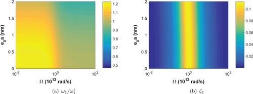
Figure 2. Nonlocal and viscoelastic effects on the second normalized undamped natural frequency ${\omega }_2/{\omega }_2^{\prime }$ (a) and damping ratio ${\zeta }_2$ (b).

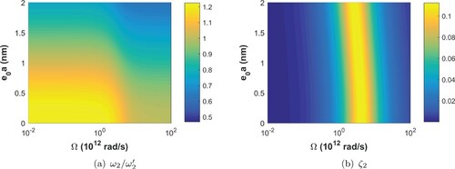
Figure 3. Nonlocal and viscoelastic effects on the third normalized undamped natural frequency ${\omega }_3/{\omega }_3^{\prime }$ (a) and damping ratio ${\zeta }_3$ (b).

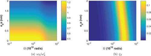
From Figures 1 to 3, one may observe that the nonlocal parameter $e_{0}a$ significantly affects the undamped natural frequencies of the system. An increase in the nonlocal parameter results in a decrease in the natural frequencies. Besides, the higher the mode, the greater the effect of $e_{0}a$ on the undamped natural frequency, showing that higher frequencies are more sensitive to small scale effects than the fundamental frequency. On the other hand, the effect of the nonlocal parameter on the damping ratios of the first three vibration modes is rather small. The damping ratios of the first two vibration modes remain practically constant with respect to $e_{0}a$.

Regarding the dependence of the modal properties with the viscoelastic parameter Ω, from Figures 1 to 3, one may observe that the undamped natural frequencies present a transition region when the viscoelastic parameter Ω is near the value of the corresponding natural frequency of a given mode [36]. Within the transition region, a decrease in the undamped natural frequencies is observed with an increase in the viscoelastic parameter Ω. Outside the transition region, the undamped natural frequencies present extremely low sensitivity with respect to the viscoelastic parameter Ω. On the other hand, Ω has a very significant effect on the damping ratios. One may observe that the damping ratios present a very pronounced ridge when Ω is in the vicinity of the corresponding natural frequency. Besides, the damping ratios monotonically decrease when Ω deviates from the value of the corresponding natural frequency. Small damping ratios are observed when Ω is far from the pronounced ridges.

4.2. Bayesian parameter estimation

This subsection is devoted to present some numerical analyses concerning the calibration of the nonlocal viscoelastic Euler-Bernoulli beam model of a simply supported SWCNT. Here, a model containing N = 1 internal variable is used to provide synthetic data for the inverse analyses.

The inverse problem is formulated considering the first three undamped natural frequencies and damping ratios of the system. The generalized response vector $\mathbf{y}$ is defined as follows (36) $\mathbf{y}={[{\omega }_1,{\omega }_2,{\omega }_3,{\zeta }_1,{\zeta }_2,{\zeta }_3]}^T$(36) where ${\omega }_r$ and ${\zeta }_r$ are, respectively, the undamped natural frequency and damping ratio of the rth vibration mode of the system.

Synthetic experimental modal data were computed considering the corrupting effects of noise as follows (37) ${\mathbf{y}}_E={\mathbf{y}}_{E0}+\mathit{ϵ}$(37) where ${\mathbf{y}}_{E0}$ is the reference generalized response vector, obtained considering the finite element model of the system and $\mathit{ϵ}$ is a zero-mean Gaussian random vector whose covariance matrix is ${\mathbf{\Sigma }}_{ϵϵ}$, i.e. $\mathit{ϵ}\sim \mathcal{N}(\mathbf{0},{\mathbf{\Sigma }}_{ϵϵ})$.

The modal parameters that compose the reference response vector ${\mathbf{y}}_{E0}$, presented in Table 5, were obtained considering the finite element model of the system and the parameters presented in Tables 1 and 4. Besides, the measurement error covariance matrix was assumed as follows (38) ${\mathbf{\Sigma }}_{ϵϵ}=\left[\begin{array}{cc}{\mathbf{\Sigma }}_{\omega \omega }& \mathbf{0}\\ \mathbf{0}& {\mathbf{\Sigma }}_{\zeta \zeta }\end{array}\right]$(38) where ${\mathbf{\Sigma }}_{\omega \omega }$ and ${\mathbf{\Sigma }}_{\zeta \zeta }$ are diagonal covariance matrices containing the variances of the measurement errors of the undamped natural frequencies and damping ratios, respectively. A relative standard deviation of 0.3% was adopted for the frequency measurement errors and a relative standard deviation of 3% was adopted for the measurement errors in the damping ratios. The standard deviations are relative to the corresponding reference values for the undamped natural frequencies and damping ratios presented in Table 5. It is worth mentioning that the relative values adopted for the standard deviations in the present manuscript are in agreement with experimental values found in the literature [54,55]. These assumptions yield ${\mathbf{\Sigma }}_{\omega \omega }=\text{diag}(0.16,1.75,5.60)$ GHz${}^2$ and ${\mathbf{\Sigma }}_{\zeta \zeta }=\text{diag}(4.60,0.51,0.16)\cdot {10}^{-6}$.

Table 4. Viscoelastic and nonlocal parameters adopted in the inverse problems of Cases 1 and 2.

Property	Symbol	Value
Nonlocal parameter (nm)	$e_{0}a$	1.5
Relaxation resistance	Δ	0.5
Inverse of relaxation time (rad/s)	Ω	$0.4\times {10}^{12}$

Table 5. Reference values for the undamped natural frequencies and damping ratios for Cases 1 and 2.

Mode	${\omega }_r$ (GHz)	${\zeta }_r$
1	134.25	0.072
2	441.12	0.024
3	788.86	0.013

Note: These modal parameters were computed considering the properties shown in Tables 1 and 4.

It should be highlighted that, in practice, the modal parameters of the system may be extracted from measured time domain data by means of the Eigensystem Realization Algorithm (ERA) [56], the Time Domain Decomposition method (TDD) [57] or the Subspace System Identification (SSI) [58], to cite a few.

Firstly, six cases were addressed in the numerical simulations, as summarized in Table 6. In Cases 1A, 1B and 1C, the nonlocal and the viscoelastic parameters were considered as unknowns, yielding the vector of unknown parameters $\mathit{\theta }=[e_{0}a,\mathrm{\Delta },\mathrm{\Omega }{]}^T$. Therefore, for cases 1A, 1B and 1C it is assumed that the diameter of the model, used along the inverse analyses, has a constant value and it is equal to a nominal value $d_0$. In particular, for case 1A one considers the nominal diameter $d_0$ for the inverse analysis exactly equal to the diameter d of the model that was used to generate the synthetic data, as shown in Table 1. On the other hand, for cases 1B and 1C one may analyze the impact of the misspecification of the system diameter value on the results provided by the inverse analyses. In Cases 2A, 2B and 2C, the diameter of the system was assumed as unknown and, therefore, it was also considered as a component of the vector of unknown model parameters, i.e. $\mathit{\theta }=[e_{0}a,\mathrm{\Delta },\mathrm{\Omega },d{]}^T$. In this case, as shown next, the prior densities for the diameter d were assumed as Gaussians centred at a nominal diameter value $d_0$. Different values for the nominal diameter of the SWCNT distinguish Cases 2A, 2B and 2C, as pinpointed in Table 6. Although the diameter d belongs to the vector of unknown parameters $\mathit{\theta }$, it should be highlighted that it consists of an uninteresting parameter.

Table 6. Cases 1 and 2 addressed in the inverse problem of parameter estimation.

		Diameter nominal	Unknown parameter
Case		value $d_0$ (nm)	vector ($\mathit{\theta }$)
	A	1.00
1	B	0.97	$[e_{0}a,\mathrm{\Delta },\mathrm{\Omega }{]}^T$
	C	1.03
	A	1.00
2	B	0.97	$[e_{0}a,\mathrm{\Delta },\mathrm{\Omega },d{]}^T$
	C	1.03

In the numerical results that follow, samples of the posterior probability density function of the unknown parameters were drawn by the DRAM algorithm. A total of $20\times {10}^3$ states were drawn, where the first $5\times {10}^3$ were considered as burn-in states. Two stages were considered. During the non-adaptation period $n_0=4\times {10}^3$ states, the covariance matrix of the auxiliary probability density function at the first stage was ${\mathbf{C}}_0$ (provided later, according to the considered case). The adaptation of the auxiliary density of the first stage started at the state $4\times {10}^3$ and the computation of the covariance matrix did not take into account the first $3\times {10}^3$ states of the burn-in period. At the second stage of the DRAM algorithm, which represents the DR step, the auxiliary density was obtained by scaling the auxiliary density of the first stage by a shrinking factor ${\gamma }_1=0.1$, as described in Subsection 3.1. The prior probability density functions and the initial states of the Markov chains are also provided later, according to the considered case.

4.2.1. Cases 1A, 1B and 1C

Numerical results regarding Cases 1A, 1B and 1C described in Table 6 are presented here. In these cases, the vector of unknown parameters is given by $\mathit{\theta }=[e_{0}a,\mathrm{\Delta },\mathrm{\Omega }{]}^T$.

The covariance matrix of the non-adaptation period of the DRAM was adopted as ${\mathbf{C}}_0=\text{diag}({\sigma }_1^2,{\sigma }_2^2,{\sigma }_3^2)$, with ${\sigma }_1=0.01$ nm, ${\sigma }_2=0.01$ and ${\sigma }_3=0.01\cdot {10}^{12}$ rad/s. During the adaptation period, the parameter $s_d=(2.4{)}^2/3$ was adopted, Equation (30(30) ${\mathbf{C}}_n^1=\{\begin{array}{ll}{\mathbf{C}}_0,& n\le n_0\\ s_d\text{Cov}({\mathit{\theta }}_0,{\mathit{\theta }}_1,\dots ,{\mathit{\theta }}_{n-1})+s_d\lambda {\mathbf{I}}_d,& n>n_0\end{array}$(30) ).

As for the prior density, it was assumed that all model parameters are independent random variables whose marginal densities are: $\pi (e_{0}a)=\mathcal{U}[0,2]$, $\pi (\mathrm{\Delta })=\mathcal{U}[0,1]$ and $\pi (\mathrm{\Omega })=\mathcal{U}[0,{10}^{13}]$. Here, $\mathcal{U}[a,b]$ is used to denote a uniform PDF defined within the interval $[a,b]$.

Figures 4–6 present the Markov chains and corresponding marginal posterior PDFs of the model parameters for Cases 1A, 1B and 1C.

Figure 4. (a) Markov Chains and (b) Marginal PDFs for $e_{0}a$ – Cases 1A, 1B and 1C. Note: dashed lines indicate the reference value.

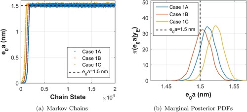
Figure 6. (a) Markov Chains and (b) Marginal PDFs for Ω – Cases 1A, 1B and 1C. Note: dashed lines indicate the reference value.

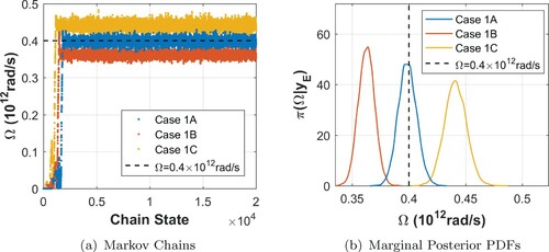
From Figures 4 to 6, one may observe that the chains converged to their stationary distributions and presented good mixing. In all cases considered in the present work, the convergence and mixing of the chains were verified by inspection of the cumulative mean values and autocorrelation functions of the unknown parameters, not shown here for the sake of space. Figure 4(a,b) show that the misspecification of the system diameter yielded extremely slight variations in the estimates of the nonlocal parameter $e_{0}a$, whose marginal PDFs presented approximately the same dispersion, in all cases, and all of them encompass the exact value of this parameter. Figures 5–6 pinpoint relatively biased solutions for the viscoelastic parameters Δ and Ω due to the adoption of a diameter $d_0$, for the inverse model, that is different from the one used to generate the synthetic experimental data. Although the PDFs of these parameters presented approximately the same dispersion, only those obtained from Case 1A encompass the corresponding exact values of these parameters.

Figure 5. (a) Markov Chains and (b) Marginal PDFs for Δ – Cases 1A, 1B and 1C. Note: dashed lines indicate the reference value.

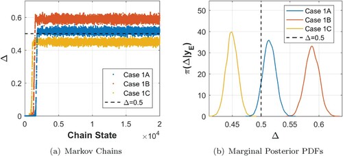
Table 7 presents the exact value of each estimated parameter, some corresponding sample statistical properties and the maximum a posteriori (MAP) estimate, obtained for Cases 1A, 1B and 1C. The considered sample statistics are: sample mean (μ), sample standard deviation (σ), coefficient of variation ($\sigma /\mu$) and 95% credibility interval ($\text{CI}95\mathrm{\%}$). The MAP estimate was obtained considering the Nelder-Mead optimization method [59].

Table 7. Parameter estimation results: Cases 1A, 1B and 1C.

Case	Parameter	Exact value	μ	σ	$\sigma /\mu$ $\mathrm{\%}$	CI 95$\mathrm{\%}$	MAP
	$e_{0}a$ (nm)	1.5	1.512	0.012	0.77	[1.489, 1.535]	1.512
1A	Δ	0.5	0.515	0.011	2.09	[0.494, 0.536]	0.515
	Ω (${10}^{12}$ rad/s)	0.4	0.399	0.008	2.03	[0.383, 0.415]	0.398
	$e_{0}a$ (nm)	1.5	1.504	0.012	0.80	[1.480, 1.527]	1.503
1B	Δ	0.5	0.588	0.012	2.02	[0.565, 0.611]	0.588
	Ω (${10}^{12}$ rad/s)	0.4	0.363	0.007	1.96	[0.349, 0.377]	0.363
	$e_{0}a$ (nm)	1.5	1.523	0.011	0.74	[1.501, 1.545]	1.523
1C	Δ	0.5	0.450	0.010	2.22	[0.430, 0.469]	0.449
	Ω (${10}^{12}$ rad/s)	0.4	0.441	0.010	2.17	[0.423, 0.460]	0.441

Relative errors around 18% and $-9\mathrm{\%}$, between the sample mean estimates and exact parameter values, for Δ and Ω, respectively, were obtained in Case 1B, when an error of $-3\mathrm{\%}$ in the system diameter was considered. Relative erros around $-10\mathrm{\%}$ and $10\mathrm{\%}$ for Δ and Ω, respectively, were obtained in Case 1C, where an error of $+3\mathrm{\%}$ in the system diameter was considered. Besides, the marginal PDFs of these parameters presented the greater coefficients of variation and the credibility intervals did not encompass their corresponding exact values.

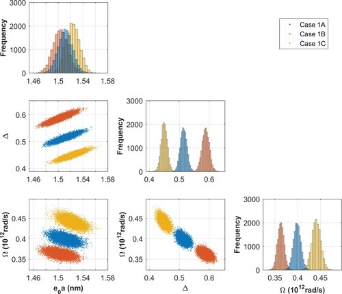
The marginal posterior distributions and the scatter plots of the model parameters, for Cases 1A, 1B and 1C, are presented in Figure 7, where one may observe a high correlation between the nonlocal parameter $e_{0}a$ and the viscoelastic parameter Δ. This correlation may be explained by the fact that, according to Figures 1–3, an increase in $e_{0}a$ yields a decrease in the values of the natural frequencies, whereas, on the other hand, the viscoelastic parameter Δ is related to the stiffness of the system, as can be observed in Equation (22(22) $\begin{array}{rl}& {\mathbf{M}}_e{\ddot{\mathbf{q}}}_e(t)+{\mathbf{D}}_e{\dot{\mathbf{q}}}_e(t)+[1+\sum _{i=1}^N{\mathrm{\Delta }}_i]{\mathbf{K}}_e{\mathbf{q}}_e(t)-{\mathbf{K}}_e\sum _{i=1}^N{\mathrm{\Delta }}_i{\overline{\mathbf{q}}}_{ei}(t)={\mathbf{P}}_e(t)\\ & \frac{{\mathrm{\Delta }}_i}{{\mathrm{\Omega }}_i}{\mathbf{K}}_e{\dot{\overline{\mathbf{q}}}}_{ei}(t)+{\mathrm{\Delta }}_i{\mathbf{K}}_e{\overline{\mathbf{q}}}_{ei}(t)-{\mathrm{\Delta }}_i{\mathbf{K}}_e{\mathbf{q}}_e(t)=\mathbf{0},i=1,2,\dots ,N\end{array}$(22) ), such that an increase in its value yields also an increase in the natural frequencies of the system. Therefore, in sampling the posterior probability density function of the unknown parameters, greater (smaller) values of $e_{0}a$ may be compensated by greater (smaller) values of Δ, and vice versa, as can be seen by the positive correlation between them in Figure 7.

Figure 7. Marginal posterior distributions (diagonal plots) and scatter plots of model parameters - Cases 1A, 1B and 1C.

4.2.2. Cases 2A, 2B and 2C – addressing misspecifications of the SWCNT diameter

In the results that follows, the diameter of the system is assumed uncertain and the vector of unknown parameters is defined as $\mathit{\theta }=[e_{0}a,\mathrm{\Delta },\mathrm{\Omega },d{]}^T$, according to Table 6.

The covariance matrix of the non-adaptation period of the DRAM was adopted as ${\mathbf{C}}_0=\text{diag}({\sigma }_1^2,{\sigma }_2^2,{\sigma }_3^2,{\sigma }_4^2)$, with ${\sigma }_1=0.01$ nm, ${\sigma }_2=0.01$, ${\sigma }_3=0.01\cdot {10}^{12}$ rad/s and ${\sigma }_4=0.01$ nm. During the adaptation period, the parameter $s_d=(2.4{)}^2/4$ was adopted, Equation (30(30) ${\mathbf{C}}_n^1=\{\begin{array}{ll}{\mathbf{C}}_0,& n\le n_0\\ s_d\text{Cov}({\mathit{\theta }}_0,{\mathit{\theta }}_1,\dots ,{\mathit{\theta }}_{n-1})+s_d\lambda {\mathbf{I}}_d,& n>n_0\end{array}$(30) ).

The same prior PDFs were adopted for the nonlocal and viscoelastic parameters: $\pi (e_{0}a)=\mathcal{U}[0,2]$, $\pi (\mathrm{\Delta })=\mathcal{U}[0,1]$ and $\pi (\mathrm{\Omega })=\mathcal{U}[0,{10}^{13}]$. Regarding the prior for d, it was assumed as $\pi (d)=\mathcal{N}(d_0,2.5\cdot {10}^{-3})$.

Figures 8, 9 and 10 present the Markov chains and marginal PDFs for the interesting parameters $\{e_{0}a,\mathrm{\Delta },\mathrm{\Omega }\}$ for cases 2A, 2B and 2C. It is interesting to note that the level of uncertainty provided by the marginal posteriors $\pi (e_{0}a|{\mathbf{y}}_E)$ is approximately the same as the one provided by the marginal posteriors in cases 1A, 1B and 1C, as shown in Figure 4.

Figure 8. (a) Markov Chains and (b) Marginal PDFs for $e_{0}a$ – Cases 2A, 2B and 2C. Note: dashed lines indicate the reference value.

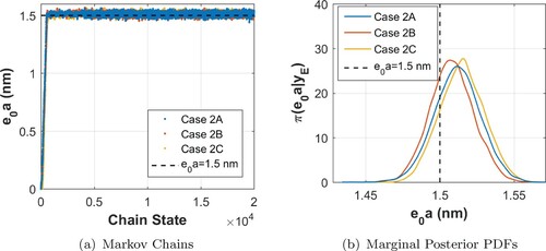
Figure 9. (a) Markov Chains and (b) Marginal PDFs for Δ – Cases 2A, 2B and 2C. Note: dashed lines indicate the reference value.

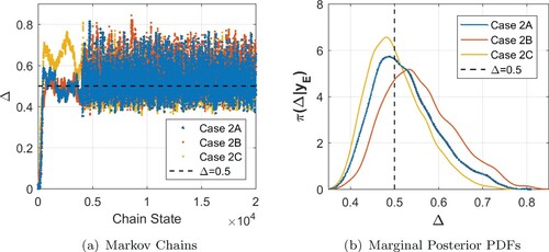
Figure 10. (a) Markov Chains and (b) Marginal PDFs for Ω – Cases 2A, 2B and 2C. Note: dashed lines indicate the reference value.

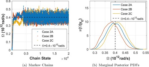
As for the viscoelastic parameters $\{\mathrm{\Delta },\mathrm{\Omega }\}$, Figures 9 and 10 indicate a larger level of uncertainty for them when compared to the one provided by the posteriors in cases 1A, 1B and 1C, as shown in Figures 5 and 6. Finally, Figure 11 presents the chains and marginal densities for the uninteresting parameter d.

Figure 11. (a) Markov Chains and (b) Marginal PDFs for d – Cases 2A, 2B and 2C. Note: dashed lines indicate the reference value.

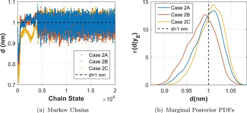
Figure 12 depicts the marginal posterior distributions, along with the scatter plots of the model parameters, for Cases 2A, 2B and 2C. High correlations between the parameters d, Δ and Ω may be clearly observed in Figure 12. The correlation between the parameters d and Δ may be explained as follows. The diameter d of the nanotube, similar to the viscoelastic parameter Δ, is related to the stiffness of the system. The higher the value of these parameters, the greater the stiffness and, consequently, the greater the natural frequencies of the system. Therefore, in sampling the posterior probability density function of the parameters, greater (smaller) values of d may be compensated by smaller (greater) values of Δ, and vice versa, yielding a negative correlation between them.

Figure 12. Marginal posterior distributions (diagonal plots) and scatter plots of model parameters – Cases 2A, 2B and 2C.

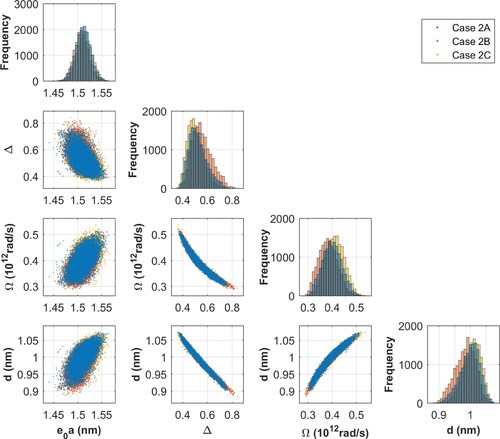
Table 8 presents some statical properties from cases 2A, 2B and 2C. An important aspect concerning the information presented in Table 8 and in the marginal PDFs shown in Figures 8, 9 and 10 is that, despite the fact that the level of uncertainty associated to the blue model parameters has increased, when compared to cases 1A, 1B and 1C, the true parameter values are within the feasible values provided by the posterior solutions of Cases 2A, 2B and 2C.

Table 8. Parameter estimation results: Cases 2A, 2B and 2C.

Case	Parameter	Exact value	μ	σ	$\sigma /\mu$ $\mathrm{\%}$	CI 95$\mathrm{\%}$	MAP
	$e_{0}a$ (nm)	1.5	1.512	0.016	1.02	[1.481, 1.542]	1.513
2A	Δ	0.5	0.524	0.073	13.91	[0.409, 0.695]	0.508
	Ω (${10}^{12}$ rad/s)	0.4	0.399	0.039	9.84	[0.325, 0.476]	0.403
	d (nm)	1.0	0.998	0.030	3.04	[0.931, 1.049]	1.003
	$e_{0}a$ (nm)	1.5	1.508	0.015	0.98	[1.480, 1.537]	1.509
2B	Δ	0.5	0.558	0.079	14.22	[0.429, 0.732]	0.537
	Ω (${10}^{12}$ rad/s)	0.4	0.382	0.038	9.95	[0.314, 0.459]	0.387
	d (nm)	1.0	0.984	0.036	3.20	[0.919, 1.038]	0.991
	$e_{0}a$ (nm)	1.5	1.515	0.015	0.98	[1.486, 1.544]	1.517
2C	Δ	0.5	0.503	0.064	12.74	[0.401, 0.647]	0.485
	Ω (${10}^{12}$ rad/s)	0.4	0.411	0.038	9.17	[0.340, 0.485]	0.417
	d (nm)	1.0	1.006	0.027	2.73	[0.947, 1.053]	1.013

From these analyses one may observe that slight levels of misspecification in the system diameter may lead to significant biased estimates for the viscoelastic parameters $\{\mathrm{\Delta },\mathrm{\Omega }\}$, as shown in Figures 5 and 6, when one does not consider the diameter as an uncertain model parameter. At the same time, when assuming the diameter as an unknown but uninteresting model parameter, this biased characteristic could be properly alleviated.

It is worth mentioning the fact that, in this subsection, the model used for inversion analyses is able to describe the entire physical mechanisms associated to the model that provided the set of synthetic data. Nevertheless, in practice one will likely face situations where the model used for inversion is not able to completely describe the damping/dissipative mechanisms present in the system. This issue will be approached in Subsection 4.3, shown next using a preliminary approach.

4.3. Further analysis

In order to simulate a more realistic situation, in the following analysis, the nonlocal viscoelastic beam model with N = 1 internal variable is calibrated in the presence of both measurement and modelling errors. The modelling error here stems from the incomplete modelling of the damping mechanisms of the system. More specifically, one considers a model with $\overline{N}=2$ internal variables to provide the reference data ${\mathbf{y}}_{E0}$ for computing the synthetic experimental data ${\mathbf{y}}_E$, whereas a forward model with N = 1 internal variable is used for the inverse analysis.

Given the fact that the model used to derive the synthetic data and the one used in the inverse analysis are different, one may rewrite the observation model, relating observations ${\mathbf{y}}_E$ and model predictions, as follows [60] (39) $\begin{array}{rl}{\mathbf{y}}_E& =\overline{\mathbf{A}}(\overline{\mathit{\theta }})+\mathit{ϵ}=\mathbf{A}(\mathit{\theta })+\mathit{ϵ}+[\overline{\mathbf{A}}(\overline{\mathit{\theta }})-\mathbf{A}(\mathit{\theta })]\\ & =\mathbf{A}(\mathit{\theta })+\mathit{ϵ}+\mathit{\eta }(\overline{\mathit{\theta }},\mathit{\theta })\\ & =\mathbf{A}(\mathit{\theta })+\widetilde{\mathit{ϵ}}\end{array}$(39) where $\overline{\mathbf{A}}(\overline{\mathit{\theta }})$ is an accurate forward operator able to completely describe the physical mechanisms associated to the system under analysis, such that discrepancies between measured data ${\mathbf{y}}_E$ and model predictions could be completely described by measurement errors $\mathit{ϵ}$. The accurate forward operator in Equation (39(39) $\begin{array}{rl}{\mathbf{y}}_E& =\overline{\mathbf{A}}(\overline{\mathit{\theta }})+\mathit{ϵ}=\mathbf{A}(\mathit{\theta })+\mathit{ϵ}+[\overline{\mathbf{A}}(\overline{\mathit{\theta }})-\mathbf{A}(\mathit{\theta })]\\ & =\mathbf{A}(\mathit{\theta })+\mathit{ϵ}+\mathit{\eta }(\overline{\mathit{\theta }},\mathit{\theta })\\ & =\mathbf{A}(\mathit{\theta })+\widetilde{\mathit{ϵ}}\end{array}$(39) ) requires the specification of its own set of parameters $\overline{\mathit{\theta }}$. As for the right side of Equation (39(39) $\begin{array}{rl}{\mathbf{y}}_E& =\overline{\mathbf{A}}(\overline{\mathit{\theta }})+\mathit{ϵ}=\mathbf{A}(\mathit{\theta })+\mathit{ϵ}+[\overline{\mathbf{A}}(\overline{\mathit{\theta }})-\mathbf{A}(\mathit{\theta })]\\ & =\mathbf{A}(\mathit{\theta })+\mathit{ϵ}+\mathit{\eta }(\overline{\mathit{\theta }},\mathit{\theta })\\ & =\mathbf{A}(\mathit{\theta })+\widetilde{\mathit{ϵ}}\end{array}$(39) ), it explicitly states that if one decides to write the observation model using a less accurate predictive model $\mathbf{A}(\mathit{\theta })$, one should take into account the modelling errors, defined as $\mathit{\eta }=\overline{\mathbf{A}}(\overline{\mathit{\theta }})-\mathbf{A}(\mathit{\theta })$. Besides, according to Equation (39(39) $\begin{array}{rl}{\mathbf{y}}_E& =\overline{\mathbf{A}}(\overline{\mathit{\theta }})+\mathit{ϵ}=\mathbf{A}(\mathit{\theta })+\mathit{ϵ}+[\overline{\mathbf{A}}(\overline{\mathit{\theta }})-\mathbf{A}(\mathit{\theta })]\\ & =\mathbf{A}(\mathit{\theta })+\mathit{ϵ}+\mathit{\eta }(\overline{\mathit{\theta }},\mathit{\theta })\\ & =\mathbf{A}(\mathit{\theta })+\widetilde{\mathit{ϵ}}\end{array}$(39) ), one has that the difference between measured data ${\mathbf{y}}_E$ and predictions provided by a less accurate operator $\mathbf{A}(\mathit{\theta })$ depends on both measurement errors $\mathit{ϵ}$ and modelling errors $\mathit{\eta }$. One aspect that should be emphasized is the fact that the modelling errors $\mathit{\eta }$ depend on the structure of the model $\mathbf{A}(\mathit{\theta })$ and also on the structure of the accurate model $\overline{\mathbf{A}}(\overline{\mathit{\theta }})$.

In the present case, as the models $\overline{\mathbf{A}}(\overline{\mathit{\theta }})$ and $\mathbf{A}(\mathit{\theta })$ belong to different model classes, inasmuch as $\overline{\mathbf{A}}(\overline{\mathit{\theta }})$ is built with $\overline{N}=2$ internal variables and $\mathbf{A}(\mathit{\theta })$ is built with N = 1 internal variable, a simplifying hypothesis was adopted here which proved amenable for the present application. It was assumed that the effects of the measurement errors $\mathit{ϵ}$ and modelling errors $\mathit{\eta }$ could be globally described by a single random variable $\widetilde{\mathit{ϵ}}$, as shown in Equation (39(39) $\begin{array}{rl}{\mathbf{y}}_E& =\overline{\mathbf{A}}(\overline{\mathit{\theta }})+\mathit{ϵ}=\mathbf{A}(\mathit{\theta })+\mathit{ϵ}+[\overline{\mathbf{A}}(\overline{\mathit{\theta }})-\mathbf{A}(\mathit{\theta })]\\ & =\mathbf{A}(\mathit{\theta })+\mathit{ϵ}+\mathit{\eta }(\overline{\mathit{\theta }},\mathit{\theta })\\ & =\mathbf{A}(\mathit{\theta })+\widetilde{\mathit{ϵ}}\end{array}$(39) ), and that it follows a zero mean Gaussian density function, i.e. $\widetilde{\mathit{ϵ}}\sim \mathcal{N}(\mathbf{0},{\mathbf{\Sigma }}_{\widetilde{ϵ}\widetilde{ϵ}})$, where ${\mathbf{\Sigma }}_{\widetilde{ϵ}\widetilde{ϵ}}$ is unknown. Further, for the inverse analysis it is assumed that $\mathit{\theta }$ and the global error $\widetilde{\mathit{ϵ}}$ are independent random variables, such that the likelihood function may be written as (40) $\pi ({\mathbf{y}}_E|\mathit{\theta })=\frac{1}{\sqrt{(2\pi {)}^{N_y}}\sqrt{det\left({\mathbf{\Sigma }}_{\widetilde{ϵ}\widetilde{ϵ}}\right)}}\exp [-\frac{1}{2}{({\mathbf{y}}_E-\mathbf{A}\mathbf{(}\mathit{\theta }\mathbf{)})}^T{\mathbf{\Sigma }}_{\widetilde{ϵ}\widetilde{ϵ}}^{-1}({\mathbf{y}}_E-\mathbf{A}\mathbf{(}\mathit{\theta }\mathbf{)})]$(40) Finally, given the fact that the vector ${\mathbf{y}}_E$ contains information of measured natural frequencies and damping ratios, one decided for a parameterization of the covariance matrix ${\mathbf{\Sigma }}_{\widetilde{ϵ}\widetilde{ϵ}}$ as follows (41) ${\mathbf{\Sigma }}_{\widetilde{ϵ}\widetilde{ϵ}}={\beta }^2{\mathbf{\Sigma }}_{ϵϵ}$(41) where β is an unknown parameter and the matrix ${\mathbf{\Sigma }}_{ϵϵ}$ is the covariance matrix of the measurement errors $\mathit{ϵ}$ shown in Equation (38(38) ${\mathbf{\Sigma }}_{ϵϵ}=\left[\begin{array}{cc}{\mathbf{\Sigma }}_{\omega \omega }& \mathbf{0}\\ \mathbf{0}& {\mathbf{\Sigma }}_{\zeta \zeta }\end{array}\right]$(38) ).

In the present case (Case 3), the modal parameters that compose the reference response vector ${\mathbf{y}}_{E0}$ were obtained considering a model built with $\overline{N}=2$ internal variables, whose parameters are presented in Tables 1 and 9. The reference modal parameters for Case 3 are presented in Table 10. As in the previous cases, the experimental response vector ${\mathbf{y}}_E$ was computed considering a relative standard deviation of 0.3% for the frequency errors and a relative standard deviation of 3% for the errors in the damping ratios. The standard deviations are relative to the corresponding reference values for the undamped natural frequencies and damping ratios presented in Table 10, yielding ${\mathbf{\Sigma }}_{\omega \omega }=\text{diag}(0.16,1.87,6.47)$ GHz${}^2$ and ${\mathbf{\Sigma }}_{\zeta \zeta }=\text{diag}(8.12,6.49,7.11)\cdot {10}^{-6}$.

Table 9. Viscoelastic and nonlocal parameters adopted to generate the synthetic data in Case 3.

Property	Symbol	Value
Nonlocal parameter (nm)	$e_{0}a$	1.5
Relaxation resistance 1	${\mathrm{\Delta }}_1$	0.5
Inverse of relaxation time 1 (rad/s)	${\mathrm{\Omega }}_1$	$0.4\times {10}^{12}$
Relaxation resistance 2	${\mathrm{\Delta }}_2$	0.5
Inverse of relaxation time 2 (rad/s)	${\mathrm{\Omega }}_2$	$6.3\times {10}^{12}$

Table 10. Reference values for the undamped natural frequencies and damping ratios for Case 3.

Mode	${\omega }_r$ (GHz)	${\zeta }_r$
1	135.11	0.095
2	455.56	0.085
3	847.97	0.089

Note: These modal parameters were computed considering the properties shown in Tables 1 and 9.

The nonlocal $e_{0}a$ and viscoelastic parameters $\{\mathrm{\Delta },\mathrm{\Omega }\}$, along with the nanotube diameter d and the parameter β, related to the covariance matrix of the global error vector $\widetilde{\mathit{ϵ}}$, Equation (41(41) ${\mathbf{\Sigma }}_{\widetilde{ϵ}\widetilde{ϵ}}={\beta }^2{\mathbf{\Sigma }}_{ϵϵ}$(41) ), were considered as unknowns in Case 3, i.e. the vector of unknown parameters is $\mathit{\theta }=[e_{0}a,\mathrm{\Delta },\mathrm{\Omega },d,\beta {]}^T$, as indicated in Table 11.

Table 11. Case 3 addressed in the inverse problem of parameter estimation.

	Diameter nominal	Unknown parameter
Case	value $d_0$ (nm)	vector ($\mathit{\theta }$)
3	1.00	$[e_{0}a,\mathrm{\Delta },\mathrm{\Omega },d,\beta {]}^T$

Concerning the prior probability density function, it was built assuming the unknown parameters as independent random variables whose marginal densities are: $\pi (e_{0}a)=\mathcal{U}[0,2]$, $\pi (\mathrm{\Delta })=\mathcal{U}[0,2]$, $\pi (\mathrm{\Omega })=\mathcal{U}[0,{10}^{13}]$, $\pi (d)=\mathcal{N}(1,2.5\cdot {10}^{-3})$ and $\pi ({\beta }^2)=\mathcal{I}\mathcal{G}(9.5,11.1)$, where $\mathcal{I}\mathcal{G}(a,b)$ stands for the inverse gamma distribution, with shape parameter a and scale parameter b. As for the sampling of the posterior probability density function, it was considered $2\times {10}^5$ samples where the first $3\times {10}^4$ ones were considered as burn-in states.

Figure 13 depicts the marginal posterior distributions, along with the scatter plots of the model parameters, obtained for Case 3. Regarding the marginal posterior distributions shown in Figure 13, one may highlight the fact that comparisons between feasible values and reference ones may be meaningless, except for the nonlocal parameter $e_{0}a$. This is due to the fact that the nonlocal parameter $e_{0}a$ is the only constitutive model parameter with the same physical meaning in the model with N = 1 internal variable, used for the inverse analysis, and in the model with $\overline{N}=2$ internal variables, used to generate the synthetic data.

Figure 13. Marginal posterior distributions (diagonal plots) and scatter plots of model parameters – Case 3.

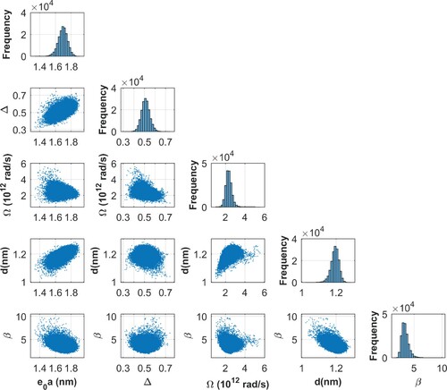
Table 12 presents the statistical properties of the model parameters provided by the inverse analysis. From Table 12, one may observe that the reference value of the nonlocal parameter $e_{0}a$ is not within the 95% credibility interval. However, the reference value of the nonlocal parameter is within the feasible region provided by the posterior marginal density $\pi (e_{0}a|{\mathbf{y}}_E)$, as can be seen from Figure 13. Regarding the scaling parameter β, which is used in Equation (41(41) ${\mathbf{\Sigma }}_{\widetilde{ϵ}\widetilde{ϵ}}={\beta }^2{\mathbf{\Sigma }}_{ϵϵ}$(41) ) to characterize the covariance of the random errors $\widetilde{\mathit{ϵ}}$ in Equation (39(39) $\begin{array}{rl}{\mathbf{y}}_E& =\overline{\mathbf{A}}(\overline{\mathit{\theta }})+\mathit{ϵ}=\mathbf{A}(\mathit{\theta })+\mathit{ϵ}+[\overline{\mathbf{A}}(\overline{\mathit{\theta }})-\mathbf{A}(\mathit{\theta })]\\ & =\mathbf{A}(\mathit{\theta })+\mathit{ϵ}+\mathit{\eta }(\overline{\mathit{\theta }},\mathit{\theta })\\ & =\mathbf{A}(\mathit{\theta })+\widetilde{\mathit{ϵ}}\end{array}$(39) ), one may observe that its marginal posterior distribution is centred around 4. This fact indicates that the support of the likelihood function had to expand in order to cope with the discrepancies associated to the modelling error that stemmed from the fact that the model used in the inverse analysis is not able to completely describe the dissipation mechanisms associated to the system that provided the synthetic data.

Table 12. Parameter estimation results: Case 3.

Parameter	Exact value	μ	σ	$\sigma /\mu$ $\mathrm{\%}$	CI 95$\mathrm{\%}$	MAP
$e_{0}a$ (nm)	1.5	1.694	0.059	3.50	[1.568, 1.804]	1.713
Δ	–	0.511	0.040	7.75	[0.436, 0.592]	0.512
Ω (${10}^{12}$ rad/s)	–	2.335	0.312	13.34	[1.788, 3.011]	2.322
d (nm)	1	1.193	0.023	1.93	[1.143, 1.234]	1.201
β	–	3.398	0.630	18.53	[2.456, 4.864]	2.871

As a final comment concerning Case 3, one may highlight that the adopted approach could be used when the user cannot properly select an accurate model to completely describe the dissipation mechanisms of the system under analysis. In this perspective, this simple approach could be used as an alternative to build an equivalent model for predictive analyses, when considering the simplifying hypothesis of a zero mean Gaussian global error $\widetilde{\mathit{ϵ}}$ in Equation (39(39) $\begin{array}{rl}{\mathbf{y}}_E& =\overline{\mathbf{A}}(\overline{\mathit{\theta }})+\mathit{ϵ}=\mathbf{A}(\mathit{\theta })+\mathit{ϵ}+[\overline{\mathbf{A}}(\overline{\mathit{\theta }})-\mathbf{A}(\mathit{\theta })]\\ & =\mathbf{A}(\mathit{\theta })+\mathit{ϵ}+\mathit{\eta }(\overline{\mathit{\theta }},\mathit{\theta })\\ & =\mathbf{A}(\mathit{\theta })+\widetilde{\mathit{ϵ}}\end{array}$(39) ). From this point of view, the raw examination of the samples $\mathit{\theta }\sim \pi (\mathit{\theta }|{\mathbf{y}}_E)$ may possibly not be useful. 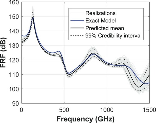Nevertheless, the analysis of model predictions $\mathbf{z}(\mathit{\theta })$ provided by the equivalent model, for diverse conditions, when $\mathit{\theta }\sim \pi (\mathit{\theta }|{\mathbf{y}}_E)$ may prove useful. In this sense, as an example, one decided to analyze the predictions provided by the calibrated model when the quantity of interest is the Frequency Response Function (FRF) of the nonlocal viscoelastic beam, i.e. $z(\mathit{\theta })=H(\mathit{\theta };\omega )$, where ω is the angular frequency. The FRF relating an excitation at position 0.45 nm with the displacement of the system at 0.85 nm is considered here. Figure 14 depicts the FRF provided by the reference model with $\overline{N}=2$ internal variables in blue line. The model with N = 1 internal variable is used to provide model predictions $z(\mathit{\theta })=H(\mathit{\theta };\omega )$, using samples $\{{\mathit{\theta }}_1,{\mathit{\theta }}_2,\dots \}$ (after discarding the brun-in states) from the posterior probability density $\pi (\mathit{\theta }|{\mathbf{y}}_E)$ obtained for Case 3. Realizations of model predictions $z(\mathit{\theta })=H(\mathit{\theta };\omega )$ are shown in grey lines and the black line indicates its expected values; moreover, dashed lines indicate the 99% stochastic envelope provided by the model predictions. From Figure 14 one may observe that the stochastic envelope provided by the model with N = 1 internal variable encompasses the FRF provided by the reference model with $\overline{N}=2$ internal variables until the fourth mode of the system, around 1250 GHz.

Figure 14. Frequency Response Function of the reference model along with the mean and 99% credibility interval predicted by the model used in the inversion.

Concerning the calibration of a model containing N = 1 internal variable, assuming the conventional observation model, i.e. $\beta =1$ in Equation (41(41) ${\mathbf{\Sigma }}_{\widetilde{ϵ}\widetilde{ϵ}}={\beta }^2{\mathbf{\Sigma }}_{ϵϵ}$(41) ), although it is not shown here one states that: (i) its model predictions $z(\mathit{\theta })=H(\mathit{\theta };\omega )$ present quite low levels of uncertainty when compared to the ones shown in Figure 14, and (ii) it fails to properly describe the second and fourth modes of the system under analysis.

Finally, one should notice that the choice for this simplifying approach in the presence of modelling errors $\mathit{\eta }$ is an attempt to build an equivalent predictive model for the system under analysis. More rigorous and comprehensive approaches could be considered aiming at obtaining an accurate calibrated model and its proper parameter estimates. This requires that the user has candidate feasible models that are believed to accurately describe the physical mechanisms inherent to the system under analysis. In this sense, as an example, one may cite the approach proposed by Muto and Beck [61], where a set of feasible models $\{{\mathcal{M}}_1,{\mathcal{M}}_2,\dots ,{\mathcal{M}}_{\overline{m}}\}$ of $\overline{m}$ different classes are assessed and the probability of each model $\mathbb{P}({\mathcal{M}}_r|{\mathbf{y}}_E)$, given a set of measured data ${\mathbf{y}}_E$, is computed taking into account a balance between its predictive capabilities and its complexity. This approach would be interesting in case the user has, for example, model classes describing different dissipations mechanisms or even different numbers of internal variables, but he is unable, at a first sight, to specify which model would be the most appropriate one to describe the physical phenomena of the system under analysis.

5. Conclusions

The present work presented a model for nonlocal and viscoelastic Euler-Bernoulli beams and some aspects of the calibration of its nonlocal viscoleastic model were addressed. The inverse analyses was performed based on the Bayesian framework. The main contributions of the present work are:

• to present an approach to simultaneously estimate the nonlocal $e_{0}a$ and viscoelastic $\{\mathrm{\Delta },\mathrm{\Omega }\}$ constitutive model parameters;

• to assess the impact of a misspecification of the beam diameter d on the estimation of the constitutive parameters $\{e_{0}a,\mathrm{\Delta },\mathrm{\Omega }\}$ and its compensation when considering d as an unknown but uninteresting parameter;

• to build an equivalent model to describe more complex damping mechanisms than the one inherent to the model with N = 1 internal variable, based on the hypothesis that the model errors could be described by means of a zero mean Gaussian global error with unknown covariance matrix.

• to show that the equivalent predictive model is somehow able to describe the response of the system under analysis when the global error model is calibrated.

Disclosure statement

No potential conflict of interest was reported by the author(s).

Additional information

Funding

This study was financed in part by the Coordenação de Aperfeiçoamento de Pessoal de Nível Superior - (CAPES/Brasil) under Finance Code 001, by Fundação Carlos Chagas Filho de Amparo á Pesquisa do Estado do Rio de Janeiro (FAPERJ) and by Conselho Nacional de Desenvolvimento Científico e Tecnológico (CNPq) under grant number 304773/2017-4 and 210.360/2019.

Appendices

Appendix 1.

Finite element matrices and vectors

The vector of generalized element nodal displacements and the vector of internal variables are, respectively, defined as (A1) $\begin{array}{rl}& {\mathbf{q}}_e=\left[\begin{array}{c}{q}_{e1}\\ q_{e2}\\ q_{e3}\\ q_{e4}\end{array}\right]\end{array}$(A1) (A2) $\begin{array}{rl}& {\overline{\mathbf{q}}}_{ei}=\left[\begin{array}{c}{\overline{q}}_{ei1}\\ {\overline{q}}_{ei2}\\ {\overline{q}}_{ei3}\\ {\overline{q}}_{ei4}\end{array}\right]\end{array}$(A2) where $q_{e1}$ and $q_{e3}$ are transverse displacements and $q_{e2}$ and $q_{e4}$ are rotations at the element nodes.

The matrix with the interpolation functions is given by (A3) $\mathbf{N}(\overline{x})=\left[\begin{array}{c}{\displaystyle \frac{2{\overline{x}}^3}{{l_e}^3}}-{\displaystyle \frac{3{\overline{x}}^2}{{l_e}^2}}+1\\ {\displaystyle \frac{{\overline{x}}^3}{{l_e}^2}}-{\displaystyle \frac{2{\overline{x}}^2}{l_e}}+\overline{x}\\ {\displaystyle \frac{3{\overline{x}}^2}{{l_e}^2}}-{\displaystyle \frac{2{\overline{x}}^3}{{l_e}^3}}\\ {\displaystyle \frac{{\overline{x}}^3}{{l_e}^2}}-{\displaystyle \frac{{\overline{x}}^2}{l_e}}\end{array}\right]$(A3) The element mass matrix is defined as (A4) ${\mathbf{M}}_e=\rho A{\int }_0^{l_e}\mathbf{N}(\overline{x}){\mathbf{N}}^T(\overline{x})\mathrm{d}\overline{x}+\rho A(e_{0}a{)}^2{\int }_0^{l_e}\frac{\mathrm{d}\mathbf{N}(\overline{x})}{\mathrm{d}\overline{x}}\frac{\mathrm{d}{\mathbf{N}}^T(\overline{x})}{\mathrm{d}\overline{x}}\mathrm{d}\overline{x}$(A4) The element viscous damping matrix is defined as (A5) ${\mathbf{D}}_e=C{\int }_0^{l_e}\mathbf{N}(\overline{x}){\mathbf{N}}^T(\overline{x})\mathrm{d}\overline{x}+C(e_{0}a{)}^2{\int }_0^{l_e}\frac{\mathrm{d}\mathbf{N}(\overline{x})}{\mathrm{d}\overline{x}}\frac{\mathrm{d}{\mathbf{N}}^T(\overline{x})}{\mathrm{d}\overline{x}}\mathrm{d}\overline{x}$(A5) The relaxed stiffness matrix is defined as (A6) ${\mathbf{K}}_e=E_{\mathrm{\infty }}I{\int }_0^{l_e}\frac{{\mathrm{\partial }}^2\mathbf{N}(\overline{x})}{\mathrm{\partial }{\overline{x}}^2}\frac{{\mathrm{\partial }}^2{\mathbf{N}}^T(\overline{x})}{\mathrm{\partial }{\overline{x}}^2}\mathrm{d}\overline{x}$(A6) The vector of generalized nodal forces is defined as (A7) ${\mathbf{P}}_e(t)={\int }_0^{l_e}(\mathbf{N}(\overline{x})-(e_{0}a{)}^2\frac{{\mathrm{\partial }}^2\mathbf{N}(\overline{x})}{\mathrm{\partial }{\overline{x}}^2})f(t)\mathrm{d}\overline{x}$(A7)

Appendix 2.

State-space model and system poles

Taking into account the elemental equations in (22(22) $\begin{array}{rl}& {\mathbf{M}}_e{\ddot{\mathbf{q}}}_e(t)+{\mathbf{D}}_e{\dot{\mathbf{q}}}_e(t)+[1+\sum _{i=1}^N{\mathrm{\Delta }}_i]{\mathbf{K}}_e{\mathbf{q}}_e(t)-{\mathbf{K}}_e\sum _{i=1}^N{\mathrm{\Delta }}_i{\overline{\mathbf{q}}}_{ei}(t)={\mathbf{P}}_e(t)\\ & \frac{{\mathrm{\Delta }}_i}{{\mathrm{\Omega }}_i}{\mathbf{K}}_e{\dot{\overline{\mathbf{q}}}}_{ei}(t)+{\mathrm{\Delta }}_i{\mathbf{K}}_e{\overline{\mathbf{q}}}_{ei}(t)-{\mathrm{\Delta }}_i{\mathbf{K}}_e{\mathbf{q}}_e(t)=\mathbf{0},i=1,2,\dots ,N\end{array}$(22) ), the equations of motion of a nonlocal viscoelastic Euler-Bernoulli beam can be written as (A8) $\begin{array}{rl}& \mathbf{M}\ddot{\mathbf{q}}(t)+\mathbf{D}\dot{\mathbf{q}}(t)+[1+\sum _{i=1}^N{\mathrm{\Delta }}_i]\mathbf{K}\mathbf{q}(t)-\mathbf{K}\sum _{i=1}^N{\mathrm{\Delta }}_i{\overline{\mathbf{q}}}_i(t)=\mathbf{P}(t)\\ & \frac{{\mathrm{\Delta }}_1}{{\mathrm{\Omega }}_1}\mathbf{K}{\dot{\overline{\mathbf{q}}}}_1(t)+{\mathrm{\Delta }}_1\mathbf{K}{\overline{\mathbf{q}}}_1(t)-{\mathrm{\Delta }}_1\mathbf{K}\mathbf{q}(t)=\mathbf{0}\\ & \frac{{\mathrm{\Delta }}_2}{{\mathrm{\Omega }}_2}\mathbf{K}{\dot{\overline{\mathbf{q}}}}_2(t)+{\mathrm{\Delta }}_2\mathbf{K}{\overline{\mathbf{q}}}_2(t)-{\mathrm{\Delta }}_2\mathbf{K}\mathbf{q}(t)=\mathbf{0}\\ & ⋮\\ & \frac{{\mathrm{\Delta }}_N}{{\mathrm{\Omega }}_N}\mathbf{K}{\dot{\overline{\mathbf{q}}}}_N(t)+{\mathrm{\Delta }}_N\mathbf{K}{\overline{\mathbf{q}}}_N(t)-{\mathrm{\Delta }}_N\mathbf{K}\mathbf{q}(t)=\mathbf{0}\end{array}$(A8) Defining the augmented displacement vector as (A9) ${\mathbf{q}}_a(t)=\left[\begin{array}{c}\mathbf{q}(t)\\ {\overline{\mathbf{q}}}_1(t)\\ ⋮\\ {\overline{\mathbf{q}}}_N(t)\end{array}\right]$(A9) the coupled equations in (A8(A8) $\begin{array}{rl}& \mathbf{M}\ddot{\mathbf{q}}(t)+\mathbf{D}\dot{\mathbf{q}}(t)+[1+\sum _{i=1}^N{\mathrm{\Delta }}_i]\mathbf{K}\mathbf{q}(t)-\mathbf{K}\sum _{i=1}^N{\mathrm{\Delta }}_i{\overline{\mathbf{q}}}_i(t)=\mathbf{P}(t)\\ & \frac{{\mathrm{\Delta }}_1}{{\mathrm{\Omega }}_1}\mathbf{K}{\dot{\overline{\mathbf{q}}}}_1(t)+{\mathrm{\Delta }}_1\mathbf{K}{\overline{\mathbf{q}}}_1(t)-{\mathrm{\Delta }}_1\mathbf{K}\mathbf{q}(t)=\mathbf{0}\\ & \frac{{\mathrm{\Delta }}_2}{{\mathrm{\Omega }}_2}\mathbf{K}{\dot{\overline{\mathbf{q}}}}_2(t)+{\mathrm{\Delta }}_2\mathbf{K}{\overline{\mathbf{q}}}_2(t)-{\mathrm{\Delta }}_2\mathbf{K}\mathbf{q}(t)=\mathbf{0}\\ & ⋮\\ & \frac{{\mathrm{\Delta }}_N}{{\mathrm{\Omega }}_N}\mathbf{K}{\dot{\overline{\mathbf{q}}}}_N(t)+{\mathrm{\Delta }}_N\mathbf{K}{\overline{\mathbf{q}}}_N(t)-{\mathrm{\Delta }}_N\mathbf{K}\mathbf{q}(t)=\mathbf{0}\end{array}$(A8) ) may be expressed in the compact form [46] (A10) ${\mathbf{M}}_a{\ddot{\mathbf{q}}}_a(t)+{\mathbf{D}}_a{\dot{\mathbf{q}}}_a(t)+{\mathbf{K}}_a{\mathbf{q}}_a(t)={\mathbf{P}}_a(t)$(A10) where (A11) ${\mathbf{M}}_a=\left[\begin{array}{cc}\mathbf{M}& \mathbf{0}\\ \mathbf{0}& \mathbf{0}\end{array}\right],{\mathbf{D}}_a=\left[\begin{array}{cc}\mathbf{D}& \mathbf{0}\\ \mathbf{0}& {\mathbf{D}}_a^{22}\end{array}\right],{\mathbf{K}}_a=\left[\begin{array}{cc}{\mathbf{K}}_a^{11}& {\mathbf{K}}_a^{12}\\ {\mathbf{K}}_a^{21}& {\mathbf{K}}_a^{22}\end{array}\right],{\mathbf{P}}_a=\left[\begin{array}{c}\mathbf{P}(t)\\ \mathbf{0}\\ ⋮\\ \mathbf{0}\end{array}\right]$(A11) with (A12) $\begin{array}{rl}{\mathbf{D}}_a^{22}& =\left[\begin{array}{cccc}{\displaystyle \frac{{\mathrm{\Delta }}_1}{{\mathrm{\Omega }}_1}}\mathbf{K}& \mathbf{0}& \dots & \mathbf{0}\\ \mathbf{0}& {\displaystyle \frac{{\mathrm{\Delta }}_2}{{\mathrm{\Omega }}_2}}\mathbf{K}& \dots & \mathbf{0}\\ ⋮& ⋮& \ddots & ⋮\\ \mathbf{0}& \mathbf{0}& \dots & {\displaystyle \frac{{\mathrm{\Delta }}_N}{{\mathrm{\Omega }}_N}}\mathbf{K}\end{array}\right]\\ {\mathbf{K}}_a^{11}& =(1+\sum _{i=1}^N{\mathrm{\Delta }}_i)\mathbf{K}\\ {\mathbf{K}}_a^{12}& =[-{\mathrm{\Delta }}_1\mathbf{K},\dots ,-{\mathrm{\Delta }}_N\mathbf{K}]\\ {\mathbf{K}}_a^{21}& ={\left[{\mathbf{K}}_a^{12}\right]}^T\\ {\mathbf{K}}_a^{22}& =\left[\begin{array}{cccc}{\mathrm{\Delta }}_1\mathbf{K}& \mathbf{0}& \dots & \mathbf{0}\\ \mathbf{0}& {\mathrm{\Delta }}_2\mathbf{K}& \dots & \mathbf{0}\\ ⋮& ⋮& \ddots & ⋮\\ \mathbf{0}& \mathbf{0}& \dots & {\mathrm{\Delta }}_N\mathbf{K}\end{array}\right]\end{array}$(A12) Defining the augmented state vector (A13) ${\mathbf{x}}_a(t)=\left[\begin{array}{c}{\mathbf{q}}_a(t)\\ \dot{\mathbf{q}}(t)\end{array}\right]$(A13) the second-order equation of motion in Equation (A10(A10) ${\mathbf{M}}_a{\ddot{\mathbf{q}}}_a(t)+{\mathbf{D}}_a{\dot{\mathbf{q}}}_a(t)+{\mathbf{K}}_a{\mathbf{q}}_a(t)={\mathbf{P}}_a(t)$(A10) ) can be written in the first-order state-space form (A14) ${\dot{\mathbf{x}}}_a(t)={\mathbf{A}}_a{\mathbf{x}}_a(t)+{\mathbf{B}}_a\mathbf{P}(t)$(A14) where the augmented state matrix and the augmented input influence matrix are given, respectively, by (A15) ${\mathbf{A}}_a=\left[\begin{array}{ccc}\mathbf{0}& \mathbf{0}& \mathbf{I}\\ -{\left({\mathbf{D}}_a^{22}\right)}^{-1}{\mathbf{K}}_a^{21}& -{\left({\mathbf{D}}_a^{22}\right)}^{-1}{\mathbf{K}}_a^{22}& \mathbf{0}\\ -{\mathbf{M}}^{-1}{\mathbf{K}}_a^{11}& -{\mathbf{M}}^{-1}{\mathbf{K}}_a^{12}& -{\mathbf{M}}^{-1}\mathbf{D}\end{array}\right],{\mathbf{B}}_a=\left[\begin{array}{c}\mathbf{0}\\ \mathbf{0}\\ {\mathbf{M}}^{-1}\end{array}\right]$(A15) Considering Equation (A14(A14) ${\dot{\mathbf{x}}}_a(t)={\mathbf{A}}_a{\mathbf{x}}_a(t)+{\mathbf{B}}_a\mathbf{P}(t)$(A14) ), the poles of the system are defined as the roots of the characteristic equation (A16) $det(s\mathbf{I}-{\mathbf{A}}_a)=0$(A16)

References

- Il'ina MV, Il'in OI, Blinov YF, et al. Piezoelectric response of multi-walled carbon nanotubes. Materials. 2018;11(4):638.
- Ageev O, Blinov YF, Il'ina MV, et al. Resistive switching of vertically aligned carbon nanotubes for advanced nanoelectronic devices. In: Tiwari A, Mishra YK, Kobayashi H, Turner APF, editors. Intelligent nanomaterials. Basel: John Wiley & Sons; 2017. p. 361–394.
- Fakher M, Rahmanian S, Hosseini-Hashemi S. On the carbon nanotube mass nanosensor by integral form of nonlocal elasticity. Int J Mech Sci. 2019;150:445–457.
- Karličić D, Kozić P, Adhikari S, et al. Nonlocal mass-nanosensor model based on the damped vibration of single-layer graphene sheet influenced by in-plane magnetic field. Int J Mech Sci. 2015;96–97:132–142.
- Gibson RF, Ayorinde EO, Wen YF. Vibrations of carbon nanotubes and their composites: a review. Compos Sci Technol. 2007;67(1):1–28.
- Kinloch IA, Suhr J, Lou J, et al. Composites with carbon nanotubes and graphene: an outlook. Science. 2018;362(6414):547–553.
- Arash B, Wang Q. A review on the application of nonlocal elastic models in modeling of carbon nanotubes and graphenes. Comput Mater Sci. 2012;51(1):303–313.
- Eltaher MA, Khater ME, Emam SA. A review on nonlocal elastic models for bending, buckling, vibrations, and wave propagation of nanoscale beams. Appl Math Model. 2016;40(5):4109–4128.
- Wang Y, LI F. Dynamical properties of nanotubes with nonlocal continuum theory: a review. Sci China Phys Mech Astron. 2012;55(7):1210–1224.
- Büyüköztürk O, Buehler MJ, Lau D, et al. Structural solution using molecular dynamics: fundamentals and a case study of epoxy-silica interface. Int J Solids Struct. 2011;48(14-15):2131–2140.
- Adhikari S, Gilchrist D, Murmu T, et al. Nonlocal normal modes in nanoscale dynamical systems. Mech Syst Signal Process. 2015;60:583–603.
- Eringen AC. On differential equations of nonlocal elasticity and solutions of screw dislocation and surface waves. J Appl Phys. 1983;54(9):4703–4710.
- Reddy JN. Nonlocal theories for bending, buckling and vibration of beams. Int J Eng Sci. 2007;45:288–307.
- Wang Q, Varadan VK. Vibration of carbon nanotubes studied using nonlocal continuum mechanics. Smart Mater Struct. 2006;15:659–666.
- Wang CM, Zhang YY, He XQ. Vibration of nonlocal Timoshenko beams. Nanotechnology. 2007;18(10):105401.
- Wang Q, Varadan VK. Stability analysis of carbon nanotubes via continuum models. Smart Mater Struct. 2005;14(1):281.
- Eltaher MA, Alshorbagy AE, Mahmoud FF. Vibration analysis of Euler-Bernoulli nanobeams by using finite element method. Appl Math Model. 2013;37(7):4787–4797.
- Eltaher MA, Emam SA, Mahmoud FF. Free vibration analysis of functionally graded size-dependent nanobeams. Appl Math Comput. 2012;218(14):7406–7420.
- Phadikar JK, Pradhan SC. Variational formulation and finite element analysis for nonlocal elastic nanobeams and nanoplates. Comput Mater Sci. 2010;49(3):492–499.
- Lee H-L, Hsu J-C, Chang W-J. Frequency shift of carbon-nanotube-based mass sensor using nonlocal elasticity theory. Nanoscale Res Lett. 2010;5(11):1774.
- Li X-F, Tang G-J, Shen Z-B, et al. Resonance frequency and mass identification of zeptogram-scale nanosensor based on the nonlocal beam theory. Ultrasonics. 2015;55:75–84.
- De Rosa MA, Lippiello M, Martin HD. Free vibrations of a cantilevered SWCNT with distributed mass in the presence of nonlocal effect. Sci World J. 2015;2015.
- Aydogdu M, Filiz S. Modeling carbon nanotube-based mass sensors using axial vibration and nonlocal elasticity. Physica E. 2011;43(6):1229–1234.
- Murmu T, Adhikari S. Nonlocal frequency analysis of nanoscale biosensors. Sens Actuators A. 2012;173(1):41–48.
- Duan WH, Wang CM, Zhang YY. Calibration of nonlocal scaling effect parameter for free vibration of carbon nanotubes by molecular dynamics. J Appl Phys. 2007;101(2):024305.
- Liang Y, Han Q. Prediction of nonlocal scale parameter for carbon nanotubes. Sci China Phys Mech Astron. 2012;55(9):1670–1678.
- Ansari R, Rouhi H. Analytical treatment of the free vibration of single-walled carbon nanotubes based on the nonlocal Flugge shell theory. J Eng Mater Technol. 2012;134(1):011008.
- Arash B, Ansari R. Evaluation of nonlocal parameter in the vibrations of single-walled carbon nanotubes with initial strain. Physica E. 2010;42(8):2058–2064.
- Tuna M, Kırca M. Unification of Eringen's nonlocal parameter through an optimization-based approach. Mech Adv Mater Struct. 2019. DOI:https://doi.org/10.1080/15376494.2019.1601312
- Ke C, Espinosa HDNanoelectromechanical systems and modeling. In: Handbook of theoretical and computational nanotechnology. American Scientific Publishers. Vol. 1. 2005. p. 1–38.
- Calleja M, Kosaka PM, San Paulo Á. Challenges for nanomechanical sensors in biological detection. Nanoscale. 2012;4(16):4925–4938.
- Tamayo J, Kosaka PM, Ruz JJ, et al. Biosensors based on nanomechanical systems. Chem Soc Rev. 2013;42(3):1287–1311.
- Lim T-C, editor. Nanosensors: theory and applications in industry, healthcare and defense. Boca Raton: CRC Press; 2016.
- Lee JL, Lin CB. The magnetic viscous damping effect on the natural frequency of a beam plate subject to an in-plane magnetic field. J Appl Mech. 2010;77(1):011014.
- Chen C, Ma M, Zhe Liu J, et al. Viscous damping of nanobeam resonators: humidity, thermal noise, and a paddling effect. J Appl Phys. 2011;110(3):034320.
- Lei Y, Murmu T, Adhikari S, et al. Dynamic characteristics of damped viscoelastic nonlocal Euler-Bernoulli beams. Eur J Mech A Solids. 2013;42:125–136.
- Lei Y, Adhikari S, Friswell MI. Vibration of nonlocal Kelvin-Voigt viscoelastic damped Timoshenko beams. Int J Eng Sci. 2013;66:1–13.
- Ansari R, Oskouie MF, Sadeghi F, et al. Free vibration of fractional viscoelastic Timoshenko nanobeams using the nonlocal elasticity theory. Physica E. 2015;74:318–327.
- Cajić M, Karličić D, Lazarević M. Nonlocal vibration of a fractional order viscoelastic nanobeam with attached nanoparticle. Theor Appl Mech. 2015;42(3):167–190.
- Zhang DP, Lei Y, Wang CY, et al. Vibration analysis of viscoelastic single-walled carbon nanotubes resting on a viscoelastic foundation. J Mech Sci Technol. 2017;31(1):87–98.
- Zhang DP, Lei Y, Shen ZB. Vibration analysis of horn-shaped single-walled carbon nanotubes embedded in viscoelastic medium under a longitudinal magnetic field. Int J Mech Sci. 2016;118:219–230.
- Zhang DP, Lei Y, Shen ZB. Free transverse vibration of double-walled carbon nanotubes embedded in viscoelastic medium. Acta Mech. 2016;227(12):3657–3670.
- Kaipio J, Somersalo E. Statistical and computational inverse problems. New York: Springer Science & Business Media; 2006.
- Castello DA, Rochinha FA, Roitman N, et al. Constitutive parameter estimation of a viscoelastic model with internal variables. Mech Syst Signal Process. 2008;22(8):1840–1857.
- Borges FCL, Castello DA, Magluta C, et al. An experimental assessment of internal variables constitutive models for viscoelastic materials. Mech Syst Signal Process. 2015;50:27–40.
- Vasques CMA, Moreira RAS, Rodrigues JD. Viscoelastic damping technologies-part I: modeling and finite element implementation. J Adv Res Mech Eng. 2010;1(2).
- Haario H, Laine M, Mira A, et al. DRAM: efficient adaptive MCMC. Stat Comput. 2006;16(4):339–354.
- Christensen R. Theory of viscoelasticity. New York: Elsevier; 2012.
- Wineman AS, Kumbakonam RR. Mechanical response of polymers: an introduction. Cambridge: Cambridge University Press; 2000.
- Inman DJ. Engineering vibration. Upper Saddle River, NJ: Prentice Hall; 2001.
- Reddy JN. An introduction to the finite element method. New York: McGraw-Hill; 1993.
- Haario H, Saksman E, Tamminen J. An adaptive metropolis algorithm. Bernoulli. 2001;7(2):223–242.
- Mira A. On metropolis-Hastings algorithms with delayed rejection. Metron. 2001;59(3-4):231–241.
- Mellinger P, Döhler M, Mevel L. Variance estimation of modal parameters from output-only and input/output subspace-based system identification. J Sound Vib. 2016;379:1–27.
- Souza M, Castello D, Roitman N, et al. Impact of damping models in damage identification. Shock Vib. 2019;2019:Article ID 4652328.
- Juang JN, Pappa RS. An eigensystem realization algorithm for modal parameter identification and model reduction. J Guid Control Dyn. 1985;8(5):620–627.
- Byeong HK, Stubbs N, Park T. A new method to extract modal parameters using output-only responses. J Sound Vib. 2005;282:215–230.
- Overschee PV, De Moor BL. Subspace identification for linear systems, theory, implementation, applications. Dordrecht: Kluwer Academic Publishers; 1996.
- Nelder JA, Mead R. A simplex method for function minimization. Comput J. 1965;7(4):308–313.
- Kolehmainen V, Tarvainen T, Arridge SR, et al. Marginalization of unisteresting distributed parameters in inverse problems – application to diffuse optical tomography. Int J Uncertain Quantif. 2011;1(1):1–7.
- Muto M, Beck JL. Bayesian updating and model class selection for hysteretic structural models using stochastic simulation. J Vib Control. 2008;14(1–2):7–34.