A high order PDE-constrained optimization for the image denoising problem

Abstract

In the present work, we investigate the inverse problem of identifying simultaneously the denoised image and the weighting parameter that controls the balance between two diffusion operators for an evolutionary partial differential equation (PDE). The problem is formulated as a non-smooth PDE-constrained optimization model. This PDE is constructed by second- and fourth-order diffusive tensors that combines the benefits from the diffusion model of Perona–Malik in the homogeneous regions, the Weickert model near sharp edges and the fourth-order term in reducing staircasing. The existence and uniqueness of solutions for the proposed PDE-constrained optimization system are provided in a suitable Sobolev space. Also, an optimization problem for the determination of the weighting parameter is introduced based on the Primal–Dual algorithm. Finally, simulation results show that the obtained parameter usually coincides with the better choice related to the best restoration quality of the image.

Keywords:

• Image restoration
• PDE-constrained
• parameter identification
• primal–dual algorithm
• tensor diffusion

2010 Mathematics Subject Classifications:

• 65K10
• 90C26

1. Introduction

Inverse problems are extensively studied in many areas and applications [1]. Among them, the image processing and especially denoising task. The inverse problem discussed in this paper can be viewed as a variational denoising of images with total variation regularization [2–4]. It is well known that the difficult choices of the weighting parameters generalize several combined first- and second-order TV-type regularization methods [5,6]. A major difficulty encountered in this kind of problem is how to choose the appropriate weighting parameter. In fact, there exists a vast amount of mathematical approaches on how to identify this parameter, see for example [7,8] and the references therein. Many of the above papers deal with the iterative and statistical approaches, which are always based on statistical estimation of the noise distribution [9,10]. Some successful methods are used with the total variation denoising problem, where the authors incorporated the statistical choice of a spatially variable into the standard model [11,12]. Other choice of the weighting parameter is based on the geometry of the image and also a specified threshold. In [13], the authors propose a new algorithm which determine the weighting parameter λ based on the maximum of the Signal to Noise Ratio (SNR) of the denoised image. Similar work is also proposed in [14] with satisfactory result. For a more detailed overview of methods for selecting the weighting parameter λ in general inverse problems, see [15] and references therein. In a recent work, a new choice of the weighting parameter is proposed based on the learning of the noise model through a nonsmooth PDE-constrained optimization model [16]. This approach is adopted for several noise distributions and has shown promising results for determining an optimal weighting parameter in the fidelity term and may be used for other variational image regularization. This weighting parameter is computed based on a training set of original and noisy images, while no information is required concerning the type or strength of the noise. In the last decade, the combined first- and high order regularizations have given an interesting success in several image processing tasks, see [6,17–19]. These regularizations have been introduced to reduce the staircasing effect. However, the selection of the weighting parameter λ that controls the balance between the first- and high order terms is always delicate. Indeed, an automatic selection of this parameter is desired. Recently, the bilevel techniques have had great success in this direction. The bilevel optimization is well known and understood in machine learning. This technique is considered as a semi-supervised learning method because of the ability of adapting itself to a given training set and valuable solutions. For instance, in [20], the bilevel optimization was proposed for finite dimensional Markov field models. Optimal inversion and exploratory acquisition setup are studied in terms of optimal model design [21]. Lately, the image processing has known the introduction of parameter learning for functional variational regularization models by several works [16,22–26]. One of the very interesting contributions is [27] where a spatially varying regularization parameter in total variation image denoising is computed. Before that, a weighted total variation model is also investigated with bilevel optimization strategy [28,29]. More recently and using the same principle, a bilevel minimization framework for an automated selection of the regularization parameter in the total generalized variation (TGV) case is introduced with efficient results. However, for our knowledge, the bilevel techniques are not yet studied before for the PDE denoising models.

To avoid the problem of the blurring effect in the homogeneous regions and also to keep safe the coherence-enhancing property of the image, we propose a new PDE with two diffusion operators. This PDE takes in consideration the advantage of Perona–Malik diffusion behaviour in flat regions [30], the efficiency of Weickert filter effect [31–33] near sharp edges and also the ability of the fourth-order operator in avoiding the staircasing effect. Thus, taking into account these proprieties, the proposed PDE enhances the local information in images much better. However, the construction of this PDE using a convex combination between two operators requires the introduction of a weighting parameter $\lambda =\lambda \left(x\right)$. This parameter affects the contrast of the restored image as well as the smoothness degree. In general, the choice of this parameter is not easy and it is always based on the image properties, the noise type and its nature. In this paper, we propose a PDE-constrained optimization model that compute the weighting parameter λ as well as the denoised image X without any knowledge of the image features and the noise type. In fact, we propose the study of the following optimal problem (where the attached to data term is considered to be the $L^1$ norm since it is robust against impulse noise, see [2] for more details) (1) $\underset{\lambda \in {\mathcal{U}}_{ad}}{min}J\left(\lambda \right),$(1) where $J\left(\lambda \right)={\int }_{\mathrm{\Omega }}|X(T,x)-Y\left(x\right)|\mathrm{d}x+\text{β}TV\left(\lambda \right)$ and  X is a solution of the following problem: (2) $\left\{\begin{array}{l}\frac{\mathrm{\partial }X}{\mathrm{\partial }t}+{\mathrm{\nabla }}^2.\left(\lambda D\left(J_{\rho }^{\sigma }\right(\mathrm{\nabla }X\left)\right){\mathrm{\nabla }}^{2}X\right)-\mathrm{\nabla }.\left((1-\lambda )D\left(J_{\rho }^{\sigma }\right(\mathrm{\nabla }X\left)\right)\mathrm{\nabla }X\right)=0\mathrm{i}\mathrm{n}]0,T[\times \mathrm{\Omega },\\ 〈D\left(J_{\rho }^{\sigma }\right(\mathrm{\nabla }X\left)\right)\mathrm{\nabla }X,\nu 〉=0\mathrm{o}\mathrm{n}]0,T[\times \mathrm{\partial }\mathrm{\Omega },\\ X(t,x)=0,\mathrm{o}\mathrm{n}(0,T)\times \mathrm{\partial }\mathrm{\Omega },\\ X(0,x)=X_0\left(x\right),\mathrm{i}\mathrm{n}\mathrm{\Omega },\end{array}\right.$(2) where Y is the filtered image of the noisy one $X_0$ using a bilateral filter [34], ν is the exterior normal and $X(T,x)$ is the restored image at the time T. With $TV\left(\lambda \right)={\int }_{\mathrm{\Omega }}|\mathrm{\nabla }\lambda |,$and β is the regularization parameter. D is an anisotropic diffusion tensor and $J_{\rho }$ is the Structure tensor defined by (3) $J_{\rho }^{\sigma }\left(\mathrm{\nabla }X\right)=K_{\rho }\ast (\mathrm{\nabla }{X}_{\sigma }\otimes \mathrm{\nabla }{X}_{\sigma }).$(3) where $X_{\sigma }$ is constructed using a convolution of X with a Gaussian kernel. While $K_{\rho }$ and $K_{\sigma }$ represent two Gaussian convolution kernels such as $K_{\tau }\left(x\right)=\frac{1}{2\pi {\tau }^2}\exp (-\frac{|x{|}^2}{2{\tau }^2})$. The function D is calculated using the tensor $J_{\rho }$ eigenvalues and the eigenvectors as follows: (4) $\begin{array}{rl}D:& ={\phi }_{+}({\upsilon }_{+},{\upsilon }_{-}){\theta }_{+}{\theta }_{+}^{⊺}+{\phi }_{-}({\upsilon }_{+},{\upsilon }_{-}){\theta }_{-}{\theta }_{-}^{⊺}\\ & =\left({\theta }_{+}{\theta }_{-}\right)\left(\begin{array}{cc}{\phi }_{+}({\upsilon }_{+},{\upsilon }_{-})& 0\\ 0& {\phi }_{-}({\upsilon }_{+},{\upsilon }_{-})\end{array}\right)({\theta }_{+}{\theta }_{-}{)}^T,\end{array}$(4) where ${\upsilon }_{+/-}$ and ${\theta }_{+/-}$ are respectively the eigenvalues and the eigenvectors of the tensor structure $J_{\rho }$, the eigenvalues ${\upsilon }_{+/-}$ are calculated as (5) ${\upsilon }_{+/-}=\frac{1}{2}\left(trace\left(J_{\rho }^{\sigma }\right)\pm \sqrt{trac{e}^2\left(J_{\rho }^{\sigma }\right)-4det\left(J_{\rho }^{\sigma }\right)}\right).$(5) The functions ${\phi }_{+}$ and ${\phi }_{-}$ represent the isotropic or anisotropic diffusion on image regions. Recently, an efficient choice of these functions is introduced in [35], where the authors consider the behaviour of the Weickert model according to the two directions ${\theta }_{+}$ and ${\theta }_{-}$. The proposed coefficients take into account the diffusion in the vicinity of the contours and corners where the eigenvalues ${\upsilon }_{+}$ and ${\upsilon }_{-}$ are very high. This choice is proposed as follows: (6) $\left\{\begin{array}{l}{\phi }_{+}({\upsilon }_{+},{\upsilon }_{-})=\exp \left(-\frac{{\upsilon }_{+}}{k_1}\right),\\ {\phi }_{-}({\upsilon }_{+},{\upsilon }_{-})=\exp \left(-\frac{{\upsilon }_{-}}{k_2}\right)\left(1-\exp \left(-\frac{{\upsilon }_{+}}{k_1}\right)\right),\end{array}\right.$(6) where $k_1$ and $k_2$ are two thresholds defining the diffusion with respect to the directions ${\theta }_{+}$ and ${\theta }_{-}$, respectively.

We recall that λ is the weighting parameter to be estimated in (1(1) $\underset{\lambda \in {\mathcal{U}}_{ad}}{min}J\left(\lambda \right),$(1) ) and ${\mathcal{U}}_{ad}$ is the set of admissible functions defined by ${\mathcal{U}}_{ad}=\{\lambda \in L^1(\mathrm{\Omega }),0<\underset{\_}{\lambda }\le \lambda \le \overline{\lambda }<1a.e.x\in \mathrm{\Omega }\mathrm{a}\mathrm{n}\mathrm{d}TV(\lambda )\le C_0\},$with $\underset{\_}{\lambda },\overline{\lambda }$ and $C_0$ are positive constants.

Before resolving the control problem (1(1) $\underset{\lambda \in {\mathcal{U}}_{ad}}{min}J\left(\lambda \right),$(1) ), we have to check the existence and uniqueness of a solution of the state problem (2(2) $\left\{\begin{array}{l}\frac{\mathrm{\partial }X}{\mathrm{\partial }t}+{\mathrm{\nabla }}^2.\left(\lambda D\left(J_{\rho }^{\sigma }\right(\mathrm{\nabla }X\left)\right){\mathrm{\nabla }}^{2}X\right)-\mathrm{\nabla }.\left((1-\lambda )D\left(J_{\rho }^{\sigma }\right(\mathrm{\nabla }X\left)\right)\mathrm{\nabla }X\right)=0\mathrm{i}\mathrm{n}]0,T[\times \mathrm{\Omega },\\ 〈D\left(J_{\rho }^{\sigma }\right(\mathrm{\nabla }X\left)\right)\mathrm{\nabla }X,\nu 〉=0\mathrm{o}\mathrm{n}]0,T[\times \mathrm{\partial }\mathrm{\Omega },\\ X(t,x)=0,\mathrm{o}\mathrm{n}(0,T)\times \mathrm{\partial }\mathrm{\Omega },\\ X(0,x)=X_0\left(x\right),\mathrm{i}\mathrm{n}\mathrm{\Omega },\end{array}\right.$(2) ). In order to establish the existence of the solution X to the problem (2(2) $\left\{\begin{array}{l}\frac{\mathrm{\partial }X}{\mathrm{\partial }t}+{\mathrm{\nabla }}^2.\left(\lambda D\left(J_{\rho }^{\sigma }\right(\mathrm{\nabla }X\left)\right){\mathrm{\nabla }}^{2}X\right)-\mathrm{\nabla }.\left((1-\lambda )D\left(J_{\rho }^{\sigma }\right(\mathrm{\nabla }X\left)\right)\mathrm{\nabla }X\right)=0\mathrm{i}\mathrm{n}]0,T[\times \mathrm{\Omega },\\ 〈D\left(J_{\rho }^{\sigma }\right(\mathrm{\nabla }X\left)\right)\mathrm{\nabla }X,\nu 〉=0\mathrm{o}\mathrm{n}]0,T[\times \mathrm{\partial }\mathrm{\Omega },\\ X(t,x)=0,\mathrm{o}\mathrm{n}(0,T)\times \mathrm{\partial }\mathrm{\Omega },\\ X(0,x)=X_0\left(x\right),\mathrm{i}\mathrm{n}\mathrm{\Omega },\end{array}\right.$(2) ), we introduce the following set of hypotheses:

H1	– The tensor $D\in C^{\mathrm{\infty }}({\mathbb{R}}^{2\times 2},{\mathbb{R}}^{2\times 2})$ is coercive and positive-definite matrix.
H2	– The initial condition verifies $X_0\in L^{\mathrm{\infty }}\left(\mathrm{\Omega }\right)$.

The use of the proposed PDE-constrained with the right weighting parameter identification can cope with the famous total generalized variation denoising method [36,37] in the image reconstruction quality. Such a problem is considered in the framework of optimization which is challenging and generally difficult to solve, since:

• The weighting parameter λ depends on the nature of the data, the noise level and type.

• The nonlinear dependence of the observed noised image with respect to the noise.

• The large computational cost due to the determination of the denoised image and the weighting parameter in the same time in the presence of numerous operators of first and high orders.

Our contribution is then to take into consideration these difficulties and provide a constraint denoising model that increases the quality of the restored image and estimates the weighting parameter λ. Moreover, inspired by the success of the Primal–Dual algorithm in accelerating the resolution of convex optimization problems [38–41], we propose a new Primal–Dual algorithm adopted for PDE-constrained problems.

The rest of this paper is organized as follows: in Section 2, the variational formulation and estimations are given. Then, the existence and uniqueness results of the state problem and the optimal one are given in Sections 3 and 4 respectively. After, Section 5 presents the suggested Primal–Dual algorithm. Finally, in Section 6, we illustrated the benefits of the proposed approach by using comparative experiments with some state-of-art denoising methods.

2. Variational formulation and a priori estimates

In this section, we give the variational formulation of the problem (2(2) $\left\{\begin{array}{l}\frac{\mathrm{\partial }X}{\mathrm{\partial }t}+{\mathrm{\nabla }}^2.\left(\lambda D\left(J_{\rho }^{\sigma }\right(\mathrm{\nabla }X\left)\right){\mathrm{\nabla }}^{2}X\right)-\mathrm{\nabla }.\left((1-\lambda )D\left(J_{\rho }^{\sigma }\right(\mathrm{\nabla }X\left)\right)\mathrm{\nabla }X\right)=0\mathrm{i}\mathrm{n}]0,T[\times \mathrm{\Omega },\\ 〈D\left(J_{\rho }^{\sigma }\right(\mathrm{\nabla }X\left)\right)\mathrm{\nabla }X,\nu 〉=0\mathrm{o}\mathrm{n}]0,T[\times \mathrm{\partial }\mathrm{\Omega },\\ X(t,x)=0,\mathrm{o}\mathrm{n}(0,T)\times \mathrm{\partial }\mathrm{\Omega },\\ X(0,x)=X_0\left(x\right),\mathrm{i}\mathrm{n}\mathrm{\Omega },\end{array}\right.$(2) ) and a priori estimates of the solution X. Indeed, the variational formulation of the problem (2(2) $\left\{\begin{array}{l}\frac{\mathrm{\partial }X}{\mathrm{\partial }t}+{\mathrm{\nabla }}^2.\left(\lambda D\left(J_{\rho }^{\sigma }\right(\mathrm{\nabla }X\left)\right){\mathrm{\nabla }}^{2}X\right)-\mathrm{\nabla }.\left((1-\lambda )D\left(J_{\rho }^{\sigma }\right(\mathrm{\nabla }X\left)\right)\mathrm{\nabla }X\right)=0\mathrm{i}\mathrm{n}]0,T[\times \mathrm{\Omega },\\ 〈D\left(J_{\rho }^{\sigma }\right(\mathrm{\nabla }X\left)\right)\mathrm{\nabla }X,\nu 〉=0\mathrm{o}\mathrm{n}]0,T[\times \mathrm{\partial }\mathrm{\Omega },\\ X(t,x)=0,\mathrm{o}\mathrm{n}(0,T)\times \mathrm{\partial }\mathrm{\Omega },\\ X(0,x)=X_0\left(x\right),\mathrm{i}\mathrm{n}\mathrm{\Omega },\end{array}\right.$(2) ) is stated as follows: (7) $\left\{\begin{array}{l}\mathrm{F}\mathrm{i}\mathrm{n}\mathrm{d}X\in L^2(0,T;H_0^2(\mathrm{\Omega }\left)\right)\mathrm{a}\mathrm{n}\mathrm{d}\frac{\mathrm{\partial }X}{\mathrm{\partial }t}\in L^2(0,T;H^{-2}(\mathrm{\Omega }\left)\right)\mathrm{s}\mathrm{u}\mathrm{c}\mathrm{h}\mathrm{t}\mathrm{h}\mathrm{a}\mathrm{t}\\ {〈\frac{\mathrm{\partial }X}{\mathrm{\partial }t},\varphi 〉}_{H^{-2}\left(\mathrm{\Omega }\right),H_0^2\left(\mathrm{\Omega }\right)}+{\int }_{\mathrm{\Omega }}\lambda D\left(J_{\rho }^{\sigma }\right(\mathrm{\nabla }X\left)\right){\mathrm{\nabla }}^{2}X{\mathrm{\nabla }}^2\varphi \mathrm{d}x\\ +{\int }_{\mathrm{\Omega }}(1-\lambda )D\left(J_{\rho }^{\sigma }\right(\mathrm{\nabla }X\left)\right)\mathrm{\nabla }X\mathrm{\nabla }\varphi \mathrm{d}x=0,\mathrm{\forall }\varphi \in H_0^2\left(\mathrm{\Omega }\right).\end{array}\right.$(7) For more details about the space $H_0^2\left(\mathrm{\Omega }\right)$, see Appendix 2.

In order to show the existence of a solution to the problem (7(7) $\left\{\begin{array}{l}\mathrm{F}\mathrm{i}\mathrm{n}\mathrm{d}X\in L^2(0,T;H_0^2(\mathrm{\Omega }\left)\right)\mathrm{a}\mathrm{n}\mathrm{d}\frac{\mathrm{\partial }X}{\mathrm{\partial }t}\in L^2(0,T;H^{-2}(\mathrm{\Omega }\left)\right)\mathrm{s}\mathrm{u}\mathrm{c}\mathrm{h}\mathrm{t}\mathrm{h}\mathrm{a}\mathrm{t}\\ {〈\frac{\mathrm{\partial }X}{\mathrm{\partial }t},\varphi 〉}_{H^{-2}\left(\mathrm{\Omega }\right),H_0^2\left(\mathrm{\Omega }\right)}+{\int }_{\mathrm{\Omega }}\lambda D\left(J_{\rho }^{\sigma }\right(\mathrm{\nabla }X\left)\right){\mathrm{\nabla }}^{2}X{\mathrm{\nabla }}^2\varphi \mathrm{d}x\\ +{\int }_{\mathrm{\Omega }}(1-\lambda )D\left(J_{\rho }^{\sigma }\right(\mathrm{\nabla }X\left)\right)\mathrm{\nabla }X\mathrm{\nabla }\varphi \mathrm{d}x=0,\mathrm{\forall }\varphi \in H_0^2\left(\mathrm{\Omega }\right).\end{array}\right.$(7) ), we use Schauder fixed point Theorem [42]. For this reason, we need to show a priori estimates of the solution to the problem (7(7) $\left\{\begin{array}{l}\mathrm{F}\mathrm{i}\mathrm{n}\mathrm{d}X\in L^2(0,T;H_0^2(\mathrm{\Omega }\left)\right)\mathrm{a}\mathrm{n}\mathrm{d}\frac{\mathrm{\partial }X}{\mathrm{\partial }t}\in L^2(0,T;H^{-2}(\mathrm{\Omega }\left)\right)\mathrm{s}\mathrm{u}\mathrm{c}\mathrm{h}\mathrm{t}\mathrm{h}\mathrm{a}\mathrm{t}\\ {〈\frac{\mathrm{\partial }X}{\mathrm{\partial }t},\varphi 〉}_{H^{-2}\left(\mathrm{\Omega }\right),H_0^2\left(\mathrm{\Omega }\right)}+{\int }_{\mathrm{\Omega }}\lambda D\left(J_{\rho }^{\sigma }\right(\mathrm{\nabla }X\left)\right){\mathrm{\nabla }}^{2}X{\mathrm{\nabla }}^2\varphi \mathrm{d}x\\ +{\int }_{\mathrm{\Omega }}(1-\lambda )D\left(J_{\rho }^{\sigma }\right(\mathrm{\nabla }X\left)\right)\mathrm{\nabla }X\mathrm{\nabla }\varphi \mathrm{d}x=0,\mathrm{\forall }\varphi \in H_0^2\left(\mathrm{\Omega }\right).\end{array}\right.$(7) ) in $L^2(0,T;H_0^2(\mathrm{\Omega }\left)\right)$.

Lemma 2.1

Assume that assumptions $\left(H_1\right)-\left(H_2\right)$ are satisfied, then there exists three constants $C_i>0$ for i = 1, 2, 3, such that the weak solution of the problem (7(7) $\left\{\begin{array}{l}\mathrm{F}\mathrm{i}\mathrm{n}\mathrm{d}X\in L^2(0,T;H_0^2(\mathrm{\Omega }\left)\right)\mathrm{a}\mathrm{n}\mathrm{d}\frac{\mathrm{\partial }X}{\mathrm{\partial }t}\in L^2(0,T;H^{-2}(\mathrm{\Omega }\left)\right)\mathrm{s}\mathrm{u}\mathrm{c}\mathrm{h}\mathrm{t}\mathrm{h}\mathrm{a}\mathrm{t}\\ {〈\frac{\mathrm{\partial }X}{\mathrm{\partial }t},\varphi 〉}_{H^{-2}\left(\mathrm{\Omega }\right),H_0^2\left(\mathrm{\Omega }\right)}+{\int }_{\mathrm{\Omega }}\lambda D\left(J_{\rho }^{\sigma }\right(\mathrm{\nabla }X\left)\right){\mathrm{\nabla }}^{2}X{\mathrm{\nabla }}^2\varphi \mathrm{d}x\\ +{\int }_{\mathrm{\Omega }}(1-\lambda )D\left(J_{\rho }^{\sigma }\right(\mathrm{\nabla }X\left)\right)\mathrm{\nabla }X\mathrm{\nabla }\varphi \mathrm{d}x=0,\mathrm{\forall }\varphi \in H_0^2\left(\mathrm{\Omega }\right).\end{array}\right.$(7) ) satisfies the following a priori estimations: (8) $\begin{array}{rl}& \parallel X{\parallel }_{L^{\mathrm{\infty }}(0,T;L^2(\mathrm{\Omega }\left)\right)}\le C_1,\end{array}$(8) (9) $\begin{array}{rl}& \parallel X{\parallel }_{L^2(0,T;H_0^2(\mathrm{\Omega }\left)\right)}\le C_2,\end{array}$(9) (10) $\begin{array}{rl}& {∥\frac{\mathrm{\partial }X}{\mathrm{\partial }t}∥}_{L^2(0,T;H^{-2}(\mathrm{\Omega }\left)\right)}\le C_3.\end{array}$(10)

Proof.

Consider $\tau \in (0,T]$, then for $t\in (0,\tau )$ we take $\varphi =X\left(t\right)$ in the variational formulation (7(7) $\left\{\begin{array}{l}\mathrm{F}\mathrm{i}\mathrm{n}\mathrm{d}X\in L^2(0,T;H_0^2(\mathrm{\Omega }\left)\right)\mathrm{a}\mathrm{n}\mathrm{d}\frac{\mathrm{\partial }X}{\mathrm{\partial }t}\in L^2(0,T;H^{-2}(\mathrm{\Omega }\left)\right)\mathrm{s}\mathrm{u}\mathrm{c}\mathrm{h}\mathrm{t}\mathrm{h}\mathrm{a}\mathrm{t}\\ {〈\frac{\mathrm{\partial }X}{\mathrm{\partial }t},\varphi 〉}_{H^{-2}\left(\mathrm{\Omega }\right),H_0^2\left(\mathrm{\Omega }\right)}+{\int }_{\mathrm{\Omega }}\lambda D\left(J_{\rho }^{\sigma }\right(\mathrm{\nabla }X\left)\right){\mathrm{\nabla }}^{2}X{\mathrm{\nabla }}^2\varphi \mathrm{d}x\\ +{\int }_{\mathrm{\Omega }}(1-\lambda )D\left(J_{\rho }^{\sigma }\right(\mathrm{\nabla }X\left)\right)\mathrm{\nabla }X\mathrm{\nabla }\varphi \mathrm{d}x=0,\mathrm{\forall }\varphi \in H_0^2\left(\mathrm{\Omega }\right).\end{array}\right.$(7) ), we get: $\frac{1}{2}\frac{\mathrm{d}}{\mathrm{d}t}\parallel X\left(t\right){\parallel }_{L^2\left(\mathrm{\Omega }\right)}^2\mathrm{d}t+{\int }_{\mathrm{\Omega }}\lambda D\left(J_{\rho }^{\sigma }\right(\mathrm{\nabla }X\left)\right)|{\mathrm{\nabla }}^{2}X{|}^2\mathrm{d}x+{\int }_{\mathrm{\Omega }}(1-\lambda \left)D\right(J_{\rho }^{\sigma }\left(\mathrm{\nabla }X\right)\left)\right|\mathrm{\nabla }X{|}^2\mathrm{d}x=0,$we integrate with respect to t over $(0,\tau )$ (11) $\begin{array}{rl}& \frac{1}{2}\parallel X\left(\tau \right){\parallel }_{L^2\left(\mathrm{\Omega }\right)}^2+{\int }_0^{\tau }{\int }_{\mathrm{\Omega }}\lambda D\left(J_{\rho }^{\sigma }\right(\mathrm{\nabla }X\left)\right)|\mathrm{\nabla }{X}^2{|}^2\mathrm{d}x\mathrm{d}t\\ & +{\int }_0^{\tau }{\int }_{\mathrm{\Omega }}(1-\lambda )D\left(J_{\rho }^{\sigma }\right(\mathrm{\nabla }X\left)\right)|\mathrm{\nabla }X{|}^2\mathrm{d}x\mathrm{d}t=\frac{1}{2}\parallel X(0){\parallel }_{L^2\left(\mathrm{\Omega }\right)}^2.\end{array}$(11) Since $\lambda \in {\mathcal{U}}_{ad},$ we find $\begin{array}{rl}& \frac{1}{2}\parallel X\left(\tau \right){\parallel }_{L^2\left(\mathrm{\Omega }\right)}^2+\underset{\_}{\lambda }{\int }_0^{\tau }{\int }_{\mathrm{\Omega }}D\left(J_{\rho }^{\sigma }\right(\mathrm{\nabla }X\left)\right)|{\mathrm{\nabla }}^{2}X{|}^2\mathrm{d}x\mathrm{d}t\\ & +(1-\overline{\lambda }){\int }_0^{\tau }{\int }_{\mathrm{\Omega }}D\left(J_{\rho }^{\sigma }\right(\mathrm{\nabla }X\left)\right)|\mathrm{\nabla }X{|}^2\mathrm{d}x\mathrm{d}t\le \frac{1}{2}\parallel X(0){\parallel }_{L^2\left(\mathrm{\Omega }\right)}^2.\end{array}$On the other hand, we have $D\left(J_{\rho }^{\sigma }\right)$ is coercive, where the coercivity constant is α, then $\begin{array}{rl}& \frac{1}{2}\parallel X\left(\tau \right){\parallel }_{L^2\left(\mathrm{\Omega }\right)}^2+\alpha \underset{\_}{\lambda }{\int }_0^{\tau }{\int }_{\mathrm{\Omega }}|{\mathrm{\nabla }}^{2}X{|}^2\mathrm{d}x\mathrm{d}t+\alpha (1-\overline{\lambda }\left){\int }_0^{\tau }{\int }_{\mathrm{\Omega }}\right|\mathrm{\nabla }X{|}^2\mathrm{d}x\mathrm{d}t\\ & \le \frac{1}{2}\parallel X\left(0\right){\parallel }_{L^2\left(\mathrm{\Omega }\right)}^2,\end{array}$which implies that $\parallel X\left(\tau \right){\parallel }_{L^2\left(\mathrm{\Omega }\right)}^2\le C_1,\mathrm{\forall }\tau \in [0,T],$where the constant $C_1=\parallel X\left(0\right){\parallel }_{L^2\left(\mathrm{\Omega }\right)}^2$. Consequently, we have (12) $\parallel X{\parallel }_{L^{\mathrm{\infty }}(0,T;L^2(\mathrm{\Omega }\left)\right)}^2\le C_1,\parallel X{\parallel }_{L^2(0,T;L^2(\mathrm{\Omega }\left)\right)}^2\le T\parallel X{\parallel }_{L^{\mathrm{\infty }}(0,T;L^2(\mathrm{\Omega }\left)\right)}^2.$(12) We have also (13) $min\left(\frac{1}{2T},\alpha \underset{\_}{\lambda },(1-\overline{\lambda })\alpha \right)\parallel X{\parallel }_{L^2(0,T;H^2(\mathrm{\Omega }\left)\right)}^2\le C_1,$(13) Since we have $\parallel X{\parallel }_{L^2(0,T;H_0^2(\mathrm{\Omega }\left)\right)}^2\le \parallel X{\parallel }_{L^2(0,T;H^2(\mathrm{\Omega }\left)\right)}^2,$ then $\parallel X{\parallel }_{L^2(0,T;H_0^2(\mathrm{\Omega }\left)\right)}^2\le C_2,$with $C_2=\frac{\frac{1}{2}{C}_1}{min(\frac{1}{2T},\alpha \underset{\_}{\lambda },(1-\overline{\lambda }\left)\alpha \right)}.$Let's prove now the estimation of $\frac{\mathrm{\partial }X}{\mathrm{\partial }t}$. From the variational formulation (7(7) $\left\{\begin{array}{l}\mathrm{F}\mathrm{i}\mathrm{n}\mathrm{d}X\in L^2(0,T;H_0^2(\mathrm{\Omega }\left)\right)\mathrm{a}\mathrm{n}\mathrm{d}\frac{\mathrm{\partial }X}{\mathrm{\partial }t}\in L^2(0,T;H^{-2}(\mathrm{\Omega }\left)\right)\mathrm{s}\mathrm{u}\mathrm{c}\mathrm{h}\mathrm{t}\mathrm{h}\mathrm{a}\mathrm{t}\\ {〈\frac{\mathrm{\partial }X}{\mathrm{\partial }t},\varphi 〉}_{H^{-2}\left(\mathrm{\Omega }\right),H_0^2\left(\mathrm{\Omega }\right)}+{\int }_{\mathrm{\Omega }}\lambda D\left(J_{\rho }^{\sigma }\right(\mathrm{\nabla }X\left)\right){\mathrm{\nabla }}^{2}X{\mathrm{\nabla }}^2\varphi \mathrm{d}x\\ +{\int }_{\mathrm{\Omega }}(1-\lambda )D\left(J_{\rho }^{\sigma }\right(\mathrm{\nabla }X\left)\right)\mathrm{\nabla }X\mathrm{\nabla }\varphi \mathrm{d}x=0,\mathrm{\forall }\varphi \in H_0^2\left(\mathrm{\Omega }\right).\end{array}\right.$(7) ), we have (14) $\begin{array}{rl}& \left|{〈\frac{\mathrm{\partial }X}{\mathrm{\partial }t},\varphi 〉}_{H^{-2}\left(\mathrm{\Omega }\right),H_0^2\left(\mathrm{\Omega }\right)}\right|=|{\int }_{\mathrm{\Omega }}\lambda D\left(J_{\rho }^{\sigma }\right(\mathrm{\nabla }X\left)\right){\mathrm{\nabla }}^{2}X{\mathrm{\nabla }}^2\varphi \mathrm{d}x\\ & +{\int }_{\mathrm{\Omega }}(1-\lambda )D\left(J_{\rho }^{\sigma }\right(\mathrm{\nabla }X\left)\right)\mathrm{\nabla }X\mathrm{\nabla }\varphi \mathrm{d}x|,\mathrm{\forall }\varphi \in L^2(0,T;H_0^2(\mathrm{\Omega }\left)\right).\end{array}$(14) Using the Hölder inequality and the fact that $D\left(J_{\rho }^{\sigma }\right(\mathrm{\nabla }X\left)\right)$ is bounded in $L^{\mathrm{\infty }}(0,T,C^{\mathrm{\infty }}(\mathrm{\Omega }\left)\right)$, we find (15) $\begin{array}{rl}& \left|{〈\frac{\mathrm{\partial }X}{\mathrm{\partial }t},\varphi 〉}_{H^{-2}\left(\mathrm{\Omega }\right),H_0^2\left(\mathrm{\Omega }\right)}\right|\le \overline{\lambda }C\parallel {\mathrm{\nabla }}^{2}X{\parallel }_{L^2\left(\mathrm{\Omega }\right)}\parallel {\mathrm{\nabla }}^2\varphi {\parallel }_{L^2\left(\mathrm{\Omega }\right)}+(1-\underset{\_}{\lambda })C\parallel \mathrm{\nabla }X{\parallel }_{L^2\left(\mathrm{\Omega }\right)}\parallel \mathrm{\nabla }\varphi {\parallel }_{L^2\left(\mathrm{\Omega }\right)},\\ & \mathrm{\forall }\varphi \in L^2(0,T;H_0^2(\mathrm{\Omega }\left)\right).\end{array}$(15) or $\parallel {\mathrm{\nabla }}^2\varphi {\parallel }_{L^2\left(\mathrm{\Omega }\right)}\le \parallel \varphi {\parallel }_{H_0^2\left(\mathrm{\Omega }\right)}$ and $\parallel \mathrm{\nabla }\varphi {\parallel }_{L^2\left(\mathrm{\Omega }\right)}\le \parallel \varphi {\parallel }_{H_0^2\left(\mathrm{\Omega }\right)}$, we obtain (16) $\underset{\varphi \in H_0^2\left(\mathrm{\Omega }\right)}{sup}\frac{|〈\frac{\mathrm{\partial }X}{\mathrm{\partial }t},\varphi {〉}_{H^{-2}\left(\mathrm{\Omega }\right),H_0^2\left(\mathrm{\Omega }\right)}|}{\parallel \varphi {\parallel }_{H_0^2\left(\mathrm{\Omega }\right)}}\le \overline{\lambda }C\parallel {\mathrm{\nabla }}^{2}X{\parallel }_{L^2\left(\mathrm{\Omega }\right)}+(1-\underset{\_}{\lambda })C\parallel \mathrm{\nabla }X{\parallel }_{L^2\left(\mathrm{\Omega }\right)}.$(16) Using norm equivalence and Poincaré inequality we have $\parallel {\mathrm{\nabla }}^{2}X{\parallel }_{L^2\left(\mathrm{\Omega }\right)}\le \parallel X{\parallel }_{H^2\left(\mathrm{\Omega }\right)}\le C\parallel X{\parallel }_{H_0^2\left(\mathrm{\Omega }\right)}$ (see Appendix 2), $\parallel \mathrm{\nabla }X{\parallel }_{L^2\left(\mathrm{\Omega }\right)}\le C\parallel X{\parallel }_{H_0^2\left(\mathrm{\Omega }\right)}$ and by integrating on $t\in (0,T]$, we obtain (17) ${∥\frac{\mathrm{\partial }X}{\mathrm{\partial }t}∥}_{L^2(0,T,H^{-2}(\mathrm{\Omega }\left)\right)}\le C\sqrt{C_2}=C_3.$(17) This achieves the proof.

3. Existence and uniqueness of the state problem

In this section, based on the above estimates, we will show the existence and uniqueness of the solution for the problem (7(7) $\left\{\begin{array}{l}\mathrm{F}\mathrm{i}\mathrm{n}\mathrm{d}X\in L^2(0,T;H_0^2(\mathrm{\Omega }\left)\right)\mathrm{a}\mathrm{n}\mathrm{d}\frac{\mathrm{\partial }X}{\mathrm{\partial }t}\in L^2(0,T;H^{-2}(\mathrm{\Omega }\left)\right)\mathrm{s}\mathrm{u}\mathrm{c}\mathrm{h}\mathrm{t}\mathrm{h}\mathrm{a}\mathrm{t}\\ {〈\frac{\mathrm{\partial }X}{\mathrm{\partial }t},\varphi 〉}_{H^{-2}\left(\mathrm{\Omega }\right),H_0^2\left(\mathrm{\Omega }\right)}+{\int }_{\mathrm{\Omega }}\lambda D\left(J_{\rho }^{\sigma }\right(\mathrm{\nabla }X\left)\right){\mathrm{\nabla }}^{2}X{\mathrm{\nabla }}^2\varphi \mathrm{d}x\\ +{\int }_{\mathrm{\Omega }}(1-\lambda )D\left(J_{\rho }^{\sigma }\right(\mathrm{\nabla }X\left)\right)\mathrm{\nabla }X\mathrm{\nabla }\varphi \mathrm{d}x=0,\mathrm{\forall }\varphi \in H_0^2\left(\mathrm{\Omega }\right).\end{array}\right.$(7) ) for a fixed $\lambda \in {\mathcal{U}}_{ad}.$ The main difficulties encountered in this study come from the strong nonlinearity of the conductivity part of Equation (2(2) $\left\{\begin{array}{l}\frac{\mathrm{\partial }X}{\mathrm{\partial }t}+{\mathrm{\nabla }}^2.\left(\lambda D\left(J_{\rho }^{\sigma }\right(\mathrm{\nabla }X\left)\right){\mathrm{\nabla }}^{2}X\right)-\mathrm{\nabla }.\left((1-\lambda )D\left(J_{\rho }^{\sigma }\right(\mathrm{\nabla }X\left)\right)\mathrm{\nabla }X\right)=0\mathrm{i}\mathrm{n}]0,T[\times \mathrm{\Omega },\\ 〈D\left(J_{\rho }^{\sigma }\right(\mathrm{\nabla }X\left)\right)\mathrm{\nabla }X,\nu 〉=0\mathrm{o}\mathrm{n}]0,T[\times \mathrm{\partial }\mathrm{\Omega },\\ X(t,x)=0,\mathrm{o}\mathrm{n}(0,T)\times \mathrm{\partial }\mathrm{\Omega },\\ X(0,x)=X_0\left(x\right),\mathrm{i}\mathrm{n}\mathrm{\Omega },\end{array}\right.$(2) ). To overcome these difficulties, we use the Schauder fixed point [42]. The idea of the proof is inspired from the paper [43]. In order to prove the existence of a solution to the problem (7(7) $\left\{\begin{array}{l}\mathrm{F}\mathrm{i}\mathrm{n}\mathrm{d}X\in L^2(0,T;H_0^2(\mathrm{\Omega }\left)\right)\mathrm{a}\mathrm{n}\mathrm{d}\frac{\mathrm{\partial }X}{\mathrm{\partial }t}\in L^2(0,T;H^{-2}(\mathrm{\Omega }\left)\right)\mathrm{s}\mathrm{u}\mathrm{c}\mathrm{h}\mathrm{t}\mathrm{h}\mathrm{a}\mathrm{t}\\ {〈\frac{\mathrm{\partial }X}{\mathrm{\partial }t},\varphi 〉}_{H^{-2}\left(\mathrm{\Omega }\right),H_0^2\left(\mathrm{\Omega }\right)}+{\int }_{\mathrm{\Omega }}\lambda D\left(J_{\rho }^{\sigma }\right(\mathrm{\nabla }X\left)\right){\mathrm{\nabla }}^{2}X{\mathrm{\nabla }}^2\varphi \mathrm{d}x\\ +{\int }_{\mathrm{\Omega }}(1-\lambda )D\left(J_{\rho }^{\sigma }\right(\mathrm{\nabla }X\left)\right)\mathrm{\nabla }X\mathrm{\nabla }\varphi \mathrm{d}x=0,\mathrm{\forall }\varphi \in H_0^2\left(\mathrm{\Omega }\right).\end{array}\right.$(7) ) we will prove some lemmas that will be useful for the theorem of the existence. Let's now define the following operator G by (18) $\begin{array}{rlr}G:V& ⟶& V\\ \overline{X}& ⟼& X,\end{array}$(18) where X is the unique solution of (19) $\left\{\begin{array}{l}\mathrm{w}\mathrm{i}\mathrm{t}\mathrm{h}X\in L^2(0,T;H_0^2(\mathrm{\Omega }\left)\right)\mathrm{a}\mathrm{n}\mathrm{d}\frac{\mathrm{\partial }X}{\mathrm{\partial }t}\in L^2(0,T;H^{-2}(\mathrm{\Omega }\left)\right)\mathrm{s}\mathrm{u}\mathrm{c}\mathrm{h}\mathrm{t}\mathrm{h}\mathrm{a}\mathrm{t}\\ {〈\frac{\mathrm{\partial }X}{\mathrm{\partial }t},\varphi 〉}_{H^{-2}\left(\mathrm{\Omega }\right),H_0^2\left(\mathrm{\Omega }\right)}+{\int }_{\mathrm{\Omega }}\lambda D\left(J_{\rho }^{\sigma }\right(\mathrm{\nabla }\overline{X}\left)\right){\mathrm{\nabla }}^{2}X{\mathrm{\nabla }}^2\varphi \mathrm{d}x\\ +{\int }_{\mathrm{\Omega }}(1-\lambda )D\left(J_{\rho }^{\sigma }\right(\mathrm{\nabla }\overline{X}\left)\right)\mathrm{\nabla }X\mathrm{\nabla }\varphi \mathrm{d}x=0,\mathrm{\forall }\varphi \in H_0^2\left(\mathrm{\Omega }\right),\end{array}\right.$(19) and (20) $\begin{array}{rl}V& =\{U\in L^2(0,T;H_0^1(\mathrm{\Omega }\left)\right)\cap L^{\mathrm{\infty }}(0,T;L^2(\mathrm{\Omega }\left)\right)/\parallel U{\parallel }_{L^{\mathrm{\infty }}(0,T;L^2(\mathrm{\Omega }\left)\right)}\le C_1,\\ & \parallel U{\parallel }_{L^2(0,T;H_0^2(\mathrm{\Omega }\left)\right)}\le C_2\mathrm{a}\mathrm{n}\mathrm{d}{∥\frac{\mathrm{\partial }U}{\mathrm{\partial }t}∥}_{L^2(0,T,H^{-2}(\mathrm{\Omega }\left)\right)}\le C_3\}.\end{array}$(20) The operator G is well defined, thanks to two things: first, the existence of the solution for the problem (19(19) $\left\{\begin{array}{l}\mathrm{w}\mathrm{i}\mathrm{t}\mathrm{h}X\in L^2(0,T;H_0^2(\mathrm{\Omega }\left)\right)\mathrm{a}\mathrm{n}\mathrm{d}\frac{\mathrm{\partial }X}{\mathrm{\partial }t}\in L^2(0,T;H^{-2}(\mathrm{\Omega }\left)\right)\mathrm{s}\mathrm{u}\mathrm{c}\mathrm{h}\mathrm{t}\mathrm{h}\mathrm{a}\mathrm{t}\\ {〈\frac{\mathrm{\partial }X}{\mathrm{\partial }t},\varphi 〉}_{H^{-2}\left(\mathrm{\Omega }\right),H_0^2\left(\mathrm{\Omega }\right)}+{\int }_{\mathrm{\Omega }}\lambda D\left(J_{\rho }^{\sigma }\right(\mathrm{\nabla }\overline{X}\left)\right){\mathrm{\nabla }}^{2}X{\mathrm{\nabla }}^2\varphi \mathrm{d}x\\ +{\int }_{\mathrm{\Omega }}(1-\lambda )D\left(J_{\rho }^{\sigma }\right(\mathrm{\nabla }\overline{X}\left)\right)\mathrm{\nabla }X\mathrm{\nabla }\varphi \mathrm{d}x=0,\mathrm{\forall }\varphi \in H_0^2\left(\mathrm{\Omega }\right),\end{array}\right.$(19) ) by the equivalent of Lax–Milgram theorem for parabolic equation which called Lions theorem. This theorem is stated in the comments part of the Chapter 10 of [44] (also it is stated in pages 509−510 of the book [45]) and it is mentioned in the part of parabolic equation from the book [46]. Second, using the same techniques as in the proof of Lemma 2.1, it's easy to prove that for all $\overline{X}\in V$, we have $X\in V$.

To prove that G admits a unique fixed point X, which is the solution of (7(7) $\left\{\begin{array}{l}\mathrm{F}\mathrm{i}\mathrm{n}\mathrm{d}X\in L^2(0,T;H_0^2(\mathrm{\Omega }\left)\right)\mathrm{a}\mathrm{n}\mathrm{d}\frac{\mathrm{\partial }X}{\mathrm{\partial }t}\in L^2(0,T;H^{-2}(\mathrm{\Omega }\left)\right)\mathrm{s}\mathrm{u}\mathrm{c}\mathrm{h}\mathrm{t}\mathrm{h}\mathrm{a}\mathrm{t}\\ {〈\frac{\mathrm{\partial }X}{\mathrm{\partial }t},\varphi 〉}_{H^{-2}\left(\mathrm{\Omega }\right),H_0^2\left(\mathrm{\Omega }\right)}+{\int }_{\mathrm{\Omega }}\lambda D\left(J_{\rho }^{\sigma }\right(\mathrm{\nabla }X\left)\right){\mathrm{\nabla }}^{2}X{\mathrm{\nabla }}^2\varphi \mathrm{d}x\\ +{\int }_{\mathrm{\Omega }}(1-\lambda )D\left(J_{\rho }^{\sigma }\right(\mathrm{\nabla }X\left)\right)\mathrm{\nabla }X\mathrm{\nabla }\varphi \mathrm{d}x=0,\mathrm{\forall }\varphi \in H_0^2\left(\mathrm{\Omega }\right).\end{array}\right.$(7) ). We have to show that G is continuous and compact. The following lemma show the continuity of the operator G.

Lemma 3.1

The operator G is continuous in V.

Proof.

In order to prove the continuity of the map G, let us consider the sequence ${\overline{X}}_n$ in $L^2(0,T,H_0^1(\mathrm{\Omega }\left)\right)\cap L^{\mathrm{\infty }}(0,T;L^2(\mathrm{\Omega }\left)\right)$, such that (21) ${\overline{X}}_n\underset{n\to \mathrm{\infty }}{⟶}\overline{X}\mathrm{i}\mathrm{n}{L}^2(0,T,H_0^1(\mathrm{\Omega }\left)\right)\cap L^{\mathrm{\infty }}(0,T;L^2(\mathrm{\Omega }\left)\right),$(21) we have to prove that (22) $X_n=G\left({\overline{X}}_n\right)\underset{n\to \mathrm{\infty }}{⟶}X=G\left(\overline{X}\right)\mathrm{i}\mathrm{n}{L}^2(0,T,H_0^1(\mathrm{\Omega }\left)\right)\cap L^{\mathrm{\infty }}(0,T;L^2(\mathrm{\Omega }\left)\right).$(22) Let $X_n$ (respectively X) be the unique solution of ${\overline{X}}_n$ (respectively $\overline{X}$) for the formulation 19(19) $\left\{\begin{array}{l}\mathrm{w}\mathrm{i}\mathrm{t}\mathrm{h}X\in L^2(0,T;H_0^2(\mathrm{\Omega }\left)\right)\mathrm{a}\mathrm{n}\mathrm{d}\frac{\mathrm{\partial }X}{\mathrm{\partial }t}\in L^2(0,T;H^{-2}(\mathrm{\Omega }\left)\right)\mathrm{s}\mathrm{u}\mathrm{c}\mathrm{h}\mathrm{t}\mathrm{h}\mathrm{a}\mathrm{t}\\ {〈\frac{\mathrm{\partial }X}{\mathrm{\partial }t},\varphi 〉}_{H^{-2}\left(\mathrm{\Omega }\right),H_0^2\left(\mathrm{\Omega }\right)}+{\int }_{\mathrm{\Omega }}\lambda D\left(J_{\rho }^{\sigma }\right(\mathrm{\nabla }\overline{X}\left)\right){\mathrm{\nabla }}^{2}X{\mathrm{\nabla }}^2\varphi \mathrm{d}x\\ +{\int }_{\mathrm{\Omega }}(1-\lambda )D\left(J_{\rho }^{\sigma }\right(\mathrm{\nabla }\overline{X}\left)\right)\mathrm{\nabla }X\mathrm{\nabla }\varphi \mathrm{d}x=0,\mathrm{\forall }\varphi \in H_0^2\left(\mathrm{\Omega }\right),\end{array}\right.$(19) , which means (23) $\begin{array}{rl}& \left\{\begin{array}{l}{〈\frac{\mathrm{\partial }{X}_n}{\mathrm{\partial }t},\varphi 〉}_{H^{-2}\left(\mathrm{\Omega }\right),H_0^2\left(\mathrm{\Omega }\right)}+{\int }_{\mathrm{\Omega }}\lambda D\left(J_{\rho }^{\sigma }\right(\mathrm{\nabla }{\overline{X}}_n\left)\right){\mathrm{\nabla }}^2{X}_n{\mathrm{\nabla }}^2\varphi \mathrm{d}x\\ +{\int }_{\mathrm{\Omega }}(1-\lambda )D\left(J_{\rho }^{\sigma }\right(\mathrm{\nabla }{\overline{X}}_n\left)\right)\mathrm{\nabla }{X}_n\mathrm{\nabla }\varphi \mathrm{d}x=0,\mathrm{\forall }\varphi \in L^2(0,T;H_0^2(\mathrm{\Omega }\left)\right),\end{array}\right.\end{array}$(23) (24) $\begin{array}{rl}& \left\{\begin{array}{l}{〈\frac{\mathrm{\partial }X}{\mathrm{\partial }t},\varphi 〉}_{H^{-2}\left(\mathrm{\Omega }\right),H_0^2\left(\mathrm{\Omega }\right)}+{\int }_{\mathrm{\Omega }}\lambda D\left(J_{\rho }^{\sigma }\right(\mathrm{\nabla }\overline{X}\left)\right){\mathrm{\nabla }}^{2}X{\mathrm{\nabla }}^2\varphi \mathrm{d}x\\ +{\int }_{\mathrm{\Omega }}(1-\lambda )D\left(J_{\rho }^{\sigma }\right(\mathrm{\nabla }\overline{X}\left)\right)\mathrm{\nabla }X\mathrm{\nabla }\varphi \mathrm{d}x=0,\mathrm{\forall }\varphi \in L^2(0,T;H_0^2(\mathrm{\Omega }\left)\right).\end{array}\right.\end{array}$(24) Using Equations (23(23) $\begin{array}{rl}& \left\{\begin{array}{l}{〈\frac{\mathrm{\partial }{X}_n}{\mathrm{\partial }t},\varphi 〉}_{H^{-2}\left(\mathrm{\Omega }\right),H_0^2\left(\mathrm{\Omega }\right)}+{\int }_{\mathrm{\Omega }}\lambda D\left(J_{\rho }^{\sigma }\right(\mathrm{\nabla }{\overline{X}}_n\left)\right){\mathrm{\nabla }}^2{X}_n{\mathrm{\nabla }}^2\varphi \mathrm{d}x\\ +{\int }_{\mathrm{\Omega }}(1-\lambda )D\left(J_{\rho }^{\sigma }\right(\mathrm{\nabla }{\overline{X}}_n\left)\right)\mathrm{\nabla }{X}_n\mathrm{\nabla }\varphi \mathrm{d}x=0,\mathrm{\forall }\varphi \in L^2(0,T;H_0^2(\mathrm{\Omega }\left)\right),\end{array}\right.\end{array}$(23) ) and (24(24) $\begin{array}{rl}& \left\{\begin{array}{l}{〈\frac{\mathrm{\partial }X}{\mathrm{\partial }t},\varphi 〉}_{H^{-2}\left(\mathrm{\Omega }\right),H_0^2\left(\mathrm{\Omega }\right)}+{\int }_{\mathrm{\Omega }}\lambda D\left(J_{\rho }^{\sigma }\right(\mathrm{\nabla }\overline{X}\left)\right){\mathrm{\nabla }}^{2}X{\mathrm{\nabla }}^2\varphi \mathrm{d}x\\ +{\int }_{\mathrm{\Omega }}(1-\lambda )D\left(J_{\rho }^{\sigma }\right(\mathrm{\nabla }\overline{X}\left)\right)\mathrm{\nabla }X\mathrm{\nabla }\varphi \mathrm{d}x=0,\mathrm{\forall }\varphi \in L^2(0,T;H_0^2(\mathrm{\Omega }\left)\right).\end{array}\right.\end{array}$(24) ), and by taking $\varphi =X_n-X$, we find $\left\{\begin{array}{l}{〈\frac{\mathrm{\partial }(X_n-X)}{\mathrm{\partial }t},X_n-X〉}_{H^{-2}\left(\mathrm{\Omega }\right),H_0^2\left(\mathrm{\Omega }\right)}\\ +{\int }_{\mathrm{\Omega }}\lambda D\left(J_{\rho }^{\sigma }\right(\mathrm{\nabla }\overline{X}\left)\right){\mathrm{\nabla }}^2(X_n-X){\mathrm{\nabla }}^2(X_n-X)\mathrm{d}x\\ +{\int }_{\mathrm{\Omega }}(1-\lambda )D\left(J_{\rho }^{\sigma }\right(\mathrm{\nabla }\overline{X}\left)\right)\mathrm{\nabla }(X_n-X)\mathrm{\nabla }(X_n-X)\mathrm{d}x\\ ={\int }_{\mathrm{\Omega }}\lambda \left(D\right(J_{\rho }^{\sigma }\left(\mathrm{\nabla }\overline{X}\right))-D(J_{\rho }^{\sigma }\left(\mathrm{\nabla }\overline{X_n}\right)\left)\right){\mathrm{\nabla }}^2{X}_n{\mathrm{\nabla }}^2(X_n-X)\mathrm{d}x\\ +{\int }_{\mathrm{\Omega }}(1-\lambda )\left(D\right(J_{\rho }^{\sigma }\left(\mathrm{\nabla }\overline{X}\right))-D(J_{\rho }^{\sigma }\left(\mathrm{\nabla }\overline{X_n}\right)\left)\right)\mathrm{\nabla }{X}_n\mathrm{\nabla }(X_n-X)\mathrm{d}x.\end{array}\right.$Integrating now on $t\in (0,\tau ],\mathrm{\forall }\tau \in (0,T]$ and using the fact that the operator $D\left(J_{\rho }^{\sigma }\right)$ is smooth enough, we have (25) $\parallel D\left(J_{\rho }^{\sigma }\right(\mathrm{\nabla }{\overline{X}}_n\left)\right)-D\left(J_{\rho }^{\sigma }\right(\mathrm{\nabla }\overline{X}\left)\right){\parallel }_{L^{\mathrm{\infty }}(0,\tau ;L^{\mathrm{\infty }}(\mathrm{\Omega }\left)\right)}\le C\parallel {\overline{X}}_n-\overline{X}{\parallel }_{L^{\mathrm{\infty }}(0,\tau ;L^2(\mathrm{\Omega }\left)\right)}.$(25) Using the fact that D is coercive, and using the Hölder inequality, we obtain (26) $\begin{array}{rl}& \frac{1}{2}\parallel X_n\left(\tau \right)-X\left(\tau \right){\parallel }_{L^2\left(\mathrm{\Omega }\right)}^2+\underset{\_}{\lambda }\alpha \parallel {\mathrm{\nabla }}^2(X_n-X){\parallel }_{L^2(0,\tau ;L^2(\mathrm{\Omega }\left)\right)}^2\end{array}$(26) (27) $\begin{array}{rl}& +(1-\overline{\lambda })\alpha \parallel \mathrm{\nabla }(X_n-X){\parallel }_{L^2(0,\tau ;L^2(\mathrm{\Omega }\left)\right)}^2\\ & \le \overline{\lambda }C\parallel {\overline{X}}_n-\overline{X}{\parallel }_{L^{\mathrm{\infty }}(0,\tau ;L^2(\mathrm{\Omega }\left)\right)}\parallel {\mathrm{\nabla }}^2{X}_n{\parallel }_{L^2(0,T;L^2(\mathrm{\Omega }\left)\right)}\parallel {\mathrm{\nabla }}^2(X_n-X){\parallel }_{L^2(0,\tau ;L^2(\mathrm{\Omega }\left)\right)}\\ & +(1-\underset{\_}{\lambda })\parallel {\overline{X}}_n-\overline{X}{\parallel }_{L^{\mathrm{\infty }}(0,\tau ;L^2(\mathrm{\Omega }\left)\right)}\parallel \mathrm{\nabla }{X}_n{\parallel }_{L^2(0,T;L^2(\mathrm{\Omega }\left)\right)}\parallel \mathrm{\nabla }(X_n-X){\parallel }_{L^2(0,\tau ;L^2(\mathrm{\Omega }\left)\right)}.\end{array}$(27) Using the Young inequality for the right terms, we find (28) $\begin{array}{rl}& \frac{1}{2}\parallel X_n\left(\tau \right)-X\left(\tau \right){\parallel }_{L^2\left(\mathrm{\Omega }\right)}^2+\left(\underset{\_}{\lambda }\alpha -{ϵ}_1\frac{C\overline{\lambda }}{2}\right)\parallel {\mathrm{\nabla }}^2(X_n-X){\parallel }_{L^2(0,\tau ;L^2(\mathrm{\Omega }\left)\right)}^2\\ & +\left((1-\overline{\lambda })\alpha -{ϵ}_1\frac{C(1-\underset{\_}{\lambda })}{2}\right)\parallel \mathrm{\nabla }(X_n-X){\parallel }_{L^2(0,\tau ;L^2(\mathrm{\Omega }\left)\right)}^2\\ & \le \frac{\overline{\lambda }C}{2{ϵ}_1}\parallel {\overline{X}}_n-\overline{X}{\parallel }_{L^{\mathrm{\infty }}(0,\tau ;L^2(\mathrm{\Omega }\left)\right)}^2\parallel {\mathrm{\nabla }}^2{X}_n{\parallel }_{L^2(0,T;L^2(\mathrm{\Omega }\left)\right)}^2\\ & +\frac{(1-\underset{\_}{\lambda })C}{2{ϵ}_1}\parallel {\overline{X}}_n-\overline{X}{\parallel }_{L^{\mathrm{\infty }}(0,\tau ;L^2(\mathrm{\Omega }\left)\right)}^2\parallel \mathrm{\nabla }{X}_n{\parallel }_{L^2(0,T;L^2(\mathrm{\Omega }\left)\right)}^2,\end{array}$(28) and using the Poincaré inequality: $\left\{\begin{array}{l}\parallel {\mathrm{\nabla }}^2{X}_n{\parallel }_{L^2(0,T;L^2(\mathrm{\Omega }\left)\right)}^2\le C\parallel X_n{\parallel }_{L^2(0,T;H_0^2(\mathrm{\Omega }\left)\right)}^2,\\ \parallel \mathrm{\nabla }{X}_n{\parallel }_{L^2(0,T;L^2(\mathrm{\Omega }\left)\right)}^2\le C\parallel X_n{\parallel }_{L^2(0,T;H_0^2(\mathrm{\Omega }\left)\right)}^2,\end{array}\right.$we obtain (29) $\begin{array}{rl}& \frac{1}{2}\parallel X_n\left(\tau \right)-X\left(\tau \right){\parallel }_{L^2\left(\mathrm{\Omega }\right)}^2+\left(\underset{\_}{\lambda }\alpha -{ϵ}_1\frac{C\overline{\lambda }}{2}\right)\parallel {\mathrm{\nabla }}^2(X_n-X){\parallel }_{L^2(0,\tau ;L^2(\mathrm{\Omega }\left)\right)}^2\end{array}$(29) (30) $\begin{array}{rl}& +\left((1-\overline{\lambda })\alpha -{ϵ}_1\frac{C(1-\underset{\_}{\lambda })}{2}\right)\parallel \mathrm{\nabla }(X_n-X){\parallel }_{L^2(0,\tau ;L^2(\mathrm{\Omega }\left)\right)}^2\\ & \le \left(\frac{\overline{\lambda }C}{2{ϵ}_1}+\frac{(1-\underset{\_}{\lambda })C}{2{ϵ}_1}\right)\parallel {\overline{X}}_n-\overline{X}{\parallel }_{L^{\mathrm{\infty }}(0,\tau ;L^2(\mathrm{\Omega }\left)\right)}^2\parallel X_n{\parallel }_{L^2(0,T;H_0^2(\mathrm{\Omega }\left)\right)}^2.\end{array}$(30) For ${ϵ}_1<min(\frac{2(1-\overline{\lambda })\alpha }{C(1-\underset{\_}{\lambda })},\frac{2\underset{\_}{\lambda }\alpha }{C\overline{\lambda }})$ chosen and since we have (31) ${\overline{X}}_n⟶\overline{X}\mathrm{i}\mathrm{n}{L}^{\mathrm{\infty }}(0,T;L^2(\mathrm{\Omega }\left)\right),$(31) we find that (32) $X_n⟶X\mathrm{i}\mathrm{n}{L}^2(0,T,H_0^2(\mathrm{\Omega }\left)\right)\cap L^{\mathrm{\infty }}(0,T,L^2(\mathrm{\Omega }\left)\right).$(32) By the equivalence between the norms $\parallel .{\parallel }_{H_0^2\left(\mathrm{\Omega }\right)}$ and $\parallel .{\parallel }_{H^2\left(\mathrm{\Omega }\right)}$ (see Appendix 2), we find that the operator G is continuous.

Let's show now that G is compact.

Lemma 3.2

The operator G is compact in V.

Proof.

Now, let us show that G is compact. For this, let $({\overline{X}}_n{)}_n$ be a bounded sequence in $L^2(0,T;H_0^1(\mathrm{\Omega }\left)\right)\cap L^{\mathrm{\infty }}(0,T;L^2(\mathrm{\Omega }\left)\right)$, and let $X_n=G\left({\overline{X}}_n\right)$ be the unique solution of (19(19) $\left\{\begin{array}{l}\mathrm{w}\mathrm{i}\mathrm{t}\mathrm{h}X\in L^2(0,T;H_0^2(\mathrm{\Omega }\left)\right)\mathrm{a}\mathrm{n}\mathrm{d}\frac{\mathrm{\partial }X}{\mathrm{\partial }t}\in L^2(0,T;H^{-2}(\mathrm{\Omega }\left)\right)\mathrm{s}\mathrm{u}\mathrm{c}\mathrm{h}\mathrm{t}\mathrm{h}\mathrm{a}\mathrm{t}\\ {〈\frac{\mathrm{\partial }X}{\mathrm{\partial }t},\varphi 〉}_{H^{-2}\left(\mathrm{\Omega }\right),H_0^2\left(\mathrm{\Omega }\right)}+{\int }_{\mathrm{\Omega }}\lambda D\left(J_{\rho }^{\sigma }\right(\mathrm{\nabla }\overline{X}\left)\right){\mathrm{\nabla }}^{2}X{\mathrm{\nabla }}^2\varphi \mathrm{d}x\\ +{\int }_{\mathrm{\Omega }}(1-\lambda )D\left(J_{\rho }^{\sigma }\right(\mathrm{\nabla }\overline{X}\left)\right)\mathrm{\nabla }X\mathrm{\nabla }\varphi \mathrm{d}x=0,\mathrm{\forall }\varphi \in H_0^2\left(\mathrm{\Omega }\right),\end{array}\right.$(19) ) to ${\overline{X}}_n.$ Indeed, by taking $\varphi =X_n$ and integrating over t and using the same proof as in Lemma 2.1, we have (33) $\begin{array}{rl}& \frac{1}{2}\parallel X_n\left(\tau \right){\parallel }_{L^2\left(\mathrm{\Omega }\right)}^2+\alpha \underset{\_}{\lambda }\parallel {\mathrm{\nabla }}^2{X}_n{\parallel }_{L^2(0,\tau ;L^2(\mathrm{\Omega }\left)\right)}^2+(1-\overline{\lambda })\alpha \parallel \mathrm{\nabla }{X}_n{\parallel }_{L^2(0,\tau ;L^2(\mathrm{\Omega }\left)\right)}^2\\ & \le \frac{1}{2}{C}_1,\mathrm{\forall }\tau \in \left[0,T\right].\end{array}$(33) We have also (34) ${∥\frac{\mathrm{\partial }{X}_n}{\mathrm{\partial }t}∥}_{L^2(0,\tau ;H^{-2}(\mathrm{\Omega }\left)\right)}^2\le C_3.$(34) Now, thanks to the compact embedding of $H_0^2\left(\mathrm{\Omega }\right)$ in $H_0^1\left(\mathrm{\Omega }\right)$ and the continuous embedding of $H_0^1\left(\mathrm{\Omega }\right)$ in $H^{-2}\left(\mathrm{\Omega }\right)$. From Aubin–Lions Lemma [45–47], we have $\left\{u\in L^2(0,T;H_0^2(\mathrm{\Omega }\left)\right)/\frac{\mathrm{\partial }u}{\mathrm{\partial }t}\in L^2(0,T;H^{-2}(\mathrm{\Omega }\left)\right)\right\}$is compactly embedded in $L^2(0,T;H_0^1(\mathrm{\Omega }\left)\right),$ which means we can extract a subsequence denoted again $(X_n{)}_n$ that converges in $L^2(0,T;H_0^1(\mathrm{\Omega }\left)\right)$. This implies that the operator G is compact.

The following theorem shows the existence of weak solution for the problem (7(7) $\left\{\begin{array}{l}\mathrm{F}\mathrm{i}\mathrm{n}\mathrm{d}X\in L^2(0,T;H_0^2(\mathrm{\Omega }\left)\right)\mathrm{a}\mathrm{n}\mathrm{d}\frac{\mathrm{\partial }X}{\mathrm{\partial }t}\in L^2(0,T;H^{-2}(\mathrm{\Omega }\left)\right)\mathrm{s}\mathrm{u}\mathrm{c}\mathrm{h}\mathrm{t}\mathrm{h}\mathrm{a}\mathrm{t}\\ {〈\frac{\mathrm{\partial }X}{\mathrm{\partial }t},\varphi 〉}_{H^{-2}\left(\mathrm{\Omega }\right),H_0^2\left(\mathrm{\Omega }\right)}+{\int }_{\mathrm{\Omega }}\lambda D\left(J_{\rho }^{\sigma }\right(\mathrm{\nabla }X\left)\right){\mathrm{\nabla }}^{2}X{\mathrm{\nabla }}^2\varphi \mathrm{d}x\\ +{\int }_{\mathrm{\Omega }}(1-\lambda )D\left(J_{\rho }^{\sigma }\right(\mathrm{\nabla }X\left)\right)\mathrm{\nabla }X\mathrm{\nabla }\varphi \mathrm{d}x=0,\mathrm{\forall }\varphi \in H_0^2\left(\mathrm{\Omega }\right).\end{array}\right.$(7) )

Theorem 3.1

The problem (7(7) $\left\{\begin{array}{l}\mathrm{F}\mathrm{i}\mathrm{n}\mathrm{d}X\in L^2(0,T;H_0^2(\mathrm{\Omega }\left)\right)\mathrm{a}\mathrm{n}\mathrm{d}\frac{\mathrm{\partial }X}{\mathrm{\partial }t}\in L^2(0,T;H^{-2}(\mathrm{\Omega }\left)\right)\mathrm{s}\mathrm{u}\mathrm{c}\mathrm{h}\mathrm{t}\mathrm{h}\mathrm{a}\mathrm{t}\\ {〈\frac{\mathrm{\partial }X}{\mathrm{\partial }t},\varphi 〉}_{H^{-2}\left(\mathrm{\Omega }\right),H_0^2\left(\mathrm{\Omega }\right)}+{\int }_{\mathrm{\Omega }}\lambda D\left(J_{\rho }^{\sigma }\right(\mathrm{\nabla }X\left)\right){\mathrm{\nabla }}^{2}X{\mathrm{\nabla }}^2\varphi \mathrm{d}x\\ +{\int }_{\mathrm{\Omega }}(1-\lambda )D\left(J_{\rho }^{\sigma }\right(\mathrm{\nabla }X\left)\right)\mathrm{\nabla }X\mathrm{\nabla }\varphi \mathrm{d}x=0,\mathrm{\forall }\varphi \in H_0^2\left(\mathrm{\Omega }\right).\end{array}\right.$(7) ) admits a unique solution in $L^2(0,T;H_0^1(\mathrm{\Omega }\left)\right)$.

Proof.

Existence We have that the operator G is well defined. From Lemmas 3.1 and 3.2, G is continuous and compact in V, which implies the existence of the fixed point by using the Schauder fixed point [42].

Uniqueness To prove the uniqueness of the solution, we assume that $X_1$ and $X_2$ are two distinct solutions of the problem (7(7) $\left\{\begin{array}{l}\mathrm{F}\mathrm{i}\mathrm{n}\mathrm{d}X\in L^2(0,T;H_0^2(\mathrm{\Omega }\left)\right)\mathrm{a}\mathrm{n}\mathrm{d}\frac{\mathrm{\partial }X}{\mathrm{\partial }t}\in L^2(0,T;H^{-2}(\mathrm{\Omega }\left)\right)\mathrm{s}\mathrm{u}\mathrm{c}\mathrm{h}\mathrm{t}\mathrm{h}\mathrm{a}\mathrm{t}\\ {〈\frac{\mathrm{\partial }X}{\mathrm{\partial }t},\varphi 〉}_{H^{-2}\left(\mathrm{\Omega }\right),H_0^2\left(\mathrm{\Omega }\right)}+{\int }_{\mathrm{\Omega }}\lambda D\left(J_{\rho }^{\sigma }\right(\mathrm{\nabla }X\left)\right){\mathrm{\nabla }}^{2}X{\mathrm{\nabla }}^2\varphi \mathrm{d}x\\ +{\int }_{\mathrm{\Omega }}(1-\lambda )D\left(J_{\rho }^{\sigma }\right(\mathrm{\nabla }X\left)\right)\mathrm{\nabla }X\mathrm{\nabla }\varphi \mathrm{d}x=0,\mathrm{\forall }\varphi \in H_0^2\left(\mathrm{\Omega }\right).\end{array}\right.$(7) ). By subtracting the weak formulations of the solutions $X_1$ and $X_2$, we obtain (35) $\begin{array}{rl}& {〈\frac{\mathrm{\partial }{X}_1}{\mathrm{\partial }t}-\frac{\mathrm{\partial }{X}_2}{\mathrm{\partial }t},\varphi 〉}_{H^{-2}\left(\mathrm{\Omega }\right),H_0^2\left(\mathrm{\Omega }\right)}\\ & +{\int }_{\mathrm{\Omega }}\lambda \left(D\right(J_{\rho }^{\sigma }\left(\mathrm{\nabla }{X}_1\right)){\mathrm{\nabla }}^2{X}_1-D(J_{\rho }^{\sigma }\left(\mathrm{\nabla }{X}_2\right)\left){\mathrm{\nabla }}^2{X}_2\right){\mathrm{\nabla }}^2\varphi \mathrm{d}x\\ & +{\int }_{\mathrm{\Omega }}(1-\lambda )\left(D\right(J_{\rho }^{\sigma }\left(\mathrm{\nabla }{X}_1\right))\mathrm{\nabla }{X}_1-D(J_{\rho }^{\sigma }\left(\mathrm{\nabla }{X}_2\right)\left)\mathrm{\nabla }{X}_2\right)\mathrm{\nabla }\varphi \mathrm{d}x=0,\end{array}$(35) taking $\varphi =X_1-X_2$, we get (36) $\begin{array}{rl}& {〈\frac{\mathrm{\partial }{X}_1}{\mathrm{\partial }t}-\frac{\mathrm{\partial }{X}_2}{\mathrm{\partial }t},X_1-X_2〉}_{H^{-2}\left(\mathrm{\Omega }\right),H_0^2\left(\mathrm{\Omega }\right)}\\ & +{\int }_{\mathrm{\Omega }}\lambda \left(D\right(J_{\rho }^{\sigma }\left(\mathrm{\nabla }{X}_1\right)){\mathrm{\nabla }}^2{X}_1-D(J_{\rho }^{\sigma }\left(\mathrm{\nabla }{X}_2\right)\left){\mathrm{\nabla }}^2{X}_2\right){\mathrm{\nabla }}^2(X_1-X_2)\mathrm{d}x\\ & +{\int }_{\mathrm{\Omega }}(1-\lambda )\left(D\right(J_{\rho }^{\sigma }\left(\mathrm{\nabla }{X}_1\right))\mathrm{\nabla }{X}_1-D(J_{\rho }^{\sigma }\left(\mathrm{\nabla }{X}_2\right)\left)\mathrm{\nabla }{X}_2\right)\mathrm{\nabla }(X_1-X_2)\mathrm{d}x=0.\end{array}$(36) Then, we have $\begin{array}{rl}& {〈\frac{\mathrm{\partial }{X}_1}{\mathrm{\partial }t}-\frac{\mathrm{\partial }{X}_2}{\mathrm{\partial }t},X_1-X_2〉}_{H^{-2}\left(\mathrm{\Omega }\right),H_0^2\left(\mathrm{\Omega }\right)}\\ & +{\int }_{\mathrm{\Omega }}\lambda D\left(J_{\rho }^{\sigma }\right(\mathrm{\nabla }{X}_1\left)\right){\mathrm{\nabla }}^2(X_1-X_2){\mathrm{\nabla }}^2(X_1-X_2)\mathrm{d}x\\ & +{\int }_{\mathrm{\Omega }}(1-\lambda )D\left(J_{\rho }^{\sigma }\right(\mathrm{\nabla }{X}_1\left)\right)\mathrm{\nabla }(X_1-X_2)\mathrm{\nabla }(X_1-X_2)\mathrm{d}x\\ & ={\int }_{\mathrm{\Omega }}\lambda \left(D\right(J_{\rho }^{\sigma }\left(\mathrm{\nabla }{X}_1\right))-D(J_{\rho }^{\sigma }\left(\mathrm{\nabla }{X}_2\right)\left)\right){\mathrm{\nabla }}^2{X}_2{\mathrm{\nabla }}^2(X_2-X_1)\\ & +{\int }_{\mathrm{\Omega }}(1-\lambda )\left(D\right(J_{\rho }^{\sigma }\left(\mathrm{\nabla }{X}_1\right))-D(J_{\rho }^{\sigma }\left(\mathrm{\nabla }{X}_2\right)\left)\right)\mathrm{\nabla }{X}_2\mathrm{\nabla }(X_2-X_1).\end{array}$By using the fact that D is bounded and by the Hölder inequality, we find $\begin{array}{rl}& \frac{\mathrm{d}}{2\mathrm{d}t}\parallel X_1\left(t\right)-X_2\left(t\right){\parallel }_{L^2\left(\mathrm{\Omega }\right)}^2+\alpha \underset{\_}{\lambda }\parallel {\mathrm{\nabla }}^2(X_1-X_2){\parallel }_{L^2\left(\mathrm{\Omega }\right)}^2+(1-\overline{\lambda })\alpha \parallel \mathrm{\nabla }(X_1-X_2){\parallel }_{L^2\left(\mathrm{\Omega }\right)}^2\\ & \le \overline{\lambda }\parallel D\left(J_{\rho }^{\sigma }\right(\mathrm{\nabla }{X}_1\left(t\right)\left)\right)-D\left(J_{\rho }^{\sigma }\right(\mathrm{\nabla }{X}_2\left(t\right)\left)\right){\parallel }_{L^{\mathrm{\infty }}\left(\mathrm{\Omega }\right)}\parallel {\mathrm{\nabla }}^2{X}_2\left(t\right){\parallel }_{L^2\left(\mathrm{\Omega }\right)}\parallel {\mathrm{\nabla }}^2\left(X_1\right(t)\\ & -X_2\left(t\right)){\parallel }_{L^2\left(\mathrm{\Omega }\right)}\\ & +(1-\underset{\_}{\lambda })\parallel D\left(J_{\rho }^{\sigma }\right(\mathrm{\nabla }{X}_1\left(t\right)\left)\right)-D\left(J_{\rho }^{\sigma }\right(\mathrm{\nabla }{X}_2\left(t\right)\left)\right){\parallel }_{L^{\mathrm{\infty }}\left(\mathrm{\Omega }\right)}\parallel \mathrm{\nabla }{X}_2\left(t\right){\parallel }_{L^2\left(\mathrm{\Omega }\right)}\parallel \mathrm{\nabla }\left(X_1\right(t)\\ & -X_2\left(t\right)){\parallel }_{L^2\left(\mathrm{\Omega }\right)}.\end{array}$Since the operator $D\left(J_{\rho }\right)$ is smooth enough, we have (37) $\parallel D\left(J_{\rho }^{\sigma }\right(\mathrm{\nabla }{X}_1\left(t\right)\left)\right)-D\left(J_{\rho }^{\sigma }\right(\mathrm{\nabla }{X}_2\left(t\right)\left)\right){\parallel }_{L^{\mathrm{\infty }}\left(\mathrm{\Omega }\right)}\le C\parallel X_1\left(t\right)-X_2\left(t\right){\parallel }_{L^2\left(\mathrm{\Omega }\right)},\mathrm{\forall }t\in \left[0,T\right].$(37) Then (38) $\begin{array}{rl}& \frac{\mathrm{d}}{2\mathrm{d}t}\parallel X_1\left(t\right)-X_2\left(t\right){\parallel }_{L^2\left(\mathrm{\Omega }\right)}^2+\underset{\_}{\lambda }\alpha \parallel {\mathrm{\nabla }}^2(X_1-X_2){\parallel }_{L^2\left(\mathrm{\Omega }\right)}^2+(1-\overline{\lambda })\alpha \parallel \mathrm{\nabla }(X_1-X_2){\parallel }_{L^2\left(\mathrm{\Omega }\right)}^2\\ & \le \overline{\lambda }C\parallel X_1\left(t\right)-X_2\left(t\right){\parallel }_{L^2\left(\mathrm{\Omega }\right)}\parallel {\mathrm{\nabla }}^2{X}_2\left(t\right){\parallel }_{L^2\left(\mathrm{\Omega }\right)}\parallel {\mathrm{\nabla }}^2\left(X_1\right(t)-X_2(t\left)\right){\parallel }_{L^2\left(\mathrm{\Omega }\right)}\\ & +(1-\underset{\_}{\lambda })C\parallel X_1\left(t\right)-X_2\left(t\right){\parallel }_{L^2\left(\mathrm{\Omega }\right)}\parallel \mathrm{\nabla }{X}_2\left(t\right){\parallel }_{L^2\left(\mathrm{\Omega }\right)}\parallel \mathrm{\nabla }\left(X_1\right(t)-X_2(t\left)\right){\parallel }_{L^2\left(\mathrm{\Omega }\right)}.\end{array}$(38) Using the Young inequality, we find (39) $\begin{array}{rl}& \frac{\mathrm{d}}{2\mathrm{d}t}\parallel X_1\left(t\right)-X_2\left(t\right){\parallel }_{L^2\left(\mathrm{\Omega }\right)}^2+\left(\underset{\_}{\lambda }\alpha -{ϵ}_1\frac{C\overline{\lambda }}{2}\right)\parallel {\mathrm{\nabla }}^2(X_1-X_2){\parallel }_{L^2\left(\mathrm{\Omega }\right)}^2\\ & +\left((1-\overline{\lambda })\alpha -{ϵ}_1\frac{C(1-\underset{\_}{\lambda })}{2}\right)\parallel \mathrm{\nabla }(X_1-X_2){\parallel }_{L^2\left(\mathrm{\Omega }\right)}^2\\ & \le C\parallel X_1\left(t\right)-X_2\left(t\right){\parallel }_{L^2\left(\mathrm{\Omega }\right)}^2\left(\overline{\lambda }\frac{1}{2{ϵ}_1}\parallel {\mathrm{\nabla }}^2{X}_2\left(t\right){\parallel }_{L^2\left(\mathrm{\Omega }\right)}^2+(1-\underset{\_}{\lambda })\frac{1}{2{ϵ}_1}\parallel \mathrm{\nabla }{X}_2\left(t\right){\parallel }_{L^2\left(\mathrm{\Omega }\right)}^2\right)\\ & \le \frac{C}{2{ϵ}_1}\parallel X_1\left(t\right)-X_2\left(t\right){\parallel }_{L^2\left(\mathrm{\Omega }\right)}\parallel X_2\left(t\right){\parallel }_{H_0^2\left(\mathrm{\Omega }\right)}^2.\end{array}$(39) By taking ${ϵ}_1<min(\frac{2(1-\overline{\lambda })\alpha }{C(1-\underset{\_}{\lambda })},\frac{2\underset{\_}{\lambda }\alpha }{C\overline{\lambda }})$ and by using the Grönwall inequality, we conclude that (40) $\parallel X_1-X_2{\parallel }_{L^{\mathrm{\infty }}(0,T;L^2(\mathrm{\Omega }\left)\right)}^2\le 0.$(40) Finally, we get the uniqueness of the solution.

4. Existence of solution for the optimization problem

We prove now the existence of the solution to the optimal control problem (1(1) $\underset{\lambda \in {\mathcal{U}}_{ad}}{min}J\left(\lambda \right),$(1) ) we need the following compactness lemmas.

Lemma 4.1

${\mathcal{U}}_{ad}$ is compact for the topology defined by the strong convergence in $L^1\left(\mathrm{\Omega }\right)$.

Proof.

Let's $({\lambda }_k{)}_k$ be a sequence in ${\mathcal{U}}_{ad}$. Then we have (41) $\underset{\_}{\lambda }\le {\lambda }_k\le \overline{\lambda }\mathrm{a}.\mathrm{e}.\mathrm{\Omega }$(41) and (42) $TV\left({\lambda }_k\right)\le C_0.$(42) Our aim is to show that we can extract a subsequence denoted again $({\lambda }_k{)}_k$ such that ${\lambda }_k⟶{\lambda }^{\ast }\mathrm{i}\mathrm{n}{L}^1\left(\mathrm{\Omega }\right)$and ${\lambda }^{\ast }\in {\mathcal{U}}_{ad}.$From the estimations (41(41) $\underset{\_}{\lambda }\le {\lambda }_k\le \overline{\lambda }\mathrm{a}.\mathrm{e}.\mathrm{\Omega }$(41) ) and (42(42) $TV\left({\lambda }_k\right)\le C_0.$(42) ) we have (43) $\parallel {\lambda }_k{\parallel }_{BV\left(\mathrm{\Omega }\right)}\le C_0+\overline{\lambda }mes\left(\mathrm{\Omega }\right).$(43) Using the compact embedding of $BV\left(\mathrm{\Omega }\right)$ in $L^1\left(\mathrm{\Omega }\right)$, we can extract a subsequence denoted again $({\lambda }_k{)}_k$ such that ${\lambda }_k⟶{\lambda }^{\ast }\mathrm{i}\mathrm{n}{L}^1\left(\mathrm{\Omega }\right)\text{ with }0<\underset{\_}{\lambda }\le {\lambda }^{\ast }\le \overline{\lambda }<1a.e.x\in \mathrm{\Omega }$From estimation (42(42) $TV\left({\lambda }_k\right)\le C_0.$(42) ) we find $\mathrm{\nabla }{\lambda }_k{\rightharpoonup }^{\ast }\mathrm{\nabla }{\lambda }^{\ast }\mathrm{i}\mathrm{n}{\mathcal{M}}_b\left(\mathrm{\Omega }\right),$${\mathcal{M}}_b\left(\mathrm{\Omega }\right)$ is the space of bounded measures, using the Banach–Alaoglu–Bourbaki theorem in [44], we find $TV\left({\lambda }^{\ast }\right)\le C_0.$Which conclude the compactness of ${\mathcal{U}}_{ad}$.

Now we will prove the continuity of the map $\lambda ⟶X\left(\lambda \right)$. Which means that if $({\lambda }_k{)}_k$ converges to ${\lambda }^{\ast }$ in ${\mathcal{U}}_{ad}$, then $X_k\equiv X\left({\lambda }_k\right)$ the solution of (7(7) $\left\{\begin{array}{l}\mathrm{F}\mathrm{i}\mathrm{n}\mathrm{d}X\in L^2(0,T;H_0^2(\mathrm{\Omega }\left)\right)\mathrm{a}\mathrm{n}\mathrm{d}\frac{\mathrm{\partial }X}{\mathrm{\partial }t}\in L^2(0,T;H^{-2}(\mathrm{\Omega }\left)\right)\mathrm{s}\mathrm{u}\mathrm{c}\mathrm{h}\mathrm{t}\mathrm{h}\mathrm{a}\mathrm{t}\\ {〈\frac{\mathrm{\partial }X}{\mathrm{\partial }t},\varphi 〉}_{H^{-2}\left(\mathrm{\Omega }\right),H_0^2\left(\mathrm{\Omega }\right)}+{\int }_{\mathrm{\Omega }}\lambda D\left(J_{\rho }^{\sigma }\right(\mathrm{\nabla }X\left)\right){\mathrm{\nabla }}^{2}X{\mathrm{\nabla }}^2\varphi \mathrm{d}x\\ +{\int }_{\mathrm{\Omega }}(1-\lambda )D\left(J_{\rho }^{\sigma }\right(\mathrm{\nabla }X\left)\right)\mathrm{\nabla }X\mathrm{\nabla }\varphi \mathrm{d}x=0,\mathrm{\forall }\varphi \in H_0^2\left(\mathrm{\Omega }\right).\end{array}\right.$(7) ) converges to $X^{\ast }\equiv X\left({\lambda }^{\ast }\right)$ solution of (7(7) $\left\{\begin{array}{l}\mathrm{F}\mathrm{i}\mathrm{n}\mathrm{d}X\in L^2(0,T;H_0^2(\mathrm{\Omega }\left)\right)\mathrm{a}\mathrm{n}\mathrm{d}\frac{\mathrm{\partial }X}{\mathrm{\partial }t}\in L^2(0,T;H^{-2}(\mathrm{\Omega }\left)\right)\mathrm{s}\mathrm{u}\mathrm{c}\mathrm{h}\mathrm{t}\mathrm{h}\mathrm{a}\mathrm{t}\\ {〈\frac{\mathrm{\partial }X}{\mathrm{\partial }t},\varphi 〉}_{H^{-2}\left(\mathrm{\Omega }\right),H_0^2\left(\mathrm{\Omega }\right)}+{\int }_{\mathrm{\Omega }}\lambda D\left(J_{\rho }^{\sigma }\right(\mathrm{\nabla }X\left)\right){\mathrm{\nabla }}^{2}X{\mathrm{\nabla }}^2\varphi \mathrm{d}x\\ +{\int }_{\mathrm{\Omega }}(1-\lambda )D\left(J_{\rho }^{\sigma }\right(\mathrm{\nabla }X\left)\right)\mathrm{\nabla }X\mathrm{\nabla }\varphi \mathrm{d}x=0,\mathrm{\forall }\varphi \in H_0^2\left(\mathrm{\Omega }\right).\end{array}\right.$(7) ).

Proposition 4.1

Let $({\lambda }_k{)}_k$ be a sequence from ${\mathcal{U}}_{ad}$ that converges in $L^1\left(\mathrm{\Omega }\right)$ to ${\lambda }^{\ast }\in {\mathcal{U}}_{ad}$ and $X_k\equiv X\left({\lambda }_k\right)$ solution of (7(7) $\left\{\begin{array}{l}\mathrm{F}\mathrm{i}\mathrm{n}\mathrm{d}X\in L^2(0,T;H_0^2(\mathrm{\Omega }\left)\right)\mathrm{a}\mathrm{n}\mathrm{d}\frac{\mathrm{\partial }X}{\mathrm{\partial }t}\in L^2(0,T;H^{-2}(\mathrm{\Omega }\left)\right)\mathrm{s}\mathrm{u}\mathrm{c}\mathrm{h}\mathrm{t}\mathrm{h}\mathrm{a}\mathrm{t}\\ {〈\frac{\mathrm{\partial }X}{\mathrm{\partial }t},\varphi 〉}_{H^{-2}\left(\mathrm{\Omega }\right),H_0^2\left(\mathrm{\Omega }\right)}+{\int }_{\mathrm{\Omega }}\lambda D\left(J_{\rho }^{\sigma }\right(\mathrm{\nabla }X\left)\right){\mathrm{\nabla }}^{2}X{\mathrm{\nabla }}^2\varphi \mathrm{d}x\\ +{\int }_{\mathrm{\Omega }}(1-\lambda )D\left(J_{\rho }^{\sigma }\right(\mathrm{\nabla }X\left)\right)\mathrm{\nabla }X\mathrm{\nabla }\varphi \mathrm{d}x=0,\mathrm{\forall }\varphi \in H_0^2\left(\mathrm{\Omega }\right).\end{array}\right.$(7) ) related to ${\lambda }_k,$ $\mathrm{\forall }k\in \mathbb{N}$, we have

(1)

The sequence $(X_k{)}_k$ converges weakly in $L^2(0,T;H_0^2(\mathrm{\Omega }\left)\right)$ to $X^{\ast }\equiv X\left({\lambda }^{\ast }\right)$ solution of (7(7) $\left\{\begin{array}{l}\mathrm{F}\mathrm{i}\mathrm{n}\mathrm{d}X\in L^2(0,T;H_0^2(\mathrm{\Omega }\left)\right)\mathrm{a}\mathrm{n}\mathrm{d}\frac{\mathrm{\partial }X}{\mathrm{\partial }t}\in L^2(0,T;H^{-2}(\mathrm{\Omega }\left)\right)\mathrm{s}\mathrm{u}\mathrm{c}\mathrm{h}\mathrm{t}\mathrm{h}\mathrm{a}\mathrm{t}\\ {〈\frac{\mathrm{\partial }X}{\mathrm{\partial }t},\varphi 〉}_{H^{-2}\left(\mathrm{\Omega }\right),H_0^2\left(\mathrm{\Omega }\right)}+{\int }_{\mathrm{\Omega }}\lambda D\left(J_{\rho }^{\sigma }\right(\mathrm{\nabla }X\left)\right){\mathrm{\nabla }}^{2}X{\mathrm{\nabla }}^2\varphi \mathrm{d}x\\ +{\int }_{\mathrm{\Omega }}(1-\lambda )D\left(J_{\rho }^{\sigma }\right(\mathrm{\nabla }X\left)\right)\mathrm{\nabla }X\mathrm{\nabla }\varphi \mathrm{d}x=0,\mathrm{\forall }\varphi \in H_0^2\left(\mathrm{\Omega }\right).\end{array}\right.$(7) ) related to ${\lambda }^{\ast }.$

(2)

The cost functional J verifies $J\left({\lambda }^{\ast }\right)\le \underset{k⟶+\mathrm{\infty }}{lim inf}J\left({\lambda }_k\right).$

Proof.

1. Let's $({\lambda }_k{)}_k$ be a sequence of ${\mathcal{U}}_{ad}$ and $X_k\equiv X_k\left({\lambda }_k\right)$ solution of (7(7) $\left\{\begin{array}{l}\mathrm{F}\mathrm{i}\mathrm{n}\mathrm{d}X\in L^2(0,T;H_0^2(\mathrm{\Omega }\left)\right)\mathrm{a}\mathrm{n}\mathrm{d}\frac{\mathrm{\partial }X}{\mathrm{\partial }t}\in L^2(0,T;H^{-2}(\mathrm{\Omega }\left)\right)\mathrm{s}\mathrm{u}\mathrm{c}\mathrm{h}\mathrm{t}\mathrm{h}\mathrm{a}\mathrm{t}\\ {〈\frac{\mathrm{\partial }X}{\mathrm{\partial }t},\varphi 〉}_{H^{-2}\left(\mathrm{\Omega }\right),H_0^2\left(\mathrm{\Omega }\right)}+{\int }_{\mathrm{\Omega }}\lambda D\left(J_{\rho }^{\sigma }\right(\mathrm{\nabla }X\left)\right){\mathrm{\nabla }}^{2}X{\mathrm{\nabla }}^2\varphi \mathrm{d}x\\ +{\int }_{\mathrm{\Omega }}(1-\lambda )D\left(J_{\rho }^{\sigma }\right(\mathrm{\nabla }X\left)\right)\mathrm{\nabla }X\mathrm{\nabla }\varphi \mathrm{d}x=0,\mathrm{\forall }\varphi \in H_0^2\left(\mathrm{\Omega }\right).\end{array}\right.$(7) ) related to ${\lambda }_k,$ $\mathrm{\forall }k\in \mathbb{N}$, which means (44) $\begin{array}{rl}& {〈\frac{\mathrm{\partial }{X}_k}{\mathrm{\partial }t},\varphi 〉}_{H^{-2}\left(\mathrm{\Omega }\right),H_0^2\left(\mathrm{\Omega }\right)}+{\int }_{\mathrm{\Omega }}{\lambda }_{k}D\left(J_{\rho }^{\sigma }\right(\mathrm{\nabla }{X}_k\left)\right){\mathrm{\nabla }}^2{X}_k{\mathrm{\nabla }}^2\varphi \mathrm{d}x\\ & +{\int }_{\mathrm{\Omega }}(1-{\lambda }_k)D\left(J_{\rho }^{\sigma }\right(\mathrm{\nabla }{X}_k\left)\right)\mathrm{\nabla }{X}_k\mathrm{\nabla }\varphi \mathrm{d}x=0,\end{array}$(44) $\mathrm{\forall }\varphi \in H_0^2\left(\mathrm{\Omega }\right).$ From Lemma 2.1, we have: there exists $C_i>0$ for $i\in \{1,2,3\}$ independent of k, such that (45) $\begin{array}{rl}& \parallel X_k{\parallel }_{L^{\mathrm{\infty }}(0,T;L^2(\mathrm{\Omega }\left)\right)}\le C_1,\end{array}$(45) (46) $\begin{array}{rl}& \parallel X_k{\parallel }_{L^2(0,T;H_0^2(\mathrm{\Omega }\left)\right)}\le C_2,\end{array}$(46) (47) $\begin{array}{rl}& {∥\frac{\mathrm{\partial }{X}_k}{\mathrm{\partial }t}∥}_{L^2(0,T;H^{-2}(\mathrm{\Omega }\left)\right)}\le C_3.\end{array}$(47) Since $({\lambda }_k{)}_k$ is a sequence of ${\mathcal{U}}_{ad}$ and using the results of compactness of ${\mathcal{U}}_{ad}$ obtained in Lemma 4.1, we can extract a subsequence denoted again $({\lambda }_k{)}_k$ and ${\lambda }^{\ast },$ such that (48) ${\lambda }_k\underset{k\to \mathrm{\infty }}{⟶}{\lambda }^{\ast }\mathrm{i}\mathrm{n}{L}^1\left(\mathrm{\Omega }\right).$(48) Also, from the boundedness of $(X_k{)}_k$ in $L^2(0,T;H_0^2(\mathrm{\Omega }\left)\right)$ and $\frac{\mathrm{\partial }{X}_k}{\mathrm{\partial }t}$ in $L^2(0,T;H^{-2}(\mathrm{\Omega }\left)\right),$ we can extract a subsequence denoted again $(X_k{)}_k$ (49) $X_k\rightharpoonup X^{\ast }\mathrm{i}\mathrm{n}{L}^2(0,T;H_0^2(\mathrm{\Omega }\left)\right)$(49) and (50) $\frac{\mathrm{\partial }{X}_k}{\mathrm{\partial }t}\rightharpoonup \frac{\mathrm{\partial }{X}^{\ast }}{\mathrm{\partial }t}\mathrm{i}\mathrm{n}{L}^2(0,T;H^{-2}(\mathrm{\Omega }\left)\right).$(50) By using Aubin–Lions Lemma [45–47], we have (51) $X_k⟶X^{\ast }\mathrm{i}\mathrm{n}{L}^2(0,T;H^1(\mathrm{\Omega }\left)\right)$(51) and (52) $X_k\rightharpoonup X^{\ast }\mathrm{i}\mathrm{n}C(0,T;H^1(\mathrm{\Omega }\left)\right).$(52) Thanks to the compact embedding of $H_0^1\left(\mathrm{\Omega }\right)$ in $L^2\left(\mathrm{\Omega }\right)$ and the continuous embedding of $L^2\left(\mathrm{\Omega }\right)$ in $H^{-2}\left(\mathrm{\Omega }\right).$ Since, we have $(X_k{)}_k$ in $L^{\mathrm{\infty }}(0,T;H_0^1(\mathrm{\Omega }\left)\right)$ and $\frac{\mathrm{\partial }{X}_k}{\mathrm{\partial }t}$ in $L^2(0,T;H^{-2}(\mathrm{\Omega }\left)\right),$ using Aubin–Simon lemma [48] we obtain (53) $X_k⟶X^{\ast }\mathrm{i}\mathrm{n}C\left(\right[0,T];L^2(\mathrm{\Omega }\left)\right).$(53) Let's prove now that $X^{\ast }$ is the solution of (7(7) $\left\{\begin{array}{l}\mathrm{F}\mathrm{i}\mathrm{n}\mathrm{d}X\in L^2(0,T;H_0^2(\mathrm{\Omega }\left)\right)\mathrm{a}\mathrm{n}\mathrm{d}\frac{\mathrm{\partial }X}{\mathrm{\partial }t}\in L^2(0,T;H^{-2}(\mathrm{\Omega }\left)\right)\mathrm{s}\mathrm{u}\mathrm{c}\mathrm{h}\mathrm{t}\mathrm{h}\mathrm{a}\mathrm{t}\\ {〈\frac{\mathrm{\partial }X}{\mathrm{\partial }t},\varphi 〉}_{H^{-2}\left(\mathrm{\Omega }\right),H_0^2\left(\mathrm{\Omega }\right)}+{\int }_{\mathrm{\Omega }}\lambda D\left(J_{\rho }^{\sigma }\right(\mathrm{\nabla }X\left)\right){\mathrm{\nabla }}^{2}X{\mathrm{\nabla }}^2\varphi \mathrm{d}x\\ +{\int }_{\mathrm{\Omega }}(1-\lambda )D\left(J_{\rho }^{\sigma }\right(\mathrm{\nabla }X\left)\right)\mathrm{\nabla }X\mathrm{\nabla }\varphi \mathrm{d}x=0,\mathrm{\forall }\varphi \in H_0^2\left(\mathrm{\Omega }\right).\end{array}\right.$(7) ). Which means, it suffices to prove that the following convergences hold: (54) $\begin{array}{rl}& {\int }_0^T{〈\frac{\mathrm{\partial }{X}_k}{\mathrm{\partial }t},\varphi 〉}_{H^{-2}\left(\mathrm{\Omega }\right),H_0^2\left(\mathrm{\Omega }\right)}\mathrm{d}t\underset{k\to \mathrm{\infty }}{⟶}{\int }_0^T{〈\frac{\mathrm{\partial }{X}^{\ast }}{\mathrm{\partial }t},\varphi 〉}_{H^{-2}\left(\mathrm{\Omega }\right),H_0^2\left(\mathrm{\Omega }\right)}\mathrm{d}t,\end{array}$(54) (55) $\begin{array}{rl}& {\int }_0^T{\int }_{\mathrm{\Omega }}{\lambda }_{k}D\left(J_{\rho }^{\sigma }\right(\mathrm{\nabla }{X}_k\left)\right){\mathrm{\nabla }}^2{X}_k{\mathrm{\nabla }}^2\varphi \mathrm{d}x\mathrm{d}t\underset{k\to \mathrm{\infty }}{⟶}{\int }_0^T{\int }_{\mathrm{\Omega }}{\lambda }^{\ast }D\left(J_{\rho }^{\sigma }\right(\mathrm{\nabla }{X}^{\ast }\left)\right){\mathrm{\nabla }}^2{X}^{\ast }{\mathrm{\nabla }}^2\varphi \mathrm{d}x\mathrm{d}t\end{array}$(55) and (56) $\begin{array}{rl}& {\int }_0^T{\int }_{\mathrm{\Omega }}(1-{\lambda }_k)D\left(J_{\rho }^{\sigma }\right(\mathrm{\nabla }{X}_k\left)\right)\mathrm{\nabla }{X}_k\mathrm{\nabla }\varphi \mathrm{d}x\mathrm{d}t\underset{k\to \mathrm{\infty }}{⟶}{\int }_0^T{\int }_{\mathrm{\Omega }}(1-{\lambda }^{\ast })D\left(J_{\rho }^{\sigma }\right(\mathrm{\nabla }{X}^{\ast }\left)\right)\\ & \mathrm{\nabla }{X}^{\ast }\mathrm{\nabla }\varphi \mathrm{d}x\mathrm{d}t.\end{array}$(56) For the convergence (54(54) $\begin{array}{rl}& {\int }_0^T{〈\frac{\mathrm{\partial }{X}_k}{\mathrm{\partial }t},\varphi 〉}_{H^{-2}\left(\mathrm{\Omega }\right),H_0^2\left(\mathrm{\Omega }\right)}\mathrm{d}t\underset{k\to \mathrm{\infty }}{⟶}{\int }_0^T{〈\frac{\mathrm{\partial }{X}^{\ast }}{\mathrm{\partial }t},\varphi 〉}_{H^{-2}\left(\mathrm{\Omega }\right),H_0^2\left(\mathrm{\Omega }\right)}\mathrm{d}t,\end{array}$(54) ), it is obtained directly from convergence (50(50) $\frac{\mathrm{\partial }{X}_k}{\mathrm{\partial }t}\rightharpoonup \frac{\mathrm{\partial }{X}^{\ast }}{\mathrm{\partial }t}\mathrm{i}\mathrm{n}{L}^2(0,T;H^{-2}(\mathrm{\Omega }\left)\right).$(50) ). For the convergences (55(55) $\begin{array}{rl}& {\int }_0^T{\int }_{\mathrm{\Omega }}{\lambda }_{k}D\left(J_{\rho }^{\sigma }\right(\mathrm{\nabla }{X}_k\left)\right){\mathrm{\nabla }}^2{X}_k{\mathrm{\nabla }}^2\varphi \mathrm{d}x\mathrm{d}t\underset{k\to \mathrm{\infty }}{⟶}{\int }_0^T{\int }_{\mathrm{\Omega }}{\lambda }^{\ast }D\left(J_{\rho }^{\sigma }\right(\mathrm{\nabla }{X}^{\ast }\left)\right){\mathrm{\nabla }}^2{X}^{\ast }{\mathrm{\nabla }}^2\varphi \mathrm{d}x\mathrm{d}t\end{array}$(55) ) and (56(56) $\begin{array}{rl}& {\int }_0^T{\int }_{\mathrm{\Omega }}(1-{\lambda }_k)D\left(J_{\rho }^{\sigma }\right(\mathrm{\nabla }{X}_k\left)\right)\mathrm{\nabla }{X}_k\mathrm{\nabla }\varphi \mathrm{d}x\mathrm{d}t\underset{k\to \mathrm{\infty }}{⟶}{\int }_0^T{\int }_{\mathrm{\Omega }}(1-{\lambda }^{\ast })D\left(J_{\rho }^{\sigma }\right(\mathrm{\nabla }{X}^{\ast }\left)\right)\\ & \mathrm{\nabla }{X}^{\ast }\mathrm{\nabla }\varphi \mathrm{d}x\mathrm{d}t.\end{array}$(56) ), it suffices to show only one of them since they are similar. For this reason, we will show only the convergence (55(55) $\begin{array}{rl}& {\int }_0^T{\int }_{\mathrm{\Omega }}{\lambda }_{k}D\left(J_{\rho }^{\sigma }\right(\mathrm{\nabla }{X}_k\left)\right){\mathrm{\nabla }}^2{X}_k{\mathrm{\nabla }}^2\varphi \mathrm{d}x\mathrm{d}t\underset{k\to \mathrm{\infty }}{⟶}{\int }_0^T{\int }_{\mathrm{\Omega }}{\lambda }^{\ast }D\left(J_{\rho }^{\sigma }\right(\mathrm{\nabla }{X}^{\ast }\left)\right){\mathrm{\nabla }}^2{X}^{\ast }{\mathrm{\nabla }}^2\varphi \mathrm{d}x\mathrm{d}t\end{array}$(55) ). Let's consider $I={\int }_0^T{\int }_{\mathrm{\Omega }}{\lambda }_{k}D\left(J_{\rho }^{\sigma }\right(\mathrm{\nabla }{X}_k\left)\right){\mathrm{\nabla }}^2{X}_k{\mathrm{\nabla }}^2\varphi \mathrm{d}x\mathrm{d}t-{\int }_0^T{\int }_{\mathrm{\Omega }}{\lambda }^{\ast }D\left(J_{\rho }^{\sigma }\right(\mathrm{\nabla }{X}^{\ast }\left)\right){\mathrm{\nabla }}^2{X}^{\ast }{\mathrm{\nabla }}^2\varphi \mathrm{d}x\mathrm{d}t,$using the following decomposition $I=I_1+I_2+I_3,$ where $\begin{array}{rl}{I}_1& ={\int }_0^T{\int }_{\mathrm{\Omega }}({\lambda }_k-{\lambda }^{\ast })D\left(J_{\rho }^{\sigma }\right(\mathrm{\nabla }{X}_k\left)\right){\mathrm{\nabla }}^2{X}_k{\mathrm{\nabla }}^2\varphi \mathrm{d}x\mathrm{d}t,\\ I_2& ={\int }_0^T{\int }_{\mathrm{\Omega }}{\lambda }^{\ast }\left(D\right(J_{\rho }^{\sigma }\left(\mathrm{\nabla }{X}_k\right))-D(J_{\rho }^{\sigma }\left(\mathrm{\nabla }{X}^{\ast }\right)\left)\right){\mathrm{\nabla }}^2{X}_k{\mathrm{\nabla }}^2\varphi \mathrm{d}x\mathrm{d}t\end{array}$and $I_3={\int }_0^T{\int }_{\mathrm{\Omega }}{\lambda }^{\ast }D\left(J_{\rho }^{\sigma }\right(\mathrm{\nabla }{X}^{\ast }\left)\right){\mathrm{\nabla }}^2(X_k-X^{\ast }){\mathrm{\nabla }}^2\varphi \mathrm{d}x\mathrm{d}t.$Let's show that $I_1\underset{k\to \mathrm{\infty }}{⟶}0$.

   We have $\left|I_1\right|\le {\int }_0^T{\int }_{\mathrm{\Omega }}|{\lambda }_k-{\lambda }^{\ast }|\left|D\right(J_{\rho }^{\sigma }\left(\mathrm{\nabla }{X}_k\right)\left)\right|\left|{\mathrm{\nabla }}^2{X}_k\right|{\mathrm{\nabla }}^2\varphi |\mathrm{d}x\mathrm{d}t,$using Hölder inequality and the proprieties of $D\left(J_{\rho }^{\sigma }\right(\mathrm{\nabla }{X}_k\left)\right),$ we find $\begin{array}{rl}|I_1{|}^2& \le \parallel {\mathrm{\nabla }}^2{X}_k{\parallel }_{L^2(0,T;L^2(\mathrm{\Omega }\left)\right)}^2\parallel D\left(J_{\rho }^{\sigma }\right(\mathrm{\nabla }{X}_k\left)\right){\parallel }_{L^{\mathrm{\infty }}(0,T;L^{\mathrm{\infty }}(\mathrm{\Omega }\left)\right)}^2\\ & {\int }_0^T{\int }_{\mathrm{\Omega }}({\lambda }_k-{\lambda }^{\ast }{)}^2|{\mathrm{\nabla }}^2\varphi {|}^2\mathrm{d}x\mathrm{d}t.\end{array}$Since we have $\parallel D\left(J_{\rho }^{\sigma }\right(\mathrm{\nabla }{X}_k\left)\right){\parallel }_{L^{\mathrm{\infty }}(0,T;L^{\mathrm{\infty }}(\mathrm{\Omega }\left)\right)}^2\le C\parallel X_k{\parallel }_{L^{\mathrm{\infty }}(0,T;L^2(\mathrm{\Omega }\left)\right)}^2$and using the estimations (45(45) $\begin{array}{rl}& \parallel X_k{\parallel }_{L^{\mathrm{\infty }}(0,T;L^2(\mathrm{\Omega }\left)\right)}\le C_1,\end{array}$(45) ) and (46(46) $\begin{array}{rl}& \parallel X_k{\parallel }_{L^2(0,T;H_0^2(\mathrm{\Omega }\left)\right)}\le C_2,\end{array}$(46) ) we obtain $|I_1{|}^2\le C{\int }_0^T{\int }_{\mathrm{\Omega }}({\lambda }_k-{\lambda }^{\ast }{)}^2|{\mathrm{\nabla }}^2\varphi {|}^2\mathrm{d}x\mathrm{d}t.$On the other hand, we know that (57) ${\lambda }_k\underset{k\to \mathrm{\infty }}{⟶}{\lambda }^{\ast }\mathrm{i}\mathrm{n}{L}^1\left(\mathrm{\Omega }\right),$(57) then $({\lambda }_k-{\lambda }^{\ast }{)}^2|{\mathrm{\nabla }}^2\varphi {|}^2\to 0,\text{ a.e in }\mathrm{\Omega }\mathrm{\forall }\varphi \in L^2(0,T;H^2(\mathrm{\Omega }\left)\right),$and ${\lambda }_k,{\lambda }^{\ast }$ are bounded $({\lambda }_k-{\lambda }^{\ast }{)}^2|{\mathrm{\nabla }}^2\varphi {|}^2\le 4{\overline{\lambda }}^2|{\mathrm{\nabla }}^2\varphi {|}^2\in L^1(0,T;L^1\left(\mathrm{\Omega }\right)).$By applying the dominated convergence theorem of Lebesgue, we have $I_1\underset{k\to \mathrm{\infty }}{⟶}0.$Now we will show that $I_2\underset{k\to \mathrm{\infty }}{⟶}0$. Using the Hölder inequality and the fact that ${\lambda }^{\ast }$ is bounded, we obtain $\begin{array}{rl}& \left|I_2\right|\le \overline{\lambda }\parallel {\mathrm{\nabla }}^2{X}_k{\parallel }_{L^2(0,T;L^2(\mathrm{\Omega }\left)\right)}\parallel D\left(J_{\rho }^{\sigma }\right(\mathrm{\nabla }{X}_k\left)\right)\\ & -D\left(J_{\rho }^{\sigma }\right(\mathrm{\nabla }{X}^{\ast }\left)\right){\parallel }_{L^{\mathrm{\infty }}(0,T;L^{\mathrm{\infty }}(\mathrm{\Omega }\left)\right)}\parallel {\mathrm{\nabla }}^2\varphi {\parallel }_{L^2(0,T;L^2(\mathrm{\Omega }\left)\right)}.\end{array}$Since the operator $D\left(J_{\rho }\right)$ is smooth enough, we have (58) $\parallel D\left(J_{\rho }^{\sigma }\right(\mathrm{\nabla }{X}_k\left)\right)-D\left(J_{\rho }^{\sigma }\right(\mathrm{\nabla }{X}^{\ast }\left)\right){\parallel }_{L^{\mathrm{\infty }}(0,T;L^{\mathrm{\infty }}(\mathrm{\Omega }\left)\right)}\le C\parallel X_k-X^{\ast }{\parallel }_{L^{\mathrm{\infty }}(0,T;L^2(\mathrm{\Omega }\left)\right)}.$(58) Using the estimation (45(45) $\begin{array}{rl}& \parallel X_k{\parallel }_{L^{\mathrm{\infty }}(0,T;L^2(\mathrm{\Omega }\left)\right)}\le C_1,\end{array}$(45) ) then $\left|I_2\right|\le C\parallel X_k-X^{\ast }{\parallel }_{L^{\mathrm{\infty }}(0,T;L^2(\mathrm{\Omega }\left)\right)}\parallel {\mathrm{\nabla }}^2\varphi {\parallel }_{L^2(0,T;L^2(\mathrm{\Omega }\left)\right)}.$By the convergence (53(53) $X_k⟶X^{\ast }\mathrm{i}\mathrm{n}C\left(\right[0,T];L^2(\mathrm{\Omega }\left)\right).$(53) ) we obtain $I_2\underset{k\to \mathrm{\infty }}{⟶}0.$We show now that $I_3\underset{k\to \mathrm{\infty }}{⟶}0$. We have ${\lambda }^{\ast }$ is bounded in $L^{\mathrm{\infty }}\left(\mathrm{\Omega }\right)$ and the following inequality (59) $\parallel D\left(J_{\rho }^{\sigma }\right(\mathrm{\nabla }{X}^{\ast }\left)\right){\parallel }_{L^{\mathrm{\infty }}(0,T;L^{\mathrm{\infty }}(\mathrm{\Omega }\left)\right)}\le C\parallel X^{\ast }{\parallel }_{L^{\mathrm{\infty }}(0,T;L^2(\mathrm{\Omega }\left)\right)}\le C.$(59) In other hand, we have $X_k\rightharpoonup X^{\ast }\mathrm{i}\mathrm{n}{L}^2(0,T;H_0^2(\mathrm{\Omega }\left)\right),$then $I_3\underset{k\to \mathrm{\infty }}{⟶}0,$which means $I\underset{k\to \mathrm{\infty }}{⟶}0.$

2. Let's show that the cost functional J verifies $J\left({\lambda }^{\ast }\right)\le \underset{k⟶+\mathrm{\infty }}{lim inf}J\left({\lambda }_k\right).$Indeed, we have (60) $X_k⟶X^{\ast }\mathrm{i}\mathrm{n}C\left(\right[0,T];L^2(\mathrm{\Omega }\left)\right),$(60) then (61) ${\int }_{\mathrm{\Omega }}|X_k(T,x)-Y\left(x\right)|\mathrm{d}x⟶{\int }_{\mathrm{\Omega }}|X^{\ast }(T,x)-Y\left(x\right)|\mathrm{d}x.$(61) Indeed, we have (62) $\begin{array}{rl}& \left|{\int }_{\mathrm{\Omega }}|X_k(T,x)-Y\left(x\right)|\mathrm{d}x-{\int }_{\mathrm{\Omega }}|X^{\ast }(T,x)-Y\left(x\right)|\mathrm{d}x\right|\\ & \le {\int }_{\mathrm{\Omega }}|X_k(T,x)-X^{\ast }(T,x)|\mathrm{d}x\\ & \le mes(\mathrm{\Omega }{)}^{\frac{1}{2}}\parallel X_k(T,)-X^{\ast }(T,){\parallel }_{L^2\left(\mathrm{\Omega }\right)}\\ & \le C\underset{t\in [0,T]}{sup}\left(\parallel X_k(t,)-X^{\ast }(t,){\parallel }_{L^2\left(\mathrm{\Omega }\right)}\right)\\ & \le C\parallel X_k-X^{\ast }{\parallel }_{C\left(\right[0,T],L^2(\mathrm{\Omega }\left)\right)}.\end{array}$(62) Using the convergence (60(60) $X_k⟶X^{\ast }\mathrm{i}\mathrm{n}C\left(\right[0,T];L^2(\mathrm{\Omega }\left)\right),$(60) ) we obtain ${\int }_{\mathrm{\Omega }}|X^{\ast }(T,x)-Y\left(x\right)|\mathrm{d}x\le \underset{k⟶+\mathrm{\infty }}{lim inf}{\int }_{\mathrm{\Omega }}|X_k(T,x)-Y\left(x\right)|\mathrm{d}x.$Also, we have $TV\left({\lambda }_k\right)\le C_0,$then we can extract a subsequence denoted again $\left({\lambda }_k\right),$ such that $\mathrm{\nabla }{\lambda }_k{\rightharpoonup }^{\ast }\mathrm{\nabla }{\lambda }^{\ast }\mathrm{i}\mathrm{n}{\mathcal{M}}_b\left(\mathrm{\Omega }\right),$which means $TV\left({\lambda }^{\ast }\right)\le \underset{k⟶+\mathrm{\infty }}{lim inf}TV\left({\lambda }_k\right).$Finally, we obtain (63) $\begin{array}{rl}J\left({\lambda }^{\ast }\right)& ={\int }_{\mathrm{\Omega }}|X^{\ast }(T,x)-Y\left(x\right)|\mathrm{d}x+TV\left({\lambda }^{\ast }\right)\\ & \le \underset{k⟶+\mathrm{\infty }}{lim inf}{\int }_{\mathrm{\Omega }}|X_k(T,x)-Y\left(x\right)|\mathrm{d}x+\underset{k⟶+\mathrm{\infty }}{lim inf}TV\left({\lambda }_k\right)\\ & \le \underset{k⟶+\mathrm{\infty }}{lim inf}\left({\int }_{\mathrm{\Omega }}|X_k\right(T,x)-Y(x)|\mathrm{d}x+TV({\lambda }_k\left)\right)\\ & \le \underset{k⟶+\mathrm{\infty }}{lim inf}J\left({\lambda }_k\right).\end{array}$(63)

The following theorem shows the existence of optimal solution to the problem (1(1) $\underset{\lambda \in {\mathcal{U}}_{ad}}{min}J\left(\lambda \right),$(1) ).

Theorem 4.1

The problem (1(1) $\underset{\lambda \in {\mathcal{U}}_{ad}}{min}J\left(\lambda \right),$(1) ) admits at least a solution in ${\mathcal{U}}_{ad}.$

Proof.

Let's $({\lambda }_k{)}_k$ be a minimizing sequence of J in ${\mathcal{U}}_{ad}$ such that $\underset{k\to \mathrm{\infty }}{lim}J({\lambda }_k,X_k)=\underset{\lambda \in {\mathcal{U}}_{ad}}{inf}J(\lambda ,X(\lambda \left)\right).$Using Lemma 4.1, which means that ${\mathcal{U}}_{ad}$ is compact, then we can extract a subsequence denoted again $({\lambda }_k{)}_k$ that converge to ${\lambda }^{\ast }$ in ${\mathcal{U}}_{ad}$. In other hand, from Proposition 4.1, we have J is lower semicontinuous, then: $J({\lambda }^{\ast },X^{\ast })\le \underset{k\to \mathrm{\infty }}{lim inf}J({\lambda }_k,X_k)\le \underset{k\to \mathrm{\infty }}{lim}J({\lambda }_k,X_k)=\underset{\lambda \in {\mathcal{U}}_{ad}}{inf}J(\lambda ,X(\lambda \left)\right),$we have also $\underset{\lambda \in {\mathcal{U}}_{ad}}{inf}J(\lambda ,X(\lambda \left)\right)\le J({\lambda }^{\ast },X^{\ast }).$Then $\underset{k\to \mathrm{\infty }}{lim}J({\lambda }_k,X_k)=\underset{\lambda \in {\mathcal{U}}_{ad}}{inf}J(\lambda ,X(\lambda \left)\right)=J({\lambda }^{\ast },X^{\ast }).$This concludes that the problem (1(1) $\underset{\lambda \in {\mathcal{U}}_{ad}}{min}J\left(\lambda \right),$(1) ) admits a solution in ${\mathcal{U}}_{ad}.$

5. The proposed algorithm and numerical approximation

In this section, we give the proposed algorithm based on the Primal–Dual algorithm and the numerical approximation of the state and adjoint problems.

5.1. The proposed algorithm

Recently, an extension of the A. Chambolle and T. Pock Primal–Dual algorithm (proposed in [38]) to nonsmooth optimization problems, which involves complex nonlinear operators coming from PDE-constrained optimization problems [49]. Inspired by this work, we propose an efficient Primal–Dual algorithm, well adapted to the evolutionary PDE-constrained problem, where two operators are involved (which to our knowledge has not already been treated). Indeed, we transform the studied PDE into an optimization problem of the following form: (64) $\hat{\lambda }=\arg \underset{\lambda }{min}\left\{\mathrm{F}\right(K\left(\lambda \right))+\mathrm{G}(\lambda \left)\right\},$(64) where $\mathrm{F}$ and $\mathrm{G}$ are proper, convex and lower semicontinuous functional and K is a nonlinear operator involving the solution of the PDE in (2(2) $\left\{\begin{array}{l}\frac{\mathrm{\partial }X}{\mathrm{\partial }t}+{\mathrm{\nabla }}^2.\left(\lambda D\left(J_{\rho }^{\sigma }\right(\mathrm{\nabla }X\left)\right){\mathrm{\nabla }}^{2}X\right)-\mathrm{\nabla }.\left((1-\lambda )D\left(J_{\rho }^{\sigma }\right(\mathrm{\nabla }X\left)\right)\mathrm{\nabla }X\right)=0\mathrm{i}\mathrm{n}]0,T[\times \mathrm{\Omega },\\ 〈D\left(J_{\rho }^{\sigma }\right(\mathrm{\nabla }X\left)\right)\mathrm{\nabla }X,\nu 〉=0\mathrm{o}\mathrm{n}]0,T[\times \mathrm{\partial }\mathrm{\Omega },\\ X(t,x)=0,\mathrm{o}\mathrm{n}(0,T)\times \mathrm{\partial }\mathrm{\Omega },\\ X(0,x)=X_0\left(x\right),\mathrm{i}\mathrm{n}\mathrm{\Omega },\end{array}\right.$(2) ). First, we construct the operator $\mathfrak{S}$ that maps λ to the solution X of the PDE in (23(23) $\begin{array}{rl}& \left\{\begin{array}{l}{〈\frac{\mathrm{\partial }{X}_n}{\mathrm{\partial }t},\varphi 〉}_{H^{-2}\left(\mathrm{\Omega }\right),H_0^2\left(\mathrm{\Omega }\right)}+{\int }_{\mathrm{\Omega }}\lambda D\left(J_{\rho }^{\sigma }\right(\mathrm{\nabla }{\overline{X}}_n\left)\right){\mathrm{\nabla }}^2{X}_n{\mathrm{\nabla }}^2\varphi \mathrm{d}x\\ +{\int }_{\mathrm{\Omega }}(1-\lambda )D\left(J_{\rho }^{\sigma }\right(\mathrm{\nabla }{\overline{X}}_n\left)\right)\mathrm{\nabla }{X}_n\mathrm{\nabla }\varphi \mathrm{d}x=0,\mathrm{\forall }\varphi \in L^2(0,T;H_0^2(\mathrm{\Omega }\left)\right),\end{array}\right.\end{array}$(23) ) at final time T, which is defined by $\begin{array}{rl}\mathfrak{S}:{\mathcal{U}}_{ad}& ⟶L^2\left(\mathrm{\Omega }\right)\\ \lambda & ⟼X(T,x),\end{array}$where X is the weak solution of (65) $\left\{\begin{array}{l}{〈\frac{\mathrm{\partial }X}{\mathrm{\partial }t},\varphi 〉}_{H^{-2}\left(\mathrm{\Omega }\right),H_0^2\left(\mathrm{\Omega }\right)}+{\int }_{\mathrm{\Omega }}\lambda D\left(J_{\rho }^{\sigma }\right(\mathrm{\nabla }X\left)\right){\mathrm{\nabla }}^{2}X{\mathrm{\nabla }}^2\varphi \mathrm{d}x\\ +{\int }_{\mathrm{\Omega }}(1-\lambda )D\left(J_{\rho }^{\sigma }\right(\mathrm{\nabla }X\left)\right)\mathrm{\nabla }X\mathrm{\nabla }\varphi \mathrm{d}x=0,\mathrm{\forall }\varphi \in H_0^2\left(\mathrm{\Omega }\right).\end{array}\right.$(65) Let's transform the problem (1(1) $\underset{\lambda \in {\mathcal{U}}_{ad}}{min}J\left(\lambda \right),$(1) ) to the form (64(64) $\hat{\lambda }=\arg \underset{\lambda }{min}\left\{\mathrm{F}\right(K\left(\lambda \right))+\mathrm{G}(\lambda \left)\right\},$(64) ). The problem (1(1) $\underset{\lambda \in {\mathcal{U}}_{ad}}{min}J\left(\lambda \right),$(1) ) is given as follows: (66) $\begin{array}{rl}\hat{\lambda }& =\arg \underset{\lambda \in {\mathcal{U}}_{ad}}{min}\left\{||\mathfrak{S}\right(\lambda )-Y|{|}_{L^1\left(\mathrm{\Omega }\right)}+\text{β}\parallel \mathrm{\nabla }\lambda {\parallel }_{L^1\left(\mathrm{\Omega }\right)}\},\\ & =\arg \underset{\lambda \in L^1\left(\mathrm{\Omega }\right)}{min}\left\{||\mathfrak{S}\right(\lambda )-Y|{|}_{L^1\left(\mathrm{\Omega }\right)}+\text{β}\parallel \mathrm{\nabla }\lambda {\parallel }_{L^1\left(\mathrm{\Omega }\right)}+i_{{\mathcal{U}}_{ad}}(\lambda \left)\right\},\\ & =\arg \underset{\lambda \in L^1\left(\mathrm{\Omega }\right)}{min}\left\{\mathrm{F}\right(K\left(\lambda \right))+\mathrm{G}(\lambda \left)\right\},\end{array}$(66) where the functions $\mathrm{F}$ and $\mathrm{G}$ are given as follows: $\begin{array}{rl}\mathrm{F}:\left(L^1\right(\mathrm{\Omega }){)}^2& ⟶\mathbb{R}\cup \left\{\mathrm{\infty }\right\}\\ g=\left(\begin{array}{c}{g}_1\\ g_2\end{array}\right)& ⟼\parallel g{\parallel }_{L^1\left(\mathrm{\Omega }\right)}=\parallel g_1{\parallel }_{L^1\left(\mathrm{\Omega }\right)}+\parallel g_2{\parallel }_{L^1\left(\mathrm{\Omega }\right)},\end{array}$and $\begin{array}{rl}\mathrm{G}:{\mathcal{U}}_{ad}& ⟶\mathbb{R}\cup \left\{\mathrm{\infty }\right\}\\ \lambda & ⟼i_{{\mathcal{U}}_{ad}}\left(\lambda \right)=\left\{\begin{array}{ll}0,& \lambda \in {\mathcal{U}}_{ad},\\ +\mathrm{\infty },& \lambda \notin {\mathcal{U}}_{ad}.\end{array}\right.\end{array}$We define also the operators $K_1$, $K_2$ such as $K_1\left(\lambda \right)=\mathfrak{S}\left(\lambda \right)-Y$ and $K_2\left(\lambda \right)=\text{β}\mathrm{\nabla }\lambda$. The operator K is then defined by (67) $K=\left(\begin{array}{c}{K}_1\\ K_2\end{array}\right),$(67) where $K_1$ is nonlinear operator and $K_2$ is linear, with these notations, we have (68) $\mathrm{F}\left(K\right(\lambda \left)\right)=\parallel K_1\left(\lambda \right){\parallel }_{L^1\left(\mathrm{\Omega }\right)}+\parallel K_2\left(\lambda \right){\parallel }_{L^1\left(\mathrm{\Omega }\right)}.$(68) Now, we can apply the iterations of the Primal–Dual Algorithm [38] to our problem (66(66) $\begin{array}{rl}\hat{\lambda }& =\arg \underset{\lambda \in {\mathcal{U}}_{ad}}{min}\left\{||\mathfrak{S}\right(\lambda )-Y|{|}_{L^1\left(\mathrm{\Omega }\right)}+\text{β}\parallel \mathrm{\nabla }\lambda {\parallel }_{L^1\left(\mathrm{\Omega }\right)}\},\\ & =\arg \underset{\lambda \in L^1\left(\mathrm{\Omega }\right)}{min}\left\{||\mathfrak{S}\right(\lambda )-Y|{|}_{L^1\left(\mathrm{\Omega }\right)}+\text{β}\parallel \mathrm{\nabla }\lambda {\parallel }_{L^1\left(\mathrm{\Omega }\right)}+i_{{\mathcal{U}}_{ad}}(\lambda \left)\right\},\\ & =\arg \underset{\lambda \in L^1\left(\mathrm{\Omega }\right)}{min}\left\{\mathrm{F}\right(K\left(\lambda \right))+\mathrm{G}(\lambda \left)\right\},\end{array}$(66) ), we obtain the following iterative algorithm: (69) $\left\{\begin{array}{l}{\lambda }^{n+1}=(I+\eta \mathrm{\partial }\mathrm{G}{)}^{-1}({\lambda }^n-\eta K^{\prime \ast }\left({\lambda }^n\right){\vartheta }^n),\\ {\hat{\lambda }}^{n+1}={\lambda }^{n+1}+\theta ({\lambda }^{n+1}-{\lambda }^n),\\ {\vartheta }^{n+1}=(I+\delta \mathrm{\partial }{\mathrm{F}}^{\ast }{)}^{-1}({\vartheta }^n+\delta K\left({\hat{\lambda }}^{n+1}\right)),\end{array}\right.$(69) where the ${\mathrm{F}}^{\ast }:\left(L^{\mathrm{\infty }}\right(\mathrm{\Omega }){)}^2⟶\mathbb{R}\cup \{\mathrm{\infty }\}$ denotes the Legendre-Fenchel conjugate of the functional $\mathrm{F}$ is given by (70) ${\mathtt{F}}^{\ast }\left(\vartheta \right)=\left\{\begin{array}{ll}0& {\vartheta }_1\in \mathcal{O}\\ +\mathrm{\infty }& {\vartheta }_1\notin \mathcal{O}\end{array}\right.+\left\{\begin{array}{ll}0& {\vartheta }_2\in \mathcal{O}\\ +\mathrm{\infty }& {\vartheta }_2\notin \mathcal{O},\end{array}\right.$(70) where $\mathcal{O}=\{Z:\parallel Z{\parallel }_{L^{\mathrm{\infty }}\left(\mathrm{\Omega }\right)}\le 1\}$.

In order to give the Primal–Dual algorithm, we have to expression the proximal operator function $(I+\delta \mathrm{\partial }{\mathtt{F}}^{\ast }{)}^{-1}$ and $(I+\tau \mathrm{\partial }\mathrm{G}{)}^{-1}$ (for more details see [49]). For this, we have (71) $\vartheta =(I+\delta \mathrm{\partial }{\mathrm{F}}^{\ast }{)}^{-1}(\hat{\vartheta })=proj(\hat{\vartheta })=\left(\begin{array}{c}pro{j}_{\mathcal{O}}\left({\hat{\vartheta }}_1\right)\\ pro{j}_{\mathcal{O}}\left({\hat{\vartheta }}_2\right)\end{array}\right),$(71) where $pro{j}_{\mathcal{O}}\left({\hat{\vartheta }}_i\right)=\frac{{\hat{\vartheta }}_i}{max(\parallel {\hat{\vartheta }}_i{\parallel }_{L^{\mathrm{\infty }}\left(\mathrm{\Omega }\right)},1)},\text{for }i=1,2,$and (72) $\lambda =(I+\eta \mathrm{\partial }\mathrm{G}{)}^{-1}(\hat{\lambda })=pro{j}_{{\mathcal{U}}_{ad}}(\hat{\lambda }).$(72) We need also to define the operator $K^{\prime \ast }$, which is the adjoint derivative of the operators K defined by (73) $K^{\prime \ast }\left(\lambda \right)=\left(\begin{array}{c}{K}_1^{\prime \ast },K_2^{\ast }\end{array}\right)=\left(\begin{array}{c}{\mathfrak{S}}^{\mathrm{\prime }}(\lambda {)}^{\ast },-\text{β}\mathrm{d}\mathrm{i}\mathrm{v}\end{array}\right),$(73) where ${\mathfrak{S}}^{\mathrm{\prime }}(\lambda {)}^{\ast }:L^2(\mathrm{\Omega })⟶({\mathcal{U}}_{ad}{)}^{\ast }$ denotes the adjoint of the Gâteaux derivative of the operator $\mathfrak{S},$ it is given by the following expression: (74) ${\mathfrak{S}}^{\mathrm{\prime }}(\lambda {)}^{\ast }W=-{\int }_0^{T}D(J_{\rho }^{\sigma }\left(\mathrm{\nabla }X\right)){\mathrm{\nabla }}^{2}X{\mathrm{\nabla }}^{2}P\mathrm{d}t+{\int }_0^{T}D(J_{\rho }^{\sigma }\left(\mathrm{\nabla }X\right))\mathrm{\nabla }X\mathrm{\nabla }P\mathrm{d}t,$(74) where $W={\vartheta }_1$ in Algorithm 1 and P is the solution of the following adjoint problem: (75) $\left\{\begin{array}{l}-\frac{\mathrm{\partial }P}{\mathrm{\partial }t}+{\mathrm{\nabla }}^2.\left(\lambda D\left(J_{\rho }^{\sigma }\right(\mathrm{\nabla }X\left)\right){\mathrm{\nabla }}^{2}P\right)-\mathrm{\nabla }.\left((1-\lambda )D\left(J_{\rho }^{\sigma }\right(\mathrm{\nabla }X\left)\right)\mathrm{\nabla }P\right)\\ +\lambda D^{\ast }\left(J_{\rho }^{\sigma }\right(\mathrm{\nabla }X\left)\right){\mathrm{\nabla }}^{2}X{\mathrm{\nabla }}^{2}P+(1-\lambda )D^{\ast }\left(J_{\rho }^{\sigma }\right(\mathrm{\nabla }X\left)\right)\mathrm{\nabla }X\mathrm{\nabla }P=0\mathrm{i}\mathrm{n}]0,T[\times \mathrm{\Omega },\\ 〈D\left(J_{\rho }^{\sigma }\right(\mathrm{\nabla }X\left)\right)\mathrm{\nabla }P,\nu 〉=0\mathrm{o}\mathrm{n}]0,T[\times \mathrm{\partial }\mathrm{\Omega },\\ P(t,x)=0,\mathrm{o}\mathrm{n}(0,T)\times \mathrm{\partial }\mathrm{\Omega },\\ P(T,x)=W\left(x\right),\mathrm{i}\mathrm{n}\mathrm{\Omega },\end{array}\right.$(75) where $D^{\ast }\left(J_{\rho }^{\sigma }\right(\mathrm{\nabla }X\left)\right)=D^{\prime }\left(J_{\rho }^{\sigma }\right(\mathrm{\nabla }X\left)\right)\left(J_{\rho }^{\sigma }\right(\mathrm{\nabla }X){)}^{\prime }$ is the derivative of $D\left(J_{\rho }^{\sigma }\right(\mathrm{\nabla }X\left)\right)$ with respect to state solution X.

For the proof of the Gâteaux derivative of the operator $\mathfrak{S}$ and the calculation of ${\mathfrak{S}}^{\mathrm{\prime }}(\lambda {)}^{\ast }$, see Appendix 1.

After introducing all the operators needed, the proposed algorithm is given as follows:

For more details about the convergence of Algorithm 1, see [49].

5.2. Numerical approximation

This part provides all the ingredients needed to implement the Primal–Dual algorithm adopted to the problem (64(64) $\hat{\lambda }=\arg \underset{\lambda }{min}\left\{\mathrm{F}\right(K\left(\lambda \right))+\mathrm{G}(\lambda \left)\right\},$(64) ). We discretize first the time interval $[0,T]$ into a series of M subdomains, namely $[0,T]={\cup }_{m=1}^{j=M}[t_{m-1},t_m],\mathrm{w}\mathrm{i}\mathrm{t}\mathrm{h}\mathrm{\Delta }t=t_m-t_{m-1}=\frac{T}{M+1}.$Using a semi-discretization with respect to time for the problem (2(2) $\left\{\begin{array}{l}\frac{\mathrm{\partial }X}{\mathrm{\partial }t}+{\mathrm{\nabla }}^2.\left(\lambda D\left(J_{\rho }^{\sigma }\right(\mathrm{\nabla }X\left)\right){\mathrm{\nabla }}^{2}X\right)-\mathrm{\nabla }.\left((1-\lambda )D\left(J_{\rho }^{\sigma }\right(\mathrm{\nabla }X\left)\right)\mathrm{\nabla }X\right)=0\mathrm{i}\mathrm{n}]0,T[\times \mathrm{\Omega },\\ 〈D\left(J_{\rho }^{\sigma }\right(\mathrm{\nabla }X\left)\right)\mathrm{\nabla }X,\nu 〉=0\mathrm{o}\mathrm{n}]0,T[\times \mathrm{\partial }\mathrm{\Omega },\\ X(t,x)=0,\mathrm{o}\mathrm{n}(0,T)\times \mathrm{\partial }\mathrm{\Omega },\\ X(0,x)=X_0\left(x\right),\mathrm{i}\mathrm{n}\mathrm{\Omega },\end{array}\right.$(2) ) and the problem (75(75) $\left\{\begin{array}{l}-\frac{\mathrm{\partial }P}{\mathrm{\partial }t}+{\mathrm{\nabla }}^2.\left(\lambda D\left(J_{\rho }^{\sigma }\right(\mathrm{\nabla }X\left)\right){\mathrm{\nabla }}^{2}P\right)-\mathrm{\nabla }.\left((1-\lambda )D\left(J_{\rho }^{\sigma }\right(\mathrm{\nabla }X\left)\right)\mathrm{\nabla }P\right)\\ +\lambda D^{\ast }\left(J_{\rho }^{\sigma }\right(\mathrm{\nabla }X\left)\right){\mathrm{\nabla }}^{2}X{\mathrm{\nabla }}^{2}P+(1-\lambda )D^{\ast }\left(J_{\rho }^{\sigma }\right(\mathrm{\nabla }X\left)\right)\mathrm{\nabla }X\mathrm{\nabla }P=0\mathrm{i}\mathrm{n}]0,T[\times \mathrm{\Omega },\\ 〈D\left(J_{\rho }^{\sigma }\right(\mathrm{\nabla }X\left)\right)\mathrm{\nabla }P,\nu 〉=0\mathrm{o}\mathrm{n}]0,T[\times \mathrm{\partial }\mathrm{\Omega },\\ P(t,x)=0,\mathrm{o}\mathrm{n}(0,T)\times \mathrm{\partial }\mathrm{\Omega },\\ P(T,x)=W\left(x\right),\mathrm{i}\mathrm{n}\mathrm{\Omega },\end{array}\right.$(75) ), we have $\mathrm{\forall }m=0,\dots ,M-1$ (76) $\left\{\begin{array}{l}\frac{X^{m+1}-X^m}{\mathrm{d}t}+{\mathrm{\nabla }}^2.\left(\lambda D\right(J_{\rho }^{\sigma }\left(\mathrm{\nabla }{X}^m\right)\left){\mathrm{\nabla }}^2{X}^m\right)+\mathrm{\nabla }.(1-\lambda )D\left(J_{\rho }^{\sigma }\right(\mathrm{\nabla }{X}^m\left)\right)\mathrm{\nabla }{X}^m)=0.\mathrm{i}\mathrm{n}\mathrm{\Omega },\\ 〈D\left(J_{\rho }^{\sigma }\right(\mathrm{\nabla }{X}^m\left)\right)\mathrm{\nabla }{X}^m,\nu 〉=0\mathrm{o}\mathrm{n}\mathrm{\partial }\mathrm{\Omega },\\ X^m\left(x\right)=0,\mathrm{o}\mathrm{n}\mathrm{\partial }\mathrm{\Omega },\\ X^0\left(x\right)=X_0\left(x\right),\mathrm{i}\mathrm{n}\mathrm{\Omega }.\end{array}\right.$(76) and $\mathrm{\forall }m=M,\dots ,1$ (77) $\left\{\begin{array}{l}-\frac{P^m-P^{m-1}}{\mathrm{d}t}+{\mathrm{\nabla }}^2.\left(\lambda D\left(J_{\rho }^{\sigma }\right(\mathrm{\nabla }{X}^m\left)\right){\mathrm{\nabla }}^2{P}^m\right)-\mathrm{\nabla }.\left((1-\lambda )D\left(J_{\rho }^{\sigma }\right(\mathrm{\nabla }{X}^m\left)\right)\mathrm{\nabla }{P}^m\right)\\ +\lambda D^{\ast }\left(J_{\rho }^{\sigma }\right(\mathrm{\nabla }{X}^m\left)\right){\mathrm{\nabla }}^2{X}^m{\mathrm{\nabla }}^2{P}^m+(1-\lambda )D^{\ast }\left(J_{\rho }^{\sigma }\right(\mathrm{\nabla }{X}^m\left)\right)\mathrm{\nabla }{X}^m\mathrm{\nabla }{P}^m=0\mathit{i}\mathit{n}\mathit{\Omega }\mathit{,}\\ 〈D\left(J_{\rho }^{\sigma }\right(\mathrm{\nabla }{X}^m\left)\right)\mathrm{\nabla }{P}^m,\nu 〉=0\mathrm{o}\mathrm{n}\mathrm{\partial }\mathrm{\Omega },\\ P^m\left(x\right)=0,\mathrm{o}\mathrm{n}\mathrm{\partial }\mathrm{\Omega },\\ P^M\left(x\right)=W\left(x\right),\mathrm{i}\mathrm{n}\mathrm{\Omega }.\end{array}\right.$(77) The discretization of the gradient operator $\mathrm{\nabla }X=\left(\right(\mathrm{\nabla }X{)}^1,\left(\mathrm{\nabla }X{)}^2\right)$ knowing that $X_{i,j},i,j=1,\dots (M_1,M_2)$ is the discrete image, and ${\mathbb{R}}^{M_1\times M_2}$ the set of discrete images. (78) $\begin{array}{rl}& (\mathrm{\nabla }X{)}_{i,j}^1=\left\{\begin{array}{ll}{X}_{i+1,j}-X_{i,j}& \text{if}i<M_1\\ 0& \text{if}i=M_1\end{array}\right.,\\ & (\mathrm{\nabla }X{)}_{i,j}^2=\left\{\begin{array}{ll}{X}_{i,j+1}-X_{i,j}& \text{if}j<M_2\\ 0& \text{if}j=M_2\end{array}\right.,\end{array}$(78) we also need to define the discretization of the adjoint operator of the gradient ” div ” : $({\mathbb{R}}^{M_1\times M_2}{)}^2\to {\mathbb{R}}^{M_1\times M_2}$”, satisfying the following relation: (79) $-\mathrm{d}\mathrm{i}\mathrm{v}Y\cdot X=Y\cdot \mathrm{\nabla }X,\mathrm{\forall }X\in {\mathbb{R}}^{M_1\times M_2},Y\in ({\mathbb{R}}^{M_1\times M_2}{)}^2.$(79) With: $\left(\mathrm{d}\mathrm{i}\mathrm{v}\right(Y^1,Y^2){)}_{i,j}=(\mathrm{d}\mathrm{i}\mathrm{v}(Y^1,Y^2){)}_{i,j}^1+\left(\mathrm{d}\mathrm{i}\mathrm{v}\right(Y^1,Y^2){)}_{i,j}^2$and (80) $\begin{array}{rl}& \left(\mathrm{d}\mathrm{i}\mathrm{v}\right(Y^1,Y^2){)}_{i,j}^1=\left\{\begin{array}{ll}{Y}_{i,j}^1-Y_{i-1,j}^1& \mathrm{i}\mathrm{f}1<i<M_1\\ Y_{i,j}^1& \mathrm{i}\mathrm{f}i=1\\ 0& \mathrm{i}\mathrm{f}i=M_1\end{array}\right.,\\ & \left(\text{{div}}\right(Y^1,Y^2){)}_{i,j}^2=\left\{\begin{array}{ll}{Y}_{i,j}^2-Y_{i,j-1}^2& \text{if}1<j<M_2\\ Y_{i,j}^2& \text{if}j=1\\ -Y_{i,j-1}^2& \text{if}j=M_2\end{array}\right..\end{array}$(80) We define also the second-order differential operator ${\mathrm{\nabla }}^2=\left(\begin{array}{cc}{\mathrm{\nabla }}_{xx}& {\mathrm{\nabla }}_{xy}\\ {\mathrm{\nabla }}_{xy}& {\mathrm{\nabla }}_{yy}\end{array}\right)$, where ${\mathrm{\nabla }}_{xx}$, ${\mathrm{\nabla }}_{yy}$, and ${\mathrm{\nabla }}_{xy}$ are given in discrete form such as (81) ${\mathrm{\nabla }}_{xx}{X}_{i,j}=\left\{\begin{array}{ll}{X}_{i,M_2}-2X_{i,1}+X_{i,2}& \mathrm{i}\mathrm{f}1\le i\le M_1,j=1,\\ X_{i,j-1}-2X_{i,j}+X_{i,j+1}& \mathrm{i}\mathrm{f}1\le i\le M_1,1<j<M_2,\\ X_{i,M_2-1}-2X_{i,M_2}+X_{i,1}& \mathrm{i}\mathrm{f}1\le i\le M_1,j=M_2,\end{array}\right.$(81) and (82) ${\mathrm{\nabla }}_{yy}{X}_{i,j}=\left\{\begin{array}{ll}{X}_{M_1,j}-2X_{1,j}+X_{2,j}& \mathrm{i}\mathrm{f}i=1,1\le j\le M_2,\\ X_{i-1,j}-2X_{i,j}+X_{i+1,j}& \mathrm{i}\mathrm{f}1<i<M_1,1\le j\le M_2,\\ X_{M_1-1,j}-2X_{M_1,j}+X_{1,i}& \mathrm{i}\mathrm{f}i=M_1,1\le j\le M_2.\end{array}\right.$(82) On the other hand, we have (83) ${\mathrm{\nabla }}_{xy}{X}_{i,j}=\left\{\begin{array}{ll}{X}_{i,j}-X_{i+1,j}-X_{i,j+1}+X_{i+1,j+1}& \mathrm{i}\mathrm{f}1\le i<M_1,1\le j<M_2,\\ X_{i,M_2}-X_{i+1,M_2}-X_{i,1}+X_{i+1,1}& \mathrm{i}\mathrm{f}1\le i<M_1,j=M_2,\\ X_{M_1,j}-X_{1,j}-X_{M_1,j+1}+X_{1,j+1}& \mathrm{i}\mathrm{f}i=M_1,1\le j<M_2,\\ X_{M_1,M_2}-X_{1,M_2}-X_{M_1,1}+X_{1,1}& \mathrm{i}\mathrm{f}i=M_1,j=M_2.\end{array}\right.$(83) For the approximation of $D^{\ast }\left(J_{\rho }^{\sigma }\right(\mathrm{\nabla }X\left)\right)=D^{\prime }\left(J_{\rho }^{\sigma }\right(\mathrm{\nabla }X\left)\right)\left(J_{\rho }^{\sigma }\right(\mathrm{\nabla }X){)}^{\prime },$ we use the following approximation: $\left(J_{\rho }^{\sigma }\right(\mathrm{\nabla }{X}_{i,j}){)}^{\prime }=\frac{J_{\rho }^{\sigma }\left(\mathrm{\nabla }{X}_{i+1,j}\right)-J_{\rho }^{\sigma }\left(\mathrm{\nabla }{X}_{i,j}\right)}{X_{i+1,j}-X_{i,j}}$or $\left(J_{\rho }^{\sigma }\right(\mathrm{\nabla }{X}_{i,j}){)}^{\prime }=\frac{J_{\rho }^{\sigma }\left(\mathrm{\nabla }{X}_{i,j+1}\right)-J_{\rho }^{\sigma }\left(\mathrm{\nabla }{X}_{i,j}\right)}{X_{i,j+1}-X_{i,j}},$for $i,j=1,\dots (M_1-1,M_2-1).$

6. Numerical results

In this section, we present numerous experiment results to see the contribution of the proposed model. In fact, the results are divided into two categories: the first one is devoted to the results of the case where λ is a scalar and the second deals with the case of λ is spatially varying. For a fair comparison, our method and the compared ones are implemented using Matlab 2013a on the platform: 3 GHz dual-core central processing unit (CPU) and 8 Gbytes RAM. The stopping criterion is the relative residual error becoming less than ${10}^{-4}$: (84) $Err=\frac{\parallel {\hat{\lambda }}^{n+1}-{\hat{\lambda }}^n{\parallel }_2}{\parallel {\hat{\lambda }}^{n+1}{\parallel }_2}\le {10}^{-4}.$(84) In the following numerical experiments, we fix the values of $\underset{\_}{\lambda }$ and $\overline{\lambda }$ (the lower and upper bounds of the parameter λ in ${\mathcal{U}}_{ad}$) for the proposed algorithm such as $\underset{\_}{\lambda }={10}^{-3}$ and $\overline{\lambda }=0.8$.

6.1. The case of scalar λ

In this part, we are interested in the case where the parameter λ is constant. We focus on image denoising task with the aim to reduce the staircasing effect and intensity loss for different noise type. We compare our model to the classical Rudin, Osher and Fatemi (ROF) model [3] solved by the Bregman iteration [50], the nonlocal means (NLM) model [51,52], the combined TV and TV${}^2$ regularization (TV+TV${}^2$) [19,53] solved by Bregman iteration and the TGV model [36,37] solved by the Primal–Dual algorithm. Note that all parameters for the compared models were optimized in order to meet the higher Peak signal-to-noise ratio (PSNR) values.

We start with the first test, where the image of Pirate is considered. The image size is $510\times 510$ pixels. We construct a corrupted version of the original image by adding a with Gaussian noise of zero mean and standard deviation $\sigma =0.3$. For this example, the chosen parameters (${\alpha }_0,{\alpha }_1$) for the TV+TV${}^2$ and TGV methods optimized the PSNR value as we can see in Figure 1. Concerning the NLM model we chose the size of the neighbourhood $9\times 9$ and the threshold that determines isotropic/anisotropic neighbourhood selection $\lambda =22$, while we take $\alpha =0.1$ for the ROF model. These parameters are chosen using the same procedure for all the remaining tests.

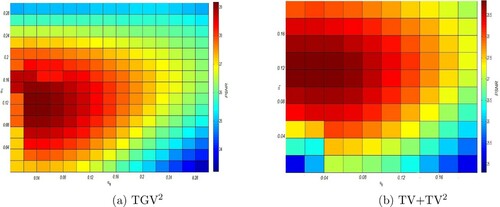
Figure 1. Plot of the PSNR values of the restored image using the TGV and TV+TV${}^2$ approach with respect to the parameters ${\alpha }_0$ and ${\alpha }_1$. We can see that the highest achieved PSNR for the TGV${}^2$ approach is related to the values ${\alpha }_0=0.06$ and ${\alpha }_0=0.04$. For the TV+TV${}^2$ model, the best PSNR corresponds to the values ${\alpha }_0=0.011$ and ${\alpha }_0=0.05$. Note that the original image is the Pirate one corrupted by Gaussian noise of variance 0.3.

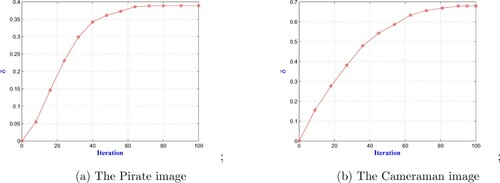
In Figure 2, we show the respective denoised results by different methods. Visually, our method can achieve a reconstruction which is close to one obtained by the TGV method while the other models are outperformed. In the second denoising test, we take the Cameraman image which is a challenging textural image. We consider also the Gaussian noise but with a higher standard deviation $\sigma =0.5$. In order to see the robustness of the proposed method, we present in Figure 3 the restored image with different approaches including the proposed one. Once again, we can observe that visually the proposed method can achieve a better reconstructed result compared to other methods. To see the evolution of the obtained weighting parameter λ, we plot in Figure 4 the values of λ with respect to the iterations for the two above examples. It is then observed that the obtained parameter for the Pirate image is $\lambda =0.39$, while for the Cameraman image the parameter is $\lambda =0.68$.

Figure 2. The obtained denoised image compared to other classical approaches for the (Pirate image), where the noise is considered to be Gaussian of $\sigma =0.3$: (a) Noisy image, (b) ROF model [3], (c) NLM model [51], (d) TV+TV${}^2$ [19] (e) TGV model [36] and (f) Our model.

Figure 3. The obtained denoised image compared to other classical approaches for the (Cameraman image), where the noise is considered to be Gaussian of $\sigma =0.5$: (a) Noisy image, (b) ROF model [3], (c) NLM model [51], (d) TV+TV${}^2$ [19], (e) TGV model [36] and (f) our model.

Figure 4. The computation of the parameter λ with respect to the iteration for the two images Pirate and Cameraman: (a) The Pirate image and (b) The Cameraman image.

For the third and fourth experiments, we change the nature of noise which is considered as an impulse one. For that, we change the fidelity term for the compared methods which is now considered as the L${}^1$ norm since it success in handling the impulse noise (see [2,54,55]). First, we consider the Cameraman image corrupted by an impulse noise with parameter 0.3. Figure 5 shows the obtained denoised image using different approaches with L${}^1$ norm, we can see once again that the proposed method can efficiently reduce the impulse noise without destroying image features, even though the TGV method reduces the noise better than our approach. For the fourth test, we increase the impulse noise level which is taken with parameter 0.5. Figure 6 illustrates the restored image using different regularization methods, we can observe that the proposed approach is visually very sharp compared to the TGV result. Also, we plot in Figure 7 the evolution of the parameter λ with respect to the iterations for the third and fourth examples. It is then observed that the obtained parameter for the Cameraman image is $\lambda =0.81$, while for the Penguin image the parameter is $\lambda =0.90$. Furthermore, to better perform the proposed denoising method over the other methods, a quantitative evaluation is used. In fact, we provide two metrics: PSNR [56] and the mean structure similarity (SSIM) [57]. The PSNR measures signal strength relative to noise in the image while the SSIM metric gives an indication on the quality of the image related to the known characteristics of human visual system. Tables 1 and 2 illustrate the PSNR and SSIM values related to the above simulated tests. We can notice that the proposed model outperforms the compared methods. Moreover, to better compare the quality of reconstructions, we present two tables that indicate the normalized ${\mathit{l}}^{\mathit{2}}$ and ${\mathit{l}}^{\mathit{1}}$-distances between true image and the restored ones. Tables 3 and 4 illustrate the normalized ${\mathit{l}}^{\mathit{2}}$ and ${\mathit{l}}^{\mathit{1}}$-distances values for the four above simulated tests, respectively. Once again, the proposed approach is always with the lower values, which confirm its robustness.

Figure 5. The obtained denoised image compared to other classical approaches for the Cameraman image, where the noise is considered to be impulse one of parameter 0.3: (a) Noisy image, (b) ROF [3], (c) NLM [51], (d) L${}^1$-TV+TV${}^2$ [19], (e) L${}^1$-TGV [36] and (f) Our model.

Figure 6. The obtained denoised image compared to other classical approaches for the (Penguin image), where the noise is considered to be impulse one of parameter 0.5: (a) Noisy image, (b) ROF model [3], (c) NLM model [51], (d) L${}^1$-TV+TV${}^2$ [19], (e) L${}^1$-TGV model [36] and (f) Our model.

Figure 7. The computation of the parameter λ with respect to the iteration for the two images Camerman and Penquin: (a) The Pirate image and (b) The Penguin image.

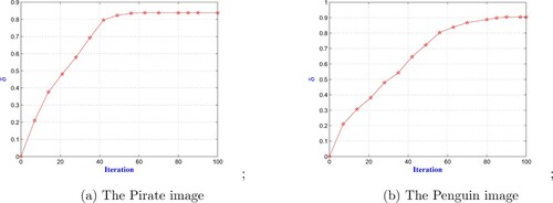
Table 1. The PSNR table.

Image	PSNR
	ROF model [3]	NLM model [51]	TV+TV${}^2$ [19]	TGV model [36]	Our Method
Pirate (Gaussian noise with $\sigma =0.3$)	27.40	28.02	28.88	29.50	$\mathbf{\text{29.88}}$
Cameraman (Gaussian noise with $\sigma =0.5$)	26.90	27.25	28.02	28.28	$\mathbf{\text{29.01}}$
Penguin (impulse noise with parameter 0.3)	23.07	23.80	24.65	$\mathbf{\text{25.11}}$	24.82
Cameraman (impulse noise with parameter 0.5)	26.55	27.03	27.81	28.30	$\mathbf{\text{29.05}}$

Table 2. The SSIM table.

Image	SSIM
	ROF model [3]	NLM model [51]	TV+TV${}^2$ [19]	TGV model [36]	Our Method
Pirate (Gaussian noise with $\sigma =0.3$)	0.886	0.883	0.896	0.902	$\mathbf{\text{0.922}}$
Cameraman (Gaussian noise with $\sigma =0.5$)	0.701	0.707	0.737	0.745	$\mathbf{\text{0.784}}$
Penguin (impulse noise with parameter 0.3)	0.662	0.633	0.698	0.730	$\mathbf{\text{0.738}}$
Cameraman (impulse noise with parameter 0.5)	0.683	0.672	0.763	0.809	$\mathbf{\text{0.814}}$

Table 3. The normalized ${\mathit{l}}^{\mathit{2}}$ distance table.

Image	${\mathit{l}}^{\mathit{1}}$ noise level	$l^2$ distance
		ROF model [3]	NLM model [51]	TV+TV${}^2$ [19]	TGV model [36]	Our Method
Pirate (Gaussian noise with $\sigma =0.3$)	872.4442	351.3230	344.8833	350.1111	341.2931	$\mathbf{\text{307.7933}}$
Cameraman (Gaussian noise with $\sigma =0.5$)	982.3456	522.7418	508.3222	501.6144	498.6666	$\mathbf{\text{473.2997}}$
Penguin (impulse noise with parameter 0.3)	813.1955	612.3734	603.7228	600.6999	587.2444	$\mathbf{\text{576.3333}}$
Cameraman (impulse noise with parameter 0.5)	966.9266	674.6688	669.5133	671.6100	659.0233	$\mathbf{\text{612.9887}}$

Table 4. The normalized ${\mathit{l}}^{\mathit{1}}$ distance table.

Image	${\mathit{l}}^{\mathit{1}}$ noise level	${\mathit{l}}^{\mathit{2}}$ distance
		ROF model [3]	NLM model [51]	TV+TV${}^2$ [19]	TGV model [36]	Our Method
Pirate (Gaussian noise with $\sigma =0.3$)	6.6622e+03	3.3381e+03	2.9363e+03	3.1209e+03	2.7111e+03	$\mathbf{\text{2.5552e+03}}$
Cameraman (Gaussian noise with $\sigma =0.5$)	6.8060e+03	3.4831e+03	3.3332e+03	3.0888e+03	2.9166e+03	$\mathbf{\text{2.7733e+03}}$
Penguin (impulse noise with parameter 0.3)	6.7134e+03	3.5266e+03	3.6001e+03	3.1887e+03	3.30933e+03	$\mathbf{\text{2.9283e+03}}$
Cameraman (impulse noise with parameter 0.5)	7.4333e+03	4.2733e+03	4.5002e+03	4.1666e+03	3.9444e+03	$\mathbf{\text{3.7931e+03}}$

6.2. The space variant case

We now present extensive results to perform the weighted proposed PDE, where the parameter λ is space variant. In fact we are particularly interested to present the results in the space ${\mathcal{U}}_{ad}^2=\{\lambda \in L^2(\mathrm{\Omega }),0<\underset{\_}{\lambda }\le \lambda \le \overline{\lambda }<1\mathrm{a}.\mathrm{e}.x\in \mathrm{\Omega }\mathrm{a}\mathrm{n}\mathrm{d}\parallel \mathrm{\nabla }\lambda {\parallel }_2\le C_0\},$which is the most used space in the literature (especially $\lambda \in H^1\left(\mathrm{\Omega }\right)$ space), see [27–29,58–60], and also the proposed set of admissible filtering weights ${\mathcal{U}}_{ad}^1$ defined by ${\mathcal{U}}_{ad}^1=\{\lambda \in L^1(\mathrm{\Omega }),0<\underset{\_}{\lambda }\le \lambda \le \overline{\lambda }<1\mathrm{a}.\mathrm{e}.x\in \mathrm{\Omega }\mathrm{a}\mathrm{n}\mathrm{d}TV(\lambda )\le C_0\}.$We start by a first experiment where we consider the Lena image which is contaminated by a Gaussian noise with variance $\sigma =0.4$. Then, we use the proposed Algorithm 1 to compute the clean image X and the approximate weighted parameter λ using two different choices of the space of admissible weights λ. The restored image and the spatially variant λ (projected in the image grid: $\lambda \left(X\right)$) using the two sets are displayed in Figure 8.We can observe that the restored image using ${\mathcal{U}}_{ad}^1$ is little sharp compared to the one restored in ${\mathcal{U}}_{ad}^2$, especially near edges. In particular, the approximate λ for the two cases is higher in homogeneous regions and texture, and weaker near edges where the variation is stronger. The next set of experiments is considered to see the behaviour of the proposed weighted PDE with respect to different noise levels using the two admissible spaces. For that, we consider four images which essentially contain combination of large piecewise constant parts and smooth areas. The restored images using the two sets ${\mathcal{U}}_{ad}^1$ and ${\mathcal{U}}_{ad}^2$ are depicted in Figures 9 and 10, respectively. The noisy images are obtained by adding Gaussian noise with variances $\sigma =0.1,0.3,0.4,$ and 0.5, respectively in the same order from the top to the bottom of Figures 9 and 10.From the surface representation of λ, we can detect that λ is smooth enough for ${\mathcal{U}}_{ad}^2$ and piecewise constant for the case of ${\mathcal{U}}_{ad}^1$. For the both cases the shapes of λ are related to the one of the obtained image X, even if for ${\mathcal{U}}_{ad}^1$ the shape of λ is almost the same as the picture. In addition, the same remark as for the previous test remains valid since the values of λ are higher near homogeneous areas.

Figure 8. The restored image and the parameter λ using the two admissible sets of the Lena image: (a) Noisy, (b) X using ${\mathcal{U}}_{ad}^2$, (c) λ using ${\mathcal{U}}_{ad}^2$, (d) X using ${\mathcal{U}}_{ad}^1$ and (e) λ using ${\mathcal{U}}_{ad}^1$.

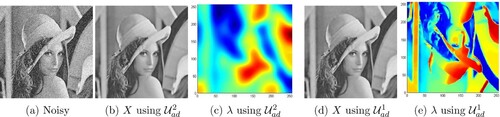
Figure 9. The restored image X and the corresponding weighted parameter λ using the admissible set ${\mathcal{U}}_{ad}^2$. The Baboon image is contaminated by Gaussian noise with $\sigma =0.1$, Penguin image is contaminated by $\sigma =0.3$, Zebra image is contaminated by $\sigma =0.4$, Tiger image is contaminated by $\sigma =0.5$. The used parameters for these tests are: $(k_1,k_2)=(35,89)$, $\sigma =1.3$ and $\rho =2.7$: (a) Noisy, (b) Obtained X, (c) λ and (d) Image of λ.

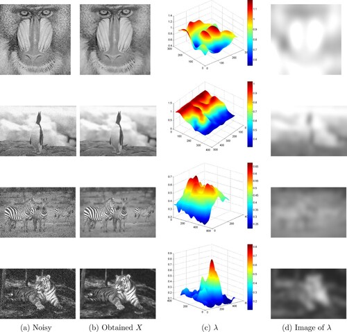
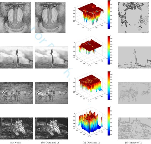
Figure 10. The restored image X and the corresponding weighted parameter λ using the admissible set ${\mathcal{U}}_{ad}^1$. the Baboon image is contaminated by Gaussian noise with $\sigma =0.1$, Penguin image is contaminated by $\sigma =0.3$, Zebra image is contaminated by $\sigma =0.4$, Tiger image is contaminated by $\sigma =0.5$. The used parameters for these tests are: $(k_1,k_2)=(35,80)$, $\sigma =1.7$ and $\rho =2.3$: (a) Noisy, (b) Obtained X, (c) Obtained λ and (d) Image of λ.

The following four tests concern the comparison between the proposed weighted PDE and the spatially dependent regularization parameters for TV image denoising (SDRTV) [27]. For a fair comparison, we consider the same conditions for our approach as for SDRTV one (where $\lambda \in H^1\left(\mathrm{\Omega }\right)$). For that, we set $\lambda \in {\mathcal{U}}_{ad}^2$ for our method and we consider two comparative results. In the two experiments, we treat the denoising problem with brain scan images. The first set consists of image of $256\times 256$ pixels and Gaussian noise with zero mean and variance $\sigma =0.3$. The second one consists of image of $512\times 512$ pixels and Gaussian noise with zero mean and variance $\sigma =0.4$. The used parameters for SDRTV method are $\gamma =40,1013$, $\mu ={10}^{-12},\text{β}={10}^{-10}$ and $h=0.1$. The computed semismooth Newton method, on the whole domain, converges when kmax = 40 iterations. Note that the compared results are done without domain decomposition. For our method, the used parameters are $(k_1,k_2)=(55,40)$, $\sigma =1.8$ and $\rho =2.1$. 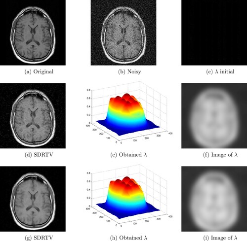The corresponding results are shown in Figures 11 and 12, respectively. By a visual comparison, we can see that the proposed PDE yields significant improvement compared to the SDRTV method. In addition, from the surface representation of λ for the two methods, we can see that λ is continuous and its shape is related to the one of the original image (especially in homogeneous areas).

Figure 11. Comparison between the obtained clean image X and the SDRTV method with the respective computation of the spatially dependent parameter λ of the Head image: (a) Original, (b) Noisy, (c) λ initial, (d) SDRTV, (e) Obtained λ, (f) Image of λ, (g) Proposed PDE, (h) Obtained λ and (i) Image of λ.

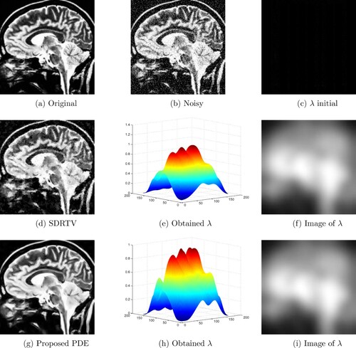
Figure 12. Comparison between the obtained clean image and the SDRTV method and the respective computation of the spatially dependent parameter λ of the Brain image: (a) Original, (b) Noisy, (c) λ initial, (d) SDRTV, (e) Obtained λ, (f) Image of λ, (g) SDRTV, (h) Obtained λ and (i) Image of λ.

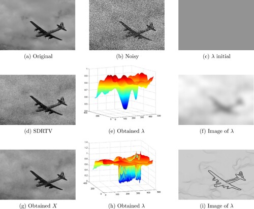
We now consider the proposed admissible set such as $\lambda \in {\mathcal{U}}_{ad}^1$ for our method and we propose two experiment results where we compare our PDE with the SDRTV approach ($\lambda \in H^1\left(\mathrm{\Omega }\right)$). We keep the same parameters as for the previous tests. The noise is considered to be Gaussian one with variances $\sigma =0.3$ and $\sigma =0.5$, respectively. The recovered images are depicted in Figures 13 and 14, respectively. Once again, our method outperforms the SDRTV by a visual comparison. In addition the approximate λ tends to capture more information from the image, which can be interpreted by the less regularity of the proposed set of admissible λ.

Figure 13. Comparison between the obtained clean image X and the SDRTV method with the respective computation of the spatially dependent parameter λ of the Dolphins image: (a) Original, (b) Noisy, (c) λ initial, (d) SDRTV, (e) Obtained λ, (f) Image of λ, (g) Obtained X, (h) Obtained λ and (i) Image of λ.

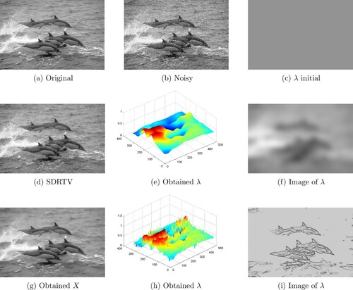
Figure 14. Comparison between the obtained clean image X and the SDRTV method with the respective computation of the spatially-dependent parameter λ of the Plane image: (a) Original, (b) Noisy, (c) λ initial, (d) SDRTV, (e) Obtained λ, (f) Image of λ, (g) Obtained X, (h) Obtained λ and (i) Image of λ.

We end this part by a final example where we give a comparison between the scalar approximate λ, the weighted spatial approximate λ in the respective spaces ${\mathcal{U}}_{ad}^1$ and ${\mathcal{U}}_{ad}^2$. We consider then the image of Fishes, which is a textured challenging example. Then, we add a Gaussian noise with high variance $\sigma =0.5$. The restored image using different λ approximations is presented in Figure 15. In view of the subplots in Figure 15, the obtained spatially variant regularization parameter shares similar patterns to the ones obtained in the previous tests. Particularly, the restored image X using the admissible set ${\mathcal{U}}_{ad}^1$ is visually even better, especially near sharp edges. In addition, the spatially variant result leads to a reduction of the staircasing effect better than the scalar result.

6.3. Robustness of the proposed PDE

In this part, we use four simulated images to perform the choice of the proposed PDE-constrained with the space variant choice of λ. To show the efficiency of the proposed PDE in recovering essential image features, we use some comparisons to other competitive denoising PDEs. In fact, the obtained results are compared to the Fourth-order partial differential equations for image enhancement (FOPDE) [61], Adaptive fourth-order partial differential equation filter for image denoising (AEFD) [62] and the adaptive fourth-order partial differential equation for image denoising (AFOD) [63]. The four tests are done using different levels of Gaussian noise, with $\sigma =30,40,50$ and 60, respectively. In Figure 16, we present the restored image of the four noisy images using the compared enhancement PDEs and our. We can see obviously the robustness of the proposed PDE in avoiding different artefacts compared with the other ones. The used parameters are tuned with respect to the best obtained PSNR. For example the used parameters for the Tiger image are: $\lambda =0.09$, $\mathrm{\Delta }t=0.07$, $\sigma =0.5$, $\mathfrak{K}=0.001$ and 50 iterations for the AEFD approach. $\mu =0.09$, $\mathrm{\Delta }t=0.05$, $k_1=0.05$, $k_2=0.05$, $\gamma ={10}^{-6}$ and 100 iterations for the AFOD approach. $\text{β}={10}^{-4}$, $\mathrm{\Delta }t=0.1$, ${\sigma }_1=0.001$, ${\sigma }_2=0.8$,${\alpha }_1=0.01$, ${\alpha }_2=44$ and 120 iterations for the FOPDE method. Note that the used parameters of our approach are: $(k_1,k_2)=(33,42)$, $\sigma =1.54$, $\rho =3.1$, $\text{β}=1$ and 50 iterations number.

Figure 15. Comparison between the obtained clean image X and the respective computation of the spatially dependent parameter λ for the scalar case and for it two set of admissible values ${\mathcal{U}}_{ad}^1$ and ${\mathcal{U}}_{ad}^2$ for the Fishes image: (a) Original, (b) Noisy, (c) scalar λ, (d) weighted $\lambda \in {\mathcal{U}}_{ad}^2$ and (e) weighted $\lambda \in {\mathcal{U}}_{ad}^1$.

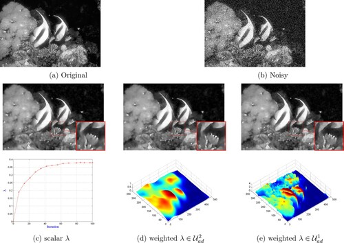
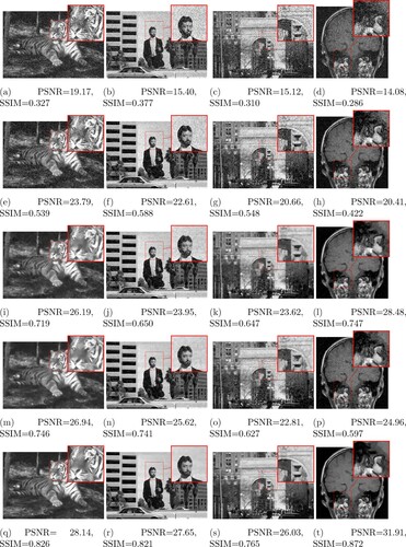
Figure 16. The obtained denoised image compared to other PDE approaches with respect to both quality measures PSNR and SSIM. First row: noisy images. Second row: FOPDE. Third row: AEFD. Fourth row: AFOD. Fifth row: Our approach. (a) PSNR = 19.17, SSIM = 0.327. (b) PSNR = 15.40, SSIM = 0.377. (c) PSNR = 15.12, SSIM = 0.310. (d) PSNR = 14.08, SSIM = 0.286. (e) PSNR = 23.79, SSIM = 0.539. (f) PSNR = 22.61, SSIM = 0.588. (g) PSNR = 20.66, SSIM = 0.548. (h) PSNR = 20.41, SSIM = 0.422, (i) PSNR = 26.19, SSIM = 0.719, (j) PSNR = 23.95, SSIM = 0.650, (k) PSNR = 23.62, SSIM = 0.647. (l) PSNR = 28.48, SSIM = 0.747. (m) PSNR = 26.94, SSIM = 0.746, (n) PSNR = 25.62, SSIM = 0.741, (o) PSNR = 22.81, SSIM = 0.627, (p) PSNR = 24.96, SSIM = 0.597, (q) PSNR = 28.14, SSIM = 0.826, (r) PSNR = 27.65, SSIM = 0.821, (s) PSNR = 26.03, SSIM = 0.765 and (t) PSNR = 31.91, SSIM = 0.872.

7. Conclusion

In this paper, we have introduced a fourth-order PDE-constrained optimization model to treat the denoising task. This PDE is elaborated using a convex combination between two operators controlled by a weighting parameter, which is the solution of the optimal problem. This PDE takes the advantage of the Perona–Malik equation with much regularity and the efficiency of a nonlinear filter to restore tiny and sharp edges. The existence and uniqueness of the proposed PDE-constrained is proved using the Schauder fixed point theorem and the well-posedness of the optimization model is established using the control theory in a suitable space. The results part demonstrates, visually and quantitatively the performance and the contribution of this new PDE over the other denoising approaches. In summary, the proposed approach gives promising analytic strategy for determining an optimal solution for the denoised image and also the parameter λ. As further developments of this method, it may be generalized for other operators and different regularization functional. Another very important generalization of the proposed model is to move from a simple denoising model to more general inverse problems involving linear and nonlinear operators.

Acknowledgments

We are very grateful to the anonymous referees for the remarkable corrections and useful suggestions that have much improved this paper.

Disclosure statement

No potential conflict of interest was reported by the authors.

Appendices

Appendix 1

The next propositions show the differentiability of the solution operator $\mathfrak{S}$. This result leads us to get an expression of the operator ${\mathfrak{S}}^{\mathrm{\prime }}(\lambda {)}^{\ast }$ using the proper adjoint state.

Proposition A.1

Let $\mathfrak{S}:{\mathcal{U}}_{ad}\mapsto L^2\left(\mathrm{\Omega }\right)$ be the solution of Equation (2(2) $\left\{\begin{array}{l}\frac{\mathrm{\partial }X}{\mathrm{\partial }t}+{\mathrm{\nabla }}^2.\left(\lambda D\left(J_{\rho }^{\sigma }\right(\mathrm{\nabla }X\left)\right){\mathrm{\nabla }}^{2}X\right)-\mathrm{\nabla }.\left((1-\lambda )D\left(J_{\rho }^{\sigma }\right(\mathrm{\nabla }X\left)\right)\mathrm{\nabla }X\right)=0\mathrm{i}\mathrm{n}]0,T[\times \mathrm{\Omega },\\ 〈D\left(J_{\rho }^{\sigma }\right(\mathrm{\nabla }X\left)\right)\mathrm{\nabla }X,\nu 〉=0\mathrm{o}\mathrm{n}]0,T[\times \mathrm{\partial }\mathrm{\Omega },\\ X(t,x)=0,\mathrm{o}\mathrm{n}(0,T)\times \mathrm{\partial }\mathrm{\Omega },\\ X(0,x)=X_0\left(x\right),\mathrm{i}\mathrm{n}\mathrm{\Omega },\end{array}\right.$(2) ) at t = T associated to each parameter λ. The operator $\mathfrak{S}$ is Gâteaux differentiable and its derivative at λ, in direction h, is given by the unique solution $X^1$ of the following linearized equation: (A1) $\left\{\begin{array}{l}\frac{\mathrm{\partial }{X}^1}{\mathrm{\partial }t}+{\mathrm{\nabla }}^2.\left(\lambda D\left(J_{\rho }^{\sigma }\right(\mathrm{\nabla }X\left)\right){\mathrm{\nabla }}^2{X}^1\right)-\mathrm{\nabla }.\left((1-\lambda )D\left(J_{\rho }^{\sigma }\right(\mathrm{\nabla }X\left)\right)\mathrm{\nabla }{X}^1\right)+{\mathrm{\nabla }}^2.\left(\lambda D^{\ast }\left(J_{\rho }^{\sigma }\right(\mathrm{\nabla }X\left)\right)X^1{\mathrm{\nabla }}^{2}X\right)\\ -\mathrm{\nabla }.\left((1-\lambda )D^{\ast }\left(J_{\rho }^{\sigma }\right(\mathrm{\nabla }X\left)\right)X^1\mathrm{\nabla }X\right)=-{\mathrm{\nabla }}^2.\left(hD\left(J_{\rho }^{\sigma }\right(\mathrm{\nabla }X\left)\right){\mathrm{\nabla }}^{2}X\right)\\ -\mathrm{\nabla }.\left(hD\left(J_{\rho }^{\sigma }\right(\mathrm{\nabla }X\left)\right)\mathrm{\nabla }X\right)\mathrm{i}\mathrm{n}]0,T[\times \mathrm{\Omega },\\ 〈D\left(J_{\rho }^{\sigma }\right(\mathrm{\nabla }X\left)\right)\mathrm{\nabla }{X}^1〉=0\mathrm{o}\mathrm{n}]0,T[\times \mathrm{\partial }\mathrm{\Omega },\\ X^1(t,x)=0,\mathrm{o}\mathrm{n}(0,T)\times \mathrm{\partial }\mathrm{\Omega },\\ X^1(0,x)=0,\mathrm{i}\mathrm{n}\mathrm{\Omega },\end{array}\right.$(A1) where $D^{\ast }\left(J_{\rho }^{\sigma }\right(\mathrm{\nabla }X\left)\right)=D^{\prime }\left(J_{\rho }^{\sigma }\right(\mathrm{\nabla }X\left)\right)\left(J_{\rho }^{\sigma }\right(\mathrm{\nabla }X){)}^{\prime }$ is the derivative of $D\left(J_{\rho }^{\sigma }\right(\mathrm{\nabla }X\left)\right)$ with respect to state X.

Proof.

We decompose the proof in tree steps:

Step 1 Let $X_{ϵ}$ and X be the unique solutions to (2(2) $\left\{\begin{array}{l}\frac{\mathrm{\partial }X}{\mathrm{\partial }t}+{\mathrm{\nabla }}^2.\left(\lambda D\left(J_{\rho }^{\sigma }\right(\mathrm{\nabla }X\left)\right){\mathrm{\nabla }}^{2}X\right)-\mathrm{\nabla }.\left((1-\lambda )D\left(J_{\rho }^{\sigma }\right(\mathrm{\nabla }X\left)\right)\mathrm{\nabla }X\right)=0\mathrm{i}\mathrm{n}]0,T[\times \mathrm{\Omega },\\ 〈D\left(J_{\rho }^{\sigma }\right(\mathrm{\nabla }X\left)\right)\mathrm{\nabla }X,\nu 〉=0\mathrm{o}\mathrm{n}]0,T[\times \mathrm{\partial }\mathrm{\Omega },\\ X(t,x)=0,\mathrm{o}\mathrm{n}(0,T)\times \mathrm{\partial }\mathrm{\Omega },\\ X(0,x)=X_0\left(x\right),\mathrm{i}\mathrm{n}\mathrm{\Omega },\end{array}\right.$(2) ) corresponding to $\lambda +ϵh$ and λ, respectively for $h\in {\mathcal{U}}_{ad}\subset L^{\mathrm{\infty }}\left(\mathrm{\Omega }\right)\cap BV\left(\mathrm{\Omega }\right)$ and small ϵ. Let's show the priori estimations of the difference of the two solutions $X_{ϵ}$ and X. Taking the difference between the equations of $X_{ϵ}$ and X, we have: (A2) $\begin{array}{rl}& 〈\frac{\mathrm{\partial }{X}_{ϵ}}{\mathrm{\partial }t}-\frac{\mathrm{\partial }X}{\mathrm{\partial }t},\varphi 〉+{\int }_{\mathrm{\Omega }}\lambda (D\left(J_{\rho }^{\sigma }\right(\mathrm{\nabla }{X}_{ϵ}\left)\right){\mathrm{\nabla }}^2{X}_{ϵ}-D\left(J_{\rho }^{\sigma }\right(\mathrm{\nabla }X\left)\right){\mathrm{\nabla }}^{2}X){\mathrm{\nabla }}^2\varphi \mathrm{d}x\\ & +{\int }_{\mathrm{\Omega }}(1-\lambda )(D\left(J_{\rho }^{\sigma }\right(\mathrm{\nabla }{X}_{ϵ}\left)\right)\mathrm{\nabla }{X}_{ϵ}-D\left(J_{\rho }^{\sigma }\right(\mathrm{\nabla }X\left)\right)\mathrm{\nabla }X)\mathrm{\nabla }\varphi \mathrm{d}x\\ & =-ϵ{\int }_{\mathrm{\Omega }}hD\left(J_{\rho }^{\sigma }\right(\mathrm{\nabla }{X}_{ϵ}\left)\right)({\mathrm{\nabla }}^2{X}_{ϵ}{\mathrm{\nabla }}^2\varphi -\mathrm{\nabla }{X}_{ϵ}\mathrm{\nabla }\varphi )\mathrm{d}x,\end{array}$(A2) we can rewrite (A2(A2) $\begin{array}{rl}& 〈\frac{\mathrm{\partial }{X}_{ϵ}}{\mathrm{\partial }t}-\frac{\mathrm{\partial }X}{\mathrm{\partial }t},\varphi 〉+{\int }_{\mathrm{\Omega }}\lambda (D\left(J_{\rho }^{\sigma }\right(\mathrm{\nabla }{X}_{ϵ}\left)\right){\mathrm{\nabla }}^2{X}_{ϵ}-D\left(J_{\rho }^{\sigma }\right(\mathrm{\nabla }X\left)\right){\mathrm{\nabla }}^{2}X){\mathrm{\nabla }}^2\varphi \mathrm{d}x\\ & +{\int }_{\mathrm{\Omega }}(1-\lambda )(D\left(J_{\rho }^{\sigma }\right(\mathrm{\nabla }{X}_{ϵ}\left)\right)\mathrm{\nabla }{X}_{ϵ}-D\left(J_{\rho }^{\sigma }\right(\mathrm{\nabla }X\left)\right)\mathrm{\nabla }X)\mathrm{\nabla }\varphi \mathrm{d}x\\ & =-ϵ{\int }_{\mathrm{\Omega }}hD\left(J_{\rho }^{\sigma }\right(\mathrm{\nabla }{X}_{ϵ}\left)\right)({\mathrm{\nabla }}^2{X}_{ϵ}{\mathrm{\nabla }}^2\varphi -\mathrm{\nabla }{X}_{ϵ}\mathrm{\nabla }\varphi )\mathrm{d}x,\end{array}$(A2) ) as follows: (A3) $\begin{array}{rl}& 〈\frac{\mathrm{\partial }(X_{ϵ}-X)}{\mathrm{\partial }t},\varphi 〉+{\int }_{\mathrm{\Omega }}\lambda D\left(J_{\rho }^{\sigma }\right(\mathrm{\nabla }{X}_{ϵ}\left)\right)({\mathrm{\nabla }}^2(X_{ϵ}-X)){\mathrm{\nabla }}^2\varphi \mathrm{d}x\\ & +{\int }_{\mathrm{\Omega }}(1-\lambda )D\left(J_{\rho }^{\sigma }\right(\mathrm{\nabla }{X}_{ϵ}\left)\right)(\mathrm{\nabla }(X_{ϵ}-X))\mathrm{\nabla }\varphi \mathrm{d}x\\ & +{\int }_{\mathrm{\Omega }}\lambda (D\left(J_{\rho }^{\sigma }\right(\mathrm{\nabla }{X}_{ϵ}\left)\right)-D\left(J_{\rho }^{\sigma }\right(\mathrm{\nabla }X\left)\right)){\mathrm{\nabla }}^{2}X{\mathrm{\nabla }}^2\varphi \\ & +{\int }_{\mathrm{\Omega }}(1-\lambda )(D\left(J_{\rho }^{\sigma }\right(\mathrm{\nabla }{X}_{ϵ}\left)\right)-D\left(J_{\rho }^{\sigma }\right(\mathrm{\nabla }X\left)\right))\mathrm{\nabla }X\mathrm{\nabla }\varphi \mathrm{d}x\\ & =-ϵ{\int }_{\mathrm{\Omega }}hD\left(J_{\rho }^{\sigma }\right(\mathrm{\nabla }{X}_{ϵ}\left)\right)({\mathrm{\nabla }}^2{X}_{ϵ}{\mathrm{\nabla }}^2\varphi -\mathrm{\nabla }{X}_{ϵ}\mathrm{\nabla }\varphi )\mathrm{d}x.\end{array}$(A3) (A4) $\begin{array}{rl}& \parallel {\mathrm{\nabla }}^2(X_{ϵ}-X){\parallel }_{L^2(0,T;L^2(\mathrm{\Omega }\left)\right)}\le Cϵ\parallel h{\parallel }_{L^{\mathrm{\infty }}\left(\mathrm{\Omega }\right)},\end{array}$(A4) (A5) $\begin{array}{rl}& \parallel \mathrm{\nabla }(X_{ϵ}-X){\parallel }_{L^2(0,T;L^2(\mathrm{\Omega }\left)\right)}\le Cϵ\parallel h{\parallel }_{L^{\mathrm{\infty }}\left(\mathrm{\Omega }\right)},\end{array}$(A5) (A6) $\begin{array}{rl}& \parallel X_{ϵ}-X{\parallel }_{L^{\mathrm{\infty }}(0,T;L_0^2(\mathrm{\Omega }\left)\right)}\le Cϵ\parallel h{\parallel }_{L^{\mathrm{\infty }}\left(\mathrm{\Omega }\right)},\end{array}$(A6) and (A7) $\parallel \frac{\mathrm{\partial }(X_{ϵ}-X)}{\mathrm{\partial }t}{\parallel }_{L^2(0,T;H^{-2}(\mathrm{\Omega }\left)\right)}\le Cϵ\parallel h{\parallel }_{L^{\mathrm{\infty }}\left(\mathrm{\Omega }\right)}.$(A7) Step 2 In the second step, we consider the sequence $\{X_{ϵ}^1{\}}_{ϵ>0}$, with $X_{ϵ}^1:=\frac{X_{ϵ}-X}{ϵ}$ and we prove the weak convergence of $X_{ϵ}^1:=\frac{X_{ϵ}-X}{ϵ}$ to $X^1$ solution of Equation (A1(A1) $\left\{\begin{array}{l}\frac{\mathrm{\partial }{X}^1}{\mathrm{\partial }t}+{\mathrm{\nabla }}^2.\left(\lambda D\left(J_{\rho }^{\sigma }\right(\mathrm{\nabla }X\left)\right){\mathrm{\nabla }}^2{X}^1\right)-\mathrm{\nabla }.\left((1-\lambda )D\left(J_{\rho }^{\sigma }\right(\mathrm{\nabla }X\left)\right)\mathrm{\nabla }{X}^1\right)+{\mathrm{\nabla }}^2.\left(\lambda D^{\ast }\left(J_{\rho }^{\sigma }\right(\mathrm{\nabla }X\left)\right)X^1{\mathrm{\nabla }}^{2}X\right)\\ -\mathrm{\nabla }.\left((1-\lambda )D^{\ast }\left(J_{\rho }^{\sigma }\right(\mathrm{\nabla }X\left)\right)X^1\mathrm{\nabla }X\right)=-{\mathrm{\nabla }}^2.\left(hD\left(J_{\rho }^{\sigma }\right(\mathrm{\nabla }X\left)\right){\mathrm{\nabla }}^{2}X\right)\\ -\mathrm{\nabla }.\left(hD\left(J_{\rho }^{\sigma }\right(\mathrm{\nabla }X\left)\right)\mathrm{\nabla }X\right)\mathrm{i}\mathrm{n}]0,T[\times \mathrm{\Omega },\\ 〈D\left(J_{\rho }^{\sigma }\right(\mathrm{\nabla }X\left)\right)\mathrm{\nabla }{X}^1〉=0\mathrm{o}\mathrm{n}]0,T[\times \mathrm{\partial }\mathrm{\Omega },\\ X^1(t,x)=0,\mathrm{o}\mathrm{n}(0,T)\times \mathrm{\partial }\mathrm{\Omega },\\ X^1(0,x)=0,\mathrm{i}\mathrm{n}\mathrm{\Omega },\end{array}\right.$(A1) ).

We have the corresponding Equation (A3(A3) $\begin{array}{rl}& 〈\frac{\mathrm{\partial }(X_{ϵ}-X)}{\mathrm{\partial }t},\varphi 〉+{\int }_{\mathrm{\Omega }}\lambda D\left(J_{\rho }^{\sigma }\right(\mathrm{\nabla }{X}_{ϵ}\left)\right)({\mathrm{\nabla }}^2(X_{ϵ}-X)){\mathrm{\nabla }}^2\varphi \mathrm{d}x\\ & +{\int }_{\mathrm{\Omega }}(1-\lambda )D\left(J_{\rho }^{\sigma }\right(\mathrm{\nabla }{X}_{ϵ}\left)\right)(\mathrm{\nabla }(X_{ϵ}-X))\mathrm{\nabla }\varphi \mathrm{d}x\\ & +{\int }_{\mathrm{\Omega }}\lambda (D\left(J_{\rho }^{\sigma }\right(\mathrm{\nabla }{X}_{ϵ}\left)\right)-D\left(J_{\rho }^{\sigma }\right(\mathrm{\nabla }X\left)\right)){\mathrm{\nabla }}^{2}X{\mathrm{\nabla }}^2\varphi \\ & +{\int }_{\mathrm{\Omega }}(1-\lambda )(D\left(J_{\rho }^{\sigma }\right(\mathrm{\nabla }{X}_{ϵ}\left)\right)-D\left(J_{\rho }^{\sigma }\right(\mathrm{\nabla }X\left)\right))\mathrm{\nabla }X\mathrm{\nabla }\varphi \mathrm{d}x\\ & =-ϵ{\int }_{\mathrm{\Omega }}hD\left(J_{\rho }^{\sigma }\right(\mathrm{\nabla }{X}_{ϵ}\left)\right)({\mathrm{\nabla }}^2{X}_{ϵ}{\mathrm{\nabla }}^2\varphi -\mathrm{\nabla }{X}_{ϵ}\mathrm{\nabla }\varphi )\mathrm{d}x.\end{array}$(A3) ) at $X_{ϵ}^1$ is given as follows: (A8) $\begin{array}{rl}& 〈\frac{\mathrm{\partial }{X}_{ϵ}^1}{\mathrm{\partial }t},\varphi 〉+{\int }_{\mathrm{\Omega }}\lambda D\left(J_{\rho }^{\sigma }\right(\mathrm{\nabla }{X}_{ϵ}\left)\right){\mathrm{\nabla }}^2{X}_{ϵ}^1{\mathrm{\nabla }}^2\varphi \mathrm{d}x+{\int }_{\mathrm{\Omega }}\lambda \frac{D\left(J_{\rho }^{\sigma }\right(\mathrm{\nabla }{X}_{ϵ}\left)\right)-D\left(J_{\rho }^{\sigma }\right(\mathrm{\nabla }X\left)\right)}{ϵ}{\mathrm{\nabla }}^{2}X{\mathrm{\nabla }}^2\varphi \\ & +{\int }_{\mathrm{\Omega }}(1-\lambda )D\left(J_{\rho }^{\sigma }\right(\mathrm{\nabla }{X}_{ϵ}\left)\right)\mathrm{\nabla }{X}_{ϵ}^1\mathrm{\nabla }\varphi \mathrm{d}x+{\int }_{\mathrm{\Omega }}(1-\lambda )\frac{D\left(J_{\rho }^{\sigma }\right(\mathrm{\nabla }{X}_{ϵ}\left)\right)-D\left(J_{\rho }^{\sigma }\right(\mathrm{\nabla }X\left)\right)}{ϵ}\mathrm{\nabla }X\mathrm{\nabla }\varphi \mathrm{d}x\\ & =-{\int }_{\mathrm{\Omega }}hD\left(J_{\rho }^{\sigma }\right(\mathrm{\nabla }{X}_{ϵ}\left)\right)({\mathrm{\nabla }}^2{X}_{ϵ}{\mathrm{\nabla }}^2\varphi -\mathrm{\nabla }{X}_{ϵ}\mathrm{\nabla }\varphi )\mathrm{d}x.\end{array}$(A8) Using the mean value theorem in integral form we get that: (A9) $\begin{array}{rl}& 〈\frac{\mathrm{\partial }{X}_{ϵ}^1}{\mathrm{\partial }t},\varphi 〉+{\int }_{\mathrm{\Omega }}\lambda D\left(J_{\rho }^{\sigma }\right(\mathrm{\nabla }{X}_{ϵ}\left)\right){\mathrm{\nabla }}^2{X}_{ϵ}^1{\mathrm{\nabla }}^2\varphi \mathrm{d}x+{\int }_{\mathrm{\Omega }}\lambda D^{\ast }\left(J_{\rho }^{\sigma }\right(\mathrm{\nabla }{W}_{ϵ}\left)\right)X_{ϵ}^1{\mathrm{\nabla }}^{2}X{\mathrm{\nabla }}^2\varphi \\ & +{\int }_{\mathrm{\Omega }}(1-\lambda )D\left(J_{\rho }^{\sigma }\right(\mathrm{\nabla }{X}_{ϵ}\left)\right)\mathrm{\nabla }{X}_{ϵ}^1\mathrm{\nabla }\varphi \mathrm{d}x+{\int }_{\mathrm{\Omega }}(1-\lambda )D^{\ast }\left(J_{\rho }^{\sigma }\right(\mathrm{\nabla }{W}_{ϵ}\left)\right)X_{ϵ}^1\mathrm{\nabla }X\mathrm{\nabla }\varphi \mathrm{d}x\\ & =-{\int }_{\mathrm{\Omega }}hD\left(J_{\rho }^{\sigma }\right(\mathrm{\nabla }{X}_{ϵ}\left)\right)({\mathrm{\nabla }}^2{X}_{ϵ}{\mathrm{\nabla }}^2\varphi -\mathrm{\nabla }{X}_{ϵ}\mathrm{\nabla }\varphi )\mathrm{d}x.\end{array}$(A9) where $W_{ϵ}=X+{\rho }_{ϵ}(X_{ϵ}-X)$ with $0\le {\rho }_{ϵ}\le 1$.

Using the estimations (A4(A4) $\begin{array}{rl}& \parallel {\mathrm{\nabla }}^2(X_{ϵ}-X){\parallel }_{L^2(0,T;L^2(\mathrm{\Omega }\left)\right)}\le Cϵ\parallel h{\parallel }_{L^{\mathrm{\infty }}\left(\mathrm{\Omega }\right)},\end{array}$(A4) ) and (A7(A7) $\parallel \frac{\mathrm{\partial }(X_{ϵ}-X)}{\mathrm{\partial }t}{\parallel }_{L^2(0,T;H^{-2}(\mathrm{\Omega }\left)\right)}\le Cϵ\parallel h{\parallel }_{L^{\mathrm{\infty }}\left(\mathrm{\Omega }\right)}.$(A7) ) Aubin–Lions and Aubin–Simon lemmas [45–48], we can extract a subsequence denoted again $\left(X_{ϵ}^1\right)$ such that $X_{ϵ}^1\to X^1$ strongly in $L^2(0,T;H_0^1(\mathrm{\Omega }\left)\right)$ and $X_{ϵ}^1\to X^1$ strongly in $L^{\mathrm{\infty }}(0,T;L^2(\mathrm{\Omega }\left)\right)$ as $ϵ\to 0.$ Using the same techniques of convergence we can extract a subsequence denoted again $\left(X_{ϵ}\right)$ such that $X_{ϵ}\to X$ strongly in $L^2(0,T;H_0^1(\mathrm{\Omega }\left)\right)$ and $X_{ϵ}\to X$ strongly in $L^{\mathrm{\infty }}(0,T;L^2(\mathrm{\Omega }\left)\right)$, and thanks to the smoothness of D, and form the definition we have $D^{\ast }$ is continuous. We can pass to the limit in (A9(A9) $\begin{array}{rl}& 〈\frac{\mathrm{\partial }{X}_{ϵ}^1}{\mathrm{\partial }t},\varphi 〉+{\int }_{\mathrm{\Omega }}\lambda D\left(J_{\rho }^{\sigma }\right(\mathrm{\nabla }{X}_{ϵ}\left)\right){\mathrm{\nabla }}^2{X}_{ϵ}^1{\mathrm{\nabla }}^2\varphi \mathrm{d}x+{\int }_{\mathrm{\Omega }}\lambda D^{\ast }\left(J_{\rho }^{\sigma }\right(\mathrm{\nabla }{W}_{ϵ}\left)\right)X_{ϵ}^1{\mathrm{\nabla }}^{2}X{\mathrm{\nabla }}^2\varphi \\ & +{\int }_{\mathrm{\Omega }}(1-\lambda )D\left(J_{\rho }^{\sigma }\right(\mathrm{\nabla }{X}_{ϵ}\left)\right)\mathrm{\nabla }{X}_{ϵ}^1\mathrm{\nabla }\varphi \mathrm{d}x+{\int }_{\mathrm{\Omega }}(1-\lambda )D^{\ast }\left(J_{\rho }^{\sigma }\right(\mathrm{\nabla }{W}_{ϵ}\left)\right)X_{ϵ}^1\mathrm{\nabla }X\mathrm{\nabla }\varphi \mathrm{d}x\\ & =-{\int }_{\mathrm{\Omega }}hD\left(J_{\rho }^{\sigma }\right(\mathrm{\nabla }{X}_{ϵ}\left)\right)({\mathrm{\nabla }}^2{X}_{ϵ}{\mathrm{\nabla }}^2\varphi -\mathrm{\nabla }{X}_{ϵ}\mathrm{\nabla }\varphi )\mathrm{d}x.\end{array}$(A9) ) to obtain the following formula: (A10) $\begin{array}{rl}& 〈\frac{\mathrm{\partial }{X}^1}{\mathrm{\partial }t},\varphi 〉+{\int }_{\mathrm{\Omega }}\lambda D\left(J_{\rho }^{\sigma }\right(\mathrm{\nabla }X\left)\right){\mathrm{\nabla }}^2{X}^1{\mathrm{\nabla }}^2\varphi \mathrm{d}x+{\int }_{\mathrm{\Omega }}\lambda D^{\ast }\left(J_{\rho }^{\sigma }\right(\mathrm{\nabla }X)X^1{\mathrm{\nabla }}^{2}X{\mathrm{\nabla }}^2\varphi \\ & +{\int }_{\mathrm{\Omega }}(1-\lambda )D\left(J_{\rho }^{\sigma }\right(\mathrm{\nabla }X\left)\right)\mathrm{\nabla }{X}^1\mathrm{\nabla }\varphi \mathrm{d}x+{\int }_{\mathrm{\Omega }}(1-\lambda )D^{\ast }\left(J_{\rho }^{\sigma }\right(\mathrm{\nabla }X)X^1\mathrm{\nabla }X\mathrm{\nabla }\varphi \mathrm{d}x\\ & =-{\int }_{\mathrm{\Omega }}hD\left(J_{\rho }^{\sigma }\right(\mathrm{\nabla }X\left)\right)({\mathrm{\nabla }}^{2}X{\mathrm{\nabla }}^2\varphi -\mathrm{\nabla }X\mathrm{\nabla }\varphi )\mathrm{d}x.\end{array}$(A10) Consequently, $X^1$ corresponds to the solution of the linearised equation (A1(A1) $\left\{\begin{array}{l}\frac{\mathrm{\partial }{X}^1}{\mathrm{\partial }t}+{\mathrm{\nabla }}^2.\left(\lambda D\left(J_{\rho }^{\sigma }\right(\mathrm{\nabla }X\left)\right){\mathrm{\nabla }}^2{X}^1\right)-\mathrm{\nabla }.\left((1-\lambda )D\left(J_{\rho }^{\sigma }\right(\mathrm{\nabla }X\left)\right)\mathrm{\nabla }{X}^1\right)+{\mathrm{\nabla }}^2.\left(\lambda D^{\ast }\left(J_{\rho }^{\sigma }\right(\mathrm{\nabla }X\left)\right)X^1{\mathrm{\nabla }}^{2}X\right)\\ -\mathrm{\nabla }.\left((1-\lambda )D^{\ast }\left(J_{\rho }^{\sigma }\right(\mathrm{\nabla }X\left)\right)X^1\mathrm{\nabla }X\right)=-{\mathrm{\nabla }}^2.\left(hD\left(J_{\rho }^{\sigma }\right(\mathrm{\nabla }X\left)\right){\mathrm{\nabla }}^{2}X\right)\\ -\mathrm{\nabla }.\left(hD\left(J_{\rho }^{\sigma }\right(\mathrm{\nabla }X\left)\right)\mathrm{\nabla }X\right)\mathrm{i}\mathrm{n}]0,T[\times \mathrm{\Omega },\\ 〈D\left(J_{\rho }^{\sigma }\right(\mathrm{\nabla }X\left)\right)\mathrm{\nabla }{X}^1〉=0\mathrm{o}\mathrm{n}]0,T[\times \mathrm{\partial }\mathrm{\Omega },\\ X^1(t,x)=0,\mathrm{o}\mathrm{n}(0,T)\times \mathrm{\partial }\mathrm{\Omega },\\ X^1(0,x)=0,\mathrm{i}\mathrm{n}\mathrm{\Omega },\end{array}\right.$(A1) ) with (A11) $\begin{array}{rl}& \parallel {\mathrm{\nabla }}^2{X}^1{\parallel }_{L^2(0,T;L^2(\mathrm{\Omega }\left)\right)}\le C\parallel h{\parallel }_{L^{\mathrm{\infty }}\left(\mathrm{\Omega }\right)},\end{array}$(A11) (A12) $\begin{array}{rl}& \parallel \mathrm{\nabla }{X}^1{\parallel }_{L^2(0,T;L^2(\mathrm{\Omega }\left)\right)}\le C\parallel h{\parallel }_{L^{\mathrm{\infty }}\left(\mathrm{\Omega }\right)},\end{array}$(A12) (A13) $\begin{array}{rl}& \parallel X^1{\parallel }_{L^{\mathrm{\infty }}(0,T;L_0^2(\mathrm{\Omega }\left)\right)}\le C\parallel h{\parallel }_{L^{\mathrm{\infty }}\left(\mathrm{\Omega }\right)},\end{array}$(A13) and (A14) $\parallel \frac{\mathrm{\partial }{X}^1}{\mathrm{\partial }t}{\parallel }_{L^2(0,T;H^{-2}(\mathrm{\Omega }\left)\right)}\le C\parallel h{\parallel }_{L^{\mathrm{\infty }}\left(\mathrm{\Omega }\right)}.$(A14) Step 3 Now, we will prove that the sequence $X_{ϵ}^1$ converges strongly in $L^2(0,T;H_0^2(\mathrm{\Omega }\left)\right)$ to $X^1$. As a consequence of the previous step, it suffices to prove that: ${\mathrm{\nabla }}^2{X}_{ϵ}^1\to {\mathrm{\nabla }}^2{X}^1\mathrm{i}\mathrm{n}\left(L^2\right(\mathrm{\Omega }){)}^2$Let consider two Matrix: $M_{ϵ}=(\lambda +ϵh)D\left(J_{\rho }^{\sigma }\right(\mathrm{\nabla }{X}_{ϵ}\left)\right)\mathrm{a}\mathrm{n}\mathrm{d}M=D\left(J_{\rho }^{\sigma }\right(\mathrm{\nabla }X\left)\right)$$M_{ϵ}$ and M are symmetric and positive definite. Using Cholesky decomposition we obtain lower triangular matrices $L_{ϵ}$ and L such that $M_{ϵ}=L_{ϵ}{L}_{ϵ}^T\mathrm{a}\mathrm{n}\mathrm{d}M=L{L}^T.$Applying the same convergence as in step 2 in the weak formulation (A9(A9) $\begin{array}{rl}& 〈\frac{\mathrm{\partial }{X}_{ϵ}^1}{\mathrm{\partial }t},\varphi 〉+{\int }_{\mathrm{\Omega }}\lambda D\left(J_{\rho }^{\sigma }\right(\mathrm{\nabla }{X}_{ϵ}\left)\right){\mathrm{\nabla }}^2{X}_{ϵ}^1{\mathrm{\nabla }}^2\varphi \mathrm{d}x+{\int }_{\mathrm{\Omega }}\lambda D^{\ast }\left(J_{\rho }^{\sigma }\right(\mathrm{\nabla }{W}_{ϵ}\left)\right)X_{ϵ}^1{\mathrm{\nabla }}^{2}X{\mathrm{\nabla }}^2\varphi \\ & +{\int }_{\mathrm{\Omega }}(1-\lambda )D\left(J_{\rho }^{\sigma }\right(\mathrm{\nabla }{X}_{ϵ}\left)\right)\mathrm{\nabla }{X}_{ϵ}^1\mathrm{\nabla }\varphi \mathrm{d}x+{\int }_{\mathrm{\Omega }}(1-\lambda )D^{\ast }\left(J_{\rho }^{\sigma }\right(\mathrm{\nabla }{W}_{ϵ}\left)\right)X_{ϵ}^1\mathrm{\nabla }X\mathrm{\nabla }\varphi \mathrm{d}x\\ & =-{\int }_{\mathrm{\Omega }}hD\left(J_{\rho }^{\sigma }\right(\mathrm{\nabla }{X}_{ϵ}\left)\right)({\mathrm{\nabla }}^2{X}_{ϵ}{\mathrm{\nabla }}^2\varphi -\mathrm{\nabla }{X}_{ϵ}\mathrm{\nabla }\varphi )\mathrm{d}x.\end{array}$(A9) ) with the function test is $X_{ϵ}^1$ and integrating by parts we obtain (A15) $\begin{array}{rl}& \underset{ϵ\to 0}{lim}{\int }_0^T{\int }_{\mathrm{\Omega }}{M}_{ϵ}{\mathrm{\nabla }}^2{X}_{ϵ}^1{\mathrm{\nabla }}^2{X}_{ϵ}^1\mathrm{d}x\mathrm{d}t=-\frac{1}{2}\parallel X^1(.,T){\parallel }_{L^2\left(\mathrm{\Omega }\right)}^2\\ & -{\int }_0^T{\int }_{\mathrm{\Omega }}(1-\lambda )D^{\ast }\left(J_{\rho }^{\sigma }\right(\mathrm{\nabla }X\left)\right)X^1{\mathrm{\nabla }}^{2}X{\mathrm{\nabla }}^2{X}^1\mathrm{d}x\mathrm{d}t\\ & -{\int }_0^T{\int }_{\mathrm{\Omega }}(1-\lambda )D\left(J_{\rho }^{\sigma }\right(\mathrm{\nabla }X\left)\right)\mathrm{\nabla }{X}^1\mathrm{\nabla }{X}^1\mathrm{d}x\mathrm{d}t-{\int }_0^T{\int }_{\mathrm{\Omega }}(1-\lambda )D^{\ast }\left(J_{\rho }^{\sigma }\right(\mathrm{\nabla }X\left)\right)X^1\mathrm{\nabla }X\mathrm{\nabla }{X}^1\mathrm{d}x\mathrm{d}t\\ & +{\int }_0^T{\int }_{\mathrm{\Omega }}hD\left(J_{\rho }^{\sigma }\right(\mathrm{\nabla }X\left)\right)({\mathrm{\nabla }}^{2}X{\mathrm{\nabla }}^2{X}^1-\mathrm{\nabla }X\mathrm{\nabla }{X}^1)\mathrm{d}x\mathrm{d}t={\int }_0^T{\int }_{\mathrm{\Omega }}M{\mathrm{\nabla }}^2{X}^1{\mathrm{\nabla }}^2{X}^1\mathrm{d}x\mathrm{d}t\\ & {\int }_0^T{\int }_{\mathrm{\Omega }}{M}_{ϵ}{\mathrm{\nabla }}^2{X}_{ϵ}^1{\mathrm{\nabla }}^2{X}_{ϵ}^1\mathrm{d}x\mathrm{d}t\to {\int }_0^T{\int }_{\mathrm{\Omega }}M{\mathrm{\nabla }}^2{X}^1{\mathrm{\nabla }}^2{X}^1\mathrm{d}x\mathrm{d}t\mathrm{a}\mathrm{s}ϵ\to 0,\end{array}$(A15) Using the above equation and (A10(A10) $\begin{array}{rl}& 〈\frac{\mathrm{\partial }{X}^1}{\mathrm{\partial }t},\varphi 〉+{\int }_{\mathrm{\Omega }}\lambda D\left(J_{\rho }^{\sigma }\right(\mathrm{\nabla }X\left)\right){\mathrm{\nabla }}^2{X}^1{\mathrm{\nabla }}^2\varphi \mathrm{d}x+{\int }_{\mathrm{\Omega }}\lambda D^{\ast }\left(J_{\rho }^{\sigma }\right(\mathrm{\nabla }X)X^1{\mathrm{\nabla }}^{2}X{\mathrm{\nabla }}^2\varphi \\ & +{\int }_{\mathrm{\Omega }}(1-\lambda )D\left(J_{\rho }^{\sigma }\right(\mathrm{\nabla }X\left)\right)\mathrm{\nabla }{X}^1\mathrm{\nabla }\varphi \mathrm{d}x+{\int }_{\mathrm{\Omega }}(1-\lambda )D^{\ast }\left(J_{\rho }^{\sigma }\right(\mathrm{\nabla }X)X^1\mathrm{\nabla }X\mathrm{\nabla }\varphi \mathrm{d}x\\ & =-{\int }_{\mathrm{\Omega }}hD\left(J_{\rho }^{\sigma }\right(\mathrm{\nabla }X\left)\right)({\mathrm{\nabla }}^{2}X{\mathrm{\nabla }}^2\varphi -\mathrm{\nabla }X\mathrm{\nabla }\varphi )\mathrm{d}x.\end{array}$(A10) ), we prove by the same argumentation as in ([64], Theorem 3.1, Step 3) that which implies that ${\mathrm{\nabla }}^2{X}_{ϵ}^1\to {\mathrm{\nabla }}^2{X}^1\mathrm{i}\mathrm{n}{L}^2(0,T;L^2(\mathrm{\Omega }\left)\right).$

We can find by using the same techniques that $\frac{\mathrm{\partial }{X}_{ϵ}^1}{\mathrm{\partial }t}\to \frac{\mathrm{\partial }{X}^1}{\mathrm{\partial }t}\mathrm{i}\mathrm{n}{L}^2(0,T;H^{-2}(\mathrm{\Omega }\left)\right).$ This complete the proof.

Based on the differentiability properties of the solution operator, we give in next proposition the expression of adjoint derivative operator ${\mathfrak{S}}^{\mathrm{\prime }}\left(\lambda {)}^{\ast }\right(.)$.

Proposition A.2

We have: (A16) ${\mathfrak{S}}^{\mathrm{\prime }}(\lambda {)}^{\ast }W=-{\int }_{}^{T}D(J_{\rho }^{\sigma }\left(\mathrm{\nabla }X\right)){\mathrm{\nabla }}^{2}X{\mathrm{\nabla }}^{2}P\mathrm{d}t+{\int }_0^{T}D(J_{\rho }^{\sigma }\left(\mathrm{\nabla }X\right))\mathrm{\nabla }X\mathrm{\nabla }P\mathrm{d}t,$(A16) where P is the solution of the following adjoint problem: (A17) $\left\{\begin{array}{l}-\frac{\mathrm{\partial }P}{\mathrm{\partial }t}+{\mathrm{\nabla }}^2.\left(\lambda D\left(J_{\rho }^{\sigma }\right(\mathrm{\nabla }X\left)\right){\mathrm{\nabla }}^{2}P\right)-\mathrm{\nabla }.\left((1-\lambda )D\left(J_{\rho }^{\sigma }\right(\mathrm{\nabla }X\left)\right)\mathrm{\nabla }P\right)\\ +\lambda D^{\ast }\left(J_{\rho }^{\sigma }\right(\mathrm{\nabla }X\left)\right){\mathrm{\nabla }}^{2}X{\mathrm{\nabla }}^{2}P+(1-\lambda )D^{\ast }\left(J_{\rho }^{\sigma }\right(\mathrm{\nabla }X\left)\right)\mathrm{\nabla }X\mathrm{\nabla }P=0\mathit{i}\mathit{n}\mathit{]}\mathit{0}\mathit{,}\mathit{T}\mathit{[}\times \mathit{\Omega }\mathit{,}\\ 〈D\left(J_{\rho }^{\sigma }\right(\mathrm{\nabla }X\left)\right)\mathrm{\nabla }P,\nu 〉=0\mathit{o}\mathit{n}\mathit{]}\mathit{0}\mathit{,}\mathit{T}\mathit{[}\times \mathrm{\partial }\mathit{\Omega }\mathit{,}\\ P(t,x)=0,\mathrm{o}\mathrm{n},(0,T)\times \mathrm{\partial }\mathrm{\Omega },\\ P(T,x)=W\left(x\right),\mathrm{i}\mathrm{n}\mathrm{\Omega },\end{array}\right.$(A17)

Proof.

To prove the result (74(74) ${\mathfrak{S}}^{\mathrm{\prime }}(\lambda {)}^{\ast }W=-{\int }_0^{T}D(J_{\rho }^{\sigma }\left(\mathrm{\nabla }X\right)){\mathrm{\nabla }}^{2}X{\mathrm{\nabla }}^{2}P\mathrm{d}t+{\int }_0^{T}D(J_{\rho }^{\sigma }\left(\mathrm{\nabla }X\right))\mathrm{\nabla }X\mathrm{\nabla }P\mathrm{d}t,$(74) ), we take $\varphi \in L^2(0,T;H_0^2(\mathrm{\Omega }\left)\right)$ as function test in the variational form of system (A1(A1) $\left\{\begin{array}{l}\frac{\mathrm{\partial }{X}^1}{\mathrm{\partial }t}+{\mathrm{\nabla }}^2.\left(\lambda D\left(J_{\rho }^{\sigma }\right(\mathrm{\nabla }X\left)\right){\mathrm{\nabla }}^2{X}^1\right)-\mathrm{\nabla }.\left((1-\lambda )D\left(J_{\rho }^{\sigma }\right(\mathrm{\nabla }X\left)\right)\mathrm{\nabla }{X}^1\right)+{\mathrm{\nabla }}^2.\left(\lambda D^{\ast }\left(J_{\rho }^{\sigma }\right(\mathrm{\nabla }X\left)\right)X^1{\mathrm{\nabla }}^{2}X\right)\\ -\mathrm{\nabla }.\left((1-\lambda )D^{\ast }\left(J_{\rho }^{\sigma }\right(\mathrm{\nabla }X\left)\right)X^1\mathrm{\nabla }X\right)=-{\mathrm{\nabla }}^2.\left(hD\left(J_{\rho }^{\sigma }\right(\mathrm{\nabla }X\left)\right){\mathrm{\nabla }}^{2}X\right)\\ -\mathrm{\nabla }.\left(hD\left(J_{\rho }^{\sigma }\right(\mathrm{\nabla }X\left)\right)\mathrm{\nabla }X\right)\mathrm{i}\mathrm{n}]0,T[\times \mathrm{\Omega },\\ 〈D\left(J_{\rho }^{\sigma }\right(\mathrm{\nabla }X\left)\right)\mathrm{\nabla }{X}^1〉=0\mathrm{o}\mathrm{n}]0,T[\times \mathrm{\partial }\mathrm{\Omega },\\ X^1(t,x)=0,\mathrm{o}\mathrm{n}(0,T)\times \mathrm{\partial }\mathrm{\Omega },\\ X^1(0,x)=0,\mathrm{i}\mathrm{n}\mathrm{\Omega },\end{array}\right.$(A1) ) and (75(75) $\left\{\begin{array}{l}-\frac{\mathrm{\partial }P}{\mathrm{\partial }t}+{\mathrm{\nabla }}^2.\left(\lambda D\left(J_{\rho }^{\sigma }\right(\mathrm{\nabla }X\left)\right){\mathrm{\nabla }}^{2}P\right)-\mathrm{\nabla }.\left((1-\lambda )D\left(J_{\rho }^{\sigma }\right(\mathrm{\nabla }X\left)\right)\mathrm{\nabla }P\right)\\ +\lambda D^{\ast }\left(J_{\rho }^{\sigma }\right(\mathrm{\nabla }X\left)\right){\mathrm{\nabla }}^{2}X{\mathrm{\nabla }}^{2}P+(1-\lambda )D^{\ast }\left(J_{\rho }^{\sigma }\right(\mathrm{\nabla }X\left)\right)\mathrm{\nabla }X\mathrm{\nabla }P=0\mathrm{i}\mathrm{n}]0,T[\times \mathrm{\Omega },\\ 〈D\left(J_{\rho }^{\sigma }\right(\mathrm{\nabla }X\left)\right)\mathrm{\nabla }P,\nu 〉=0\mathrm{o}\mathrm{n}]0,T[\times \mathrm{\partial }\mathrm{\Omega },\\ P(t,x)=0,\mathrm{o}\mathrm{n}(0,T)\times \mathrm{\partial }\mathrm{\Omega },\\ P(T,x)=W\left(x\right),\mathrm{i}\mathrm{n}\mathrm{\Omega },\end{array}\right.$(75) ), which give: (A18) $\begin{array}{rl}& {\int }_0^T〈\frac{\mathrm{\partial }{X}^1}{\mathrm{\partial }t},\varphi 〉+{\int }_0^T{\int }_{\mathrm{\Omega }}\lambda D\left(J_{\rho }^{\sigma }\right(\mathrm{\nabla }X\left)\right){\mathrm{\nabla }}^2{X}^1{\mathrm{\nabla }}^2\varphi +{\int }_0^T{\int }_{\mathrm{\Omega }}(1-\lambda )D\left(J_{\rho }^{\sigma }\right(\mathrm{\nabla }X\left)\right)\mathrm{\nabla }{X}^1\mathrm{\nabla }\varphi \\ & +{\int }_0^T{\int }_{\mathrm{\Omega }}\lambda D^{\ast }\left(J_{\rho }^{\sigma }\right(\mathrm{\nabla }X\left)\right)X^1{\mathrm{\nabla }}^{2}X{\mathrm{\nabla }}^2\varphi +{\int }_0^T{\int }_{\mathrm{\Omega }}(1-\lambda )D^{\ast }\left(J_{\rho }^{\sigma }\right(\mathrm{\nabla }X\left)\right)X^1\mathrm{\nabla }X\mathrm{\nabla }\varphi \\ & =-{\int }_0^T{\int }_{\mathrm{\Omega }}hD\left(J_{\rho }^{\sigma }\right(\mathrm{\nabla }X\left)\right){\mathrm{\nabla }}^{2}X\mathrm{\nabla }\varphi +{\int }_0^T{\int }_{\mathrm{\Omega }}hD\left(J_{\rho }^{\sigma }\right(\mathrm{\nabla }X\left)\right)\mathrm{\nabla }X\mathrm{\nabla }\varphi \end{array}$(A18) and (A19) $\begin{array}{rl}& {\int }_0^T〈-\frac{\mathrm{\partial }P}{\mathrm{\partial }t},\varphi 〉+{\int }_0^T{\int }_{\mathrm{\Omega }}\lambda D\left(J_{\rho }^{\sigma }\right(\mathrm{\nabla }X\left)\right){\mathrm{\nabla }}^{2}P{\mathrm{\nabla }}^2\varphi +{\int }_{\mathrm{\Omega }}(1-\lambda )D\left(J_{\rho }^{\sigma }\right(\mathrm{\nabla }X\left)\right)\mathrm{\nabla }P\mathrm{\nabla }\varphi \\ & +{\int }_0^T{\int }_{\mathrm{\Omega }}\lambda D^{\ast }\left(J_{\rho }^{\sigma }\right(\mathrm{\nabla }X\left)\right){\mathrm{\nabla }}^{2}X{\mathrm{\nabla }}^{2}P\varphi +{\int }_0^T{\int }_{\mathrm{\Omega }}(1-\lambda )D^{\ast }\left(J_{\rho }^{\sigma }\right(\mathrm{\nabla }X\left)\right)\mathrm{\nabla }X\mathrm{\nabla }P\varphi =0\end{array}$(A19) Taking $\varphi =P$ in Equation (A18(A18) $\begin{array}{rl}& {\int }_0^T〈\frac{\mathrm{\partial }{X}^1}{\mathrm{\partial }t},\varphi 〉+{\int }_0^T{\int }_{\mathrm{\Omega }}\lambda D\left(J_{\rho }^{\sigma }\right(\mathrm{\nabla }X\left)\right){\mathrm{\nabla }}^2{X}^1{\mathrm{\nabla }}^2\varphi +{\int }_0^T{\int }_{\mathrm{\Omega }}(1-\lambda )D\left(J_{\rho }^{\sigma }\right(\mathrm{\nabla }X\left)\right)\mathrm{\nabla }{X}^1\mathrm{\nabla }\varphi \\ & +{\int }_0^T{\int }_{\mathrm{\Omega }}\lambda D^{\ast }\left(J_{\rho }^{\sigma }\right(\mathrm{\nabla }X\left)\right)X^1{\mathrm{\nabla }}^{2}X{\mathrm{\nabla }}^2\varphi +{\int }_0^T{\int }_{\mathrm{\Omega }}(1-\lambda )D^{\ast }\left(J_{\rho }^{\sigma }\right(\mathrm{\nabla }X\left)\right)X^1\mathrm{\nabla }X\mathrm{\nabla }\varphi \\ & =-{\int }_0^T{\int }_{\mathrm{\Omega }}hD\left(J_{\rho }^{\sigma }\right(\mathrm{\nabla }X\left)\right){\mathrm{\nabla }}^{2}X\mathrm{\nabla }\varphi +{\int }_0^T{\int }_{\mathrm{\Omega }}hD\left(J_{\rho }^{\sigma }\right(\mathrm{\nabla }X\left)\right)\mathrm{\nabla }X\mathrm{\nabla }\varphi \end{array}$(A18) ) and $\varphi =X^1$ in Equation (A19(A19) $\begin{array}{rl}& {\int }_0^T〈-\frac{\mathrm{\partial }P}{\mathrm{\partial }t},\varphi 〉+{\int }_0^T{\int }_{\mathrm{\Omega }}\lambda D\left(J_{\rho }^{\sigma }\right(\mathrm{\nabla }X\left)\right){\mathrm{\nabla }}^{2}P{\mathrm{\nabla }}^2\varphi +{\int }_{\mathrm{\Omega }}(1-\lambda )D\left(J_{\rho }^{\sigma }\right(\mathrm{\nabla }X\left)\right)\mathrm{\nabla }P\mathrm{\nabla }\varphi \\ & +{\int }_0^T{\int }_{\mathrm{\Omega }}\lambda D^{\ast }\left(J_{\rho }^{\sigma }\right(\mathrm{\nabla }X\left)\right){\mathrm{\nabla }}^{2}X{\mathrm{\nabla }}^{2}P\varphi +{\int }_0^T{\int }_{\mathrm{\Omega }}(1-\lambda )D^{\ast }\left(J_{\rho }^{\sigma }\right(\mathrm{\nabla }X\left)\right)\mathrm{\nabla }X\mathrm{\nabla }P\varphi =0\end{array}$(A19) ) and use the formula ${\int }_0^T〈\frac{\mathrm{\partial }{X}^1}{\mathrm{\partial }t},P〉={\int }_0^T〈-\frac{\mathrm{\partial }P}{\mathrm{\partial }t},X^1〉+{\int }_{\mathrm{\Omega }}{X}^1(x,T)P(x,T)\mathrm{d}x,$it immediately shows that ${\int }_{\mathrm{\Omega }}{X}^1(x,T)P(x,T)\mathrm{d}x=-{\int }_0^T{\int }_{\mathrm{\Omega }}hD\left(J_{\rho }^{\sigma }\right(\mathrm{\nabla }X\left)\right){\mathrm{\nabla }}^{2}X{\mathrm{\nabla }}^{2}P\mathrm{d}t+{\int }_0^T{\int }_{\mathrm{\Omega }}hD\left(J_{\rho }^{\sigma }\right(\mathrm{\nabla }X\left)\right)\mathrm{\nabla }X\mathrm{\nabla }P\mathrm{d}x\mathrm{d}t$To finish this the proof, we use the proposed notation $X^1\left(T\right)=K^{\prime }\left(\lambda \right)h={\mathfrak{S}}^{\prime }\left(\lambda \right)h$ and $P\left(T\right)=W$ then, we have $〈{\mathfrak{S}}^{\prime }\left(\lambda \right)h,W〉=-〈{\int }_0^T(D\left(J_{\rho }^{\sigma }\right(\mathrm{\nabla }X\left)\right){\mathrm{\nabla }}^{2}X{\mathrm{\nabla }}^{2}P-D\left(J_{\rho }^{\sigma }\right(\mathrm{\nabla }X\left)\right)\mathrm{\nabla }X\mathrm{\nabla }P)\mathrm{d}t,h〉.$which completes the proof.

Appendix 2

We introduce the functional space $H_0^2\left(\mathrm{\Omega }\right),$ which is defined as the closure of $C_c^{\mathrm{\infty }}\left(\mathrm{\Omega }\right)$ in $H^2\left(\mathrm{\Omega }\right).$ Thanks to the Lipschitz regularity of the boundary, which leads to the definition $H_0^2\left(\mathrm{\Omega }\right)=\left\{u\in H_0^1\left(\mathrm{\Omega }\right)\cap H^2\left(\mathrm{\Omega }\right)\text{ such that }\mathrm{\nabla }u\cdot n=0\text{ a.e. on }\mathrm{\partial }\mathrm{\Omega }\right\}.$The space $H_0^2\left(\mathrm{\Omega }\right)$ equipped by the norm $\parallel \mathrm{\Delta }u{\parallel }_{L^2\left(\mathrm{\Omega }\right)},$ which is equivalent to the $\parallel u{\parallel }_{H^2\left(\mathrm{\Omega }\right)}$ for every $u\in H_0^2\left(\mathrm{\Omega }\right)$ (see [65,66]). Indeed, the Poincaré inequality $\mathrm{\forall }u\in H_0^1\left(\mathrm{\Omega }\right),\parallel u{\parallel }_{L^2\left(\mathrm{\Omega }\right)}\le C\parallel \mathrm{\nabla }u{\parallel }_{L^2(\mathrm{\Omega }{)}^2}$and $\mathrm{\forall }u\in H_0^2\left(\mathrm{\Omega }\right),-{\int }_{\mathrm{\Omega }}u\mathrm{\Delta }u\mathrm{d}x={\int }_{\mathrm{\Omega }}\mathrm{\nabla }u\mathrm{\nabla }u\mathrm{d}x,$leads to $\mathrm{\forall }u\in H_0^2\left(\mathrm{\Omega }\right),\parallel \mathrm{\nabla }u{\parallel }_{L^2(\mathrm{\Omega }{)}^2}\le C\parallel \mathrm{\Delta }u{\parallel }_{L^2\left(\mathrm{\Omega }\right)}.$Besides, the following equality which is an immediate consequence of two integrations by parts $\mathrm{\forall }\varphi \in C_c^{\mathrm{\infty }}\left(\mathrm{\Omega }\right),{\int }_{\mathrm{\Omega }}(\mathrm{\Delta }\varphi {)}^2\mathrm{d}x=\sum _{i=1}^2\sum _{j=1}^2{\int }_{\mathrm{\Omega }}\frac{{\mathrm{\partial }}^2\varphi }{{\mathrm{\partial }}^2{x}_i}\frac{{\mathrm{\partial }}^2\varphi }{{\mathrm{\partial }}^2{x}_j}\mathrm{d}x=\sum _{i=1}^2\sum _{j=1}^2{\int }_{\mathrm{\Omega }}(\frac{{\mathrm{\partial }}^2\varphi }{\mathrm{\partial }{x}_i\mathrm{\partial }{x}_j}{)}^2\mathrm{d}x.$Now we give the definition of some useful operators. We have ${\mathrm{d}\mathrm{i}\mathrm{v}}^2\left(A\right)=\frac{{\mathrm{\partial }}^2{A}_{12}}{\mathrm{\partial }{x}_1\mathrm{\partial }{x}_2}+\frac{{\mathrm{\partial }}^2{A}_{21}}{\mathrm{\partial }{x}_2\mathrm{\partial }{x}_1}+\sum _{i=1}^2\frac{{\mathrm{\partial }}^2{A}_{ii}}{{\mathrm{\partial }}^2{x}_i},\mathrm{\forall }A\in C_c^{\mathrm{\infty }}(\mathrm{\Omega },{\mathbb{R}}^{2\times 2})$and ${\mathrm{\nabla }}^{2}f=\left(\begin{array}{cc}\frac{{\mathrm{\partial }}^{2}f}{{\mathrm{\partial }}^2{x}_1}& \frac{{\mathrm{\partial }}^{2}f}{\mathrm{\partial }{x}_1\mathrm{\partial }{x}_2}\\ \frac{{\mathrm{\partial }}^{2}f}{\mathrm{\partial }{x}_2\mathrm{\partial }{x}_1}& \frac{{\mathrm{\partial }}^{2}f}{{\mathrm{\partial }}^2{x}_2}\end{array}\right),\mathrm{\forall }f\in C_c^{\mathrm{\infty }}\left(\mathrm{\Omega }\right).$

References

- Kirsch A. An introduction to the mathematical theory of inverse problems. Vol. 120. Germany: Springer Science & Business Media; 2011.
- Chan TF, Esedoglu S. Aspects of total variation regularized l 1 function approximation. SIAM J Appl Math. 2005;65(5):1817–1837.
- Rudin LI, Osher S, Fatemi E. Nonlinear total variation based noise removal algorithms. Phys D Nonlinear Phenom. 1992;60(1-4):259–268.
- Hintermüller M, Holler M, Papafitsoros K. A function space framework for structural total variation regularization with applications in inverse problems. Inverse Probl. 2018;34(6):064002.
- Liu J, Ni G, Yan S. Alternating method based on framelet l 0-norm and tv regularization for image restoration. Inverse Probl Sci Eng. 2019;27(6):790–807.
- Laghrib A, Ezzaki M, El Rhabi M, et al. Simultaneous deconvolution and denoising using a second order variational approach applied to image super resolution. Comput Vis Image Underst. 2018;168:50–63.
- Chantas G, Galatsanos NP, Molina R, et al. Variational bayesian image restoration with a product of spatially weighted total variation image priors. IEEE Trans Image Process. 2010;19(2):351–362.
- Rodríguez P, Wohlberg B. Efficient minimization method for a generalized total variation functional. IEEE Trans Image Process. 2009;18(2):322–332.
- Frick K, Marnitz P, Munk A. Statistical multiresolution estimation for variational imaging: with an application in poisson-biophotonics. J Math Imaging Vis. 2013;46(3):370–387.
- Dong Y, Hintermüller M, Rincon-Camacho MM. Automated regularization parameter selection in multi-scale total variation models for image restoration. J Math Imaging Vis. 2011;40(1):82–104.
- Bertalmío M, Caselles V, Rougé B, et al. Tv based image restoration with local constraints. J Sci Comput. 2003;19(1–3):95–122.
- Almansa A, Ballester C, Caselles V, et al. A tv based restoration model with local constraints. J Sci Comput. 2008;34(3):209–236.
- Strong DM, Aujol J-F, Chan TF. Scale recognition, regularization parameter selection, and Meyer's g norm in total variation regularization. Multiscale Model Simulat. 2006;5(1):273–303.
- Gilboa G, Sochen NA, Zeevi YY. Estimation of optimal pde-based denoising in the snr sense. IEEE Trans Image Proces. 2006;15(8):2269–2280.
- Vogel CR. Computational methods for inverse problems. Vol. 23. US: SIAM; 2002.
- De los Reyes JC, Schönlieb C-B. Image denoising: learning the noise model via nonsmooth pde-constrained optimization. Inverse Problems Imaging. 2013;7(4):1183–1214.
- Chan T, Marquina A, Mulet P. High-order total variation-based image restoration. SIAM J Sci Comput. 2000;22(2):503–516.
- Osher S, Solé A, Vese L. Image decomposition and restoration using total variation minimization and the h. Multiscale Model Simul. 2003;1(3):349–370.
- Papafitsoros K, Schönlieb C-B. A combined first and second order variational approach for image reconstruction. J Math Imaging Vis. 2014;48(2):308–338.
- Chen Y, Ranftl R, Pock T. Insights into analysis operator learning: from patch-based sparse models to higher order mrfs. IEEE Trans Image Process. 2014;23(3):1060–1072.
- Haber E, Tenorio L. Learning regularization functionals–a supervised training approach. Inverse Probl. 2003;19(3):611.
- De los Reyes JC, Schönlieb C-B, Valkonen T. The structure of optimal parameters for image restoration problems. J Math Anal Appl. 2016;434(1):464–500.
- De los Reyes JC, Schönlieb C-B, Valkonen T. Bilevel parameter learning for higher-order total variation regularisation models. J Math Imaging Vis. 2017;57(1):1–25.
- Chung C, De los Reyes JC, Schönlieb C-B. Learning optimal spatially-dependent regularization parameters in total variation image restoration. arXiv preprint arXiv:1603.09155.
- Kunisch K, Pock T. A bilevel optimization approach for parameter learning in variational models. SIAM J Imaging Sci. 2013;6(2):938–983.
- Calatroni L, Cao C, De Los Reyes JC, et al. Bilevel approaches for learning of variational imaging models. Variat Methods Imaging Geom Control. 2017;18(252):2.
- Van Chung C, De los Reyes J, Schönlieb C. Learning optimal spatially-dependent regularization parameters in total variation image denoising. Inverse Probl. 2017;33(7):074005.
- Hintermüller M, Rautenberg CN. Optimal selection of the regularization function in a weighted total variation model. part i: modelling and theory. J Math Imaging Vis. 2017;59(3):498–514.
- Hintermüller M, Rautenberg CN, Wu T, et al. Optimal selection of the regularization function in a weighted total variation model. part ii: algorithm, its analysis and numerical tests. J Math Imaging Vision. 2017;59(3):515–533.
- Perona P, Shiota T, Malik J. Anisotropic diffusion. In: Geometry-driven diffusion in computer vision. Springer; 1994. p. 73–92.
- Weickert J. Coherence-enhancing diffusion filtering. Journal of Computer Vision¡/DIFdel¿Int J Comput Vis. 1999;31(2-3):111–127.
- Weickert J, Scharr H. A scheme for coherence-enhancing diffusion filtering with optimized rotation invariance. J Vis Commun Image Represent. 2002;13(1-2):103–118.
- Burgeth B, Didas S, Weickert J. A general structure tensor concept and coherence-enhancing diffusion filtering for matrix fields. In: Visualization and processing of tensor fields. Springer; 2009. p. 305–323.
- Elad M. On the origin of the bilateral filter and ways to improve it. Image Processing¡/DIFdel¿IEEE Trans Image Process. 2002;11(10):1141–1151.
- El Mourabit I, El Rhabi M, Hakim A, et al. A new denoising model for multi-frame super-resolution image reconstruction. Signal Processing. 2017;132:51–65.
- Bredies K, Kunisch K, Pock T. Total generalized variation. SIAM J Imaging Sci. 2010;3(3):492–526.
- Valkonen T, Bredies K, Knoll F. Total generalized variation in diffusion tensor imaging. SIAM J Imaging Sci. 2013;6(1):487–525.
- Chambolle A, Pock T. A first-order primal-dual algorithm for convex problems with applications to imaging. J Math Imaging Vis. 2011;40(1):120–145.
- Zhang X, Burger M, Osher S. A unified primal-dual algorithm framework based on bregman iteration. J Sci Comput. 2011;46(1):20–46.
- Laghrib A, Hakim A, Raghay S. An iterative image super-resolution approach based on bregman distance. Signal Proces Image Commun. 2017;58:24–34.
- Afraites L, Hadri A, Laghrib A. A denoising model adapted for impulse and gaussian noises using a constrained-pde. Inverse Probl. 2020;36(2):025006.
- Gilbarg D, Trudinger NS. Elliptic partial differential equations of second order. Springer; 2015.
- Catté F, Lions P-L, Morel J-M, et al. Image selective smoothing and edge detection by nonlinear diffusion. SIAM J Numer Anal. 1992;29(1):182–193.
- Brezis H. Analyse fonctionnelle. Masson: Paris; 1983.
- Dautray R, Lions J. Mathematical analysis and numerical methods for science and technology: evolution problems I. US: Springer; 1992.
- Zeidler E. Nonlinear functional analysis and its applications: III: variational methods and optimization. US: Springer Science & Business Media; 2013.
- Aubin JP. Un théorème de compacité. Acad Sci Paris. 1963;256:5042–5044.
- Simon J. Compact sets in the space lp(0,t;b). Ann. Mat. Pura Appl. 1987;146:65–96.
- Clason C, Valkonen T. Primal-dual extragradient methods for nonlinear nonsmooth pde-constrained optimization. SIAM J Optim. 2017;27(3):1314–1339.
- Wu C, Tai X-C. Augmented lagrangian method, dual methods, and split Bregman iteration for rof, vectorial tv, and high order models. SIAM J Imaging Sci. 2010;3(3):300–339.
- Buades A, Coll B, Morel J-M. Non-local means denoising. Image Process On Line. 2011;1:208–212.
- Maleki A, Narayan M, Baraniuk RG. Anisotropic nonlocal means denoising. Appl Comput Harmon Anal. 2013;35(3):452–482.
- Papafitsoros K, Schoenlieb CB, Sengul B. Combined first and second order total variation inpainting using split Bregman. Image Process On Line. 2013;3:112–136.
- Duval V, Aujol J-F, Gousseau Y. The tvl1 model: a geometric point of view. Multiscale Model Simul. 2009;8(1):154–189.
- Nikolova M. A variational approach to remove outliers and impulse noise. J Math Imaging Vis. 2004;20(1-2):99–120.
- De Boer JF, Cense B, Park BH, et al. Improved signal-to-noise ratio in spectral-domain compared with time-domain optical coherence tomography. Opt Lett. 2003;28(21):2067–2069.
- Wang Z, Simoncelli EP, Bovik AC. Multiscale structural similarity for image quality assessment. In: The thirty-seventh asilomar conference on signals, systems & computers. Vol. 2. IEEE; 2003, p. 1398–1402.
- Bredies K, Dong Y, Hintermüller M. Spatially dependent regularization parameter selection in total generalized variation models for image restoration. Int J Comput Math. 2013;90(1):109–123.
- Hintermüller M, Papafitsoros K. Generating structured nonsmooth priors and associated primal-dual methods. In: Handbook of numerical analysis. Vol. 20. Elsevier; 2019. p. 437–502.
- Hintermüller M, Papafitsoros K, Rautenberg CN, et al. Dualization and automatic distributed parameter selection of total generalized variation via bilevel optimization. arXiv preprint arXiv:2002.05614.
- Yi D, Lee S. Fourth-order partial differential equations for image enhancement. Appl Math Comput. 2006;175(1):430–440.
- Liu X, Huang L, Guo Z. Adaptive fourth-order partial differential equation filter for image denoising. Appl Math Lett. 2011;24(8):1282–1288.
- Zhang X, Ye W. An adaptive fourth-order partial differential equation for image denoising. Comput Math Appl. 2017;74(10):2529–2545.
- Casas E, Fernandez L. Distributed control of systems governed by a general class of quasilinear elliptic equations. J Diff Equ.
- Ciarlet PG. The finite element method for elliptic problems. Vol. 40. US: Siam; 2002.
- Eymard R, Herbin R, Linke A, et al. Convergence of a finite volume scheme for the biharmonic problem.