Inverse analysis for rock mechanics based on a high dimensional model representation

Abstract

Mechanical parameters of rock mass are essential in rock engineering for stability analysis, supporting design, and safety construction. The inverse analysis has been commonly used in rock engineering to determine the mechanical parameters of the rock mass. In this study, a novel inverse analysis approach was proposed through combing high dimensional model representation (HDMR), Excel solver, and numerical model. HDMR was employed to approximate the nonlinear function between the mechanical parameters of rock mass and the response of rock based on the numerical model. Excel Solver was adopted to search the mechanical parameters of rock mass based on the HDMR model for the inverse analysis. The proposed method was verified and illustrated the performance of the proposed method by two tunnels. The mechanical parameters of rock mass were determined based on the displacement of surrounding rock mass and HDMR model using the Excel solver for the tunnels. The displacement and stress of surrounding rock mass were computed based on the determined mechanical parameters of rock mass by the proposed method. There was an excellent agreement with the real value or contour that was computed based on the actual mechanical parameters of the rock mass. The results demonstrated that the proposed method was practical and accurate. It also made it convenient to be applied to determine mechanical parameters of rock mass based on monitored information.

KEYWORDS:

• Tunnel
• rock mechanical parameters
• inverse analysis
• response surface
• high dimensional model representation

1. Introduction

The mechanical parameters of rock mass are critical for the optimal design, stability analysis, and safe construction of rock structures such as tunnels, open mine pit, and slopes, etc. [1–3]. Meanwhile, field measurements obtain lots of information during the construction of the rock structure. In rock engineering practice, inverse analysis is nowadays often used for determining the mechanical properties of rock mass from the data of field measurement carried out during the construction [4]. Inverse analysis provide one of the most powerful tools to determine the mechanical parameters of rock mass together with the field measurements in rock engineering practice.

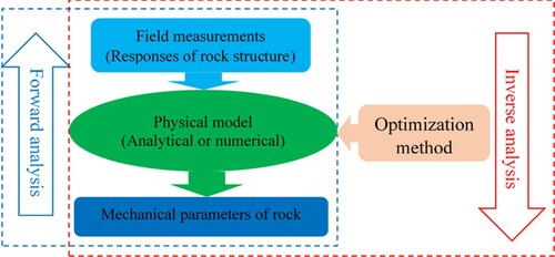
The field measurement data such as displacement, stress, strain, etc., initially are obtained and used to determine the rock mechanical parameters in the inverse analysis. Displacement is easy to obtain in the field and is commonly used in the inverse analysis [5–16]. Zhang and Yin (2014) adopted the pore water pressure in hydraulic fractures to determine the in-situ stress and the elastic modulus of rock mass [17]. Recently, micro-seismic monitoring was paid attention by rock engineering with the development of monitoring technology [18]. Some researchers adopted microseismic data in the inverse analysis to determine the mechanical parameters of rock mass and their damage degree during excavation [19,20]. Inverse analysis has three main components: 1) the field measurements, 2) the physical model (numerical model or analytical model), and 3) the optimization method. Figure 1 shows the forward analysis and inverse analysis. The numerical model plays an important role. However, it is time-consuming, especially for large-scale projects. To improve the efficiency of the inverse analysis, various response surface methods have been built to replace the numerical model for approximating the response of rock structure [5–25]. Soft computing methods such as an artificial neural network (ANN), and support vector machine (SVM) have been successfully applied to approximate the complex relationship between unknown parameters and response of engineering structure [6,9,13–15,17,20–23]. However, both ANN and SVM still have some limitations in their performance [25]. To obtain the acceptable accuracy, the modelling effort or resource demand grows exponentially with the dimensionality of the black-box problems. Therefore, these popular techniques are inappropriate, or even not allowed for modelling high-dimensional problems. To overcome the disadvantage of the above methods, a novel approach of high dimensional model representation (HDMR) was developed in this study to approximate the response of rock mass in the inverse analysis through combining with the response surface method.

Figure 1. The inverse analysis and forward analysis.

HDMR is a general set of quantitative model assessment and analysis tools for capturing the nonlinear, implicit, and high dimensional relationships between sets of input and output variables [26]. HDMR can approximate the high dimensional and nonlinear function using the lower-dimensional function based on optimization and projection operator theory, which can dramatically reduce the sampling effort for learning the input-output behaviour of high dimensional systems. Zhao [27] adopted HDMR to determine the maximum deformation of the implicit limit state function for tunnel reliability analysis [27]. Chowdhury and Rao (2010) applied HDMR to the probabilistic stability assessment of slopes [32]. HDMR has attracted significant attention due to its ability to handle complex high dimensional models. In this study, the HDMR was used to approximate the response of rock mass induced by excavation (displacement, stress, strain, and pressure, etc.). The Excel solver was chosen in the inverse analysis as an optimization tool [17]. The proposed approach was verified and illustrated by two examples of the tunnel. The results indicated that the proposed method improved the efficiency of inverse analysis and provided a good way to deal with the complex response of the tunnel.

In this study, we developed a novel inverse analysis approach to determine the mechanical parameters of rock mass through combing HDMR, numerical model, and response surface. The proposed method met both of the requirements of efficiency and accuracy. The remainder of this study is as follows. First, HDMR and its idea are presented briefly in section 2. The proposed method and its procedure are described in section 3. In section 4, two tunnels are used to verify the proposed method and to illustrate the process of determining the mechanical parameters of the rock mass. The displacement and stress were computed based on the numerical model using the mechanical parameters of rock mass determined by the proposed method. The displacement and stress were in excellent agreement with analytical or numerical solutions. These indicated that the proposed method provided a good way for inverse analysis with both high efficiency and accuracy. Finally, some conclusions are drawn in Section 5.

2. High dimensional model representation (HDMR)

2.1. HDMR

Let the N-dimensional vector x= {x₁, x₂, … x_N} represents the input variables of the model under consideration and also let to show the response variables by g(x). According to the HDMR model [28], the response variables (g(x)) can be expressed as a hierarchical correlated function in terms of the input variables as follows: (1) $\begin{array}{rl}\text{g}(\text{x})& ={\text{g}}_0+\sum _{i=1}^N{g}_i(x_i)+\sum _{1<i_1\le i_2\le N}{g}_{i_1{i}_2}(x_{i_1},x_{i_2})\\ & +\sum _{1<i_1..\le i_l\le N}{g}_{i_1{i}_2\dots i_l}(x_{i_1},x_{i_2},\dots ,x_{i_l})+g_{12\dots N}(x_1,x_2,\dots ,x_N).\end{array}$(1) where g₀ is a constant term representing the 0th order component function of g(x), g_i(x_i) is a 1st order term of g(x) which represents the effect of only variables x_i. $g_{i_1{i}_2}(x_{i_1},x_{i_2})$ is the 2nd order term that represents the cooperative effects of the variables $x_{i_1}$ and $x_{i_2}$. g_12 … N(x₁,x₂, … ,x_N) contains any residual dependence of all the relevant component functions in Equation (1). Once all component functions were determined in Equation (1), the component function constitutes HDMR. Generally, the high order component is negligible. Therefore, HDMR can be employed to approximate the g(x) with high efficiency.

There are two methods to determine the component functions. In this study, cut-HDMR was chosen to determine the component functions in Equation (1) which approximate the implicit limit state function in the inverse analysis. Based on cut-HDMR procedure [28], the first and second-order approximation of g(x), denoted, respectively, by: (2) $\tilde{g}(x)=\sum _{i=1}^{N}g(c_1,\dots ,c_{i-1},x_i,c_{i+1},\dots ,c_N)-(N-1)g(c)$(2)

And (3) $\begin{array}{rl}\tilde{g}(x)& =\sum _{\begin{array}{c}{i}_1=1,i_2=1\\ i_1<i_2\end{array}}^{N}g(c_1,\dots ,c_{i_1-1},x_{i_1},c_{i_1+1},\dots ,c_{i_2-1},x_{i_2},c_{i_2+1},\dots c_N)-(N-2)\\ & \times \sum _{i=1}^{N}g(c_1,\dots ,c_{i-1},x_i,c_{i+1},\dots ,c_N)+\frac{(N-1)(N-2)}{2}g(c).\end{array}$(3) Where c=(c₁,c₂, … ,c_N) is a reference point which is a mean value of the input variables. g(c₁,c₂, … , c_i−1,x_i,c_i+1, … .,c_N) indicates that all the input variables are at their reference point values except x_i. g(c) is the response of system evaluated at the reference point c. $g(c_1,c_2,c_{{\text{i}}_1-1},c_{{\text{i}}_1},c_{{\text{i}}_1+1},\dots c_{{\text{i}}_2-1},c_{{\text{i}}_2},c_{{\text{i}}_2+1},\dots ,c_{\text{N}})$ is evaluated in a plane defined by the binary set of input variables $x_{i_1}$and $x_{i_2}$ through the reference point, etc.

The response of tunnel g(x) at point x can be obtained by the following two steps:

Step 1: Interpolate each of the low-dimensional HDMR terms with respect to the input values of the point x. To the 1st and 2^nd order component function in the HDMR model, n and n² function values were computed based on numerical simulation as follows: (4) $\begin{array}{rl}g(x_i^j)& =g(c_1,\dots ,c_{i-1},x_i^j,c_{i+1},\dots ,c_N),j=1,2,\dots ,n\end{array}$(4) (5) $\begin{array}{rl}g(x_{i_1}^{j_1},x_{i_2}^{j_2})& =g(c_1,\dots ,c_{i_1-1},x_{i_1}^{j_1},c_{i_1+1},\dots ,c_{i_2-1},x_{i_2}^{j_2},c_{i_2+1},\dots c_N),\\ & j_1=1,2,\dots ,n{j}_2=1,2,\dots ,n\end{array}$(5)

Central sample method was applied to construct x_i^j (j=1,2, … ,n) and x_i1j1,x_i2j2. Once n and n² function values were obtained, the 1st and 2^nd component function can be obtained as follows: (6) $\begin{array}{rl}g(x_i)& =\sum _{i=1}^n{\phi }_j(x_i)g(c_1,\dots ,c_{i-1},x_i^j,c_{i+1},\dots ,c_N)\end{array}$(6) (7) $\begin{array}{rl}g(x_{i_1},x_{i_2})& =\sum _{i_1=1}^n\sum _{i_2=1}^n{\phi }_{j_1{j}_2}(x_{i_1},x_{i_2})g(c_1,\dots ,c_{i_1-1},x_{i_1}^{j_1},c_{i_1+1},\dots ,c_{i_2-1},x_{i_2}^{j_2},c_{i_2+1},\dots c_N)\end{array}$(7)

Where φ_j(x_i) and φ_j1j2(x_i1,x_i2) can be obtained using the moving least square method [29]. The same procedure shall be repeated for all the 1st and 2nd component functions, i.e. g_i(x_i) and $g_{i_1{i}_2}(x_{i_1},x_{i_2})$, i,i₁,i₂=1,2, … ,N.

Step 2: Sum the interpolated values of HDMR terms from zeroth order to highest order retained in keeping with the desired accuracy. The response surface of g(x) based on HDMR can be obtained as: (8) $\tilde{g}(x)=\sum _{i=1}^N\sum _{j=1}^n{\phi }_j(x_i)g(c_1,\dots ,c_{i-1},x_i^j,c_{i+1},\dots ,c_N)-(N-1)g_0$(8)

And (9) $\begin{array}{rl}\tilde{g}(x)& =\sum _{\begin{array}{c}{i}_1=1,i_2=1\\ i_1<i_2\end{array}}^N\sum _{i_1=1}^n\sum _{i_2=1}^n{\phi }_{j_1{j}_2}(x_{i_1},x_{i_2})g(c_1,\dots ,c_{i_1-1},x_{i_1}^{j_1},c_{i_1+1},\dots ,c_{i_2-1},x_{i_2}^{j_2},c_{i_2+1},\dots c_N)\\ & -(N-2)\sum _{i=1}^N\sum _{j=1}^n{\phi }_j(x_i)g(c_1,\dots ,c_{i-1},x_i^j,c_{i+1},\dots ,c_N)+\frac{(N-1)(N-2)}{2}{g}_0\end{array}$(9)

2.2. Moving least square method

To determine the coefficient of the component function in Equations (6) and (7), the moving least square method was adopted in this study. Consider a function, u(x) can be approximated using the following form according to moving least square method [29,30]. (10) $u^h(x)=\sum _{i=1}^m{p}_i(x)a_i(x)=p^T(x)a(x)$(10) where $p^T(x)$ is a vector of complete basis function of order m and $a(x)$ is a vector of unknown parameters that depends on x.

The coefficient vector $a(x)$ can be determined by minimizing a weight function, which is defined as: (11) $\text{J}(\text{x})=\sum _{I=1}^{n_t}{w}_I(x)[p^T(x_I)a(x)-d_I{]}^2=[Pa(x)-d{]}^{T}W[Pa(x)-d]$(11) Where x_I stands for the coordinates of sample point I, d with d_I represent the nodal parameter for sample point I, W signifies the weight function associated with sample point I. The stationarity of J(x) with respect to a(x) yields: (12) $\text{A}(\text{x})\text{a}(\text{x})=\text{C}(\text{x})\text{d}$(12) where (13) $\begin{array}{rl}\text{A}(\text{x})& =\sum _{I=1}^{n_t}{w}_I(x)p(x_I)p^T(x_I)=P^{T}WP\end{array}$(13) (14) $\begin{array}{rl}\text{C}(\text{x})& =[w_I(x)p(x_1),\dots ,w_n(x)p(x_n)]=P^{T}W\end{array}$(14)

a(x) can be obtained by solving the above equation and the approximated function u^h(x) will be given by: (15) $u^h(x)=\sum _{I=1}^{n_t}{\phi }_I(x)d_I={\phi }^T(x)d$(15) where (16) $\begin{array}{rl}{\phi }^T(x)& =\{{\phi }_1(x),{\phi }_2(x),\dots ,{\phi }_{n_t}(x)\}=p^T(x)A^{-1}(x)C(x)\end{array}$(16) (17) $\begin{array}{rl}{\phi }_I(x)& =\sum _{j=1}^m{p}_j(x)[A^{-1}(x)C(x){]}_{jI}\end{array}$(17) The above procedure of the moving least square method was implemented in Excel VBA for this study.

3. HDMR based inverse analysis

A numerical model and the optimization method are the two main components of the inverse analysis. In this study, HDMR was applied to replace the numerical model and to approximate the nonlinear function between the response of the tunnel and the mechanical parameters of the rock mass to reduce the computing time significantly. Microsoft solver, implemented in Excel VBA, was considered as an optimization method to search the mechanical parameters of the rock mass.

3.1. HDMR-based response surface

The response surface method (RSM) is a simple mathematical form that approximates the nonlinear implicit function with less computation. To improve the efficiency of inverse analysis, RSM is commonly used to replace the numerical model that is time-consuming. HDMR-based response surface is obtained by combining the RSM and HDMR model. HDMR is adopted to approximate nonlinear implicit function based on RSM. In this study, we used HDMR to approximate the nonlinear relationship between the mechanical parameters of the rock mass (Young's modulus, Poisson's ration, in situ stress) and the response of rock structure (displacement, stress, strain, etc.). The mathematical model of the HDMR-based response surface, HDMR(X), is defined as follows: (18) $\begin{array}{rl}& HDMR(X):R^N\to R^Q,\end{array}$(18) (19) $\begin{array}{rl}& Y=HDMR(X),\end{array}$(19) where X = (x₁, x₂, … , x_N), x_i(i = 1, 2, … , N) is a vector of the mechanical parameters of rock mass and Y = (y₁, y₂, … , y_N) is a Q dimension vector of rock structure response. HDMR(X) can be obtained based on Equation (9) according to the algorithm of HDMR and moving least square method discussed in Section 2.

To obtain HDMR(X), some known sample points are needed. The necessary samples were created for this study by using the numerical model and central samples. Central samples are used to determine 2n + 1 samples in HDMR-based response surface using the following relationship: (20) $x_i={\mu }_i\pm h_i{\sigma }_i$(20) where μ_i is the mean value of the ith unknown parameter, σ_i is the half range of the ith unknown parameter; h_i is a coefficient which is assigned by the user (in general h_i = 1 or 2).

3.2. Optimization method-Excel solver

The optimization method is the key component and influences the efficiency and accuracy of the inverse analysis. Excel solver is a powerful and general-purpose optimization tool. It has a user-friendly interface, and the problem of setting-up is straightforward. Excel also provides a visual development language named Visual Basic for Applications (VBA). It makes it easy to call Excel solver in code and to solve various optimization problems with spreadsheets. Excel solver provides different optimization algorithms such as simplex optimization, gradient optimization, nonlinear programming, evolutionary algorithm, etc. Meanwhile, Excel solver is easy to employ in the inverse analysis to improve practicability [17]. Compared with other optimization methods such as genetic algorithm, particle swarm optimization, etc., it is easier to learn, and also it can reduce a lot of algorithm analysis and code debugging. More importantly, Excel solver has good adaptability and is convenient for solving various optimization problems. In this study, it was adopted to determine the mechanical parameters of rock mass for the inverse analysis.

3.3. Fitness function

The fitness function drives the optimization method to search for the optimal variable. In this study, the difference between the actual and HDMR-based response of rock mass defined the fitness function. The following equation is the definition of the fitness function. (21) $fitness=\sqrt{\sum _{i=1}^n{(y_{pi}-y_i)}^2}$(21) where n is the number of monitored points, y_i is the monitored response of rock mass in the ith key point, and y_pi is the predicted response of rock mass in ith key point.

Computing time depends on the fitness function in the developed method. In the traditional inverse analysis, numerical simulation is the most time-consuming component. In this study, HDMR was adopted to replace numerical simulation. The total inverse analysis time depends on the computing time of the sample point. The computing time of the sample points depends on the scale of the problem. Once established the HDMR model, the computing time of fitness is of no account and has nothing to do with the computing time of the sample point.

3.4. Procedure for HDMR-based inverse analysis

In this study, HDMR was used to approximate the nonlinear relationship between the mechanical parameters of rock mass and the response of rock structure through combining with the response surface method and numerical model. Excel solver was adopted to search the mechanical parameters of the rock mass. HDMR-based inverse analysis improves efficiency with high accuracy. The following explained the procedure of the proposed inverse analysis (Figure 2).

Figure 2. The flowchart of the developed approach.

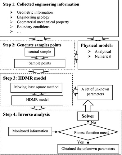
Step 1: Determine the engineering information and data such as the unknowns (need to be determined by inverse analysis), known parameters, numerical model and its boundary conditions, the component function of HDMR, and the range of parameters to be determined.

Step 2: Generate the sample points using the central sample method, and calculate the response of rock structure at each sample point. Sample sets consist of the sample points and their response.

Step 3: Based on the above samples, determine the HDMR-based response surface to approximate the nonlinear function between the mechanical parameters of rock mass and the corresponding response of rock structure. Moving least square method was employed to determine the coefficient of component function in the HDMR model.

Step 4: Build the fitness function and activate the Excel solver to search the mechanical parameters of rock mass based on the monitored response in rock engineering.

4. Numerical examples

4.1. A circular tunnel under hydrostatic stress field

Suppose that a circular tunnel is excavated in a continuous, homogeneous, isotropic, initially elastic rock mass subjected to hydrostatic far-field stress p₀ and uniform support pressure p_i as shown in Figure 3. While p_i is less than the critical pressure p_cr, a plastic zone exists. The values of p_cr are obtained from the following equations: (22) ${\text{p}}_{\text{cr}}=\frac{2{\text{p}}_0-{\sigma }_{\text{c}}}{\text{k}+1}$(22) where ${\sigma }_{\text{c}}$ is the uniaxial compression strength which can be determined by the following equation: (23) ${\sigma }_{\text{c}}=\frac{\text{c}(\text{k}-1)}{\tan \phi }$(23) Where φ is the internal friction angle, and c is the cohesion and $\text{k}=\frac{1+\sin \phi }{1-\sin \phi }$.

Figure 3. A circular tunnel subjected to hydrostatic far-field stress.

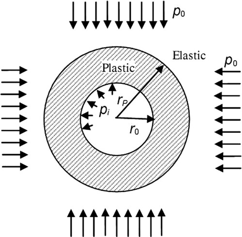
Duncan (1993) obtained the plastic zone radius r_p and the inward displacement of tunnel wall u_ip based on the Mohr-Coulomb criterion [31]. (24) $\begin{array}{rl}\frac{{\text{r}}_{\text{p}}}{{\text{r}}_0}& ={\left[\frac{2({\text{p}}_0+\text{s})}{(\text{k}+1)({\text{p}}_{\text{i}}+\text{s})}\right]}^{1/(\text{k}-1)},\end{array}$(24) (25) $\begin{array}{rl}\frac{{\text{u}}_{\text{ip}}}{{\text{r}}_0}& =\left[\frac{1+\mu }{\text{E}}\right]\left[2(1-\mu )({\text{p}}_0-{\text{p}}_{\text{cr})}{\left(\frac{{\text{r}}_{\text{p}}}{{\text{r}}_0}\right)}^2-2(1-2\mu )({\text{p}}_0-{\text{p}}_{\text{i}})\right],\end{array}$(25) where E is the elastic modulus and μ is Poisson's ratio. The values of s are obtained from the following equations: (26) $\text{s}=\frac{{\sigma }_{\text{c}}}{\text{k}-1},$(26)

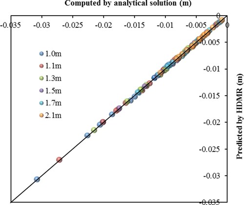
In this study, far-field stress p_0, cohesion c, and internal friction angle φ needed to be determined using inverse analysis. Displacement of the tunnel is the response of the rock structure. Six monitored points, where was in the horizontal direction, were used in a circular tunnel. The distance between the centre of the tunnel and the monitored points was 1.0, 1.1, 1.3, 1.5, 1.7, and 2.1 m, respectively. The above formula (Equation 25) was adopted to compute the displacements of the monitored points in the tunnel. The radius of the tunnel was 1.0 m. The value of far-field stress p_0, elastic modulus E, cohesion c, and internal friction angle φ were 30 MPa, 7 GPa, 3.45 MPa, and 30^o, respectively. The displacements of six monitored points were computed and used as field measurements to determine the unknown mechanical parameters of rock mass using the proposed method. Based on the proposed method, the sample points were built and presented in Table 1.

Table 1. Sample points.

		Numerical integration grid				Outputs (displacement of monitored site (m))
						Distance to the centre of tunnel(m)
Variables	No.	p0/MPa	E/MPa	c /MPa	φ/^o	1.00	1.10	1.30	1.50	1.70	2.1
p0/MPa	1	10	7000	3.45	30	−0.0019	−0.0017	−0.0014	−0.0012	−0.0011	−0.0009
	2	20	7000	3.45	30	−0.0057	−0.0049	−0.0039	−0.0033	−0.0029	−0.0023
	3	30	7000	3.45	30	−0.0118	−0.0103	−0.0080	−0.0065	−0.0055	−0.0045
	4	40	7000	3.45	30	−0.0201	−0.0177	−0.0139	−0.0112	−0.0093	−0.0073
	5	50	7000	3.45	30	−0.0308	−0.0272	−0.0216	−0.0175	−0.0145	−0.0108
E/MPa	1	30	4000	3.45	30	−0.0206	−0.0180	−0.0140	−0.0113	−0.0096	−0.0078
	2	30	5500	3.45	30	−0.0150	−0.0131	−0.0102	−0.0082	−0.0070	−0.0057
	3	30	7000	3.45	30	−0.0118	−0.0103	−0.0080	−0.0065	−0.0055	−0.0045
	4	30	8500	3.45	30	−0.0097	−0.0085	−0.0066	−0.0053	−0.0045	−0.0037
	5	30	10000	3.45	30	−0.0082	−0.0072	−0.0056	−0.0045	−0.0039	−0.0031
c /MPa	1	30	7000	2.05	30	−0.0186	−0.0165	−0.0131	−0.0106	−0.0088	−0.0065
	2	30	7000	2.75	30	−0.0143	−0.0126	−0.0098	−0.0079	−0.0066	−0.0052
	3	30	7000	3.45	30	−0.0118	−0.0103	−0.0080	−0.0065	−0.0055	−0.0045
	4	30	7000	4.15	30	−0.0101	−0.0088	−0.0068	−0.0056	−0.0049	−0.0040
	5	30	7000	4.85	30	−0.0090	−0.0078	−0.0061	−0.0051	−0.0045	−0.0036
φ/^o	1	30	7000	3.45	20	−0.0226	−0.0201	−0.0162	−0.0133	−0.0112	−0.0082
	2	30	7000	3.45	25	−0.0156	−0.0138	−0.0109	−0.0088	−0.0073	−0.0056
	3	30	7000	3.45	30	−0.0118	−0.0103	−0.0080	−0.0065	−0.0055	−0.0045
	4	30	7000	3.45	35	−0.0094	−0.0082	−0.0063	−0.0053	−0.0046	−0.0038
	5	30	7000	3.45	40	−0.0079	−0.0068	−0.0054	−0.0046	−0.0041	−0.0033

HDMR-based response surface was built based on the above sample points. Figure 4 shows the displacement comparison between those predicted by HDMR and those computed by analytical solution (Equation 25). The computed displacement using HDMR was in excellent agreement with the analytical solution. It demonstrated that the HDMR-based response surface presented the nonlinear relationship between unknown parameters and the displacement of the tunnel well. Thus, it was feasible to replace the analytical solution using the HDMR-based response surface method.

Figure 4. Displacement comparison between HDMR model and the analytical solution.

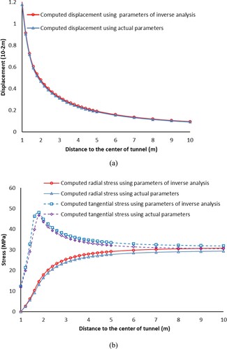
The HDMR-based inverse analysis was used to determine the unknown parameters using the above HDMR model and the computed displacement. The determined value of far-field stress p₀, elastic modulus E, cohesion c, and internal friction angle φ were 30 MPa, 7 GPa, 3.45 MPa, and 30^o, respectively. The relative error was 4.62%, 3.21%, 0.64%, and 6.90%, respectively. The maximum relative error was less than 7%. It indicated that the predicted parameters agreed well with the real parameters using the proposed method. The comparison between the displacements obtained based on predicted, HDMR, and real parameters are presented in Figure 5. Figure 6 exhibits the stress and displacement comparison of the surrounding rock mass of the tunnel based on predicted and real parameters. The results revealed that the proposed approach can be used to determine the mechanical parameters of the rock mass for rock mechanics and engineering.

Figure 5. Displacement comparison at monitored point using different methods.

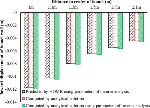
Figure 6. Displacement and stress comparison of surrounding rock mass of tunnel. (a) Displacement. (b) Stress.

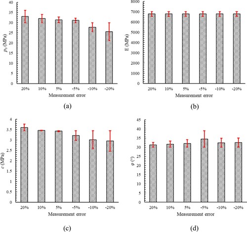
The measurement error is inevitable in rock engineering. The robust algorithm is critical to the inverse analysis. In this study, we assumed the error in displacement measurement was −20%, −10%, −5%, 5%, 10%, 20%, respectively. Figure 7 shows the relationship between the measurement error and the obtained mechanical parameters. We can see that the measurement error had some influences on the far-field stress, cohesion, and internal friction angle. The relative error between estimated by the inverse analysis and the real value increased with the increase in measurement error. However, the maximum relative error was less than 15% when the measurement error was 20%. The measurement error had little impact on the elastic modulus. The maximum relative error was less than 4%. Therefore, the developed method has certain strong advantages. However, it is very critical to enhance the accuracy of monitored technology.

Figure 7 The effect of the measurement error on results. (a) Far-field stress (p₀). (b) Elastic Young's modulus (E). Cohesion (c). (d) Internal friction angle (φ).

4.2. A horseshoe tunnel

In this example, a horseshoe tunnel without an analytical solution was applied to illustrate the performance of the proposed method. The span and height of the tunnel were about 5 m (Figure 8). A numerical model was adopted to build the HDMR-response surface. In this study, Phase 2 software was adopted to compute the displacement of the tunnel. The model size was 31 m × 31 m. The rock was assumed to be linearly elastic and perfectly plastic. The Mohr-Column yield criterion was employed. Plane strain conditions were also assumed. The boundary conditions were defined such that the normal direction of the outer boundary was fixed. The model was discretized into 1,485 elements and 822 nodes. The computing time of a sample point was about 5 s. In this study, the developed method was adopted to determine the initial geo-stress and Young's modulus. The cohesion, internal friction angle, and Poisson's ratio of rock were 1, 31.45 MPa, and 0.3, respectively. Table 2 present the sample points for the HDMR model. Figure 9 indicates the displacement comparison between those predicted by HDMR and those computed by the numerical model. The predicted displacements using the HDMR were very close to those of the numerical solution. It proved that the HDMR-based response surface presented well the nonlinear relationship between unknown parameters and displacement of the tunnel. Hence, it can be used to replace the numerical model.

Figure 8. The mesh of the horseshoe tunnel.

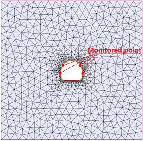
Figure 9. Displacement comparison between HDMR model and numerical model.

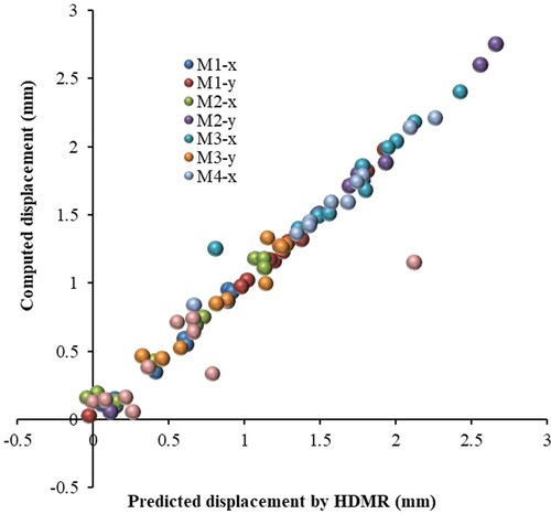
Table 2. Sample points for horseshoe tunnel.

		Numerical integration grid			Outputs (Displacement of monitored site)
					1		2		3		4
Variable	No.	E(GPa)	σx(MPa)	σy(MPa)	x	y	x	y	x	y	x	y
E(GPa)	1	12	12	8	0.8920	1.9600	1.1300	2.8500	2.8000	1.5000	2.6000	0.3720
	2	16	12	8	0.6660	1.4600	0.8430	2.1300	2.1300	1.1200	1.9100	0.2890
	3	20	12	8	0.5440	1.1700	0.6790	1.7100	1.7000	0.8850	1.5600	0.2250
	4	24	12	8	0.4410	0.9780	0.5650	1.4200	1.3900	0.7040	1.3000	0.2490
	5	28	12	8	0.3850	0.8370	0.4840	1.2100	1.2000	0.6020	1.1100	0.2100
σx(MPa)	1	20	8	8	0.0051	1.0800	0.0054	1.5000	1.1400	0.2940	1.1400	0.2360
	2	20	10	8	0.2720	1.1200	0.0341	1.5000	1.4200	0.5880	1.3500	0.0304
	3	20	12	8	0.5440	1.1700	0.6790	1.7100	1.7000	0.8850	1.5600	0.2250
	4	20	14	8	0.7990	1.2200	1.0100	1.8100	1.9400	1.1900	1.7600	0.5420
	5	20	16	8	1.0800	1.2600	1.3600	1.9100	2.2100	1.5000	1.9600	0.8280
σy(MPa)	1	20	12	4	1.0600	0.7150	1.3500	1.1700	1.6100	1.3100	1.3900	0.9350
	2	20	12	6	0.8020	0.9420	1.0100	1.4400	1.6400	1.0700	1.4700	0.6110
	3	20	12	8	0.5440	1.1700	0.6790	1.7100	1.7000	0.8850	1.5600	0.2250
	4	20	12	10	0.2750	1.4100	0.3390	1.9800	1.7200	0.6070	1.6300	0.0330
	5	20	12	12	0.0137	1.6300	0.0073	2.2500	1.7200	0.3610	1.7200	0.3530

To verify the HDMR-based inverse analysis, suppose there are two cases with different initial geo-stress and Young's modulus as presented in. Displacement values in the key points, calculated by the numerical method, were regarded as the measurement displacement. The initial geo-stress and Young's modulus were determined using HDMR-based inverse analysis based on the displacements shown in. Figure 10 shows the comparisons between the actual value and the determined value by inverse analysis. The maximum relative error was less than 8%. It indicated that the determined parameters by inverse analysis agreed well with the actual parameters using HDMR-based inverse analysis. The time of inverse analysis was about 10 s for the horseshoe tunnel Table 3.

Figure 10. The comparison between actual parameters and determined parameters by inverse analysis. (a) Case 1. (b) Case 2.

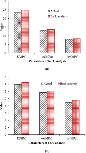
Table 3. The unknown parameters and corresponding displacement in two cases.

				Displacement (cm)
				1		2		3		4
	E (GPa)	σx(MPa)	σy(MPa)	x	y	x	y	x	y	x	y
Case 1	23.35	13.16	7.98	0.59	1.02	0.75	1.50	1.51	0.88	1.42	0.38
Case 2	13.90	11.70	8.88	0.55	1.82	0.69	2.60	2.40	1.00	2.21	0.16

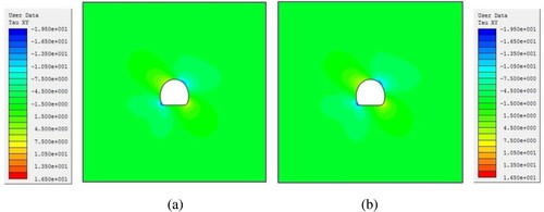
Figure 11 presents the displacements comparison using a different method at the monitored point. It shows that the computed displacement based on the determined parameters by inverse analysis was in excellent agreement with the measured displacement. Figure 12 displays the deformation contour of the surrounding rock mass for the tunnel. Figures 13–15 show the stress contour of the surrounding rock mass of the tunnel based on determined parameters by inverse analysis and real parameters. The obtained mechanical parameters of rock mass characterized mechanical behaviour well (Figures 13 and 14). The estimated stress was in excellent agreement with the real value in the wall of the tunnel. Although there was a little difference in the horizontal and vertical stresses as it moved away from the tunnel wall to determine the mechanical parameters of rock based on the displacement of the tunnel wall. The results demonstrated that the proposed approach determines the mechanical parameters of rock mass for real rock engineering.

Figure 11. Displacement comparison using different methods. (a) Case1. (b) Case2.

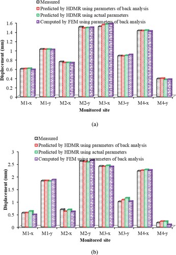
Figure 12. The deformation contour of surrounding rock mass based on actual parameters and determined parameters by inverse analysis for tunnel. (a) Actual parameters. (b) Inverse analysis.

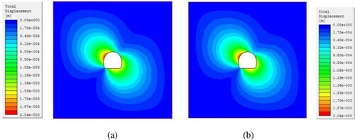
Figure 13. The horizontal stress contour of surrounding rock mass based on actual parameters and determined parameters by inverse analysis for tunnel. (a) Actual parameters. (b) Inverse analysis.

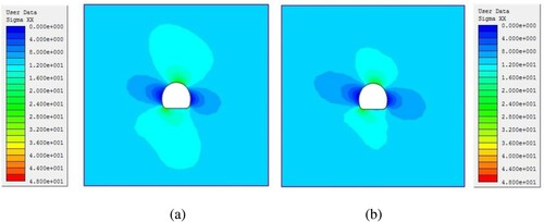
Figure 14. The vertical stress contour of surrounding rock mass based on actual parameters and determined parameters by inverse analysis for tunnel. (a) Actual parameters. (b) Inverse analysis.

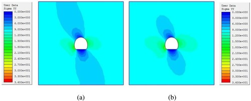
Figure 15. The shear stress contour of surrounding rock mass based on actual parameters and determined parameters by inverse analysis for tunnel. (a) Actual parameters. (b) Inverse analysis.

5. Conclusion

In this study, a novel inverse analysis method was proposed. The methods combined HDMR and numerical model. HDMR was adopted to present the nonlinear relationship between the mechanical parameters of rock mass and the displacement of the tunnel. Also, it determined the in situ stress and mechanical parameters of rock mass for the two tunnel examples successfully. The determined parameters by the inverse analysis were compared with the real parameters. The deformation of surrounding rock mass and stress distribution were also compared. The results indicated that the proposed method was practical and accurate. Moreover, the proposed method made it convenient to be applied to determine the in situ stress and mechanical parameters of rock mass from the monitored data. The major conclusions of this study are summarized as follows:

(1) There was less parameter to determine in the HDMR algorithm. Meanwhile, HDMR could present well the nonlinear relationship between mechanical parameters of rock mass and the response of rock structure. Thus, HDMR could replace the numerical method in inverse analysis. It was critical to the practical rock engineering in which it was difficult to obtain the analytical solution of rock structure response.

(2) The inverse analysis is a reliable tool that is commonly used in rock engineering. However, it is time-consuming for large-scale projects and hinders the application in practical rock engineering. HDMR reduced the computing time with high accuracy and enhanced the efficiency of inverse analysis.

(3) Excel solver was an excellent and user-friendly optimization tool. Excel solver was adopted in HDMR-based inverse analysis as an optimization method to determine the mechanical parameters of the rock mass. It provided an excellent and promising tool for inverse analysis for practical rock engineering.

Disclosure statement

No potential conflict of interest was reported by the author(s).

References

- Jing L, Hudson JA. Numerical methods in rock mechanics. Int J Rock Mech Min Sci. 2002;39(4):409–427.
- Wei MD, Dai F, Xu NW, et al. Experimental and numerical study on the fracture process zone and fracture toughness determination for ISRM-suggested semi-circular bend rock specimen. Eng Fract Mech. 2016;154:43–56.
- Wei MD, Dai F, Xu NW, et al. An experimental and theoretical assessment of semi-circular bend specimens with chevron and straight-through notches for mode I fracture toughness testing of rocks. Int J Rock Mech Min Sci. 2017;99:28–38.
- Sakurai S. Back analysis in rock engineering. Leiden: CRC press; 2017.
- Feng ZL, Lewis RW. Optimal estimation of in-situ ground stress from displacement measurements. Int J Numer Anal Method Geomech. 1987;11(4):397–408.
- Feng XT, Zhao HB, Li SJ. A new displacement back analysis to identify mechanical geo–material parameters based on hybrid intelligent methodology. Int J Numer Anal Method Geomech. 2004;28(11):1141–1165.
- Mccarron WO. Plasticity model for cyclic axial pile response with back-analyses of West Delta pile tests. Int J Geomech. 2017;17(4):04016099.
- Oreste P. Back analysis techniques for the improvement of the understanding of rock in underground constructions. Tunnel Underground Space Technol. 2005;20(1):7–21.
- Pichler B, Lackner R, Mang HA. Back analysis of model parameters in geotechnical engineering by means of soft computing. Int J Numer Meth Eng. 2003;57(14):1943–1978.
- Sakurai S, Takeuchi K. Back analysis of measured displacements of tunnels. Rock Mech Rock Eng. 1983;16:173–180.
- Vardakos S, Gutierrez M, Xia CC. Parameter identification in numerical modeling of tunneling using the Differential Evolution genetic algorithm DEGA. Tunnel Underground Space Technol. 2012;28:109–123.
- Yazdi JS, Kalantary F, Yazdi HS. Calibration of soil model parameters using particle swarm optimization. Int J Geomech. 2012;12(3):229–238.
- Yu YZ, Zhang BY, Yuan HN. An intelligent displacement back–analysis method for earth–rockfill dams. Comput Geotech. 2007;34(6):423–434.
- Zhang S, Yin S. Determination of in situ stresses and elastic parameters from hydraulic fracturing tests by geomechanics modeling and soft computing. J Pet Sci Eng. 2014;124:484–492.
- Zhao H, Yin S. Inverse analysis of geomechanical parameters by artificial bee colony algorithm and multi-output support vector machine. Inverse Probl Sci Eng. 2016;24(7):1266–1281.
- Zhao HB, Yin SD. Geomechanical parameters identification by particle swarm optimization and support vector machine. Appl Math Modell. 2009;33(10):3997–4012.
- Zhao H, Ru Z, Yin S. A practical indirect back analysis approach for geomechanical parameters identification. Mar Georesour Geotechnol. 2015;33(3):212–221.
- Li A, Liu Y, Dai F, et al. Continuum analysis of the structurally controlled displacements for large-scale underground caverns in bedded rock masses. Tunnell Underground Space Technol. 2020;97:103288.
- Zhao Y, Tang T, Yu Q, et al. Dynamic reduction of rock mass mechanical parameters based on numerical simulation and microseismic data–A case study. Tunnell Underground Space Technol. 2019;83:437–451.
- Zhang Y, Su G, Li Y, et al. Displacement back-analysis of rock mass parameters for underground caverns using a novel intelligent optimization method. Int J Geomech. 2020;20(5):04020035.
- Rahul Y, Swapnil T, Shailendra A, et al. A combined neural network and simulated annealing based inverse technique to optimize the heat source control parameters in heat treatment furnaces. Inverse Probl Sci Eng. 2020;28(9):1265–1286.
- Jader LJ, Antônio JSN, César CS. A hybrid approach with artificial neural networks, Levenberg–marquardt and simulated annealing methods for the solution of gas–liquid adsorption inverse problems. Inverse Probl Sci Eng. 2009;17(1):85–96.
- Ebrahim K, Naser K, Esmaeel K. Identification of linear and non-linear physical parameters of multistory shear buildings using artificial neural network. Inverse Probl Sci Eng. 2015;23(4):670–687.
- Deng JH, Lee CF. Displacement back analysis for a steep slope at the three Gorges Project site. Int J Rock Mech Min Sci. 2001;38(2):259–268.
- Zhao H, Yin S, Ru Z. Relevance vector machine applied to slope stability analysis. Int J Numer Anal Meth Geomech. 2012;36(5):643–652.
- Rabitz H, Alis OF. General foundations of high dimensional model representations. J Math Chem. 1999;25(2-3):197–233.
- Zhao H. High dimension model representation-based response surface for reliability analysis of tunnel. Mech Probl Eng. 2018;2018:8049139.
- Ramberg J, Schmeiser B. An approximate method for generating asymmetric random variables. Commun Assoc Comput Mach. 1974;17(2):78–82.
- Li G, Wang SW, Rabitz H. High dimensional model representations generated from low dimensional data samples-I. mp-cut-HDMR. J Math Chem. 2001;30(1):1–30.
- Lancaster P, Salkauskas K. Curve and surface fitting: An Introduction. London: Academic Press; 1986.
- Duncan FME. Numerical modeling of yield zones in weak rocks. In: Hudson JA, editor. Comprehensive rock engineering, vol. 2. Oxford: Pergamon; 1993. p. 49–75.
- Chowdhury R, Rao BN. Probabilistic stability assessment of slopes using high dimensional model representation. Comput Geotech. 2010; 37(7-8):876-884.