Approximation error model (AEM) approach with hybrid methods in the forward-inverse analysis of the transesterification reaction in 3D-microreactors

Abstract

This work advances the approximation error model approach for the inverse analysis of the biodiesel synthesis using soybean oil and methanol in 3D-microreactors. Two hybrid numerical-analytical approaches of reduced computational cost are considered to offer an approximate forward problem solution for a three-dimensional nonlinear coupled diffusive-convective-reactive model. First, the Generalized Integral Transform Technique (GITT) is applied using approximate non-converged solutions of the 3D model, by adopting low truncation orders in the eigenfunction expansions. Second, the Coupled Integral Equations Approach (CIEA) provides a reduced mathematical model for the average concentrations, which leads to inherently approximate solutions. The AEM approach through the Bayesian framework is illustrated in the simultaneous estimation of kinetic and diffusion coefficients of the transesterification reaction. For this purpose, the fully converged GITT results with higher truncation orders for the 3D partial differential model are employed as reference results to define the approximations errors. The results highlight that either the non-converged solutions via GITT or the reduced model solution obtained via CIEA, when taking into account the model error, are robust and cost-effective alternatives for the inverse analysis of nonlinear convection–diffusion-reaction problems.

KEYWORDS:

• Approximation error model
• integral transforms
• improved lumped approach
• GITT
• CIEA
• MCMC
• hybrid methods
• microreactors
• biodiesel synthesis

Nomenclature

${\text{C}}^{\ast }$	=	dimensional concentration, mol m−3
$\text{C}$	=	dimensionless concentration
${\text{D}}^{\ast }$	=	diffusion coefficient, m2 s−1
D	=	diffusion parameter in the exponential format
$\mathbf{e}$	=	vectors containing the measure error derived randomly from a known distribution function
$\overline{\mathbf{e}}$	=	vectors containing the mean values of the measurement error distribution
$\text{G}$	=	kinetic terms
$\text{H}$	=	total height of the microreactor, m
${\text{H}}_{\text{TG}}$	=	interface position inside the microreactor, m
$\mathbf{J}$	=	sensitivity matrix
$\text{j}$	=	reduced sensitivity coefficient
$\text{k}$	=	kinetic constants, m3 mol−1 s−1
$\text{L}$	=	total length of the microreactor, m
$\text{N}$	=	number of measurements
$\text{n}$	=	number of parameters to be estimated
$\text{NT}$	=	truncation order of the transformed system
$\text{nt}$	=	number of accepted states in the MCMC method
$\mathbf{p}$	=	vector of parameters
$\overline{\mathbf{p}}$	=	vectors containing the mean values of $\mathbf{p}$
${\mathbf{p}}^{\ast }$	=	candidate vector of parameter in the MCMC method
$\text{q}$	=	probability distribution function
$\text{Q}$	=	volumetric flow rate, m3 s−1
$\text{U}$	=	dimensionless velocity profile or uniform distribution
$\text{u}$	=	dimensional velocity profile, m s−1
Vol	=	volume, m3
$\text{W}$	=	total width of the microreactor, m
$\mathbf{W}$	=	covariance matrix for experimental measurements error
${\mathbf{W}}_{\text{Ap}}$	=	covariance matrix for approximation error
${\mathbf{W}}_{\text{p}}$	=	covariance matrix for parameters
$\tilde{\mathbf{W}}$	=	covariance matrix combining the experimental and approximation errors
$\text{x, y, z}$	=	dimensional spatial coordinate, m
$\text{X, Y, Z}$	=	dimensionless spatial coordinate
$\mathbf{y}$	=	vector of measurements

Greek symbols

$\alpha$	=	search step in the MCMC method
$\mu$	=	dynamic viscosity, Pa. s
$\xi$,$\varsigma$,$\omega$	=	dimensionless group
$\rho$	=	density, kg m-3
$\mathit{\epsilon }$	=	vector containing the model approximation error
$\epsilon$	=	increment for calculus of derivative
$\kappa$	=	kinetic parameter in the exponential format
$\mathit{\eta }$	=	distribution of measurements and approximate errors
$\overline{\mathit{\eta }}$	=	vector with the mean values of $\mathit{\eta }$
$\mathbf{\Gamma }$	=	covariance matrix of $\mathbf{p}$
${\mathbf{\Gamma }}_{\eta \mathbf{p}}$	=	covariance matrix of $\mathit{\eta }$ and $\mathbf{p}$
$\sigma$	=	standard deviation
$\hat{\sigma }$	=	reference standard deviation
$\tau$	=	residence time, min
$\pi$	=	probability distribution function

Subscripts and superscripts

$\text{A}$	=	referring to the alcohol
$\text{Ac}$	=	referring to the accurate solution
Av	=	referring to the average potential
$\text{Ap}$	=	referring to the approximate solution
$\text{B}$	=	referring to the biodiesel
$\text{DG}$	=	referring to the diglyceride
$\text{Exp}$	=	referring to the experimental measurements
$\text{GL}$	=	referring to the glycerol
$\text{i}$	=	counter
$\text{MG}$	=	referring to the monoglyceride
$\text{p}$	=	referring to intermediates and products of reaction
$\text{s}$	=	referring to the species
$\text{Sim}$	=	referring to the simulated measurements
$\text{TG}$	=	referring to the triglyceride

1. Introduction

Inverse analysis has great relevance in engineering and physical sciences, with its mathematical and statistical background being readily available in various sources [1–7]. The MCMC method is a widely used Bayesian method that allows the statistical inference about unknown parameters from its posterior probability density, considering the measurements and the related uncertainties through the likelihood function and any prior information from the unknown parameters [3,4,6,8]. This method is especially suitable when it is unfeasible to find an analytical solvable posterior distribution and/or a large parameter space is involved, allowing for the Bayesian inference application even in rich and complex models. To speed up the MCMC calculations, approximate solutions can replace a more accurate forward problem treatment meeting constraints in the computing time, but at the same time ensuring accuracy in the inverse analysis, by using the so-called Approximation Error Model (AEM) approach. The error when approximate forward solutions are used can be accounted through statistical quantities obtained from a sampling procedure of the difference between approximate and accurate solutions. Such information can then be inserted in the likelihood function as an approximation error [5,9–17].

In this work, a robust and efficient statistical inversion approach is implemented to estimate the kinetic and diffusion coefficients of the biodiesel synthesis in 3D-microreactors within the Bayesian framework through the Metropolis-Hastings algorithm in the Markov Chain Monte Carlo (MCMC) method. Forward analysis for diffusive-convective-reactive processes governed by nonlinear coupled multidimensional mathematical models is not a straightforward computational task and hybrid techniques are particularly attractive since they combine numerical and analytical approaches to construct more accurate and cost-effective solutions, as compared to purely numerical approaches. The so-called Generalized Integral Transform Technique (GITT) is an example of a hybrid method that has been successfully applied in the solution of various flow, heat and mass transfer problems [18–32]. Derived from the Classical Integral Transform Technique (CITT) [33,34], the GITT is based on analytical eigenfunction expansions and numerical transformed potentials, obtained, respectively, from the solution of a suitable eigenvalue problem and of an infinite nonlinear coupled ordinary differential system. This transformed system usually depends on a single independent variable, and, therefore, its numerical solution demands much less computational effort than the original multi-dimensional model, making the GITT a successful technique for performing the time-consuming computational task inherent to inverse analysis [27,35–43].

Another interesting alternative of reducing the computational effort in forward-inverse analysis is the so-called Coupled Integral Equations Approach – CIEA [23,44–49,64]. The CIEA is a problem reformulation tool that has been employed in the simplification of diffusion and convection–diffusion problems via averaging processes in one or more of the involved space coordinates. The resulting lumped-differential formulations offer substantial improvement over classical lumping schemes in terms of accuracy, without introducing additional mathematical complexity in the corresponding final simplified differential equations to be handled. The CIEA has also been successfully applied to a few forward-inverse analyses in different contexts [13,14,49,64], where it should be pointed out the contribution in combining the improved lumped-differential formulation with the Approximation Error Model [14,15].

The idea of combining the AEM with hybrid methods is here further explored. The physical problem used to demonstrate the proposed combined approach is the biodiesel synthesis in microreactors via the transesterification reaction, which is a process that has been widely explored in the literature due to the high conversion rate of triglyceride obtained with low residence time and temperature levels compared to traditional processes performed in conventional batch reactors [49–55,63,64]. Biodiesel is generally defined as the mono alkyl esters of long chain fatty acids derived mainly from the transesterification reaction between triglycerides, obtained from renewable raw materials such as vegetable oils or animal fats, and alcohol, usually methanol or ethanol, in the presence of a catalyst [53,56]. It is considered a non-toxic and biodegradable product with physical–chemical properties very similar to those of conventional diesel and that presents low emissions of carbon, sulfur, particulate matter and unburned hydrocarbons [53,57,58]. Microreactors favour the reaction of the immiscible reagents in the transesterification, since the molecular diffusive effects occur more rapidly due to the significant reduction in the diffusion path length [59], resulting in more effective mass and heat transfer processes. However, due to the complexity of this application, many effects influence the biodiesel yields, such as the complex liquid–liquid interaction established in the reactive system, the reaction kinetic mechanism, the solubility of the components [60], the types of reagents and their molar feed ratio, the temperature of the system and the types and concentration of the catalysts, posing some difficulties to develop an optimized design of the microreactors for the biodiesel production. Thus, computational simulation plays a crucial role in determining the chemical kinetic and diffusion coefficients and, for that purpose, mathematical models and methodologies for forward-inverse analysis have been addressed in the literature [49,50,55,58,61–64].

The goal of this work is to simultaneously estimate the kinetic and diffusion coefficients of the transesterification with soybean oil and methanol in microreactors, by using simulated experimental data and approximate solutions obtained from a diffusive-convective-reactive nonlinear multicomponent 3D model [49,55]. The fully converged solutions derived through the GITT approach from the 3D mathematical model are considered as the accurate reference results [55]. Two alternative low-cost approximate solutions are then explored, one from a reduced model derived by the CIEA and the other directly obtained from the GITT approach, but considering non-converged solution with low truncation orders in the eigenfunction expansions. The error analysis is performed only once, within a prior range considered for the parameters, and then approximate solutions combined with the approximation error approach are used in the inverse analysis leading to a significant reduction in the overall computational time. A sensitivity analysis together with the sequential experimental design are also presented to identify possible linear dependence among the parameters and to identify which residence times should be chosen to take the experimental measurements. In light of experimental limitations, only data on the average concentrations of four species at the microreactor outlet are considered to be available, for a few values of residence time, from the simulated data.

2. Forward-Problem: formulation and solution methodology

The forward-problem here addressed has been posed in [55] and it consists in determining the concentration profile of the species involved in the transesterification in microreactors from the knowledge of inlet and boundary conditions, reaction mechanism, geometry and parameters of the physico-chemical process.

The mathematical model for the biodiesel production in microreactors considers the hypothesis of continuous fully developed stratified laminar and incompressible flow of oil and alcohol, both as Newtonian fluids, where the significant reactive effects occur only in the oil phase [50,55]. Figure 1 illustrates a scheme of the velocity profile for the stratified flow of oil and alcohol in a microsystem obtained from the analytical solution based on the Classical Integral Transform Technique (CITT) [55].

Figure 1. Scheme of the velocity profile for the fully developed stratified flow between oil (soybean) and alcohol (methanol) within a microreactor.

Since this mathematical model assumes that the reaction is carried out mainly in the oil phase, the residence time $\tau$ can be written as a ratio between the volume and the volumetric flow rate of the oil species, in the form: (1) $\begin{array}{rl}& \tau =\frac{\text{Vo}{\text{l}}_{\text{TG}}}{{\text{Q}}_{\text{TG}}}=\frac{\text{LW}{\text{H}}_{\text{TG}}}{{\text{Q}}_{\text{TG}}}\end{array}$(1) where $\text{Vo}{\text{l}}_{\text{TG}}$ is the volume of oil layer, ${\text{Q}}_{\text{TG}}$ is the oil volumetric flow rate, $\text{L}$ and $\text{W}$ are the length and width of the microreactor, and ${\text{H}}_{\text{TG}}$ is the position of the interface between the oil and the alcohol. Different volumetric flow rates lead to different residence times. By assuming the transesterification as a second order and reversible reaction [50,55,56], the dimensionless mathematical model for the concentration of the species in the transesterification mass transfer problem is then given by [55]: (2a) $\begin{array}{rl}& {\text{U}}_{\text{TG}}(\text{Y,Z})\frac{\mathrm{\partial }{\text{C}}_{\text{s}}(\text{X,Y,Z})}{\mathrm{\partial }\text{X}}={\xi }_{\text{s}}\left(\frac{{\mathrm{\partial }}^2{\text{C}}_{\text{s}}}{\mathrm{\partial }{\text{Y}}^{\text{2}}}+\omega \frac{{\mathrm{\partial }}^2{\text{C}}_{\text{s}}}{\mathrm{\partial }{\text{Z}}^{\text{2}}}\right)+\varsigma {\text{G}}_{\text{s}},\text{where s}=\text{TG,DG,MG,B,A,GL}\end{array}$(2a) (2b,c) $\begin{array}{rl}& {\text{C}}_{\text{TG}}(\text{0,Y,Z})=1,{\text{C}}_{\text{s}}(\text{0,Y,Z})=0,\text{where s}=\text{DG,MG,B,A,GL}\end{array}$(2b,c) (2d-f) $\begin{array}{rl}& {\frac{\mathrm{\partial }{\text{C}}_{\text{s}}}{\mathrm{\partial }\text{Y}}|}_{\text{Y}=0}={\frac{\mathrm{\partial }{\text{C}}_{\text{s}}}{\mathrm{\partial }\text{Z}}|}_{\text{Z}=0}={\frac{\mathrm{\partial }{\text{C}}_{\text{s}}}{\mathrm{\partial }\text{Z}}|}_{\text{Z}=1}=0,\text{where s}=\text{TG,DG,MG,B,A,GL}\end{array}$(2d-f) (2g,h) $\begin{array}{rl}& {\text{C}}_{\text{A}}(\text{X,1,Z})={\text{C}}_{\text{Ao}},{\frac{\mathrm{\partial }{\text{C}}_{\text{s}}}{\mathrm{\partial }\text{Y}}|}_{\text{Y}=1}=0,\text{where s}=\text{TG,DG,MG,B,GL}\end{array}$(2g,h) with dimensionless groups defined as: (2i-q) $\begin{array}{r}\begin{array}{rl}{\text{C}}_{\text{s}}& =\frac{{\text{C}}_{\text{s}}^{\ast }}{{\text{C}}_{\text{TGo}}^{\ast }},{\text{C}}_{\text{Ao}}=\frac{{\text{C}}_{\text{Ao}}^{\ast }}{{\text{C}}_{\text{TGo}}^{\ast }},\text{X}=\frac{\text{x}}{\text{L}},\text{Y}=\frac{\text{y}}{{\text{H}}_{\text{TG}}},\text{Z}=\frac{\text{z}}{\text{W}},\\ {\text{U}}_{\text{TG}}& =\frac{{\text{u}}_{\text{TG}}}{{\text{u}}_{\text{TG,Av}}},\varsigma =\frac{{\text{LC}}_{\text{TGo}}^{\ast }}{{\text{u}}_{\text{TG,Av}}},{\xi }_{\text{s}}=\frac{{\text{LD}}_{\text{s}}^{\ast }}{{\text{u}}_{\text{TG,Av}}{\text{H}}_{\text{TG}}^{\text{2}}},\omega =\frac{{\text{H}}_{\text{TG}}^{\text{2}}}{{\text{W}}^{\text{2}}}\end{array}\end{array}$(2i-q) where ${\text{C}}_{\text{TGo}}^{\ast }$ and ${\text{C}}_{\text{Ao}}^{\ast }$ are the dimensional inlet concentration of triglycerides and the equilibrium concentration of alcohol at the interface, respectively, ${\text{u}}_{\text{TG,Av}}$ is the average velocity for the oil stream (TG), U is the dimensionless velocity profile and ${\text{D}}^{\ast }$ is the diffusion coefficient of each species. ${\text{G}}_{\text{s}}$ are the chemical kinetic terms for each species, where ${\text{k}}_1$ to ${\text{k}}_6$ are the kinetic constants, according to the following equations: (2r) $\begin{array}{rl}{\text{G}}_{\text{TG}}& =-{\text{k}}_1{\text{C}}_{\text{TG}}{\text{C}}_{\text{A}}+{\text{k}}_2{\text{C}}_{\text{DG}}{\text{C}}_{\text{B}}\end{array}$(2r) (2s) $\begin{array}{rl}{\text{G}}_{\text{A}}& =-{\text{k}}_1{\text{C}}_{\text{TG}}{\text{C}}_{\text{A}}+{\text{k}}_2{\text{C}}_{\text{DG}}{\text{C}}_{\text{B}}-{\text{k}}_3{\text{C}}_{\text{DG}}{\text{C}}_{\text{A}}+{\text{k}}_4{\text{C}}_{\text{MG}}{\text{C}}_{\text{B}}\\ & -{\text{k}}_5{\text{C}}_{\text{MG}}{\text{C}}_{\text{A}}+{\text{k}}_6{\text{C}}_{\text{GL}}{\text{C}}_{\text{B}}\end{array}$(2s) (2t) $\begin{array}{rl}{\text{G}}_{\text{DG}}& ={\text{k}}_1{\text{C}}_{\text{TG}}{\text{C}}_{\text{A}}-{\text{k}}_2{\text{C}}_{\text{DG}}{\text{C}}_{\text{B}}-{\text{k}}_3{\text{C}}_{\text{DG}}{\text{C}}_{\text{A}}+{\text{k}}_4{\text{C}}_{\text{MG}}{\text{C}}_{\text{B}}\end{array}$(2t) (2u) $\begin{array}{rl}{\text{G}}_{\text{MG}}& ={\text{k}}_3{\text{C}}_{\text{DG}}{\text{C}}_{\text{A}}-{\text{k}}_4{\text{C}}_{\text{MG}}{\text{C}}_{\text{B}}-{\text{k}}_5{\text{C}}_{\text{MG}}{\text{C}}_{\text{A}}+{\text{k}}_6{\text{C}}_{\text{GL}}{\text{C}}_{\text{B}}\end{array}$(2u) (2v) $\begin{array}{rl}{\text{G}}_{\text{GL}}& ={\text{k}}_5{\text{C}}_{\text{MG}}{\text{C}}_{\text{A}}-{\text{k}}_6{\text{C}}_{\text{GL}}{\text{C}}_{\text{B}}\end{array}$(2v) (2w) $\begin{array}{rl}{\text{G}}_{\text{B}}& ={\text{k}}_1{\text{C}}_{\text{TG}}{\text{C}}_{\text{A}}-{\text{k}}_2{\text{C}}_{\text{DG}}{\text{C}}_{\text{B}}+{\text{k}}_3{\text{C}}_{\text{DG}}{\text{C}}_{\text{A}}-{\text{k}}_4{\text{C}}_{\text{MG}}{\text{C}}_{\text{B}}\\ & +{\text{k}}_5{\text{C}}_{\text{MG}}{\text{C}}_{\text{A}}-{\text{k}}_6{\text{C}}_{\text{GL}}{\text{C}}_{\text{B}}\end{array}$(2w)

The mathematical model defined by Equations (2) is here solved through the GITT approach, as detailed in [55]. Also, the alternative reduced model is obtained by the CIEA approach, as presented in further detail in [49]. Both methodologies are described for the present application in the Electronic Supplementary Material which is associated with this article. The GITT methodology is employed in providing both the accurate reference results, through the fully converged solution for sufficiently large truncation orders, and the alternative low-cost approximate solution, considering fairly low truncation orders in the eigenfunction expansions. In the CIEA approach, the system of lumped-differential equations for the average concentrations results in being not dependent on the diffusion coefficients ${\text{D}}_{\text{TG}}^{\ast }$ and ${\text{D}}_{\text{P}}^{\ast }$, due to the zero flux boundary conditions at the reactor walls for these species, but retains the influence on the diffusion coefficient for the alcohol, as discussed in [49]. On the other hand, the non-converged solutions developed by GITT conserve the information about all diffusion coefficients, even for very low truncation orders in the eigenfunction expansion.

After the solution of the forward problem, the average concentrations, ${\text{C}}_{\text{s,Av}}(\text{X})$, can be evaluated from: (3) $\begin{array}{r}{\text{C}}_{\text{s,Av}}\left(\text{X}\right)=\frac{{\int }_0^1{\int }_0^1{\text{U}}_{\text{TG}}\left(\text{Y,Z}\right){\text{C}}_{\text{s}}\left(\text{X,Y,Z}\right)\text{dYdZ}}{{\int }_0^1{\int }_0^1\left({\text{U}}_{\text{TG}}\right(\text{Y,Z})\text{dYdZ}}\end{array}$(3)

3. Inverse problem: Bayesian inference with MCMC and approximation error

The inverse problem here addressed to determine the kinetic and diffusion coefficients of the transesterification reaction shall consider the two approximate solutions previously mentioned: lumped reformulation based on the CIEA approach (one-dimensional reduced model) and GITT solution with a low truncation order (three-dimensional model with non-converged solution). The relative merits of the alternative cost-effective solutions shall then be critically examined.

In the estimation procedure, only the concentrations of the triglyceride, diglyceride, monoglyceride and biodiesel species are considered as available data, since, usually, after the reaction, the alcohol and glycerol species are separated from the product [49]. In addition, this information is considered to be available only at the microreactor outlet (X=1), in light of the experimental difficulties in measuring concentrations along the reactor length.

3.1. Sensitivity analysis and sequential experimental design

Before addressing the estimation of the unknown parameters, a sensitivity analysis and a sequential experimental design are proposed, in order to give some insights regarding the influence of each additional experimental data in the inverse problem solution.

Specially in the application here considered, the characterization of the biodiesel sample is commonly performed by gas chromatography analysis, which is a sophisticated, time consuming, and expensive technique, which makes the analysis of a larger number of samples undesirable. Therefore, the sequential experimental design improves the estimation and helps to reduce time and costs in the experimental campaign, since its output information gives the best sequence of experiments to be performed.

Here, each experiment leads to four responses which are the concentrations of the TG, DG, MG and B species. Each species is considered as a sensor for the concentration measurements, which allows to define [4]: (4a) $\begin{array}{r}\frac{\mathrm{\partial }{\overrightarrow{\mathrm{C}}}^{\text{T}}(\mathbf{p})}{\mathrm{\partial }\mathbf{p}}=\left[\begin{array}{c}{\displaystyle \frac{\mathrm{\partial }}{\mathrm{\partial }{\text{p}}_1}}\\ {\displaystyle \frac{\mathrm{\partial }}{\mathrm{\partial }{\text{p}}_2}}\\ ⋮\\ {\displaystyle \frac{\mathrm{\partial }}{\mathrm{\partial }{\text{p}}_{\text{n}}}}\end{array}\right]\left[\begin{array}{cccc}{\overrightarrow{\mathrm{C}}}_1& {\overrightarrow{\mathrm{C}}}_2& \cdots & {\overrightarrow{\mathrm{C}}}_{\text{N}}\end{array}\right]\end{array}$(4a) where ${\overrightarrow{\mathrm{C}}}_{\text{i}}=\{{\text{C}}_{\text{i,TG}},{\text{C}}_{\text{i,DG}},{\text{C}}_{\text{i,MG}},{\text{C}}_{\text{i,B}}\}$, $\text{i}=1,2,\dots ,\text{N}$. Here, n represents the dimension of the parameters vector and $\text{N}$ is the number of measurements per species for different residence times. Then, the sensitivity matrix $\mathbf{J}(\mathbf{p})$ can be written as: (4b) $\begin{array}{r}\mathbf{J}(\mathbf{p})=\left[\begin{array}{ccccc}{\displaystyle \frac{\mathrm{\partial }{\overrightarrow{\mathrm{C}}}_1^{\text{T}}}{\mathrm{\partial }{\text{p}}_1}}& {\displaystyle \frac{\mathrm{\partial }{\overrightarrow{\mathrm{C}}}_1^{\text{T}}}{\mathrm{\partial }{\text{p}}_2}}& {\displaystyle \frac{\mathrm{\partial }{\overrightarrow{\mathrm{C}}}_1^{\text{T}}}{\mathrm{\partial }{\text{p}}_3}}& \cdots & {\displaystyle \frac{\mathrm{\partial }{\overrightarrow{\mathrm{C}}}_1^{\text{T}}}{\mathrm{\partial }{\text{p}}_{\text{n}}}}\\ {\displaystyle \frac{\mathrm{\partial }{\overrightarrow{\mathrm{C}}}_2^{\text{T}}}{\mathrm{\partial }{\text{p}}_1}}& {\displaystyle \frac{\mathrm{\partial }{\overrightarrow{\mathrm{C}}}_2^{\text{T}}}{\mathrm{\partial }{\text{p}}_2}}& {\displaystyle \frac{\mathrm{\partial }{\overrightarrow{\mathrm{C}}}_2^{\text{T}}}{\mathrm{\partial }{\text{p}}_3}}& \cdots & {\displaystyle \frac{\mathrm{\partial }{\overrightarrow{\mathrm{C}}}_2^{\text{T}}}{\mathrm{\partial }{\text{p}}_{\text{n}}}}\\ ⋮& ⋮& ⋮& \ddots & ⋮\\ {\displaystyle \frac{\mathrm{\partial }{\overrightarrow{\mathrm{C}}}_{\text{N}}^{\text{T}}}{\mathrm{\partial }{\text{p}}_1}}& {\displaystyle \frac{\mathrm{\partial }{\overrightarrow{\mathrm{C}}}_{\text{N}}^{\text{T}}}{\mathrm{\partial }{\text{p}}_2}}& {\displaystyle \frac{\mathrm{\partial }{\overrightarrow{\mathrm{C}}}_{\text{N}}^{\text{T}}}{\mathrm{\partial }{\text{p}}_3}}& \cdots & {\displaystyle \frac{\mathrm{\partial }{\overrightarrow{\mathrm{C}}}_{\text{N}}^{\text{T}}}{\mathrm{\partial }{\text{p}}_{\text{n}}}}\end{array}\right]\end{array}$(4b) where the derivative $(\mathrm{\partial }{\overrightarrow{\mathrm{C}}}_i^{\text{T}}/\mathrm{\partial }{\text{p}}_1)$ is calculated as: (4c) $\begin{array}{r}\frac{\mathrm{\partial }{\overrightarrow{\mathrm{C}}}_i^{\text{T}}}{\mathrm{\partial }{\text{p}}_1}={\left[\begin{array}{c}{\displaystyle \frac{\mathrm{\partial }{\text{C}}_{\text{i,TG}}^{}}{\mathrm{\partial }{\text{p}}_1}}\\ {\displaystyle \frac{\mathrm{\partial }{\text{C}}_{\text{i,DG}}^{}}{\mathrm{\partial }{\text{p}}_1}}\\ {\displaystyle \frac{\mathrm{\partial }{\text{C}}_{\text{i,MG}}^{}}{\mathrm{\partial }{\text{p}}_1}}\\ {\displaystyle \frac{\mathrm{\partial }{\text{C}}_{\text{i,B}}^{}}{\mathrm{\partial }{\text{p}}_1}}\end{array}\right]|}_{\tau ={\tau }_i}\end{array}$(4c) The other derivatives in the complete sensitivity matrix are calculated following the proposed idea presented in Equation (4c), where $\mathbf{p}\mathbf{=}\{{\text{k}}_1,{\text{k}}_2,{\text{k}}_3,{\text{k}}_4,{\text{k}}_5,{\text{k}}_6,{\text{D}}_{\text{TG}}^{\ast },{\text{D}}_{\text{A}}^{\ast },{\text{D}}_{\text{P}}^{\ast }\}$ is the vector of parameters to be estimated and ${\text{D}}_{\text{P}}^{\ast }$ is considered to be the same for all intermediates and products of reaction (DG, MG, GL, B), following Al-Dhubabian [50]. The analysis of the sensitivity coefficients helps to identify those parameters with lower magnitudes or linear dependence with respect to the others, in order to reduce the ill-condition nature of the inverse problem and lead to more accurate and precise estimates [4].

To perform the linear dependence analysis, the reduced sensitivity coefficients are commonly applied: (4d) $\begin{array}{r}{\text{j}}_{\text{s,i}}={\text{p}}_{\text{i}}\frac{\mathrm{\partial }{\text{C}}_{\text{s}}}{\mathrm{\partial }{\text{p}}_{\text{i}}},\text{where}s=TG,DG,MG,B\end{array}$(4d) The reduced sensitivity coefficients attenuate problems related to different orders of magnitude observed in the sensitivity coefficients and, consequently, helping to perform a more appropriate linear dependence analysis among them. The derivative of $(\mathrm{\partial }{\text{C}}_{\text{s}}/\mathrm{\partial }{\text{p}}_{\text{i}})$ is here computed by using the finite difference method in forward formulation with an increment $\epsilon {\text{p}}_{\text{i}}$ that is proportional to the parameter value [4]: (5) $\begin{array}{r}\frac{\mathrm{\partial }{\text{C}}_{\text{s}}}{\mathrm{\partial }{\text{p}}_{\text{i}}}=\frac{{\text{C}}_{\text{s}}({\text{p}}_1,{\text{p}}_2,\dots ,{\text{p}}_{\text{i}}+\epsilon {\text{p}}_{\text{i}},\dots ,{\text{p}}_{\text{n}})-{\text{C}}_{\text{s}}({\text{p}}_1,{\text{p}}_2,\dots ,{\text{p}}_{\text{i}},\dots ,{\text{p}}_{\text{n}})}{\epsilon {\text{p}}_{\text{i}}}\end{array}$(5)

Besides the analysis of the reduced sensitivity coefficients, the matrix $\mathbf{J}(\mathbf{p})$ is employed to develop a sequential experimental design to identify those experiments that maximize the determinant of the matrix ${\mathbf{J}}^{\text{T}}\mathbf{J}$ reducing the uncertainty in the parameter estimation [7,65,66].

In this work, possible experiments were proposed for different reaction residence times, while keeping unchanged the reaction temperature, triglyceride to alcohol molar ratio, catalyst concentration, type of reagents, and the microreactor geometry. The determinant of the matrix ${\mathbf{J}}^{\text{T}}\mathbf{J}$ is maximized sequentially during the addition of information on each residence time in the matrix $\mathbf{J}$, aiming to reach the best combination among them.

The GITT solution for the complete 3D model with a sufficiently high truncation order, in light of the error control capabilities through a proper convergence analysis, is taken as the reference benchmark result and the synthetic experimental data arises from applying noise to this ‘true value’. Synthetic measurements for the average concentrations of triglyceride, diglyceride, monoglyceride and biodiesel species are considered to be taken at the reactor outlet, for a few selected values of the residence time.

3.2. Bayesian inference with approximation error

In a Bayesian inference approach, a limited set of available information is used to reduce the uncertainties present in an inferential or decision-making problem, [8,67]. New information can be considered and added to the previous set according to Bayes’ theorem, building the necessary basis to apply the statistical inversion approach by adopting the following hypotheses:

1. All variables included in the model are modelled as random variables;

2. The randomness describes the degree of information concerning their realization;

3. The degree of information concerning these values is coded in probability distributions;

4. The solution of the inverse problem is the posterior probability distribution;

The Bayes’ theorem can be written as: (6a) $\begin{array}{r}{\pi }_{posterior}(\mathbf{p})=\pi (\mathbf{p}|{\mathbf{y}}^{\text{Exp}})=\frac{\pi ({\mathbf{y}}^{\text{Exp}}|\mathbf{p}){\pi }_{prior}(\mathbf{p})}{\pi ({\mathbf{y}}^{\text{Exp}})}\end{array}$(6a) where $\pi ({\mathbf{y}}^{\text{Exp}}|\mathbf{p})$ is the likelihood function which provides the uncertainties and conditional probability of a given vector of parameters $\mathbf{p}$ lead to the vector of observed measurement ${\mathbf{y}}^{\text{Exp}}$, ${\pi }_{prior}(\mathbf{p})$ is the prior distribution containing the information and uncertainties about the parameters before observing the measurements ${\mathbf{y}}^{\text{Exp}}$, which in this work will be considered as truncated Gaussian distribution for diffusion coefficients and Uniform for kinetic coefficients, $\pi ({\mathbf{y}}^{\text{Exp}})$ is the marginal probability density of the measurements that plays the role of a normalizing constant, and $\pi (\mathbf{p}|{\mathbf{y}}^{\text{Exp}})$ is the posterior distribution density which provides the uncertainties and conditional probability to obtain $\mathbf{p}$ given the observations ${\mathbf{y}}^{\text{Exp}}$.

Assuming that the measurements errors are additive, independent of $\mathbf{p}$ and follow a Gaussian distribution with zero mean and with a known covariance matrix $\mathbf{W}$, the likelihood function can be defined as: (6b) $\begin{array}{r}\pi ({\mathbf{y}}^{\text{Exp}}|\mathbf{p})=(2\pi {)}^{-\text{N}/2}|\mathbf{W}{|}^{-\text{1}/2}\exp \left[-\frac{1}{2}{({\mathbf{y}}^{\text{Exp}}-{\mathbf{y}}^{\text{Sim}}(\mathbf{p}))}^{\text{T}}{\mathbf{W}}^{-1}({\mathbf{y}}^{\text{Exp}}-{\mathbf{y}}^{\text{Sim}}(\mathbf{p}))\right]\end{array}$(6b) where, ${\mathbf{y}}^{\text{Exp}}$ is the vector containing the synthetic experimental data generated from the mathematical model, and ${\mathbf{y}}^{\text{Sim}}$ is the calculated potential based on the adopted mathematical model. Matrix $\mathbf{W}$ is written as: (6c) $\begin{array}{r}\mathbf{W}=\left[\begin{array}{cccc}{\sigma }_1^2& 0& \cdots & 0\\ 0& {\sigma }_2^2& \cdots & 0\\ ⋮& ⋮& \ddots & ⋮\\ 0& 0& \cdots & {\sigma }_{\text{N}}^2\end{array}\right]\end{array}$(6c) where $\sigma$ represents the standard deviation of the observed measurements.

Eventually, information on the parameters are accessible and might be represented as a Gaussian prior distribution, and can be incorporated in the inverse analysis in the form: (6d) $\begin{array}{r}{\pi }_{prior}(\mathbf{p})=(2\pi {)}^{-\text{n/2}}|{\mathbf{W}}_{\text{p}}{|}^{-\text{1/2}}\text{exp}\left[-\frac{\text{1}}{\text{2}}{(\mathbf{p}-\overline{\mathbf{p}})}^{\text{T}}{\mathbf{W}}_{\text{p}}^{-\text{1}}(\mathbf{p}-\overline{\mathbf{p}})\right]\end{array}$(6d) where $\overline{\mathbf{p}}$ and ${\mathbf{W}}_{\text{p}}$ are the known mean and covariance matrix for $\mathbf{p}$, respectively.

Assuming the solution via GITT for the complete 3D model with a higher truncation order is the existing ‘truth’, ${\mathbf{y}}_{\text{Ac}}^{\text{Sim}}(\mathbf{p})$, so the vector of synthetic experimental data ${\mathbf{y}}^{\text{Exp}}$ arises from applying a noise based on a known probability distribution function for the measurement errors into the vector containing the accurate values, ${\mathbf{y}}_{\text{Ac}}^{\text{Sim}}(\mathbf{p})$, according to Equation (6e): (6e) $\begin{array}{r}{\mathbf{y}}^{\text{Exp}}=[{\mathbf{y}}_{\text{Ac}}^{\text{Sim}}(\mathbf{p})]+\mathbf{e}\end{array}$(6e) where $\mathbf{e}$ is a vector containing the experimental noise.

Once the proposed approximate solution, ${\mathbf{y}}_{\text{Ap}}^{\text{Sim}}(\mathbf{p})$, does not coincide with that ‘true’ one, ${\mathbf{y}}_{\text{Ac}}^{\text{Sim}}(\mathbf{p})$, then ${\mathbf{y}}^{\text{Exp}}$ will, at the end, float around the vector of approximate solutions, ${\mathbf{y}}_{\text{Ap}}^{\text{Sim}}(\mathbf{p})$, according to [5,9–17]: (6f) $\begin{array}{r}{\mathbf{y}}^{\text{Exp}}=[{\mathbf{y}}_{\text{Ap}}^{\text{Sim}}(\mathbf{p})+\epsilon (\mathbf{p})]+\mathbf{e}\end{array}$(6f) where $\epsilon (\mathbf{p}\mathbf{)}$ is a vector containing the information about the discrepancy between approximate and accurate models. Equation (6f) can be written in a simpler form as: (6g) $\begin{array}{rl}{\mathbf{y}}^{\text{Exp}}& ={\mathbf{y}}_{\text{Ap}}^{\text{Sim}}(\mathbf{p})+\mathit{\eta }(\mathbf{p})\end{array}$(6g) (6h) $\begin{array}{rl}\mathit{\eta }(\mathbf{p})& =\mathbf{e}+\epsilon (\mathbf{p})\end{array}$(6h) The calculation of $\mathit{\eta }(\mathbf{p}\mathbf{)}$ including the error in the measurements, $\mathbf{e}$, and the approximation error, $\epsilon (\mathbf{p}\mathbf{)}$, can be done in a reasonable simple way by assuming $\mathit{\eta }(\mathbf{p}\mathbf{)}$ like a Gaussian distribution. This assumption ensures effective results making possible to rewrite Equation (6b) taking into account the error of the approximate model in the likelihood function, as shown below [5,9–17]: (6i) $\begin{array}{rl}{\pi }_{\text{Ap}}({\mathbf{y}}^{\text{Exp}}|\mathbf{p})& =(2\pi {)}^{-\text{N}/2}|\tilde{\mathbf{W}}{|}^{-\text{1}/2}\\ & \times \exp \left[-\frac{1}{2}{({\mathbf{y}}^{\text{Exp}}-{\mathbf{y}}_{\text{Ap}}^{\text{Sim}}(\mathbf{p})-\overline{\mathit{\eta }})}^{\text{T}}{\tilde{\mathbf{W}}}^{-1}({\mathbf{y}}^{\text{Exp}}-{\mathbf{y}}_{\text{Ap}}^{\text{Sim}}(\mathbf{p})-\overline{\mathit{\eta }})\right]\end{array}$(6i) where $\overline{\mathit{\eta }}$ and $\tilde{\mathbf{W}}$ are defined as [5,14]: (6j) $\begin{array}{rl}\overline{\mathit{\eta }}& =\overline{\mathbf{e}}+\overline{\mathit{\epsilon }}+{\mathbf{\Gamma }}_{\eta \mathbf{p}}{\mathbf{\Gamma }}^{-1}(\mathbf{p}-\mu )\end{array}$(6j) (6k) $\begin{array}{rl}\tilde{\mathbf{W}}& =\mathbf{W}+{\mathbf{W}}_{\text{Ap}}-{\mathbf{\Gamma }}_{\eta \mathbf{p}}{\mathbf{\Gamma }}^{-1}{\mathbf{\Gamma }}_{\mathbf{p}\eta }\end{array}$(6k) where $\overline{\mathbf{e}}$ is the mean of $\mathbf{e}$, $\overline{\epsilon }$ is the mean of $\epsilon (\mathbf{p}\mathbf{)}$, $\mu$ is the mean of $\mathbf{p}$, $\mathbf{\Gamma }$ is the covariance matrix of $\mathbf{p}$,${\mathbf{W}}_{\text{Ap}}$ is the covariance matrix of $\epsilon (\mathbf{p}\mathbf{)}$ and ${\mathbf{\Gamma }}_{\eta \mathbf{p}}$ is the covariance matrix of $\mathit{\eta }$ and $\mathbf{p}$.

Equations (6j,k) are simplified regarding the hypothesis of Gaussian measurement errors with zero mean used for likelihood, which leads to $\overline{\mathbf{e}}=0$, and neglecting the dependence between $\mathit{\eta }$ and $\mathbf{p}$, which implies in ${\mathbf{\Gamma }}_{\eta \mathbf{p}}\mathbf{=}\mathbf{0}$, resulting in the following expressions: (6l) $\begin{array}{rl}\overline{\mathit{\eta }}& \approx \overline{\mathit{\epsilon }}\end{array}$(6l) (6m) $\begin{array}{rl}\tilde{\mathbf{W}}& =\mathbf{W}+{\mathbf{W}}_{\text{Ap}}\end{array}$(6m)

Statistical properties of $\epsilon (\mathbf{p}\mathbf{)}$ are calculated only once, before the estimation procedure, through a Monte Carlo simulation of the difference between the accurate and approximate solutions, ${\mathbf{y}}_{\text{Ac}}^{\text{Sim}}(\mathbf{p})-{\mathbf{y}}_{\text{Ap}}^{\text{Sim}}(\mathbf{p})$, within the prior intervals assumed for the parameters. The sampling obtained is used to calculate the mean and standard deviation which will be used in the approximation error model approach. This task in general requires a much lower computational effort if compared to the complete parameter estimation procedure via MCMC using the more accurate solution in the estimation step.

3.3. MCMC through Metropolis-Hastings algorithm

Markov Chain Monte Carlo (MCMC) method is based on a collection of a large sample of a given probability function via a stochastic process such that the value ${\mathbf{p}}^{\text{i}}$, given all previous values ${\mathbf{p}}^{(0)},{\mathbf{p}}^{(1)},{\mathbf{p}}^{(2)},\dots ,{\mathbf{p}}^{(\text{i}-1)}$, depends only on ${\mathbf{p}}^{(\text{i}-1)}$, not mattering the past to predict a future state, where from that it is possible to extract some desired information [6].

Here the adopted MCMC method was based on a ‘random walk’ in the space of $\pi (\mathbf{p}|{\mathbf{y}}^{\text{Exp}})$ that converges to a stationary distribution, and which allows to summarize its information in central and dispersion values that give an idea of its variability [3]. For this, the initial states also called burning sampling, which comprise the evolution of the chain up to its steady behaviour, must be eliminated.

To promote the random walk in the MCMC method, the Metropolis-Hastings algorithm is used to establish a mechanism for accepting a candidate state ${\mathbf{p}}^{\ast }$ obtained from an auxiliary probability distribution $\text{q}({\mathbf{p}}^{\ast },{\mathbf{p}}^{\text{i}})$ given the current state ${\mathbf{p}}^{\text{i}}$. The MCMC method with Metropolis-Hastings algorithm for the parameter estimation can be schematized as illustrated in Figure 2:

Figure 2. Scheme of the MCMC with Metropolis-Hastings algorithm for parameter estimation procedure.

The randomness for the search step to get the candidate points in the MCMC method can be inserted by using a uniform distribution according to: (7) $\begin{array}{r}{\text{p}}_{\text{j}}^{\ast }={\text{p}}_{\text{j}}^{\text{i}}\{1+\alpha (2\text{w}-1)\},1<\mathrm{j}<\mathrm{n},\mathrm{n}=\text{number of parameters}\end{array}$(7) where $\alpha$ is the search step and w is an random number uniformly sampled in the range [0,1].

The acceptance rate of the MCMC must be observed in order to avoid that the chain stays around the same state for an excessive number of iterations or that many new states are not accepted. The movements of the chain must be dosed to make it move throughout the domain of ${\pi }_{\text{Ap}}(\mathbf{p}|{\mathbf{y}}^{\text{Exp}})$ with large displacements that have real chances of acceptance.

4. Results and discussion

The computed code was implemented in the Mathematica 10.0 platform [68], using the NDSolve routine to numerically solve the system of ODEs for the transformed potentials that results from the GITT approach, and in the solution of the reduced model for the average potentials, through the CIEA approach. Table 1 presents the parameters adopted for the simulation, obtained in the literature [49,50].

Table 1. Parameters used in the simulation of the concentration of species involved in the transesterification reaction with methanol and soybean oil at 25°C [49,50].

Parameter	Value	Parameter	Value
${\mu }_{\text{TG}}[\text{Pa}\text{.s}]$	5.825 10^−2	${\mu }_{\text{A}}[\text{Pa}\text{.s}]$	5.47 10^−4
${\rho }_{\text{TG}}[\text{kg }{\text{m}}^{-3}]$	885	$\text{H}[\text{m}]$	400 10^−6
${\text{D}}_{\text{TG}}^{\ast }[{\text{m}}^2{\text{s}}^{-1}]$	1.58 10^−9	${\text{H}}_{\text{TG}}[\text{m}]$	356.592 10^−6
${\text{D}}_{\text{A}}^{\ast }[{\text{m}}^2{\text{s}}^{-1}]$	1.182 10^−10	${\text{k}}_1[{\text{m}}^3\text{mo}{\text{l}}^{-1}{\text{s}}^{-1}]$	4.368 10^−6
${\text{D}}_{\text{P}}^{\ast }[{\text{m}}^2{\text{s}}^{-1}]$	1.38 10^−9	${\text{k}}_2[{\text{m}}^3\text{mo}{\text{l}}^{-1}{\text{s}}^{-1}]$	9.623 10^−6
${\text{C}}_{\text{TGo}}^{\ast }[\text{mol }{\text{m}}^{-3}]$	1014	${\text{k}}_3[{\text{m}}^3\text{mo}{\text{l}}^{-1}{\text{s}}^{-1}]$	1.88 10^−5
${\text{C}}_{\text{Ao}}$	4.4	${\text{k}}_4[{\text{m}}^3\text{mo}{\text{l}}^{-1}{\text{s}}^{-1}]$	1.074 10^−4
${\text{Q}}_{\text{TG}}/{\text{Q}}_{\text{A}}$	3.4	${\text{k}}_5[{\text{m}}^3\text{mo}{\text{l}}^{-1}{\text{s}}^{-1}]$	2.117 10^−5
$\text{L}[\text{m}]$	2.33 10^−2	${\text{k}}_6[{\text{m}}^3\text{mo}{\text{l}}^{-1}{\text{s}}^{-1}]$	9.0 10^−7
$\text{W}[\text{m}]$	400 10^−6

The concentrations of the species were evaluated for different residence times, which for a fixed geometry are obtained by varying of volumetric flow rates of the reagents, according to Equation (1).

Since, experimentally, the measurements of the species concentrations are performed only on reaction products collected at the outlet of the microreactor, even though the GITT solution provides the analytical local information within the reactor, the results further presented are mainly based on the comparison of the average concentration of the species, that were constructed through Equation (3).

Figure 3 illustrates the accurate and approximate dimensionless average concentrations of the species along the residence time, obtained through CIEA and GITT with different truncation orders: NT = 2, 5 and 40. The concentration of triglyceride decreases throughout the residence time, Figure 3(a), while the biodiesel and glycerol species increase, Figures 3(e,f), respectively. The intermediate species diglyceride and monoglyceride are initially formed, reach a maximum and decrease as the reaction progresses to equilibrium (Figures 3(c,d), respectively). The GITT_NT=40 solution is here assumed to be the most accurate one while the other are considered approximate solutions. It is possible to notice that, the GITT_NT=5 and GITT_NT=40 solutions present, at the graphic scale, a fairly good adherence between themselves, for all the species. However, the solutions GITT_NT=2 and 1D-CIEA slightly differ from that one derived via GITT_NT=40.

Figure 3. Accurate and approximate average concentration profile for the species in the transesterification reaction: (3a) triglyceride, (3b) alcohol, (3c) diglyceride, (3d) monoglyceride, (3e) biodiesel and (3f) glycerol.

Table 2 presents the CPU time required for the solutions through GITT_NT=40, GITT_NT=5, GITT_NT=2 and 1D-CIEA, during a single solution of the forward problem. This comparative evaluation of computational time was performed on a desktop microcomputer with Intel Core i7-7500U CPU @ 2.70GHz-2.90 GHz. The accurate solution GITT_NT=40 required a computational time of only 102s, which though not optimized, can be considered fast enough for a multidimensional nonlinear forward problem of six coupled species, but would not be fast enough to be applied in the present stochastic approach for inverse problem analysis. The two proposed approximate solutions, 1D-CIEA and GITT_NT=2 required a computational time nearly 6500 and 15000 times smaller than the accurate solution, GITT_NT=40, respectively, and therefore, they are preferable to perform the parameter estimation in the present work.

Table 2. Computational time for accurate and approximate solutions of the forward problem.

Solution	CPU time^a	CPU time reduction with respect to the GITTNT=40 solution
3D – GITTNT=40	101.2328s	-
3D – GITTNT=5	0.1239s	817
3D – GITTNT=2	0.0156s	6489
1D – CIEA	0.0070s	14461

^a in a DESKTOP-T0TAGFG Intel(R) Core(TM) i7-7500U CPU @ 2.70 GHz 2.90 GHz with RAM of 8GB.

To evaluate the reduced sensitivity coefficients of the kinetic and diffusion coefficients, the exponential format $\text{k}={10}^{\kappa }$ and ${\text{D}}^{\ast }={10}^D$ is used, where $\kappa$ and $D$ are the new parameters to be estimated, instead to the original value ‘k’ and ‘${\text{D}}^{\ast }$‘ [49]. The exponential format for the parameters has been proposed since it allows to reduce the search interval for the parameters in the MCMC method and promotes a desirable increment in the sensitivity of the concentrations, facilitating an extensive investigation within the search interval with small values for the search step [49].

The sensitivity analysis and the sequential experimental design, which demand more accurate information about the physical phenomenon, were performed with the accurate solution GITT_NT=40. Figure 4 illustrates the reduced sensitivity coefficients evaluated for the different species TG, DG, MG and B, and indicates a linear dependence among some of them, notably between ${\kappa }_4$ and ${\kappa }_5$ and between ${\kappa }_2$ and ${\kappa }_6$. Comparing Figures 3 and 4, it is observed that the reduced sensitivity coefficients related to the parameters ${\kappa }_1$, ${\kappa }_2$, ${\kappa }_3$, ${\kappa }_4$, ${\kappa }_5$, ${\kappa }_6$ and $D_{\text{A}}$ present large amplitudes, of the same magnitude as the species concentrations, which somehow favours the inverse analysis. However, the reduced sensitivity coefficients related to the parameters $D_{\text{TG}}$ and $D_{\text{P}}$ have lower amplitudes in comparison to the concentrations of the species and the other parameters, and thus an increased difficulty in their estimation is expected.

Figure 4. Reduced sensitivity coefficients evaluated for the exponential representation ‘${10}^{\kappa }$‘ and ‘${10}^D$‘ for the kinetic and diffusion coefficients. (4a) ${\text{j}}_{\text{TG}}$; (4b) ${\text{j}}_{\text{B}}$; (4c) ${\text{j}}_{\text{DG}}$ and (4d) ${\text{j}}_{\text{MG}}$.

It is also observed that, for low residence times, some sensitivity coefficients have a value very close to zero, which suggest inadequate times for the collection of experimental data, despite being a desirable result in the biodiesel production process.

For the sequential experimental design, 40 different residence times in the range from 0.5–20 min, equally spaced by 0.5 min, are considered as candidates to be experimented, and the determinant of the matrix ${\mathbf{J}}^{\text{T}}\mathbf{J}$ is maximized through the sequential experimental design method.

Also, in the sequential experimental design, the quality of information carried by each species into the inverse problem procedure was evaluated to justify which species must be used in the likelihood. Each species, triglyceride, diglyceride, monoglyceride and biodiesel, was evaluated singly and combined among them. The analysis of the matrix ${\mathbf{J}}^{\text{T}}\mathbf{J}$, Figure 5(a), indicates an order of importance for the species to be considered in the measurement process (i.e.: B, DG, MG and TG), aiming at a better combination of results to be used in the estimation process. As can be seen, the information added through the triglyceride species does not imply in a significant change in the determinant of ${\mathbf{J}}^{\text{T}}\mathbf{J}$, so the concentration of this species could be in principle disregarded in the inverse procedure without losing information in the estimations. However, since information on this species is generally available experimentally, the triglyceride concentration was also considered in subsequent inverse analyzes.

Figure 5. Analysis of the determinant of ${\mathbf{J}}^{\text{T}}\mathbf{J}$ investigating (5a) the best arrangement order for the four potentials in the matrix $\mathbf{J}$ considering the sequential experimental design and (5b) the improvement providing by using of this optimum design.

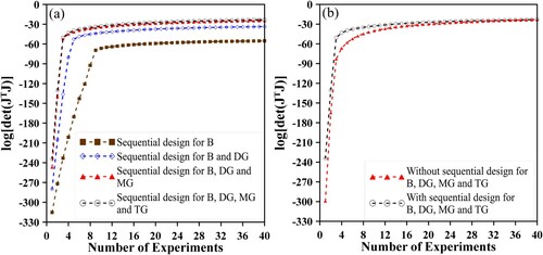
Figure 5(b) illustrates the gain in the determinant of ${\mathbf{J}}^{\text{T}}\mathbf{J}$ considering, or not, the sequential experimental design for the case where four species would be experimentally available. The red triangle curve represents the determinant of ${\mathbf{J}}^{\text{T}}\mathbf{J}$ taking into account the list of 40 candidates, of residence times, in an ascending order from 0.5–20 min, equally spaced of 0.5 min. And the black circle curve shows the increment observed in the determinant of ${\mathbf{J}}^{\text{T}}\mathbf{J}$ when the same number of cases (40 at total) was considered in a sorted sequence, derived from the sequential design procedure. It can be noticed that the sequential design improves values for the determinant of ${\mathbf{J}}^{\text{T}}\mathbf{J}$ up to the twentieth candidate, from that point and beyond there is no significant difference in the order of sub sequential candidates. For this reason, the inverse analysis from this point on was performed considering measures for the first 20 candidates indicated by the sequential experimental design: 5.5, 2.5, 18.5, 0.5, 1.5, 11, 4.5, 2, 20, 1, 6.5, 11.5, 4, 19.5, 3, 5, 10.5, 19, 3.5, and 6 min.

The synthetic experimental data were simulated from the accurate solution (GITT with NT = 40) evaluated in the 20 residence times mentioned before. At each residence time, the dimensionless average concentrations for the 4 species (TG, DG, MG and B) at the reactor outlet are obtained, totalling 80 synthetic experimental data. The exact solution was disturbed by a Gaussian noise with zero mean and a standard deviation $\sigma =\hat{\sigma }{\text{C}}^{\text{Sim}}$ in accordance with the following expression: (8) $\begin{array}{r}{\text{C}}^{\text{Exp}}={\text{C}}^{\text{Sim}}+\sigma N(0,1)\end{array}$(8)

Although lower values for $\hat{\sigma }$ were investigated, such as $\hat{\sigma }$ = 0.01 and $\hat{\sigma }$ = 0.03, only the results for $\hat{\sigma }$ = 0.05 will be here presented since such estimations have more discrepant values with respect to the original exact parameters.

Information about the approximation error in modelling is evaluated through a Monte Carlo simulation involving the difference between the accurate and approximate solutions,${\mathbf{C}}_{\text{Ac}}(\mathbf{p})-{\mathbf{C}}_{\text{Ap}}(\mathbf{p})$, for different vectors $\mathbf{p}$ randomly generated from uniform distributions. Table 3 presents the reference values and limits of the parameters considered in the sampling procedure used in the construction of information about the model error. Mean and standard deviation, for this approximation error, were calculated from this sampling and used in the approximate posterior formulation, Equation (6i), for those residence times chosen for the inverse analysis.

Table 3. Reference values and limits of the parameters $\kappa$ and $D$ considered in the sampling procedure in the error model approach.

Parameter	Exact value	Inferior limit	Superior limit
${\kappa }_1$	−5.35972	−5.62770	−5.09173
${\kappa }_2$	−5.01669	−5.26752	−4.76586
${\kappa }_3$	−4.72584	−4.96213	−4.48955
${\kappa }_4$	−3.96900	−4.16745	−3.77055
${\kappa }_5$	−4.67428	−4.90799	−4.44057
${\kappa }_6$	−6.04576	−6.34805	−5.74347
$D_{\text{TG}}$	−8.80134	−9.24141	−8.36128
$D_{\text{A}}$	−9.92738	−10.4238	−9.43101
$D_{\text{P}}$	−8.86012	−9.30313	−8.41711

It is also worth commenting that, in the sampling process, the variation of 5% in the parameters (in exponential format as here proposed) leads to a wide variation in the actual kinetic coefficient value higher than 37%. On the other hand, this variation on the kinetic coefficients may lead to more the 370% of variation on the dimensionless concentration for the species TG, DG, MG and B, as can be observed in Figure 6(a). These curves illustrate that 5% variation in the parameters is sufficient to create sampling curves (light grey curves) that cover a very wide region around the exact solution (solid black line). Figure 6(b) exemplifies the model error curves for the species TG evaluated by the difference between the GITT_NT=40 and GITT_NT=2, respectively, for an illustrative number of 200 samples of different vectors $\mathbf{p}$, and therefore 200 calculations of the difference between the accurate and approximate solutions. The number of samples, NS, must be evaluated to ensure a sampling which provides a fully converged value for the mean and standard deviation of the error. In this sense, Figure 6(c) shows the convergence analysis referring to the mean value of the error calculation between models for species TG, where it is noticed that a sampling with NS = 1000 is satisfactory to ensure, at this graphical scale, a converged behaviour to appropriately describe the mean of the error.

Figure 6. Error analysis. (6a) Sampling of error curves for TG with number of samples equal to 200, NS = 200; (6b) Convergence analysis for the mean of the error for TG with approximate solution by GITT_NT=2; (6c) Mean of the error for TG and B and (6d) for DG and MG with approximate solution by GITT_NT=2 and by CIEA.

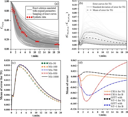
The same convergence analysis was performed for all other species for both approximate solutions, GITT_NT=2 and 1D-CIEA, even not being presented here. For all cases, the sampling number of NS = 1000 was suitable to perform the statistical analysis on the approximation error.

Figure 6(d) illustrate the converged mean of the error for the species TG and B generated for the GITT_NT=2 and 1D-CIEA, where it is possible to notice that the error profiles have behaviour completely distinct from those observed in the average concentration, but both GITT_NT=2 and 1D-CIEA error curves present similar tendency.

For all kinetic coefficients, a non-informative Uniform prior was assumed, while for the diffusion coefficients, a truncated Gaussian prior was considered with mean based on a correlation available in the literature [50] and standard deviation of 5%. For the priors’ range, for all parameters, a wide search interval for the MCMC was set as 50%, up and down, of the exact value of each parameter. Tables 4 to 7 present the result for the estimation of the parameters ‘κ‘ and ‘$D$‘ carried out with the approximate solutions, GITT_NT=2 and 1D-CIEA, respectively, considering 80 synthetic measurements with a deviation $\hat{\sigma }$ = 0.05 for the concentration of species TG, DG, MG and B evaluated in the 20 residence times indicated by the sequential experimental design. The MCMC was performed with an acceptance rate smaller than 50% for a total of 200000 accepted states. The parameter estimation was obtained through the calculation of the mean values and the quantiles of 99% for the credibility interval, both calculated from the accepted states after neglecting the burning period of 100000 states.

Table 4. Results for $\hat{\sigma }$ = 0.05 and credibility interval of 99% using the approximate solution from 3D GITT_NT=2 and the approximation error information.

			Total computational time^a: 4.32h
			Search step: 2.0 10^−3; Acceptance: 44.00%
Parameter	Initial guess	Exact value	Estimated	Minimum	Maximum	Error (%)
${\kappa }_1$	−2.67986	−5.35972	−5.23226	−5.40104	−4.94061	2.37800
${\kappa }_2$	−2.50834	−5.01669	−4.95242	−5.07705	−4.69741	1.28105
${\kappa }_3$	−2.36292	−4.72584	−4.37707	−4.80132	−4.02673	7.38011
${\kappa }_4$	−1.98450	−3.96900	−3.66313	−4.07241	−3.31520	7.70646
${\kappa }_5$	−2.33714	−4.67428	−4.61141	−4.69829	−4.51891	1.34496
${\kappa }_6$	−3.02288	−6.04576	−6.03114	−6.10960	−5.95595	0.24185
$D_{\text{TG}}$	−4.40067	−8.80134	−8.89102	−9.76302	−8.07658	1.01893
$D_{\text{A}}$	−4.96369	−9.92738	−10.27336	−11.21084	−9.85875	3.48511
$D_{\text{P}}$	−4.43006	−8.86012	−8.27231	−9.06810	−7.62360	6.63435

^a In a DESKTOP-T0TAGFG Intel(R) Core(TM) i7-7500U CPU @ 2.70 GHz 2.90 GHz with RAM of 8GB

Table 5. Results for $\hat{\sigma }$ = 0.05 and credibility interval of 99% using the approximate solution from 3D GITT_NT=2 without the approximation error information.

			Total computational time^a: 3.57h
			Search step: 2.0 10^−3; Acceptance: 47%
Parameter	Initial guess	Exact value	Estimated	Minimum	Maximum	Error (%)
${\kappa }_1$	−2.67986	−5.35972	−5.39955	−5.46939	−5.32628	0.74318
${\kappa }_2$	−2.50834	−5.01669	−5.06979	−5.13565	−5.00246	1.05847
${\kappa }_3$	−2.36292	−4.72584	−4.77795	−4.87654	−4.66998	1.10254
${\kappa }_4$	−1.98450	−3.96900	−4.03333	−4.12840	−3.91947	1.62101
${\kappa }_5$	−2.33714	−4.67428	−4.66791	−4.72480	−4.61061	0.13635
${\kappa }_6$	−3.02288	−6.04576	−6.02765	−6.08604	−5.97200	0.29951
$D_{\text{TG}}$	−4.40067	−8.80134	−8.80501	−9.23042	−8.03627	0.04171
$D_{\text{A}}$	−4.96369	−9.92738	−9.93274	−10.04956	−9.83064	0.05396
$D_{\text{P}}$	−4.43006	−8.86012	−8.17955	−8.45854	−7.79879	7.68125

^a In a DESKTOP-T0TAGFG Intel(R) Core(TM) i7-7500U CPU @ 2.70 GHz 2.90 GHz with RAM of 8GB

Tables 4 and 5 present the results obtained with the approximate solution GITT_NT=2, with and without taking into account the approximation error information in the estimation procedure, respectively. Similarly, Tables 6 and 7 present the results for the estimations obtained via 1D-CIEA, with and without, the approximation error information in the estimation procedure, respectively.

Table 6. Results for $\hat{\sigma }$ = 0.05 and credibility interval of 99% using the approximate solution from CIEA and the approximation error information.

			Total computational time^a: 1.71h
			Search step: 2.3 10^−3; Acceptance: 41%
Parameter	Initial guess	Exact value	Estimated	Minimum	Maximum	Error (%)
${\kappa }_1$	−2.67986	−5.35972	−5.29992	−5.40199	−5.20718	1.11559
${\kappa }_2$	−2.50834	−5.01669	−4.9868	−5.08809	−4.88792	0.59587
${\kappa }_3$	−2.36292	−4.72584	−4.51221	−4.76127	−4.3117	4.52044
${\kappa }_4$	−1.98450	−3.96900	−3.76492	−4.0118	−3.55905	5.14180
${\kappa }_5$	−2.33714	−4.67428	−4.6038	−4.6931	−4.50385	1.50771
${\kappa }_6$	−3.02288	−6.04576	−5.97438	−6.06365	−5.87371	1.18064
$D_{\text{A}}$	−4.96369	−9.92738	−10.0121	−10.0817	−9.93321	0.85320

^a In a DESKTOP-T0TAGFG Intel(R) Core(TM) i7-7500U CPU @ 2.70 GHz 2.90 GHz with RAM of 8GB.

Table 7. Results for $\hat{\sigma }$ = 0.05 and credibility interval of 99% using the approximate solution from CIEA without the approximation error information.

			Total computational time^a: 1.70h
			Search step: 1.5 10^–3; Acceptance: 35.4%
Parameter	Initial guess	Exact value	Estimated	Minimum	Maximum	Error (%)
${\kappa }_1$	−2.67986	−5.35972	−5.22998	−5.27678	−5.18624	2.42063
${\kappa }_2$	−2.50834	−5.01669	−4.97135	−5.02172	−4.92484	0.903698
${\kappa }_3$	−2.36292	−4.72584	−4.31178	−4.38817	−4.23931	8.76163
${\kappa }_4$	−1.9845	−3.96900	−3.62813	−3.71185	−3.54966	8.58831
${\kappa }_5$	−2.33714	−4.67428	−4.55212	−4.59894	−4.50604	2.61351
${\kappa }_6$	−3.02288	−6.04576	−5.96144	−6.01498	−5.90869	1.39464
$D_{\text{A}}$	−4.96369	−9.92738	−10.1184	−10.1516	−10.0843	1.92433

^a In a DESKTOP-T0TAGFG Intel(R) Core(TM) i7-7500U CPU @ 2.70 GHz 2.90 GHz with RAM of 8GB.

The estimated parameters for the situation where the approximation error information was taken into account presented a relative error lower than 7.70% with respect to the original exact values for kinetic and diffusion coefficients, and the credibility intervals are enveloping all exact reference values of them. Results for the estimation without taking into account the approximation error information for both approximate solutions (GITT_NT=2 and 1D-CIEA) present more expressive relative error such as 8% which suggests a poorer estimation, certainly due to the absence of the approximation error information. The credibility intervals from the estimation without the approximation error information does not include, for some parameters, their exact values and this seems like a deformation of the approximate posterior domain which led to less accurate estimations. These cases are illustrated in the Tables 5 and 7 in shaded form.

Figure 7 shows the evolution of the Markov chains of the parameters for the GITT_NT=2 approximate solution, evaluated with the approximation error information considering three different initial guesses: black curve for ${\mathbf{p}}^0=0.5{\mathbf{p}}_{\text{exact}}$; red curve for ${\mathbf{p}}^0=0.8{\mathbf{p}}_{\text{exact}}$; and blue curve for ${\mathbf{p}}^0=1.5{\mathbf{p}}_{\text{exact}}$. These results illustrate the convergence and agreement of the MCMC with approximation error model for different initial guesses, including those away from the exact value. Even for a wide range of initial guesses, the estimation converges to a region around the exact value of the parameters. It is also worth mentioning that a variation of 50% made in the initial guesses of the parameter, in the exponential format, represents a variation higher than 100% in the actual kinetic coefficients.

Figure 7. Markov chains for parameters obtained from approximate error approach through GITT_NT=2 assuming different initial guesses. Black curve: ${\mathbf{p}}^0=0.5{\mathbf{p}}_{\text{exact}}$; red curve: ${\mathbf{p}}^0=0.8{\mathbf{p}}_{\text{exact}}$; and Blue curve: ${\mathbf{p}}^0=1.5{\mathbf{p}}_{\text{exact}}$.

Figure 8 presents the final comparison for the original accurate result for the concentrations of all four measurable species. The obtained concentrations with the exact parameters via GITT_NT = 40 are presented as the black solid lines, the synthetic measurements with a standard deviation of $\hat{\sigma }$ = 0.05 are presented by the red symbols. The estimated concentrations, using the GITT_NT=2 solution in the inverse analysis, are presented by the blue stars with dashed line, and their respective credibility intervals of 99% are represented by the black dashed line.

Figure 8. Results for the synthetic data with $\hat{\sigma }$ = 0.05, estimated curves and their credibility intervals of 99% for (8a) triglyceride, (8b) biodiesel, (8c) diglyceride and (8d) monoglyceride.

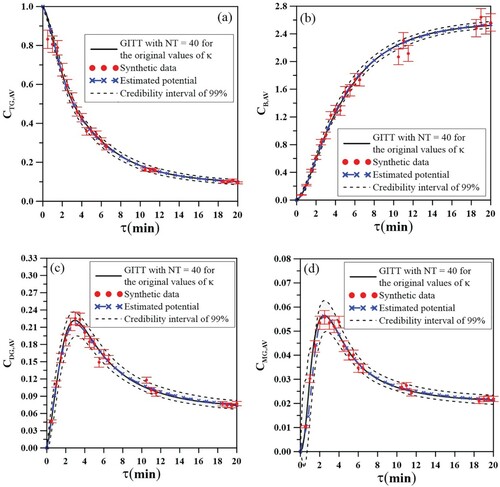
Once the equilibrium region in the iterative process of the MCMC is reached, after the burning period, the posterior prediction for each species was computed and stored for each state of MCMC, and from this posterior sample it was possible to calculate the mean and the quantiles of 99% to the estimated value of the concentration and its credibility interval. All estimated results show a good adherence to the experimental synthetic data recovering most of them, and in particular the agreement between the estimated curve and the exact one can be observed.

5. Conclusions

This work presents a methodology that allows to markedly reduce the computational effort in the estimation of the kinetic and diffusion coefficients for the transesterification reaction in microreactors, using approximate solutions and an information about the approximation error. The hybrid method GITT was used to construct an accurate solution for the forward problem governed by a multicomponent diffusive-convective-reactive nonlinear coupled 3D mathematical model, with sufficiently high truncation orders, such as NT = 40, while two approximate solutions were considered, one obtained by a 1D model reformulated via an improved lumped analysis (CIEA) and another one obtained from the 3D model itself solved by GITT but with low truncation order, as low as only two terms (NT = 2) in the eigenfunction expansion.

The ‘exact’ GITT solution (with a high truncation order, NT = 40) was used to perform the sensitivity analysis and the sequential experimental design for the problem, where it was possible to verify that the representation in exponential format for the kinetic and diffusion coefficients, $\text{k}={10}^{\kappa }$ and ${\text{D}}^{\ast }={10}^D$, instead of its original properties k and ${\text{D}}^{\ast }$, increases the sensitivity of the new parameters to be estimated as exponents (κ and D). From evaluating the $det({\mathbf{J}}^{\text{T}}\mathbf{J})$ it was indicated that replicating the experiments in the increasing order of the residence time proposed in a list of 40 different residence times as candidates, from 0.5 until 20 min with increment of 0.5 min, is not the best alternative to maximize $det({\mathbf{J}}^{\text{T}}\mathbf{J})$ and a sequence of 20 experiments collected and sorted from the original list of 40 candidates was presented and considered as the synthetic experimental measurements.

The approximation error information was obtained from a Monte Carlo simulation of the difference between the accurate and approximate solutions performed in a sampling generated from uniform distributions with means in the exact values of the parameters and 5%, for more and less, as interval limits. From a convergence analysis of the mean of the error, it was found a number of samples NS = 1000 as a satisfactory amount to represent the profile of the error representation along residence time.

The likelihood function was constructed using synthetic measurements with standard deviation of $\hat{\sigma }$ = 0.05 for the triglyceride, diglyceride, monoglyceride and biodiesel species, and the MCMC was employed using approximate solutions with and without their approximation error information. The estimation of the parameters in the exponential format ${10}^{\kappa }$ and ${10}^D$ were demonstrated for the case $\hat{\sigma }$ = 0.05 with relative errors lower than 8.0% compared to the exact values when the approximation error was considered. If this approximation is not considered, the error on estimative increases and a deformation in the credibility intervals occur and consequently the exact values are not recovered for all parameters. The computational time was fairly low, reaching as much as 1.71 and 4.72 h for CIEA and GITT_NT=2, respectively, in the microcomputer configuration adopted. The estimated potentials were recovered with strong adherence to the simulated data, which indicates that the combination of approximate solutions together with the information on approximation errors generates accurate results and fast algorithms for the inverse problem analysis.

Acknowledgements

The authors are grateful for the financial support offered by the Brazilian Government agencies CNPq, CAPES and FAPERJ.

Disclosure statement

No potential conflict of interest was reported by the author(s).

Additional information

Funding

The authors are grateful for the financial support offered by the Brazilian Government agencies: CNPq (National Council for Scientific and Technological Development), CAPES (Coordination for the Improvement of Higher Education Personnel), FAPERJ (Carlos Chagas Filho Foundation for Research Support in the State of Rio de Janeiro).

References

- Beck JV, Arnold KJ. Parameter estimation in engineering and science. New York: Wiley-Interscience; 1977.
- Alifanov OM. Inverse heat transfer problems. New York: Springer-Verlag; 1994.
- Migon HS, Gamerman D. Statistical inference: an integrated approach. London: Arnold; 1999.
- Özisik MN, Orlande HRB. Inverse heat transfer: fundamentals and applications. New York: Taylor & Francis; 2000.
- Kaipio J, Somersalo E. Statistical and computational inverse problems. Applied Mathematical Sciences, 160, Springer-Verlag New York; 2005.
- Gamerman D, Lopes HF. Markov chain Monte Carlo: stochastic simulation for Bayesian inference, 2nd ed., Boca Raton, FL,USA, Chapman & Hall/CRC; 2006.
- Schwaab M, Pinto JC. Optimum reference temperature for reparametrization of the Arrhenius equation. Part 1: problems involving one kinetic constant. Chem Eng Sci. 2007;62:2750–2764.
- Orlande HRB. (2015). Tutorial 7: the use of techniques within the Bayesian framework of statistics for the solution of inverse problem. Proc. of Metti 6 Advanced School: Thermal Measurements and Inverse Techniques, Biarritz, March 1-6.
- Nissinen A, Heikkinen L, Kaipio J. The Bayesian approximation error approach for electrical impedance tomography-experimental results. Meas. Sci. Tech. 2008;19:015501.
- Nissinen A, Heikkinen L, Kolehmainen V, et al. Compensation of errors due to discretization, domain truncation and unknown contact impedances in electrical impedance tomography. Meas. Sci. Tech. 2009;20:105504.
- Nissinen A, Heikkinen L, Kaipio J. Compensation of modeling errors due to unknown boundary domain in electrical impedance tomography. IEEE Trans. Med. Im. 2011a;30:231–242.
- Nissinen A, Heikkinen L, Kaipio J. Reconstruction of domain boundary and conductivity in electrical impedance tomography using the approximation error approach. Int. J. Uncertainty Quant. 2011b;1:203–222.
- Lamien B, Orlande HRB. (2013). Approximation error model to account for convective effects in liquids characterized by the line heat source probe. In: Proc. IPDO-2013 4th Inverse Problems, Design and Optimization Symposium, Albi, França, Jun 26-28.
- Orlande HRB, Dulikravich GS, Neumayer M, et al. Accelerated Bayesian inference for the estimation of spatially varying heat flux in a heat conduction problem. Numerical Heat Transfer, Part A: Applications: An International Journal of Computation and Methodology. 2014;65(1):1–25.
- Pacheco CC, Orlande HRB, Colaço MJ, et al. Estimation of a location- and time-dependent high-magnitude heat flux in a heat conduction problem using the Kalman Filter and the approximation error model. Numerical Heat Transfer. Part A, Applications. 2015;68:1198–1219.
- Lamien B, Orlande HRB, Eliçabe GE. Particle filter and approximation error model for state estimation in Hyperthermia. J Heat Transfer. 2017;139:012001.
- Lamien B, Le Maux D, Courtois M, et al. A Bayesian approach for the estimation of the thermal diffusivity of aerodynamically levitated solid metals at high temperatures. Int J Heat Mass Transf. 2019;141:265–281.
- Aperecido JB, Cotta RM, Özişik MN. Analytical solutions to two-dimensional diffusion type problems in irregular geometries. J Franklin Inst. 1989;326(3):421–434. doi:https://doi.org/10.1016/0016-0032(89)90021-5.
- Cotta RM. Hybrid numerical-analytical approach to nonlinear diffusion problems. Num. Heat Transfer Part B. 1990;127:217–226.
- Cotta RM. Integral transforms in computational heat and fluid flow. Boca Raton (FL): CRC Press; 1993.
- Cotta RM. Benchmark results in computational heat and fluid flow: the integral transform method. Int J Heat Mass Transfer. 1994;37:381–393.
- Cotta RM. The integral transform method in thermal & fluids sciences & engineering. New York: Begell House; 1998.
- Cotta RM, Mikhailov MD. Heat conduction: lumped analysis, integral transforms, symbolic computation. Chichester: Wiley-Interscience; 1997.
- Cotta RM, Mikhailov MD. Hybrid methods and symbolic computations. In: WJ Minkowycz, EM Sparrow, JY Murthy, editors. Handbook of numerical heat transfer, 2nd ed., Chapter 16. New York: John Wiley; 2006. p. 493–522.
- Cotta RM, Knupp DC, Naveira-Cotta CP, et al. Unified integral transforms algorithm for solving multidimensional nonlinear convection-diffusion problems. Numerical Heat Transfer, Part A: Applications: An Int. J. Computation Methodology. 2013;63(11):840–866.
- Cotta R M, Naveira-Cotta C P, Knupp D C. Nonlinear eigenfunction expansions for the solution of nonlinear diffusion problems. Proc. of 1st Thermal and Fluid Engineering Summer Conference, TFESC. 2015-08: 9–12
- Cotta RM, Knupp DC, Naveira-Cotta CP. Analytical heat and fluid flow in microchannels and microsystems, Mechanical Engineering Series. New York: Springer; 2016a.
- Cotta RM, Naveira-Cotta CP, Knupp DC. Nonlinear eigenvalue problem in the integral transforms solution of convection-diffusion with nonlinear boundary condition. Int. Journal of Numerical Methods for Heat and Fluid Flow. 2016b;26(3&4):767–789.
- Cotta RM, Knupp DC, Quaresma JNN, et al. Analytical methods in heat transfer. In: FA Kulacki, editor. Handbook of thermal science and engineering. Springer International Publishing, Cham-Switzerland; 2018a, Chapter 2, p. 61–126.
- Cotta RM, Naveira-Cotta CP, Knupp DC, et al. Recent advances in computational-analytical integral transforms for convection-diffusion problems. Heat & Mass Transfer. Invited Paper, 2018b;54:2475–2496.
- Pontes P C, Almeida A P, Naveira-Cotta C P, etal. Analysis of Mass Transfer in Hollow-Fiber Membrane Separator via Nonlinear Eigenfunction Expansions, Multiphase Science and Technology, v. 30. 2019: 165–186
- Serfaty R, Cotta RM. Integral transform solutions of diffusion problems with nonlinear equation coefficients. Int. Comm. Heat & Mass Transfer. 1990;17(6):851–864.
- Mikhailov MD, Özisik MN. Unified analysis and solution in heat and mass diffusion. New York: Wiley; 1984; also, Dover Publications, 1994.
- Özisik MN. Heat conduction. 2nd ed. New York: John Wiley & Sons; 1993.
- Naveira-Cotta CP, Orlande HRB, Cotta RM. Integral transforms and Bayesian inference in the identification of variable thermal conductivity in two-phase dispersed systems. Numerical Heat Transfer. Part B, Fundamentals. 2010a;57:173–202.
- Naveira-Cotta CP, Cotta RM, Orlande HRB. Inverse analysis of forced convection in micro-channels with slip flow via integral transforms and Bayesian inference. Int J Therm Sci. 2010b;49:879–888.
- Naveira-Cotta CP, Cotta RM, Orlande HRB. Inverse analysis with integral transformed temperature fields: Identification of thermophysical properties in heterogeneous media. Int J Heat Mass Transf. 2011a;54:1506–1519.
- Naveira-Cotta CP, Orlande HRB, Cotta RM. Combining integral transforms and Bayesian inference in the simultaneous identification of variable thermal conductivity and thermal capacity in heterogeneous media. J Heat Transfer. 2011b;133:111301.
- Knupp DC, Naveira-Cotta CP, Ayres JVC, et al. Theoretical-experimental analysis of heat transfer in nonhomogeneous solids via improved lumped formulation, integral transforms and infrared thermography. Int. J. Thermal Sciences. 2012a;62:71–84.
- Knupp DC, Naveira-Cotta CP, Ayres JVC, et al. Space-variable thermophysical properties identification in nanocomposites via integral transforms, Bayesian inference and infrared thermography. Inverse Problems in Science & Eng. 2012b;20(5):609–637.
- Knupp DC, Naveira-Cotta CP, Orlande HRB, et al. Experimental identification of thermophysical properties in heterogeneous materials with integral transformation of temperature measurements from infrared thermography. Exp. Heat Transfer. 2013;26:1–25.
- Abreu LA, Orlande HRB, Kaipio J, et al. Identification of contact failures in multi-layered composites with the Markov chain Monte Carlo method. ASME J. Heat Transfer. 2014;136(10):101302–101311.
- Abreu LAS, Orlande HRB, Colaço MJ, et al. Detection of contact failures with the Markov chain Monte Carlo method by using integral transformed measurements. Int. J. Thermal Sciences. 2018;132:486–497.
- Aparecido JB, Cotta RM. Modified one-dimensional fin solutions. Heat Transf. Eng. 1989;11:49–59.
- Regis CR, Cotta RM, Su J. Improved lumped analysis of transient heat conduction in a nuclear fuel rod. Int Commun Heat Mass Transfer. 2000;27:357–366.
- Naveira CP, Lachi M, Cotta RM, et al. Hybrid formulation and solution for transient conjugated conduction external convection. Int. J. Heat & Mass Transfer. 2009;52(1-2):112–123.
- Sphaier LA, Su J, Cotta RM, et al. Macroscopic heat conduction formulation. In: FA Kulacki et al., editor. Handbook of thermal science and engineering, Chapter 1. Springer International Publishing, Cham/Switzerland; 2018. p. 3–59.
- Kakaç S, Yener Y, Naveira-Cotta CP. Heat conduction. 5th ed., CCR Press, Taylor and Francis, New York; 2018. ISBN 9781138943841
- Costa Junior JM, Naveira-Cotta CP. Estimation of kinetic constants in micro reactors for biodiesel synthesis: Bayesian inference with reduced mass transfer model. Chem Eng Res Des. 2019;141:550–565.
- Al-Dhubabian AA. (2005). Production of biodiesel from Soybean Oil in a micro scale reactor, Thesis (M.Sc.), Oregon State University, Corvallis, OR, USA.
- Guan G, Kusakabe K, Moriyama K, et al. Transesterification of sunflower oil with methanol in a microtube reactors. Ind Eng Chem Res 2009;48:1357–1363.
- Guan G, Teshima M, Sato C, et al. Two-phase flow behavior in microtube reactors during biodiesel production from waste cooking oil. AIChE J. 2010;56(5):1383–1390.
- Xie T, Zhang L, Xu N. Biodiesel synthesis in microreactors. Green Process Synth. 2012;1:61–70.
- Billo RE, Oliver CR, Charoenwat R, et al. A cellular manufacturing process for a full-scale biodiesel microreactor. J Manuf Syst. 2015;37(Part 1):409–416.
- Pontes PC, Naveira-Cotta CP, Quaresma JNN. Three-dimensional reaction-convection-diffusion analysis with temperature influence for biodiesel synthesis in micro-reactors. Int J Therm Sci. 2017;118:104–122.
- Noureddini H, Zhu D. Kinetics of transesterification of soybean Oil. Journal of the American Oil Chemist's Society. 1997;74(11):1457–1463.
- Meher LC, Vidya Sagar D, Naik SN. Technical aspects of biodiesel production by transesterification – a review. Renewable Sustainable Energy Rev. 2006;10:248–268.
- Dennis BH, Jin W, Cho J, et al. Inverse determination of kinetic rate constants for transesterification of vegetable oils. Inverse Probl Sci Eng. 2008;16(6):693–704.
- Malengier B, Tamalapakula JL, Pushpavanam S. Comparison of laminar and plug flow-fields on extraction performance in micro-channels. J Micromech Microeng. 2012;21:115030–115042.
- De Boer K, Bahri PA. (2009). Investigation of liquid-liquid two phase in biodiesel production. Seventh International Conference on CFD in the Minerals and Process Industries, Melbourne, Australia, December 9-11.
- Richard R, Thiebaud-Roux S, Prat L. Modelling the kinetics of transesterification reaction os sunflower oil with ethanol in microreactors. Chem Eng Sci. 2013;87:258–269.
- Pontes PC, Chen K, Naveira-Cotta CP, et al. Mass transfer simulation of biodiesel synthesis in microreactors. Comput Chem Eng. 2016;93:36–51.
- Costa Junior JM, Naveira-Cotta CP, Moraes DB, et al. Innovative metallic microfluidic device for intensified biodiesel production. Industrial and Engineering. Chemistry Research. 2020a;59:389–398.
- Costa Junior JM, Pontes PC, Naveira-Cotta CP, et al. A hybrid approach to probe microscale transport phenomena: application to biodiesel synthesis in micro-reactors. In: AK Gupta, editor. Innovations in sustainable energy and cleaner environment, Chapter 20. Springer-Verlag; 2020b. p. 457–486. ISBN: 978-981-13-9012-8.
- Pinto JC, Lobão MW, Monteiro JL. Sequential experimental design for parameter estimation: a different approach. Chem Eng Sci. 1990;45(4):883–892.
- Pinto JC, Lobão MW, Monteiro JL. Sequential experimental design for parameter estimation: analysis of relative deviations. Chem Eng Sci. 1991;46(12):3129–3138.
- Orlande H R B, Colaço M J, Dulikravich G S. Approximation of the likelihood function in the bayesian technique for the solution of inverse problems. Proc. of the Inverse Problems, Design and Optimization Symposium. 2007;4:16–18.
- Wolfram S. The Mathematica book. Wolfram Media, Champaign Illinois, USA; 2016.