Simultaneous reconstruction of optical absorption property and speed of sound in intravascular photoacoustic tomography

Abstract

Intravascular photoacoustic tomography (IVPAT) is a newly developed imaging modality for the diagnosis and intervention of coronary artery diseases. It is an ill-posed nonlinear least squares (NLS) problem to recover the absorbed optical energy density (AOED) and optical absorption coefficient (OAC) distribution in the vascular cross sections from pressure photoacoustically generated by tissues with variable speed of sound (SoS). The prior knowledge of the SoS is usually unavailable before IVPAT scanning. The ideal assumption of a constant SoS leads to degraded image quality. This paper focuses on improvement of image quality for IVPAT in tissues with variable SoS by simultaneously recovering the SoS, AOED and OAC from the measured time-dependent pressure series. The joint recovery is implemented by alternately minimizing the errors between the measured and theoretical pressure by forward simulation. The demonstration results indicate that the normalized mean square absolute distance (NMSAD) of the reconstructions produced by this method is decreased by about 15% in comparison to that of the reconstructions with a fixed SoS. Comparison results show that this method outperforms the delay compensation method in recovering the AOED and the two-step algorithm in estimating the OAC by about 20% and 25% in NMSAD respectively.

KEYWORDS:

• Intravascular photoacoustic tomography (IVPAT)
• image reconstruction
• absorbed optical energy density (AOED)
• optical absorption coefficient (OAC)
• speed of sound (SoS)

AMS/MSC:

• 35R30
• 65R32
• 35L05
• 65M32

1. Introduction

1.1. Backgrounds

Intravascular photoacoustic tomography (IVPAT) is a minimally invasive imaging modality for the visualization of coronary atherosclerosis and guidance of interventional treatment of cardiovascular atherosclerotic diseases by combing photoacoustic tomography (PAT) with endoscopic detection. It is a powerful tool complementary to intravascular ultrasound (IVUS) [1]. A cardiac catheter with a special tiny probe mounted on its tip is directly inserted into the target vascular lumen and is pushed to the distal end. The probe integrates multimode optical fibre, optical reflective elements and miniature ultrasonic transducers. During the pullback of the catheter, the probe circumferentially scans the surrounding tissue and collects ultrasonic waves which are photoacoustically generated by tissues [2]. The images of the initial acoustic pressure or absorbed optical energy density (AOED) distribution in the vascular cross-sections are reconstructed from the measured time series of acoustic pressure by solving the acoustic inverse problem [3]. Further, the spatial distribution of the optical absorption coefficient (OAC), scattering coefficient and thermal expansion coefficient is recovered from the optical absorption by using a two-step algorithm to implement quantitative IVPAT (qIVPAT) [4]. The images present the morphological structures and functional components of arterial vessels which are of significance for accurate identification and characterization of atherosclerotic plaques [5].

To simplify the ill-posed problem of PAT image reconstruction, many methods assume a constant speed of ultrasound propagating in tissues to be imaged [6]. Experimental results have shown that such an ideal premise is reasonable only if the variations in the speed of sound (SoS) are small or the imaging target is small enough relative to the scanning geometry [7]. For those imaging objects with a large size or significantly changing SoS, the images reconstructed based on a constant SoS will contain severe distortions, artifacts, and blurring, especially around the boundaries and the tangent direction of the target. This ideal premise is also invalid in IVPAT reconstructions because the changes in the SoS of human soft tissues can reach up to 10% [8].

1.2. Related work

Many methods have been proposed to reduce the influence of the variable SoS on PAT image reconstruction such as time-reversal (TR) method [9], Neumann-series based algorithm [10] and iterative method [11], etc. These methods compensate for the errors in the measured pressure caused by the variable SoS through introducing the prior knowledge of the SoS distribution into image reconstruction. However, this prior knowledge is usually unavailable or is difficult to be accurately measured prior to PAT scanning in most practical applications.

Several approaches which do not need such prior knowledge have also been developed including full-wave iterative method [12], correlation-based method [13], autofocus approach [14,15], optimal SoS group [16] and delay compensation [17], etc. The full-wave iteration is sensitive to the possible noise in the acoustic measurements. Moreover, its high computation cost in achieving reconstructions with satisfied quality limits its real-time application. The correlation-based method requires the imaging object to be small enough and the receiving probe to be far away from the object. The autofocus approach needs the prior knowledge about the rough location of the object. A too small region of interest may lead to the increased computation burden. The accuracy of the optimal SoS group method highly depends on the initial group of the SoS which is usually obtained according to the prior knowledge about the internal structures of the object. Hence, it is more suitable for photoacoustic-ultrasonic (PAUS) dual-modal imaging instead of single-modal PAT. The delay compensation method also needs a properly selected initial SoS, and it takes a relatively long time to reconstruct a single image in comparison to other methods.

Theoretically, the images reconstructed based on the known SoS distribution have higher quality than those reconstructed with a constant SoS or by compensating for the variable SoS. Ultrasonic transmission tomography (UTT) is usually utilized to measure the SoS distribution in the imaging object prior to the photoacoustic (PA) scanning [18]. However, it is not applicable to IVPAT because of the prolonged interventional imaging process with an additional device.

An alternative method is to simultaneously reconstruct the SoS and the optical absorption distribution from the PA measurements. For example, Yuan et al. [19,20] presented a nonlinear iterative algorithm based on finite element analysis (FEA). They solved the Helmholtz wave equation which satisfies the second-order absorbing boundary condition for acoustically inhomogeneous medium after finite element discretization to obtain the theoretical initial pressure. Then, they solved the problem of minimizing the root mean square error of the measured and the theoretical pressure to reconstruct the images of the SoS and the optical absorption distribution. The FEA-based algorithms usually have high computation cost due to complex and repeated calculations, especially in the case of fine grids. In addition, the accuracy of the solutions highly depends on the boundary conditions. The usually adopted boundary conditions are summarized as two categories. The first simple one is to set the boundary values of the variables to be solved. It is only applicable to the solution domain with a regular shape such as ball or circle. The second one is to specify the directional derivative of the normal outside the target boundary. It has no strict requirements for the shape of the solution domain. But, its computational complexity is higher than the first one because of the repeated calculation of the average curvature and Gaussian curvature on the solution domain surface.

Zhang et al. [21] proposed a time-domain iterative approach by Radon-transforming the error function relating to the imaging model. They first reconstructed the SoS distribution by using an iterative gradient-based algorithm on the premise of the unchanged optical absorption. Then, they reconstructed the optical absorption distribution based on the recovered SoS by combining a multi-directional search algorithm with the standard conjugate gradient algorithm. This approach makes full use of the redundancy in the PA measurements and reduces the accuracy requirement of the error function gradient. However, it is only suitable for those imaging objects with low acoustic scattering because of the use of Radon transform. In IVPAT imaging, the acoustic inhomogeneity of the vessel wall, atherosclerotic plaques and other lesions leads to reflection and scattering of the acoustic waves, especially at the severely mismatched tissue boundaries such as vascular lumen. Later, Huang et al. [22-24] improved the joint reconstruction (JR) method by solving two penalty least squares problems alternately. They also investigated the numerical properties of the JR problem to provide insights into the practical feasibility of JR. Their method has been demonstrated on PAT systems equipped with a detector scanning around the object to acquire pressure data. However, it cannot be directly applied to IVPAT because the technique used to reconstruct images relates to the way upon acquiring acoustic pressure, while the intravascular photoacoustic signal acquisition is highly limited caused by the special scanning aperture enclosed in a closed vascular lumen [25].

1.3. Objective of this work

The primary contribution of this work is to present a novel approach to improve image quality for IVPAT in tissues with the variable SoS by simultaneously recovering the spatial distribution of AOED, OAC and SoS in vascular cross-sections from intravascular PA measurements. The demonstration experiments were conducted and the reconstruction quality were quantitatively evaluated. Experiments that revealed the dependence of the reconstruction quality on the initial plan and iteration step size were also conducted. Additionally, the reconstructions provided by using a fixed SoS and the proposed method were compared. Comparison experiments between the AOED estimation with our method and the delay compensation method [17] as well as the OAC estimation with our method and the two-step qIVPAT algorithm [4] were also provided.

The paper is organized as follows. Section 2 describes the proposed approach in detail. Section 3 presents the demonstration results. Related discussions are given in Section 4 and the paper concludes with a summary in Section 5.

2. Method

2.1. Forward simulation

2.1.1. Description of IVPAT forward problem

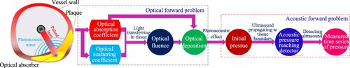
As illustrated in Figure 1, the forward problem of IVPAT includes an optical problem and an acoustic problem [26]. The optical problem describes the transmission of short laser pulses in tissues. The AOED at the position r in the imaging region Ω is determined by (1) $A(\mathbf{\text{r}},\lambda )={\mu }_{\text{a}}(\mathbf{\text{r}},\lambda )\Phi (\mathbf{\text{r}},\lambda ;{\mu }_{\text{a}}(\mathbf{\text{r}},\lambda ),{\mu }_{\text{s}}(\mathbf{\text{r}},\lambda )),$(1) where $\mathbf{\text{r}}\in \mathrm{\Omega }$, Ω is a bounded domain, λ is the wavelength of the incident light, A(r, λ) is the AOED at r, Φ is the optical radiance energy, and μ_a(r, λ) and μ_s(r, λ) are, respectively, the OAC and scattering coefficient at r. Partial light absorbed by the tissues is transformed into ultrasonic waves by the biological PA effect. The initial acoustic pressure is obtained by (2) $p_0(\mathbf{\text{r}},\lambda )=\Gamma (\mathbf{\text{r}},\lambda )A(\mathbf{\text{r}},\lambda ),$(2) where p₀(r, λ) is the initial acoustic pressure at r and Γ(r, λ) represents the PA conversion efficiency, i.e. the conversion efficiency of the absorbed optical energy relative to the PA wave. It depicts the thermodynamic properties of the tissues and can be expressed by Gruneisen coefficient.

Figure 1. Block diagram of IVPAT.

2.1.2. Optical simulation based on radiative transfer equation

In this study, we model the light transportation in tissues by the radiative transfer equation (RTE). The time-independent steady state RTE is written as [27,28] (3) $Q(\mathbf{\text{r}},\hat{s})-[\hat{s}\cdot \mathrm{\nabla }+{\mu }_{\text{a}}(\mathbf{\text{r}})+{\mu }_{\text{s}}(\mathbf{\text{r}})]\phi (\mathbf{\text{r}},\hat{s})+{\mu }_{\text{s}}(\mathbf{\text{r}}){\oint }_{S^{n-1}}\Theta (\hat{s},{\hat{s}}^{\mathrm{\prime }})\phi (\mathbf{\text{r}},{\hat{s}}^{\mathrm{\prime }})\text{d}{\hat{s}}^{\mathrm{\prime }}=0,$(3) where $\phi (\mathbf{\text{r}},\hat{s})$ denotes the optical radiation energy at r per unit area along the direction $\hat{s}\in {\hat{S}}^{n-1}$_, ${\hat{s}}^{n-1}$ is the angular space of n–1 dimension, $\Theta (\hat{s},{\hat{s}}^{\mathrm{\prime }})$ represents the Henyey-Greenstein scattering phase function indicating the probability that a scattered photon originally travelling in direction $\hat{s}$ ends up travelling in direction ${\hat{s}}^{\mathrm{\prime }}$, and $Q(\mathbf{\text{r}},\hat{s})$ is a light source.

RTE is simplified as a diffusion equation (DE) in the case of µ_a<<µ_s′, where µ_s′ is the reduced scattering coefficient, (4) ${{\mu }_{\text{s}}}^{\mathrm{\prime }}={\mu }_{\text{s}}(1-g),$(4) and g is the anisotropy factor. The time-independent DE satisfying the Robin boundary condition is expressed as (5) $-\mathrm{\nabla }\cdot \left\{\frac{\mathrm{\nabla }\Phi (\mathbf{\text{r}})}{3[{\mu }_{\text{a}}(\mathbf{\text{r}})+{{\mu }_{\text{s}}}^{\mathrm{\prime }}(\mathbf{\text{r}})]}\right\}+{\mu }_{\text{a}}(\mathbf{\text{r}})\Phi (\mathbf{\text{r}})=Q(\mathbf{\text{r}}),$(5) where Q(r) is the source term. Then, the AOED is obtained by (6) $A(\mathbf{\text{r}})={\mu }_{\text{a}}(\mathbf{\text{r}})\Phi (\mathbf{\text{r}}).$(6)

2.1.3. Acoustic simulation based on finite-difference time-domain

The propagation of the photoacoustically generated ultrasonic wave in tissues satisfies the PA wave equation [26], (7) ${\mathrm{\nabla }}^{2}p(\mathbf{\text{r}},t)-\frac{1}{{[c(\mathbf{\text{r}})]}^2}\frac{{\mathrm{\partial }}^2}{\mathrm{\partial }{t}^2}p(\mathbf{\text{r}},t)=-A(\mathbf{\text{r}})\frac{\beta }{C_p}I(t),$(7) where $\mathrm{\nabla }$ is Hamilton operator, p(r, t) denotes the pressure at the location r and time t, c(r) is the SoS at r, A(r) is the AOED at r, β is the isobaric thermal expansion coefficient, C_p is the specific heat capacity, and I(t) is the temporal function representing the instantaneous incident laser pulse.

The acoustic vibration satisfies Newton's second law, the law of conservation of mass and the equation of state which describes the relationship between the state parameters including acoustic pressure, temperature and volume. According to these basic laws, the coupled equations of motion, continuity and state regarding the acoustic pressure p, the particle velocity v, and the medium density ρ are derived [29], (8) $\{\begin{array}{l}\rho {\displaystyle \frac{\mathrm{\partial }v}{\mathrm{\partial }t}}=-\mathrm{\nabla }p\\ {\displaystyle \frac{\mathrm{\partial }{\rho }^{\mathrm{\prime }}}{\mathrm{\partial }t}}=-\mathrm{\nabla }\cdot (\rho \mathit{v})\\ p=v^2{\rho }^{\mathrm{\prime }}\end{array},$(8) where ρ′ is the variation in the tissue density. By combining Equations (7) and (8), we obtain (9) $\{\begin{array}{l}{\displaystyle \frac{\mathrm{\partial }p}{\mathrm{\partial }t}}=-\rho .c^2\left({\displaystyle \frac{\mathrm{\partial }{v}_{\theta }}{\mathrm{\partial }\theta }}+{\displaystyle \frac{\mathrm{\partial }{v}_l}{\mathrm{\partial }l}}\right)+{\displaystyle \frac{\beta .c^2}{C_p}}A(r).I(t)\\ {\displaystyle \frac{\mathrm{\partial }{v}_{\theta }}{\mathrm{\partial }t}}=-{\displaystyle \frac{1}{\rho }}{\displaystyle \frac{\mathrm{\partial }p}{\mathrm{\partial }\theta }}\\ {\displaystyle \frac{\mathrm{\partial }{v}_l}{\mathrm{\partial }t}}=-{\displaystyle \frac{1}{\rho }}{\displaystyle \frac{\mathrm{\partial }p}{\mathrm{\partial }l}}\end{array},$(9) where v_θ and v_l are the particle velocity along θ-axis and l-axis of the θ-l polar coordinate system respectively. Then, Equation (9) is discretized by using the finite-difference time-domain (FDTD) algorithm as follows, (10) $\{\begin{array}{l}{p}^{(n+1)}(j,k)=p^{(n)}(j,k)-\rho \cdot [c(j,k){]}^2\cdot \mathrm{\Delta }t\\ \cdot \{{\displaystyle \frac{1}{\mathrm{\Delta }\theta }}\left[v_{\theta }^{(n+(1/2))}(j+{\displaystyle \frac{1}{2}},k)-v_{\theta }^{(n+(1/2))}(j-{\displaystyle \frac{1}{2}},k)\right]\\ \begin{array}{cc}\begin{array}{cc}& \end{array}& \end{array}+{\displaystyle \frac{1}{\mathrm{\Delta }l}}\left[v_l^{(n+(1/2))}(j,k+{\displaystyle \frac{1}{2}})-v_l^{(n+(1/2))}(j,k-{\displaystyle \frac{1}{2}})\right]\}+{\displaystyle \frac{\beta \cdot {[c(j,k)]}^2\cdot \mathrm{\Delta }t}{C_P}}A(j,k)\cdot I^{(n)}\\ v_{\theta }^{(n+(1/2))}(j-{\displaystyle \frac{1}{2}},k)=v_{\theta }^{(n-(1/2))}(j-{\displaystyle \frac{1}{2}},k)-{\displaystyle \frac{\mathrm{\Delta }t}{\rho \cdot \mathrm{\Delta }\theta }}[p^{(n)}(j,k)-p^{(n)}(j-1,k)]\\ v_l^{(n+(1/2))}(j,k-{\displaystyle \frac{1}{2}})=v_l^{(n-(1/2))}(j,k-{\displaystyle \frac{1}{2}})-{\displaystyle \frac{\mathrm{\Delta }t}{\rho \cdot \mathrm{\Delta }l}}[p^{(n)}(j,k)-p^{(n)}(j,k-1)]\end{array},$(10) where (j, k) is the polar coordinate of the location r in the θ-l polar coordinate system, Δθ and Δl are the unit lengths of θ-axis and l-axis respectively, Δt is the discrete time interval, n is the discrete time, p⁽ⁿ⁾(j, k) is the acoustic pressure at the location (j, k) and time n, c(j, k) is the SoS at (j, k), A(j, k) is the AOED at (j, k), $v_{\theta }^{(n+(1/2))}(j,k)$ is the particle velocity at the location (j, k) and time $n+(1/2)$ along θ-axis, $v_l^{(n+(1/2))}(j,k)$ is the particle velocity at the location (j, k) and time $n+(1/2)$ along l-axis, and I⁽ⁿ⁾ is the intensity of the incident laser pulse at time n.

The theoretical acoustic pressure distribution in a vascular cross-section is achieved by solving Equation (10) where the AOED is obtained by optical simulation as described in Section 2.1.2.

2.2. Simultaneous reconstruction of AOED and SoS

2.2.1. Reconstruction of AOED

We assume that the influences of the acoustic attenuation and the spatial impulse response (SIR) and electrical impulse response (EIR) of the detector on the signal acquisition are ignored. The AOED for the given SoS is determined by (11) $\hat{A}(\mathbf{\text{r}})=\underset{A\ge 0}{\arg min}[\Vert p_{\text{e}}(\mathbf{\text{r}},A(\mathbf{\text{r}}),c(\mathbf{\text{r}}))-p_{\text{m}}(\mathbf{\text{r}}){\Vert }^2+\lambda {\mathrm{\Phi }}_{\text{TV}}(A(\mathit{r}))],$(11) where $\hat{A}(\mathbf{\text{r}})$ is the estimated AOED at r, A(r) is the AOED to be optimized, c(r) is the SoS at r, p_m(r) is the measured acoustic pressure at r, and p_e(r, A(r), c(r)) is the theoretical acoustic pressure at r regarding A(r) and c(r), $\Vert \cdot \Vert$denotes the Euclidean norm, λ is the regularization parameter, and ${\mathrm{\Phi }}_{\text{TV}}(A(\mathit{r}))$ is the term of total variation (TV) regularization, (12) ${\mathrm{\Phi }}_{\text{TV}}(A(\mathit{r}))=\sqrt{\Vert \mathbf{\text{L}}A(\mathbf{\text{r}}){\Vert }_1^2+\eta }.$(12)

Here, η > 0 is a constant, $\Vert \cdot {\Vert }_1$denotes the l1 norm, and L is the difference matrix [30], $L=\left[\begin{array}{cccc}1& -1& & \\ & 1& -1& \\ & & \ddots & \ddots \\ & & 1& -1\end{array}\right]$

We choose TV-regularizer instead of standard Tikhonov-regularizer because of the diversity of the complicated multi-layered structures of coronary vessel wall including plaques and the over-smoothing of standard Tikhonov-regularizer which results in the loss of target details in the reconstructed images [23,31].

Equation (11) is iteratively solved by generating A_k+1 via (13) $A_{k+1}(\mathbf{\text{r}})=A_k(\mathbf{\text{r}})-{\mathbf{\text{W}}}^{-1}(A_k(\mathbf{\text{r}}))\{{\mathit{H}}^T(c_k(\mathbf{\text{r}}))[\mathit{H}(c_k(\mathbf{\text{r}}))A_k(\mathbf{\text{r}})-p_{\text{m}}(\mathbf{\text{r}})]+\lambda {\mathbf{\text{L}}}_{\eta }(A_k(\mathbf{\text{r}}))A_k(\mathbf{\text{r}})\},$(13) where A_k(r) and c_k(r) are the AOED and SoS at r after k-th iteration respectively, H(c_k(r)) is an imaging operator regarding c_k(r), (14) $\mathit{H}(c_k(\mathbf{\text{r}}))A_k(\mathbf{\text{r}})=p_{\text{e}}(\mathbf{\text{r}},A(\mathbf{\text{r}}),c_k(\mathbf{\text{r}})),$(14)

W is the Hessian matrix, (15) $\mathbf{\text{W}}(A_k(\mathbf{\text{r}}))={\mathit{H}}^T(c_k(\mathbf{\text{r}}))\mathit{H}(c_k(\mathbf{\text{r}}))+\lambda {\mathbf{\text{L}}}_{\eta }(A_k(\mathbf{\text{r}})),$(15) and (16) ${\mathbf{\text{L}}}_{\eta }(A_k(\mathbf{\text{r}}))={\mathbf{\text{L}}}^T[diag(\sqrt{\Vert \mathbf{\text{L}}{A}_k(\mathbf{\text{r}}){\Vert }_1^2+\eta }){]}^{-1}\mathbf{\text{L}}.$(16)

2.2.2. Reconstruction of SoS

The SoS for the given AOED is determined by (17) $\hat{c}(\mathbf{\text{r}})=\underset{c\ge 0}{\arg min}[\Vert p_{\text{e}}(\mathbf{\text{r}},A(\mathbf{\text{r}}),c(\mathbf{\text{r}}))-p_{\text{m}}(\mathbf{\text{r}}){\Vert }^2+\alpha \Vert c(\mathit{r}){\Vert }_1^{(1/2)}],$(17) where $\hat{c}(\mathbf{\text{r}})$ is the estimated SoS at r, c(r) is the SoS to be optimized, and α > 0 is the regularizing parameter.

The regularizers in Equations (11) and (17) are chosen depending on the magnitude of the AOED and SoS. The SoS of vessel wall tissues ranging from 1400 m/s to 1650 m/s is far larger than the AOED which is usually normalized ranging in [0,1]. Hence, $\Vert c(\mathit{r}){\Vert }_1^{{}^{(1/2)}}$ is taken as a constraint term to avoid under fitting.

Equation (17) is solved by using the fast iterative shrinkage thresholding algorithm (FISTA) with a fixed step size [32] which is described in detail as follows.

Details of FISTA with a fixed step size. A general nonsmooth convex optimization model is (18) $\underset{\mathit{x}}{min}\{F(x)\equiv f(\mathit{x})+g(\mathit{x}):\mathit{x}\in {\text{R}}^n\}.$(18) Here, $g:{\text{R}}^n\to \text{R}$ is a continuous convex function which is possibly nonsmooth. $f:{\text{R}}^n\to \text{R}$ is a smooth convex function with Lipschitz continuous gradient and Lipschitz constant L(f). That is, for all $\mathit{x},\mathit{y}\in {\text{R}}^n$, it satisfies (19) $\Vert \mathrm{\nabla }f(\mathit{x})-\mathrm{\nabla }f(\mathit{y}){\Vert }_2^2\le L\Vert \mathit{x}-\mathit{y}{\Vert }_2^2,$(19) where $L(f)>0$ is the Lipschitz constant of $\mathrm{\nabla }f$. Also, for any $L\ge L(f)$ and $\mathit{x},\mathit{y}\in {\text{R}}^n$, (20) $f(\mathit{x})\le f(\mathit{y})+⟨\begin{array}{cc}\mathit{x}-\mathit{y},& \mathrm{\nabla }f(\mathit{y})\end{array}⟩+\frac{L}{2}\Vert \mathit{x}-\mathit{y}{\Vert }^2.$(20) Here, ||x|| denotes the Euclidean norm of a vector x, and $⟨\mathit{x},\mathit{y}⟩={\mathit{x}}^T\mathit{y}$ denotes the inner product of two vectors x and y.

For any L > 0, the quadratic approximation of $F(x)\equiv f(\mathit{x})+g(\mathit{x})$ at a given point y is defined as (21) $Q_L(\mathit{x},\mathit{y})=f(\mathit{y})+⟨\mathit{x}-\mathit{y},\mathrm{\nabla }f(\mathit{y})⟩+\frac{L}{2}\Vert \mathit{x}-\mathit{y}{\Vert }^2+g(\mathit{x}).$(21) Q_L(x,y) has a unique minimum, (22) $p_L(\mathit{y})=\arg min\{Q_L(\mathit{x},\mathit{y}):\mathit{x}\in {\text{R}}^n\}.$(22)

After ignoring constant terms in y, this can be rewritten as (23) $p_L(\mathit{y})=\arg min\left\{\frac{L}{2}\Vert \mathit{x}-\left(\mathit{y}-\frac{1}{L}\mathrm{\nabla }f(\mathit{y})\right)|{|}^2+g(\mathit{x})\right\}.$(23) where L plays the role of a step size.

Then, the basic iterative step for solving Equation (18) is (24) ${\mathit{x}}_k=p_L({\mathit{y}}_k).$(24)

The detailed iterative steps are as follows.

Input: L = L(f)- A Lipschitz constant of $\mathrm{\nabla }f$.

Step 0. ${\mathit{y}}_{\text{1}}\text{ = }{\mathit{x}}_{\text{0}}\in {\text{R}}^n$, t₁ = 1.

Step k. ($k\ge 1$) Compute ${\mathit{x}}_k=p_L({\mathit{y}}_k)$ (25) $\begin{array}{rl}{t}_{k+1}& =\frac{1+\sqrt{1+4{t_k}^2}}{2}\end{array}$(25) (26) $\begin{array}{rl}{\mathit{y}}_{k+1}& ={\mathit{x}}_k+\frac{t_k-1}{t_{k+1}}({\mathit{x}}_k-{\mathit{x}}_{k-1})\end{array}$(26)

Hence, the steps for solving Equation (17) with the fixed step size FISTA are as follows.

Input: D- A Lipschitz constant of $\mathrm{\nabla }f$.

Step 0. Take $q_1=c_0(\mathbf{\text{r}})$ and t₁ = 1.

Step k. ($k\ge 1$) Compute (27) $\begin{array}{rl}{c}_k(\mathit{r})& =\underset{c\ge 0}{\arg min}\left\{\frac{D}{2}\Vert c(\mathbf{\text{r}})-[q_k-\frac{1}{D}\mathrm{\nabla }f(q_k)]|{|}^2+\alpha \Vert c_k(\mathit{r}){\Vert }_1^{{}^{(1/2)}}\right\}\end{array}$(27) (28) $\begin{array}{rl}{t}_{k+1}& =\frac{1+\sqrt{1+4t_k^2}}{2},\end{array}$(28) and (29) $q_{k+1}=c_k(\mathbf{\text{r}})+\frac{t_k-1}{t_{k+1}}[c_k(\mathbf{\text{r}})-c_{k-1}(\mathbf{\text{r}})],$(29) where f(q_k) is defined as (30) $f(q_k)=\Vert \mathit{H}(q_k)A_k(\mathbf{\text{r}})-p_{\text{m}}(\mathbf{\text{r}})|{|}^2.$(30)

D is determined by [32] (31) $D=2{\lambda }_{max}\text{(}{\mathit{H}}^T\mathit{H}),$(31) where λ_max(·) denotes the maximum eigenvalue of a matrix.

2.2.3. Ending of iteration

The ending of the iteration is determined by the absolute difference between the measured and theoretical initial pressure, (32) ${\epsilon }_p=\Vert p_{\text{m}}(\mathbf{\text{r}})-p_{\text{e}}(\mathbf{\text{r}})\Vert .$(32) If ε_p < 0.1|p_m(r)|, the iteration is ended and the final results of the AOED and SoS are output. The results represented with polar coordinates are normalized and transformed into the grey matrices with 256 grey-levels in the planar rectangular coordinate system to obtain the reconstructed grey-scale images.

2.3. Simultaneous reconstruction of OAC and SoS

2.3.1. Reconstruction of OAC

The OAC for the given SoS is determined by (33) ${\hat{\mu }}_{\text{a}}(\mathbf{\text{r}})=\underset{{\mu }_{\text{a}}\ge 0}{\arg min}[\Vert p_{\text{e}}(\mathbf{\text{r}},{\mu }_{\text{a}}(\mathbf{\text{r}}),c(\mathbf{\text{r}}))-p_{\text{m}}(\mathbf{\text{r}})|{|}^2+\eta \Vert {\mu }_{\text{a}}(\mathbf{\text{r}})|{|}_{\text{TV}}],$(33) where ${\hat{\mu }}_{\text{a}}(\mathbf{\text{r}})$is the estimated OAC at r, μ_a(r) is the OAC to be optimized, $p_{\text{e}}(\mathbf{\text{r}},{\mu }_{\text{a}}(\mathbf{\text{r}}),c(\mathbf{\text{r}}))$ is the theoretical acoustic pressure at r regarding μ_a(r) and c(r), η > 0 is the TV regularization parameter, and ||μ_a(r)||_TV is the term of TV regularization.

Equation (33) is solved by using the fixed step size FISTA as described in Section 2.2.2. According to Equation (21), the quadratic approximation is (34) $\begin{array}{rl}Q({\mu }_{\text{a},k}(\mathbf{\text{r}}),{\mu }_{\text{a},k-1}(\mathbf{\text{r}}))& =f({\mu }_{\text{a},k}(\mathbf{\text{r}}))+⟨{\mu }_{\text{a},k}(\mathbf{\text{r}})-{\mu }_{\text{a},k-1}(\mathbf{\text{r}}),\mathrm{\nabla }f({\mu }_{\text{a},k-1}(\mathbf{\text{r}}))⟩\\ & +\frac{l_{\mu \text{a}}}{2}\Vert {\mu }_{\text{a},k}(\mathbf{\text{r}})-{\mu }_{\text{a},k-1}(\mathbf{\text{r}}){\Vert }_2^2+\eta \Vert {\mu }_{\text{a},k}(\mathbf{\text{r}})|{|}_{\text{TV}},\end{array}$(34) where (35) $f({\mu }_{\text{a},k}(\mathbf{\text{r}}))=\Vert p_{\text{e}}(\mathbf{\text{r}},{\mu }_{\text{a},k}(\mathbf{\text{r}}),c_k(\mathbf{\text{r}}))-p_{\text{m}}(\mathbf{\text{r}})|{|}^2.$(35)

According to Equations (23) and (24), the basic iterative step of FISTA for solving the problem in Equation (33) thus reduces to (36) ${\mu }_{\text{a},k}(\mathbf{\text{r}})=\arg min\left\{\frac{l_{\mu \text{a}}}{2}\Vert {\mu }_{\text{a},k}(\mathbf{\text{r}})-\left[{\mu }_{\text{a},k-1}(\mathbf{\text{r}})-\frac{1}{l_{\mu \text{a}}}\mathrm{\nabla }f({\mu }_{\text{a},k-1}(\mathbf{\text{r}}))\right]{\Vert }_2^2+\eta \Vert {\mu }_{\text{a},k}(\mathbf{\text{r}})|{|}_{\text{TV}}\right\},$(36) where μ_a,k(r) and μ_a,k−1(r) are the OACs in the k-th and (k−1)-th iteration respectively, and l_μa > 0 is the iteration step size of OAC.

2.3.2. Reconstruction of SoS

The SoS for the given OAC is determined by a homotopy functional with Tikhonov regularization as follows, (37) $\hat{c}(\mathbf{\text{r}})=\underset{c\ge 0}{\arg min}((1-\beta )\Vert p_{\text{e}}(\mathbf{\text{r}},{\mu }_{\text{a}}(\mathbf{\text{r}}),c(\mathbf{\text{r}}))-p_{\text{m}}(\mathbf{\text{r}}){\Vert }^2+\beta \Vert c(\mathbf{\text{r}})-c_0(\mathbf{\text{r}}){\Vert }^2),$(37) where $\hat{c}(\mathbf{\text{r}})$ is the estimated SoS at r, c(r) is the SoS at r to be optimized, c₀(r) is the initial SoS at r, and $\text{0}\le \beta <1$ is the homotopy parameter playing the role of the regularization parameter. The iterative format of eq.(37) is obtained as follows, (38) $c_{k+1}(\mathbf{\text{r}})=c_k(\mathbf{\text{r}})+l_{c}d(c_k(\mathbf{\text{r}})),$(38) where l_c is the iteration step size of the SoS and d(c_k(r)) is the iterative increment determined by (see Appendix Material for further details) (39) $\begin{array}{rl}d\text{(}{c}_k(\mathbf{\text{r}}))& ={\left[\begin{array}{c}(1-\beta ){[(1-\beta ){\mathbf{\text{B}}}^T(c_k(\mathbf{\text{r}}))\mathbf{\text{B}}(c_k(\mathbf{\text{r}}))+\beta \mathbf{\text{I}}]}^{-1}{\mathbf{\text{B}}}^T(c_k(\mathbf{\text{r}}))\\ \beta {[(1-\beta ){\mathbf{\text{B}}}^T(c_k(\mathbf{\text{r}}))\mathbf{\text{B}}(c_k(\mathbf{\text{r}}))+\beta \mathbf{\text{I}}]}^{-1}\end{array}\right]}^T\\ & \times \left[\begin{array}{c}{p}_{\text{e}}(\mathbf{\text{r}},{\mu }_{\text{a,}k}(\mathbf{\text{r}}),c_k(\mathbf{\text{r}}))-p_{\text{m}}(\mathbf{\text{r}})\\ c_k(\mathbf{\text{r}})-c_0(\mathbf{\text{r}})\end{array}\right].\end{array}$(39) Determination of the stop of the iteration is the same as that given in Section 2.2.3. If ε_p < 0.1|p_m(r)|, the iteration is ended and the final results of the OAC and SoS distribution are output.

3. Results

3.1. Vessel phantoms

Figure 2 shows four typical cross-sections of coronary arterial vessel phantoms. The catheter centre is located at the centre of the imaging plane. A Cartesian rectangular coordinate system XOY is established on the imaging plane with the origin of the catheter centre. The vascular lumen, wall intima/media, adventitia and atherosclerotic plaques (such as lipid-rich plaque, calcified plaque and fibro-lipid plaque) are surrounding the catheter centre. The near-infrared pulsed laser with the wavelength of 1.7 μm and the pulse width of 20 ns was used as the light source. The PA data of N = 360 measuring angles per revolution was collected by an ultrasonic detector with the sampling frequency of 250 MHz. The composition, average SoS, average density, and acoustic parameters were set as listed in Table 1 by referring to [33]. The OAC and SoS of each layer of tissue follow Gaussian distribution with the values listed in the table as the mean and the variance of 0.05 and 10 respectively.

Figure 2. Three cross-sections of coronary vessel phantoms. From left to right, they are numbered as a, b and c respectively.

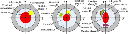
Table 1. Parameters of coronary vessel phantoms.

Tissue name		Composition	Average refractive index	Optical absorption coefficient (cm^−1)	Optical scattering coefficient (cm^−1)	Anisotropy factor	Average SoS (m/s)	Density (kg/L)
Adventitia	1#	Connective tissue	1.41	0.20	20	0.80	1600	1.12
	2#
	3#
Intima/Media	1#	Muscular tissue	1.41	0.20	20	0.80	1570	1.10
	2#
	3#
Lumen	1#	Blood	1.34	0.10	800	0.99	1540	1.00
	2#
	3#
Fibrous cap	1#	Fibrous tissue	1.46	0.01	80	0.75	1610	0.96
	2#
Calcified plaque	1#	Calcium	1.46	0.04	80	0.80	1650	1.36
	2#
Lipid-rich plaque	1#	Lipid	1.46	0.55	500	0.80	1480	0.92
	2#
Fibro-lipid plaque	1#	Fibrous and lipidic tissue	1.46	0.01	20	0.75	1610	0.90
	2#

3.2. Results of forward simulation

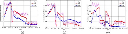
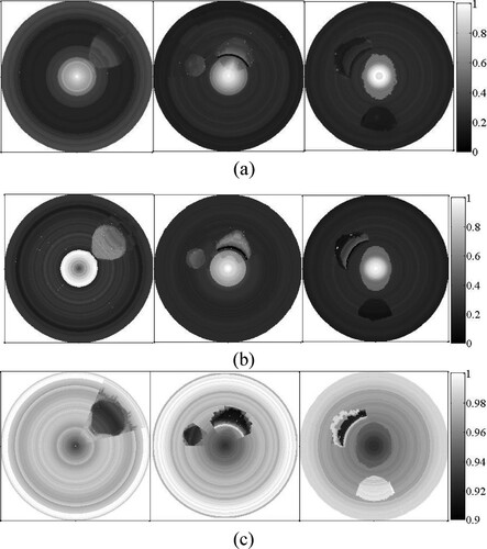
Figure 3 shows the images of AOED and initial acoustic pressure obtained by forward simulation. The images in Figure 3(b) are the distribution images of the PA signals including Gaussian white noise with the signal-to-noise ratio of 60 dB. The optical deposition of the tissues with different components depends on their OACs. The lumen, lipid and fibro-lipid are shown as the brighter regions in Figure 3 because their OACs are larger than other tissues. Figure 4 presents the comparison between the normalized AOED and the OAC at the centre of the plaques, where adjacent peaks or troughs indicate the same tissue composition. The location of the plaques as well as different components in the same plaque can be identified according to these plots. However, the three-layer structures of the vessel wall cannot be distinguished clearly because of the similar optical parameters of the intima, media and adventitia.

Figure 3. Results of forward simulation of vessel phantoms. (a) AOED; (b) Initial pressure.

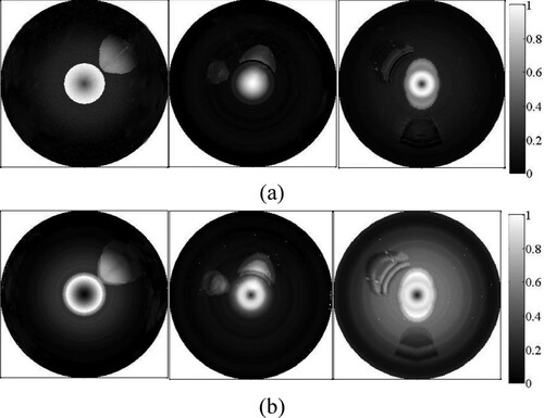
Figure 4. Plots of preset OAC and normalized AOED simulated by using RTE and Monte Carlo (MC) respectively. (a) Vessel phantom a (θ = 41°); (b) Vessel phantom b (θ = 74°); (c) Vessel phantom c (θ = 144°).

3.3. Results of simultaneous recovery of AOED, OAC and SoS distribution

Figure 5 shows the results of the joint reconstruction, where A₀ = 0.05, μ_a,0 = 0.05, c₀ = 1430 m/s, l_A = 0.05, l_μa = 0.05 and l_c = 10 m/s. The plaque contours are clearer in the AOED image than in the SoS image. However, the AOED image can only roughly locate the plaques, while the OAC image can quantitatively depict the location, size, shape and optical properties of the plaques.

Figure 5. Results of image reconstruction. (a) AOED; (b) OAC; (c) SoS.

Figures 6 and 7 provide the comparison between the reconstructed and the preset AOED, OAC and SoS at several measuring locations, which suggests that the reconstructions are very close to the preset values.

Figure 6. Plots of reconstructed and preset normalized AOED, OAC and SoS at several measuring locations. (a) Vessel phantom a; (b) Vessel phantom b; (c) Vessel phantom c.

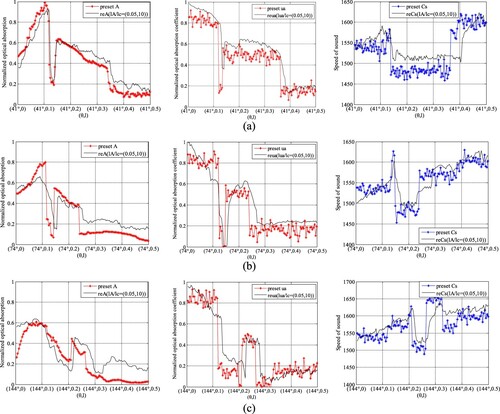
Figure 7. Root mean square (RMS) errors between reconstructed and preset values at several fixed measuring locations. (a) Normalized AOED and OAC; (b) SoS.

4. Discussion

4.1. Influence of iteration step size on reconstruction quality

In this section, the influence of the iteration step sizes, i.e. l_A, l_μa and l_c, on reconstruction quality is discussed based on the experimental results by changing l_A, l_μa and l_c while other parameters remained unchanged. i.e. A₀ = 0.05, μ_a,0 = 0.05 and c₀ = 1430 m/s.

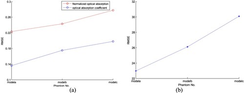
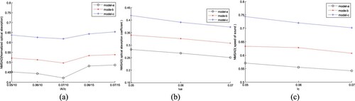
In AOED estimation, (l_A, l_c) was set as (0.06, 10 m/s), (0.07, 10 m/s), (0.06, 15 m/s) and (0.07, 15 m/s) respectively, while in OAC estimation, (l_μa, l_c) was set as (0.05, 10 m/s), (0.06, 10 m/s) and (0.07, 10 m/s) respectively. The reconstruction results are shown in Figures 8 and 9. The normalized mean square absolute distance (NMSAD) between the reconstructions and the preset values listed in Table 1 was adopted to quantitatively evaluate the reconstruction quality. Lower NMSAD indicates higher reconstruction quality. The results shown in Figure 10 indicate that (l_A,l_μa,l_c) = (0.07, 0.07, 10 m/s) leads to the lowest NMSAD. Thus, we took it as the optimal step size in the subsequent experiments.

Figure 8. Reconstructed images of (a) AOED, (b) SoS and (c) OAC in the case of different iteration step sizes. In each subfigure, the top, middle and bottom row present the results of the vessel phantom a, b and c respectively. In each row of subfigure (a) and (b), from left to right, (l_A, l_c) is (0.06, 10 m/s), (0.07, 10 m/s), (0.06, 15 m/s) and (0.07, 15 m/s) respectively. In each row of subfigure (c), from left to right, l_μa is 0.05, 0.06 and 0.07 respectively.

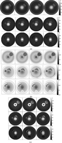
Figure 9. Reconstructed and preset values of (a) normalized AOED and (b) OAC at several measuring locations in the case of different iteration step sizes. In each subfigure, from left to right, the result is obtained for the vessel phantom a, b and c respectively.

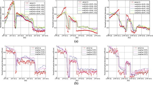
Figure 10. NMSADs of images reconstructed with different iteration step sizes. (a) AOED; (b) OAC; (c) SoS.

4.2. Influence of initial plans of iteration on reconstruction quality

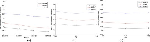
We compared the reconstruction results obtained by changing the initial plans of iteration, i.e. A₀, c₀(r) and μ_a,0, while other parameters remained unchanged, i.e. (l_A, l_μa, l_c) = (0.07, 0.07, 10 m/s). We set (A₀, c₀) as (0.07, 1400 m/s), (0.05, 1430 m/s), (0.07, 1430 m/s) respectively in AOED estimation, while (μ_a,0, c₀) as (0.05, 1430 m/s), (0.07, 1430 m/s) and (0.09, 1430 m/s) respectively in OAC estimation. The results shown in Figures 11 and 12 suggest that (A₀, μ_a,0, c₀) = (0.07, 0.07, 1430 m/s) leads to the lowest NMSAD of the reconstructed images.

Figure 11. Reconstructed and preset values of (a) normalized AOED and (b) OAC at some measuring locations in the case of different initial plans of iteration. In each subfigure, from left to right, the result is obtained for the vessel phantom a, b and c respectively.

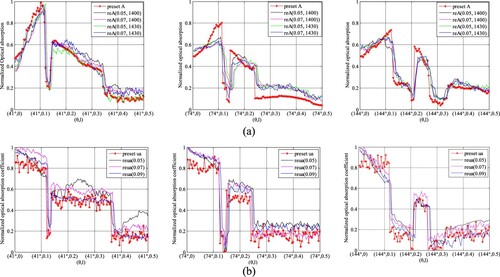
Figure 12. NMSADs of reconstructed images in the case of different initial plans of iteration. (a) Normalized AOED; (b) OAC; (c) SoS.

4.3. Compare with reconstructions based on a fixed SoS

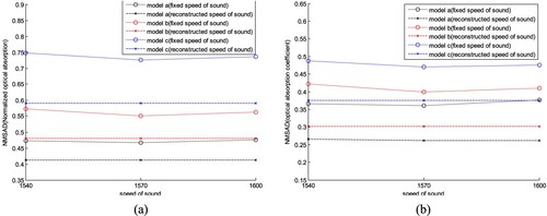
We compared the reconstructions provided by the proposed method with those obtained by using a fixed SoS. According to the discussions in Sections 4.1 and 4.2, we set (A₀, μ_a,0, c₀) = (0.07, 0.07, 1430 m/s) and (l_A, l_μa, l_c) = (0.07, 0.07, 10 m/s). Then, we reconstructed the images of the AOED and OAC with a fixed SoS of 1540, 1570 and 1600 m/s respectively. The results are shown in Figures 13 and 14, where the horizontal line in Figure 14 represents the NMSAD of the image reconstructed by use of the proposed method in this work. Obviously, the proposed method can provide the reconstructions with higher quality than the fixed SoS reconstructions.

Figure 13. Images obtained with the proposed method and the fixed SoS method. In each subfigure, the top, middle and bottom row present the results of the vessel phantom a, b and c respectively. In each row, from left to right, the image is obtained by using the proposed method, fixed SoS of 1540, 1570, and 1600 m/s respectively. (a) AOED; (b) OAC.

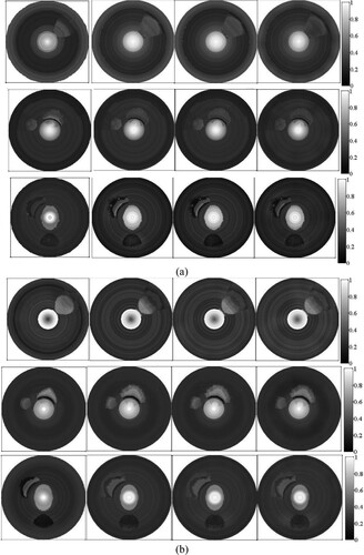
Figure 14. NMSAD of images obtained with the proposed method and the fixed SoS method. (a) AOED; (b) OAC.

4.4. Compare with delay compensation method

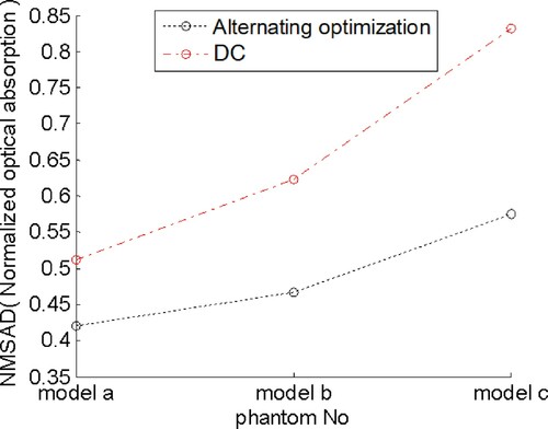
In this section, we compared the results of AOED reconstruction obtained by use of the method in this work and the delay compensation (DC) method in [17] which is a study dedicated to endoscopic PAT. The DC method compensates for the deviation in the ultrasonic propagation time caused by the variable SoS by determining an optimal SoS providing the maximal local focusing at each measuring location. The results shown in Figures 15 and 16 suggest that the method in this work outperforms the DC method in the visualization and the NMSAD of the reconstructed images.

Figure 15. AOED images of three vessel phantoms obtained with the proposed method and the DC method.

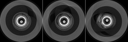
Figure 16. NMSAD of images obtained with the the proposed method and the DC method.

4.5. Compare with two-step qIVPAT algorithm

In this section, we compared the results of OAC estimation by use of the proposed method with those provided by a two-step algorithm published in our previous work [4]. The two steps are as follows. First, the AOED is reconstructed from the acoustic measurements by using a conventional reconstruction method such as filtered back-projection (FBP) or TR. 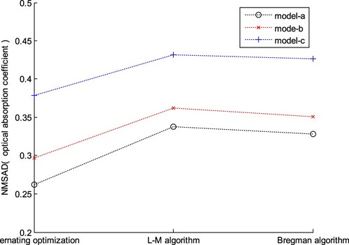Second, the OAC is estimated through solving a NLS problem as follows, (40) ${\hat{\mu }}_{\text{a}}(\mathbf{\text{r}})=\underset{{\mu }_{\text{a}}\ge 0}{\arg min}[\Vert A_{\text{m}}(\mathbf{\text{r}})-C\cdot A(\mathbf{\text{r}},{\mu }_{\text{a}}(\mathbf{\text{r}})){\Vert }^2+\gamma \Vert {\mu }_{\text{a}}(\mathbf{\text{r}}){\Vert }_{\text{TV}}],$(40) where A_m(r) is the measured (i.e. reconstructed) AOED at r, C is the calibration factor related to the signal acquisition system, A(r, μ_a(r)) is the theoretical AOED regarding the OAC which is obtained by forward simulation, and γ is the regularization parameter. In the comparison experiments, we took the AOED reconstructed by using the method in Section 2.2 as A_m(r), where (A₀, c₀) = (0.07, 1430 m/s) and (l_A, l_c) = (0.07, 10 m/s). Then, we utilized the L-M algorithm and Bregman algorithm [34] to solve eq.(40) respectively. The results are shown in Figures 17 and 18. Obviously, the NMSADs of the two-step algorithm are higher than those of the method in this study, indicating lower reconstruction quality.

Figure 17. OAC images provided by the two-step algorithm. (a) L-M optimization; (b) Bregman optimization.

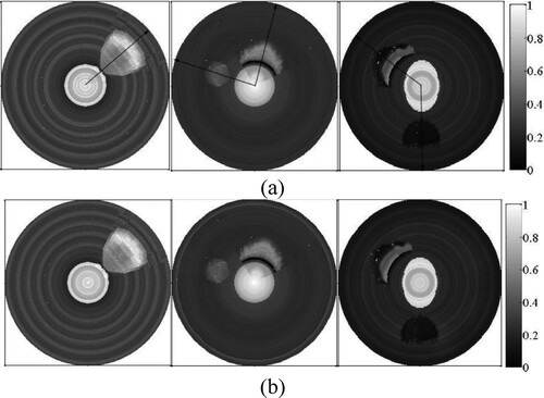
Figure 18. NMSADs of OAC images provided by the method in this work and the two-step algorithm.

In order to quantitatively evaluate the accuracy of the OAC estimation, we measured the radial thickness of a plaque along the arrow in each image shown in Figure 17(a) and compared it with the true value listed in Table 1. The results listed in Table 2 demonstrate that the measured thickness of a plaque with single component is basically consistent with the true value, whereas that of a mixed plaque with multiple components has relatively larger error. Moreover, the measured thickness of the reconstructions by use of the proposed method is more accurate than that by the two-step algorithm.

Table 2. True and measured thickness of the plaques.

		Plaque thickness (cm)
			Measured
Vessel phantom	Plaque	True	Proposed method	Two-step method (L-M)	Two-step method (Bregman)
a	Lipid-rich plaque 1#	0.227	0.233	0.249	0.247
b	Lipid-rich plaque 2#	0.121	0.133	0.146	0.141
	Fibro-lipid plaque 1#	0.104	0.121	0.142	0.133
c	Calcified plaque 1# Fibro-lipid plaque 2#	0.129	0.139	0.158	0.154
	Calcified plaque 2#	0.146	0.158	0.167	0.160

5. Conclusion

The novelty of this work is to present an approach to improve image quality of IVPAT in tissues with the variable SoS by simultaneously reconstructing images of the AOED, OAC and SoS distribution in the vascular cross-sections from the measured acoustic pressure. We minimized the error functions between the measured and the theoretical acoustic pressure regarding AOED, OAC and SoS which was obtained by forward numerical simulation to achieve the joint reconstruction. We solved the NLS problems in the way of alternating iterative optimization. Demonstration results indicate that this approach can implement the quantitative description of both the acoustic and optical properties of tissues in the vascular cross-sections. The AOED images display the morphological structures and the SoS and the OAC images present the quantitative information regarding the acoustic and optical properties. Discussions indicate that the reconstruction accuracy is influenced by the initial plan and iteration step size which should be properly set to obtain satisfactory reconstruction quality. Comparison results suggest that the AOED images provided by the proposed approach are closer to the simulations than those obtained with a fixed SoS and the DC method. In addition, compared with the two-step algorithm of estimating the OAC, this approach can not only avoid the possible errors in reconstructing the optical absorption, but also reduce the image quality degradation caused by the ideal premise of the fixed SoS.

In this preliminary study, we ignored the continuous variations in the optical and acoustic parameters of tissues illuminated by short laser pulses due to the changes in temperature and thermal damage. We will take into account the influence of the photothermal conversion and the temperature on the characteristic parameters of tissues in the future work. In addition, photoacoustically generated ultrasound is usually reflected, scattered and refracted when propagating in biological tissues with different thickness, density and acoustic properties leading to acoustic attenuation. In this work, we only considered the influence of the heterogeneously distributed SoS on the image reconstruction while ignored acoustic attenuation.

It is a large-scale, nonlinear, unstable, and ill-conditioned inverse problem to simultaneously reconstruct the optical absorption property and SoS distribution in each vascular cross-section from intravascular PA measurements. The reconstruction accuracy is inevitably reduced by the errors in the NLS model. Further optimization of the model is needed to improve the stability of the results. Furthermore, as a full-wave inversion scheme, efficient optimization tools being used to reduce the computational burden are one of key problems to be solved in the future work.

Although the PA image quality can be improved by simultaneously recovering AOED/OAC and SoS, it is actually a difficult task to accurately reconstruct the SoS distribution from only the PA measurement even if the complete data is collected. A more precise method is to combine the PA measurement with other measurements such as ultrasonic scanning. The combined PAUS imaging [35] acquires time series of PA pressure and ultrasonic echoes reflected by the target with a single imaging system at the same time. It will be a major trend in the future to utilize an intravascular two-modal PAUS technique [36] implementing simultaneous imaging of the SoS and the optical absorption property.

Acknowledgments

This work was supported by National Nature Science Foundations of China (no. 62071181).

Disclosure statement

No potential conflict of interest was reported by the author(s).

Additional information

Funding

This work was supported by National Nature Science Foundations of China [grant number 62071181].

Appendix. Derivation of the iterative increment of SoS in estimating OAC

The optimization problem of the SoS estimation in simultaneous reconstruction of OAC and SoS is as follows, (A1) $\hat{c}(\mathbf{\text{r}})=\underset{c\ge 0}{\arg min}((1-\beta )\Vert p_{\text{e}}(\mathbf{\text{r}},{\mu }_{\text{a}}(\mathbf{\text{r}}),c(\mathbf{\text{r}}))-p_{\text{m}}(\mathbf{\text{r}}){\Vert }^2+\beta \Vert c(\mathbf{\text{r}})-c_0(\mathbf{\text{r}}){\Vert }^2),$(A1) which is written equivalently as (A2) $\hat{c}(\mathbf{\text{r}})=\underset{c\ge 0}{\arg min}{\Vert \left(\begin{array}{c}\sqrt{1-\beta }[p_{\text{e}}(\mathbf{\text{r}},{\mu }_{\text{a}}(\mathbf{\text{r}}),c(\mathbf{\text{r}}))-p_{\text{m}}(\mathbf{\text{r}})]\\ \sqrt{\beta }[c(\mathbf{\text{r}})-c_0(\mathbf{\text{r}})]\end{array}\right)\Vert }^2.$(A2)

For convenience, we take (A3) $g(c(\mathbf{\text{r}}))=\Vert p_{\text{e}}(\mathbf{\text{r}},{\mu }_{\text{a}}(\mathbf{\text{r}}),c(\mathbf{\text{r}}))-p_{\text{m}}(\mathbf{\text{r}}){\Vert }^2.$(A3) p_e(r,µ_a(r),c(r)) and c(r)–c₀(r) in eq.(A.2) are linearized at c_k(r) and the high-order terms are ignored obtaining, (A4) $\arg min{\Vert \left(\begin{array}{c}\sqrt{1-\beta }[\mathbf{\text{B}}(c_k(\mathbf{\text{r}}))d\text{(}{c}_k(\mathbf{\text{r}}))+(p_{\text{e}}(\mathbf{\text{r}},{\mu }_{\text{a,}k}(\mathbf{\text{r}}),c_k(\mathbf{\text{r}}))-p_{\text{m}}(\mathbf{\text{r}}))]\\ \sqrt{\beta }[\mathbf{\text{I}}d\text{(}{c}_k(\mathbf{\text{r}}))+c_k(\mathbf{\text{r}})-c_0(\mathbf{\text{r}})]\end{array}\right)\Vert }^2,$(A4) where c_k(r) and μ_a,k(r) are the SoS and OAC respectively in the k-th iteration, d(c_k(r)) is the iterative increment of c_k(r), B(c_k(r)) is the Jacobian matrix of g(c_k(r)), and I is the unit matrix. According to the principle of nonlinear least squares, we obtain (A5) $\begin{array}{rl}& {\Vert \left(\begin{array}{c}\sqrt{1-\beta }[\mathbf{\text{B}}(c_k(\mathbf{\text{r}}))d\text{(}{c}_k(\mathbf{\text{r}}))+(p_{\text{e}}(\mathbf{\text{r}},{\mu }_{\text{a,}k}(\mathbf{\text{r}}),c_k(\mathbf{\text{r}}))-p_{\text{m}}(\mathbf{\text{r}}))]\\ \sqrt{\beta }[\mathbf{\text{I}}d\text{(}{c}_k(\mathbf{\text{r}}))+c_k(\mathbf{\text{r}})-c_0(\mathbf{\text{r}})]\end{array}\right)\Vert }^2\\ & ={\left[\begin{array}{c}\sqrt{1-\beta }[\mathbf{\text{B}}(c_k(\mathbf{\text{r}}))d\text{(}{c}_k(\mathbf{\text{r}}))+(p_{\text{e}}(\mathbf{\text{r}},{\mu }_{\text{a,}k}(\mathbf{\text{r}}),c_k(\mathbf{\text{r}}))-p_{\text{m}}(\mathbf{\text{r}}))]\\ \sqrt{\beta }[\mathbf{\text{I}}d\text{(}{c}_k(\mathbf{\text{r}}))+c_k(\mathbf{\text{r}})-c_0(\mathbf{\text{r}})]\end{array}\right]}^T\\ & \left[\begin{array}{c}\sqrt{1-\beta }[\mathbf{\text{B}}(c_k(\mathbf{\text{r}}))d\text{(}{c}_k(\mathbf{\text{r}}))+(p_{\text{e}}(\mathbf{\text{r}},{\mu }_{\text{a,}k}(\mathbf{\text{r}}),c_k(\mathbf{\text{r}}))-p_{\text{m}}(\mathbf{\text{r}}))]\\ \sqrt{\beta }[\mathbf{\text{I}}d\text{(}{c}_k(\mathbf{\text{r}}))+c_k(\mathbf{\text{r}})-c_0(\mathbf{\text{r}})]\end{array}\right]\end{array}$(A5)

By further deriving from Equation (A5), we obtain (A6) $\begin{array}{rl}& \text{2}{\left[\begin{array}{c}\sqrt{1-\beta }\mathit{B}(c_k(\mathbf{\text{r}}))\\ \sqrt{\beta }\mathbf{\text{I}}\end{array}\right]}^T\left[\begin{array}{c}\sqrt{1-\beta }\mathit{B}(c_k(\mathbf{\text{r}}))\\ \sqrt{\beta }\mathbf{\text{I}}\end{array}\right]d\text{(}{c}_k(\mathbf{\text{r}}))\\ & +2\left[\begin{array}{c}\sqrt{1-\beta }\mathbf{\text{B}}(c_k(\mathbf{\text{r}}))\\ \sqrt{\beta }\mathbf{\text{I}}\end{array}\right]\left[\begin{array}{c}\sqrt{1-\beta }[p_{\text{e}}(\mathbf{\text{r}},{\mu }_{\text{a,}k}(\mathbf{\text{r}}),c_k(\mathbf{\text{r}}))-p_{\text{m}}(\mathbf{\text{r}})]\\ \sqrt{\beta }[c_k(\mathbf{\text{r}})-c_0(\mathbf{\text{r}})]\end{array}\right]=0\end{array}$(A6)

Simple algebra shows that (A7) $\begin{array}{rl}d\text{(}{c}_k(\mathbf{\text{r}}))& ={\left[\begin{array}{c}(1-\beta ){[(1-\beta ){\mathbf{\text{B}}}^T(c_k(\mathbf{\text{r}}))\mathbf{\text{B}}(c_k(\mathbf{\text{r}}))+\beta \mathbf{\text{I}}]}^{-1}{\mathbf{\text{B}}}^T(c_k(\mathbf{\text{r}}))\\ \beta {[(1-\beta ){\mathbf{\text{B}}}^T(c_k(\mathbf{\text{r}}))\mathbf{\text{B}}(c_k(\mathbf{\text{r}}))+\beta \mathbf{\text{I}}]}^{-1}\end{array}\right]}^T\\ & \times \left[\begin{array}{c}{p}_{\text{e}}(\mathbf{\text{r}},{\mu }_{\text{a,}k}(\mathbf{\text{r}}),c_k(\mathbf{\text{r}}))-p_{\text{m}}(\mathbf{\text{r}})\\ c_k(\mathbf{\text{r}})-c_0(\mathbf{\text{r}})\end{array}\right]\end{array}$(A7)

References

- Cao Y, Kole A, Hui J, et al. Fast assessment of lipid content in arteries in vivo by intravascular photoacoustic tomography. Sci Rep. 2018;8(1):2400.
- Jansen K, Soest GV, Van de Steen AFW. Intravascular photoacoustic imaging: a new tool for vulnerable plaque identification. Ultrasound Med Biol. 2014;40(6):1037–1048.
- Sun Z, Han D, Yuan Y. 2-D image reconstruction of photoacoustic endoscopic imaging based on time-reversal. Comput Biol Med. 2016;76:60–68.
- Sun Z, Zheng L. Reconstruction of optical absorption coefficient distribution in intravascular photoacoustic imaging. Comput Biol Med. 2018;97:37–49.
- Yao J, Wang LV. Recent progress in photoacoustic molecular imaging. Curr Opin Chem Biol. 2018;45:104.
- Poudel J, Yang L, Anastasio MA. A survey of computational frameworks for solving the acoustic inverse problem in three-dimensional photoacoustic computed tomography. Physics in Medicine & Biology. 2019;64, 14TR01. https://iopscience.iop.org/article/https://doi.org/10.1088/1361-6560/ab2017.
- Xia J, Huang C, Maslov K, et al. Enhancement of photoacoustic tomography by ultrasonic computed tomography based on optical excitation of elements of a full-ring transducer array. Opt Lett. 2013;38(16):3140–3149.
- Jin X, Wang LV. Thermoacoustic tomography with correction for acoustic speed variations. Phys Med Biol. 2006;51(24):6437–6448.
- Palamodov V. Time reversal in photoacoustic tomography and levitation in a cavity. Inverse Probl. 2014;30(12):125006.
- Qian J, Stefanov P, Uhlmann G, et al. An efficient Neumann series–based algorithm for thermoacoustic and photoacoustic tomography with variable sound speed. SIAM J Imaging Sci. 2011;4(4):850–883.
- Haltmeier M, Nguyen LV. Iterative methods for photoacoustic tomography with variable sound speed. SIAM J Imaging Sci. 2016;10(2):751–781.
- Huang C, Wang K, Nie L, et al. Full-wave iterative image reconstruction in photoacoustic tomography with acoustically inhomogeneous media. IEEE Trans Med Imaging. 2013;32(6):1097–1110.
- Zhang C, Wang Y. A reconstruction algorithm for thermoacoustic tomography with compensation for acoustic speed heterogeneity. Phys Med Biol. 2008;53(18):4971–4982.
- Treeby BE, Varslot TK, Zhang EZ, et al. Automatic sound speed selection in photoacoustic image reconstruction using an autofocus approach. J Biomed Opt. 2011;16(9):090501.
- Cong B, Kondo K, Namita T, et al. Photoacoustic image quality enhancement by estimating mean sound speed based on optimum focusing. Jpn J Appl Phys. 2015;54(7S1). 07HC13. https://iopscience.iop.org/article/https://doi.org/10.7567/JJAP.54.07HC13.
- Ye M, Cao M, Feng T, et al. Automatic speed of sound correction with photoacoustic image reconstruction. Proceedings of SPIE International Conference on Photons Plus Ultrasound: Imaging and Sensing. 15 Mar. 2016, 9708: 97083D.
- Sun Z, Jia Y. An image reconstruction method for endoscopic photoacoustic tomography in tissues with heterogeneous sound speed. Comput Biol Med. 2019;110:15–28.
- Xia J, Huang C, Maslov K, et al. Enhancement of photoacoustic tomography by ultrasonic computed tomography based on optical excitation of elements of a full-ring transducer array. Virtual Journal for Biomedical Optics. 2013;8(9):3140–3143.
- Yuan Z, Zhang Q, Jiang H. Simultaneous reconstruction of acoustic and optical properties of heterogeneous media by quantitative photoacoustic tomography. Opt Express. 2006;14(15):6749–6754.
- Jiang H, Yuan Z, Gu X. Spatially varying optical and acoustic property reconstruction using finite element-based photoacoustic tomography. J Opt Soc Am A Opt Image Sci Vis. 2006;23(4):878–888.
- Zhang J, Wang K, Yang Y, et al. Simultaneous reconstruction of speed-of-sound and optical absorption properties in photoacoustic tomography via a time-domain iterative algorithm. Proceedings of SPIE International Conference on Photons Plus Ultrasound: Imaging and Sensing 2008, 28 Feb. 2008, 6856: 68561F.
- Huang C, Wang K, Schoonover RW, et al. Simultaneous reconstruction of absorbed optical energy density and speed of sound distributions in photoacoustic computed tomography. Proceedings of SPIE International Conference on Photons Plus Ultrasound: Imaging and Sensing 2014, 19 Feb. 2014, 8943: 894360.
- Huang C. Image reconstruction in photoacoustic computed tomography with acoustically heterogeneous media. Ph.D. Dissertation, Washington University, 2014.
- Huang C, Wang K, Schoonover RW, et al. Joint reconstruction of absorbed optical energy density and sound speed distributions in photoacoustic computed tomography: a numerical investigation. IEEE Trans Comput Imaging. 2016;2(2):136–149.
- Sheu YL, Chou CY, Hsieh BY. Image reconstruction in intravascular photoacoustic imaging. IEEE Transactions on Ultrasonics Ferroelectrics and Frequency Control. 2011;58(10):2067–2077.
- Sun Z, Yuan Y, Han D. A computer-based simulator for intravascular photoacoustic images. Comput Biol Med. 2017;81:176–187.
- Gao H, Osher S, Zhao H. Mathematical Modeling in Biomedical imaging II. Berlin/Heidelberg: Springer; 2012. p. 131–158.
- Cox BT, Laufer JG, Arridge SR, et al. Quantitative spectroscopic photoacoustic imaging: a review. J Biomed Opt. 2012;17(6):061202.
- Treeby BE, Zhang EZ, Cox BT. Photoacoustic tomography in absorbing acoustic media using time reversal. Inverse Probl. 2010;26(11):115003.
- Tang YC, Wu GR, Zhu CX. An inner-outer iteration method for solving convex optimization problems involving the sum of three convex functions. Scientia Sinica Mathematica. 2019;49(5):831–858.
- Zheng E. Several regularization methods for ill-posed problems and their numerical realization. Master Thesis. Jilin University, 2009.
- Amir B, Teboulle M. A fast iterative shrinkage-thresholding algorithm for linear inverse problems. SIAM J Imaging Sci. 2009;2(1):183–202.
- Jacques SL. Optical properties of biological tissues: a review. Phys Med Biol. 2013;58(11):R37–R61.
- Kuchment P. The mathematical legacy of Leon Ehrenpreis. Milan: Springer; 2012. p. 183.
- Matthews TP, Anastasio MA. Joint reconstruction of the initial pressure and speed of sound distributions from combined photoacoustic and ultrasound tomography measurements. Inverse Probl. 2017;33(12):124002.
- Li Y, Chen Z. Multimodal intravascular photoacoustic and ultrasound imaging. Biomed Eng Lett. 2018;8:193–201.