Inverse scattering problem for detecting a defect in a magnetoelastic layer

ABSTRACT

This work is devoted to studying a direct and inverse scattering problem for a magnetoelastic layer having a defect, in the frame of the electromagnetic theory. In terms of the displacement field over the defect's contour, a coupled system of boundary integral equations is formulated, for magnetically permeable and impermeable defects. To identify the position and size of the defect, an efficient numerical algorithm is developed by using the quasi-Newton iterative method. In order to check the influence of the magnetic field upon the scattering waves from the layer, a series of numerical examples is presented with different noise levels. The results showed that the magnetic field has a sensitive effect on the identification process when the external magnetic field increases, especially for the materials having a high magnetic permeability factor ${\mu }_r$. Also, a special inverse problem for predicting the external applied magnetic field, upon a copper layer having a defect with various sizes, has been performed.

Keywords:

• Magnetoelasticity
• inverse scattering problem
• time-Harmonic load
• Green's functions
• boundary integral equations

2010 Mathematics Subject Classifications:

• Partial differential equations
• Integral equations
• Mechanics of deformable solids
• Numerical analysis
• Calculus of variations and optimalcontrol
• optimization

1. Introduction

During recent years, a large number of theoretical and experimental works is devoted to studying the response of deformable solids subjected to electromagnetic fields, owing to their extensive applications in various branches of science as Geophysics, Acoustics, health monitoring systems and Astrophysics. Recently, this topic has received new impetus due to the development in the so-called smart materials, which have one or more properties significantly controlled by any external fields such as; temperature, moisture, pH, and electric or magnetic fields.

The problems of mechanical wave propagation in the presence of a magnetic field have been investigated by many researchers. The first study was done by Knopoff [1], who investigated the propagation of seismic waves in the presence of Earth's magnetic field. Dunkin and Eringen [2] studied the effect of high magnetostatic and electrostatic fields on plane waves traveling through an infinite plate under the assumption that the resulting electromagnetic fields are quasistationary. The problem of coupled electromagnetic and elastic waves, for both linear and nonlinear interaction such as magnon-phonon coupling and magneto-acoustic resonance, is reviewed by Maugin [3]. Some studies were devoted to investigating the wave propagation in various media under a magnetic field by Das and Bhattacharya [4], Gourakishwar [5], Andreou and Dassios [6], especially when the medium is of isotropic homogeneous materials. The basic equations of electromagnetic interactions in elastic solids and general details about various mechanical problems coupled with electromagnetic fields are displayed in the articles [7–9]. While other papers are concerned with analyzing the propagation of surface waves under the effect of a primary magnetic field [10–13]. The studies are carried out on electrically conducting elastic solid, and the frequencies equations have been derived. Moreover, the relation between Rayleigh wave velocity and the strength of the primary magnetic field is investigated.

Recently, in fracture mechanics, the problem of a crack in an elastic material under electromagnetic-mechanical loading has attracted more attention. The problem of cracks lying on the interface of two dissimilar ferromagnetic materials subjected to a uniform magnetic field is discussed by Lin and Lin [14]. Rogowski [15] investigated the effects of magnetic boundary conditions (limited permeability) on the crack surface in piezomagnetic materials under magneto-mechanical loading. Bagdasarian and Hasanian [16] developed a numerical method to determine the displacements and the magnetoelastic stress intensity factor of a crack-opening for various boundary conditions. According to the linear model of magnetoelasticity, Wei et al. [17], Lin and Yeh [18], and Hasebe et al. [19] discussed the effect of a strong magnetic field upon a finite plane crack in soft ferromagnetic materials by using the complex potential theory.

On the other hand, some theoretical papers were devoted to scattering and inverse scattering problems by cracks or defects in magneto-electro-elastic (MEE) materials based on the boundary integral equations (BIE) technique. Nowacki [20], Sladek and Sladek [21] derived the general boundary integral equations for various boundary value problems in magnetoelasticity and thermoelasticity by using the reciprocity theorem and Green's function. Fang [22,23] investigated the multiple scattering electroelastic waves from an object in a piezoelectric medium analytically. Jinxi et al. [24] derived 2D-Green's functions for anisotropic MEE materials, with a cavity in an elliptic form, under mechanical loading by using a conformal mapping technique. However, Qin [25] obtained 2D-Green's functions for MEE materials under thermal loading in a closed-form. All aforementioned works can be considered direct scattering problems by cracks in those materials.

Moreover, some other theoretical papers are concerned with the inverse problems in MEE materials. Lorenzi and Priimenko [26] discussed the existence and uniqueness of the solutions, while Priimenko and Vishnevskii [27,28] developed explicit analytical forms and numerical algorithms to identify the problem's parameters. Avdeev et al. [29] and Romanov [30] demonstrated the stability of the reconstruction algorithm for the material parameters for a layered medium in the context of a coupled linearized set of electro-magneto-elasticity equations. The artificial neural network technique is applied by Lu et al. [31] to analyze the identification of crack damage in Aluminium effectively. This method was used again by Hattori and Saez [32] to improve the process of identification in MEE materials, even for high levels of noise.

However, the applications of the boundary integral equations are limited to solving the scattering and inverse scattering problems due to several difficulties arising in the determination of Green's functions and regularization singularities of these integrals. We succeed, to present some papers analyzing the scattering and inverse scattering problems in elastodynamics by a time-harmonic load applied upon medium involving objects or cracks, based on the boundary integral equations method [33–36].

The aim of current work is to analyze the influence of a quasi-static electromagnetic field on the process of detecting a defect in an elastic layer. The latter subjected to a time-harmonic load, with fixed circular frequency, applied to its upper boundary surface. In the first section, Maxwell's equations reviewed as a result of the interaction of a primary magnetic field with an isotropic elastic medium.

We formulated a direct and inverse scattering problem in the context of the electromagnetic theory by an elliptic defect or cavity in a homogeneous isotropic elastic layer subjected to a constant external magnetic field but the defect is free of any stresses. The problem is investigated for a two-dimension dynamic strain in-plane problem of a single magnetoelastic layer subjected to a time-harmonic load upon the upper layer boundary. By using the reciprocity theorem, a system of coupled boundary integral equations (BIEs) is obtained over the defect's contour, for both cases if the defect is magnetically permeable or impermeable. The fundamental solutions, or the Green's strain functions and stresses, are constructed for a conductive magnetoelastic layer subjected to homogeneous boundary conditions. By using the boundary element method the basic boundary integral equations system is solved numerically. As a result, the solution of the direct problem allows finding the scattered surface field on the upper surface of the layer. This surface field has been used as input data, with levels of noise, to formulate the respective identification inverse problem of the defects. A numerical algorithm to defect identification in different materials is developed by reducing the inverse problem into an unconstrained optimization problem. A series of numerical examples, on the detection algorithm in the case of exact and noisy data, is performed. On the other hand, special examples of the prediction of the external applied magnetic field on a conductive layer, containing, defects are presented.

2. Basic equations

Let us consider a perfectly isotropic and homogeneous elastic layer, subjected to a constant magnetic field $\mathit{B}$ inducing an electric field $\mathit{E}$ in the medium. The electric field is normal to the magnetic intensity and the displacement vector $\mathit{u}$. The governing equation of the linear interaction of the electromagnetic field with the mechanical loading is given by [2]: (1) $\mathrm{\nabla }\cdot \sigma +\mathit{J}\times \mathit{B}+\mathit{X}=\rho \ddot{\mathit{u}},$(1) where $\sigma$ denotes for the Cauchy stress tensor, $\mathit{X}$ is the elastic body force, $\mathit{u}$, ρ are the mechanical displacement vector, and mass density, respectively. The term $\mathit{J}\times \mathit{B}$ refers to the Lorentz force exerted on a unit volume element of a current density $\mathit{J}$ in a magnetic induction field $\mathit{B}$.

According to Nowacki, when the frequencies of the mechanical waves are much smaller than those of electromagnetic waves but have the same wavelength, then the electromagnetic field may be regarded as quasistatic [20]. Mathematically it means $\mathit{D}=0,\mathrm{\partial }\mathit{D}/\mathrm{\partial }t=0$. Therefore, Maxwell's equations will be: (2) $\mathrm{\nabla }\times \mathit{E}=-\frac{\mathrm{\partial }\mathit{B}}{\mathrm{\partial }t},\mathrm{\nabla }\cdot \mathit{B}=0,\mathrm{\nabla }\times \mathit{H}=\mathit{J},$(2) where $\mathit{H}$ is the magnetic field, and the free charges in the medium are absent. The electric current is given by: (3) $\mathit{J}={\sigma }_0\left[\mathit{E}+\left(\frac{\mathrm{\partial }\mathit{u}}{\mathrm{\partial }t}\times \mathit{B}\right)\right],\mathit{B}=\mu \mathit{H},$(3) where ${\sigma }_0$, μ are the electric conductivity and permeability of the medium, respectively. Take into account the constitutive elastic equation is given by (4) ${\sigma }_{ij}=2G{ϵ}_{ij}+\lambda {\delta }_{ij}{ϵ}_{kk},i,j,k=1,2,3,$(4) where ${ϵ}_{ij}=(u_{i,j}+u_{j,i})/2$ is the elastic strain tensor, G, and λ are Lame's constants for linear isotropic elastic material, and ${\delta }_{ij}$ is the identity tensor.

In the light of the coupling between the electromagnetic field and strain field, there appear small perturbations $\mathit{h}$, and $\mathit{e}$ described by the relations: (5) $\mathit{H}={\mathit{H}}_0+\mathit{h},\mathit{E}=\mathit{e},\mathit{J}=\mathit{j}.$(5) The products of these quantities are small and can be neglected. Therefore Maxwell's and the constitutive equations represent as follows (6) $\begin{array}{rl}\mathrm{\nabla }\times \mathit{e}& =-\mu \frac{\mathrm{\partial }\mathit{h}}{\mathrm{\partial }t},\mathrm{\nabla }\cdot \mathit{h}=0,\mathrm{\nabla }\times \mathit{h}=\mathit{j},\end{array}$(6) (7) $\begin{array}{rl}\mathit{j}& ={\sigma }_0\left(\mathit{e}+\mu \frac{\mathrm{\partial }\mathit{u}}{\mathrm{\partial }t}\times {\mathit{H}}_0\right),\mathit{B}=\mu ({\mathit{H}}_0+\mathit{h}).\end{array}$(7) By inserting the above approximations with $(\mathit{e}=0)$, Equation (1(1) $\mathrm{\nabla }\cdot \sigma +\mathit{J}\times \mathit{B}+\mathit{X}=\rho \ddot{\mathit{u}},$(1) ) takes the form (8) $\mathrm{\nabla }\cdot \sigma -\mu {\mathit{H}}_0\times (\mathrm{\nabla }\times \mathit{h})+\mathit{X}=\rho \ddot{\mathit{u}}.$(8) According to the definition of Maxwell's stress tensor for the quasistatic electromagnetic field, (9) ${\tau }_{ij}=\mu [h_i{H}_{0j}+h_j{H}_{0i}-{\delta }_{ij}{h}_k{H}_{0k}],i,j,k=1,2,3$(9) Consequently, Equation (8(8) $\mathrm{\nabla }\cdot \sigma -\mu {\mathit{H}}_0\times (\mathrm{\nabla }\times \mathit{h})+\mathit{X}=\rho \ddot{\mathit{u}}.$(8) ) can be written as (10) $({\sigma }_{ij}+{\tau }_{ij}{)}_{,j}+X_i=\rho {\ddot{u}}_i,i,j=1,2,3.$(10) Combining Equations (6(6) $\begin{array}{rl}\mathrm{\nabla }\times \mathit{e}& =-\mu \frac{\mathrm{\partial }\mathit{h}}{\mathrm{\partial }t},\mathrm{\nabla }\cdot \mathit{h}=0,\mathrm{\nabla }\times \mathit{h}=\mathit{j},\end{array}$(6) )and (7(7) $\begin{array}{rl}\mathit{j}& ={\sigma }_0\left(\mathit{e}+\mu \frac{\mathrm{\partial }\mathit{u}}{\mathrm{\partial }t}\times {\mathit{H}}_0\right),\mathit{B}=\mu ({\mathit{H}}_0+\mathit{h}).\end{array}$(7) ) and eliminating $\mathit{e}$, yield the differential equation: (11) ${\mathrm{\nabla }}^2\mathit{h}-\text{β}\frac{\mathrm{\partial }\mathit{h}}{\mathrm{\partial }t}+\text{β}\mathrm{\nabla }\times \left(\frac{\mathrm{\partial }\mathit{u}}{\mathrm{\partial }t}\times {\mathit{H}}_0\right)=0,\text{β}=\mu {\sigma }_0.$(11) The formulation has supplemented by considering another set of the governing equations for vacuum, (12) $\begin{array}{l}\mathrm{\nabla }\times {\mathit{E}}^0=-{\mu }_0\frac{\mathrm{\partial }{\mathit{h}}^0}{\mathrm{\partial }t},\mathrm{\nabla }\cdot {\mathit{h}}^0=0,\\ \mathrm{\nabla }\times {\mathit{h}}^0={ϵ}_0\frac{\mathrm{\partial }{\mathit{E}}^0}{\mathrm{\partial }t},\mathrm{\nabla }\cdot {\mathit{E}}^0=0,\end{array}$(12) hence (13) $\left({\mathrm{\nabla }}^2-\frac{1}{c^2}\frac{{\mathrm{\partial }}^2}{\mathrm{\partial }{t}^2}\right){\mathit{h}}^0=0,\left({\mathrm{\nabla }}^2-\frac{1}{c^2}\frac{{\mathrm{\partial }}^2}{\mathrm{\partial }{t}^2}\right){\mathit{E}}^0=0.$(13) Inside and outside the medium, the electromagnetic fields should satisfy the following conditions on the boundary (14) $(\mathit{B}-{\mathit{B}}^0)\cdot \mathit{n}=0,(\mathit{E}-{\mathit{E}}^0)\cdot \mathit{t}=0,(\mathit{H}-{\mathit{H}}^0)\cdot \mathit{t}=0,$(14) where ${\mathit{B}}^0={\mu }_0{\mathit{H}}^0,{\mathit{H}}^0={\mathit{H}}_0+h^0$, $\mathit{t}$ is a unit tangent vector, and $\mathit{n}$ is the outward unit normal vector to the boundary.

2.1. The reciprocity equation

The reciprocal theorem is often used to extract information concerning solutions to a boundary value problem without the need to solve the problem in detail. It is the basis for a computational method in linear elasticity called the boundary element method, which can provide a way to compute fields for arbitrarily shaped dislocation loops in an infinite solid. One of the most effective methods for solving the diffraction problem is the method of boundary integral equation where it depends on reducing the boundary value problem into an integral form on the base of the reciprocity theorem. So, it is easy to determine the displacement field at any point inside the layer or on the contour of the defect. According to the reciprocity theorem, let us assume two sets of causes and responses satisfying together the same basic differential Equations (10(10) $({\sigma }_{ij}+{\tau }_{ij}{)}_{,j}+X_i=\rho {\ddot{u}}_i,i,j=1,2,3.$(10) ) and (11(11) ${\mathrm{\nabla }}^2\mathit{h}-\text{β}\frac{\mathrm{\partial }\mathit{h}}{\mathrm{\partial }t}+\text{β}\mathrm{\nabla }\times \left(\frac{\mathrm{\partial }\mathit{u}}{\mathrm{\partial }t}\times {\mathit{H}}_0\right)=0,\text{β}=\mu {\sigma }_0.$(11) ), but affected with two different body forces [37].

We consider a concentrated body force (cause), represented by Dirac's delta function acts at the point ξ along the $y_m$ -axis, m=1,2,3. This body force $X_j^{\left(m\right)}={\delta }_{jm}\delta (y-\xi )$ induces the displacement Green's tensor $U_j^{\left(m\right)}(y;\xi )$, and Green's stresses ${\mathrm{\Sigma }}_{jk}^{\left(m\right)}(y;\xi )$. As a response, one can calculate the displacement field $u_j\left(\mathit{y}\right)$ at any arbitrary point in the medium. For the steady-state time-harmonic case where (15) $\begin{array}{l}\mathit{u}(y_1,y_2,t)=\left(u_1\right(y),u_2(y),u_3(y\left)\right){\mathrm{e}}^{-\mathit{\text{i}}\omega t},\\ \mathit{h}(y_1,y_2,t)=\left(h_1\right(y),h_2(y),h_3(y\left)\right){\mathrm{e}}^{-\mathit{\text{i}}\omega t},\mathit{\text{i}}=\sqrt{-1}.\end{array}$(15) Then, for Equations (10(10) $({\sigma }_{ij}+{\tau }_{ij}{)}_{,j}+X_i=\rho {\ddot{u}}_i,i,j=1,2,3.$(10) ) and (11(11) ${\mathrm{\nabla }}^2\mathit{h}-\text{β}\frac{\mathrm{\partial }\mathit{h}}{\mathrm{\partial }t}+\text{β}\mathrm{\nabla }\times \left(\frac{\mathrm{\partial }\mathit{u}}{\mathrm{\partial }t}\times {\mathit{H}}_0\right)=0,\text{β}=\mu {\sigma }_0.$(11) ) we can construct the following two sets of equations: (16) $\begin{array}{l}({\sigma }_{ij}+{\tau }_{ij}{)}_{,j}+\rho {\omega }^2{u}_i=-X_i,\\ {\left({\mathrm{\Sigma }}_{jk}^{\left(m\right)}+{\mathcal{T}}_{ij}^{\left(m\right)}\right)}_{,j}+\rho {\omega }^2{U}_i^{\left(m\right)}=-X_i^{\left(m\right)},\end{array}$(16) and (17) $\begin{array}{l}{\mathrm{\nabla }}^2{h}_i+\mathit{\text{i}}\omega \text{β}{h}_i-\mathit{\text{i}}\omega \text{β}(H_{0j}{u}_{i,j}-H_{0i}{u}_{j,j})=0,\\ {\mathrm{\nabla }}^2{\mathbb{H}}_i^{\left(m\right)}+\mathit{\text{i}}\omega \text{β}{\mathbb{H}}_i^{\left(m\right)}-\mathit{\text{i}}\omega \text{β}(H_{0j}{U}_{i,j}^{\left(m\right)}-H_{0i}{U}_{j,j}^{\left(m\right)})=0,\end{array}$(17) where,${\mathcal{T}}_{ij}^{\left(m\right)}$, ${\mathbb{H}}_i^{\left(m\right)}$ are the corresponding stress Green's functions of the Maxwell's stress and the magnetic field tensors, respectively. Multiplying the first Equation in (16(16) $\begin{array}{l}({\sigma }_{ij}+{\tau }_{ij}{)}_{,j}+\rho {\omega }^2{u}_i=-X_i,\\ {\left({\mathrm{\Sigma }}_{jk}^{\left(m\right)}+{\mathcal{T}}_{ij}^{\left(m\right)}\right)}_{,j}+\rho {\omega }^2{U}_i^{\left(m\right)}=-X_i^{\left(m\right)},\end{array}$(16) ) by $U_i^{\left(m\right)}$, and the second by $u_i$, after some arrangements one can obtain (18) $[({\sigma }_{ij}+{\tau }_{ij})U_i^{\left(m\right)}-({\mathrm{\Sigma }}_{jk}^{\left(m\right)}+{\mathcal{T}}_{ij}^{\left(m\right)})u_i{]}_{,j}+{\mathcal{T}}_{ij}^{\left(m\right)}{ϵ}_{ij}-{\tau }_{ij}{ϵ}_{ij}^{\left(m\right)}=X_i^{\left(m\right)}{u}_i-X_i{U}_i^{\left(m\right)}$(18) In the same way Equations (17(17) $\begin{array}{l}{\mathrm{\nabla }}^2{h}_i+\mathit{\text{i}}\omega \text{β}{h}_i-\mathit{\text{i}}\omega \text{β}(H_{0j}{u}_{i,j}-H_{0i}{u}_{j,j})=0,\\ {\mathrm{\nabla }}^2{\mathbb{H}}_i^{\left(m\right)}+\mathit{\text{i}}\omega \text{β}{\mathbb{H}}_i^{\left(m\right)}-\mathit{\text{i}}\omega \text{β}(H_{0j}{U}_{i,j}^{\left(m\right)}-H_{0i}{U}_{j,j}^{\left(m\right)})=0,\end{array}$(17) ) yield $\begin{array}{rl}& ({\mathbb{H}}_i^{\left(m\right)}{h}_{i,j}-h_i{\mathbb{H}}_{i,j}^{\left(m\right)}{)}_{,j}-\mathit{\text{i}}\omega \text{β}({\mathbb{H}}_i^{\left(m\right)}{H}_{0j}-{\delta }_{ij}{\mathbb{H}}_k^{\left(m\right)}{H}_{0k})u_{i,j}\\ & +\mathit{\text{i}}\omega \text{β}(h_i{H}_{0j}-{\delta }_{ij}{h}_k{H}_{0k})U_{i,j}^{\left(m\right)}=0,\end{array}$By using the expression of (9(9) ${\tau }_{ij}=\mu [h_i{H}_{0j}+h_j{H}_{0i}-{\delta }_{ij}{h}_k{H}_{0k}],i,j,k=1,2,3$(9) ) as will as the fact that $h_{i,j}=0={\mathbb{H}}_{i,j}^{\left(m\right)}$, we get (19) $({\mathbb{H}}_i^{\left(m\right)}{h}_{i,j}-h_i{\mathbb{H}}_{i,j}^{\left(m\right)}{)}_{,j}+\frac{\mathit{\text{i}}\omega \text{β}}{\mu }({\mathcal{T}}_{ij}^{\left(m\right)}{ϵ}_{ij}-{\tau }_{ij}{ϵ}_{ij}^{\left(m\right)})-\mathit{\text{i}}\omega \text{β}{H}_{0i}(h_j{U}_i^{\left(m\right)}-{\mathbb{H}}_k^{\left(m\right)}{u}_i{)}_{,j}=0.$(19) Combining Equation (18(18) $[({\sigma }_{ij}+{\tau }_{ij})U_i^{\left(m\right)}-({\mathrm{\Sigma }}_{jk}^{\left(m\right)}+{\mathcal{T}}_{ij}^{\left(m\right)})u_i{]}_{,j}+{\mathcal{T}}_{ij}^{\left(m\right)}{ϵ}_{ij}-{\tau }_{ij}{ϵ}_{ij}^{\left(m\right)}=X_i^{\left(m\right)}{u}_i-X_i{U}_i^{\left(m\right)}$(18) ) with Equation (19(19) $({\mathbb{H}}_i^{\left(m\right)}{h}_{i,j}-h_i{\mathbb{H}}_{i,j}^{\left(m\right)}{)}_{,j}+\frac{\mathit{\text{i}}\omega \text{β}}{\mu }({\mathcal{T}}_{ij}^{\left(m\right)}{ϵ}_{ij}-{\tau }_{ij}{ϵ}_{ij}^{\left(m\right)})-\mathit{\text{i}}\omega \text{β}{H}_{0i}(h_j{U}_i^{\left(m\right)}-{\mathbb{H}}_k^{\left(m\right)}{u}_i{)}_{,j}=0.$(19) ), we obtain the relation (20) $\begin{array}{rl}& \frac{i\omega \text{β}}{\mu }[({\sigma }_{ij}+{\tau }_{ij})U_i^{\left(m\right)}-({\mathrm{\Sigma }}_{jk}^{\left(m\right)}+{\mathcal{T}}_{ij}^{\left(m\right)})u_i{]}_{,j}+(h_i{\mathbb{H}}_{i,j}^{\left(m\right)}-{\mathbb{H}}_i^{\left(m\right)}{h}_{i,j}{)}_{,j}\\ & +\mathit{\text{i}}\omega \text{β}{H}_{0i}(h_j{U}_i^{\left(m\right)}-{\mathbb{H}}_k^{\left(m\right)}{u}_i{)}_{,j}=\frac{\mathit{\text{i}}\omega \text{β}}{\mu }(X_i^{\left(m\right)}{u}_i-X_i{U}_i^{\left(m\right)}).\end{array}$(20) By integrating the above expression over the region V with surface S and employing the Gauss divergence theorem, we obtain the following reciprocity equation (21) $\begin{array}{rl}& \frac{\mathit{\text{i}}\omega \text{β}}{\mu }{\int }_S[({\sigma }_{ij}+{\tau }_{ij})U_i^{\left(m\right)}-({\mathrm{\Sigma }}_{jk}^{\left(m\right)}+{\mathcal{T}}_{ij}^{\left(m\right)})u_i]n_j\mathrm{d}S+{\int }_S\left(h\left(y\right)\frac{\mathrm{\partial }{\mathbb{H}}^{\left(m\right)}}{\mathrm{\partial }n}-{\mathbb{H}}^{\left(m\right)}\frac{\mathrm{\partial }h\left(y\right)}{\mathrm{\partial }n}\right)\mathrm{d}S.\\ & +\mathit{\text{i}}\omega \text{β}{H}_{0i}{\int }_S(h_j{U}_i^{\left(m\right)}-{\mathbb{H}}_k^{\left(m\right)}{u}_i)n_j\mathrm{d}S=\frac{i\omega \text{β}}{\mu }{\int }_V(X_j^{\left(m\right)}{u}_j-X_j{U}_j^{\left(m\right)})\mathrm{d}V.\end{array}$(21)

2.2. A two-dimensional diffraction problem formulation and the fundamental solutions

Consider a magnetoelastic plane problem of harmonic oscillations of an isotropic elastic layer due to an external primary magnetic field ${\mathit{H}}_0=(0,0,H_0)$ applied to the medium. The elastic layer is of a finite thickens d and involves a defect in a cavity shape, or a void. Let us fix the Cartesian coordinates $(y_1,y_2)$ in the model, such that the lower boundary of the layer coincides with the horizontal axis $y_2=0$ and the upper is at $y_2=d$. The oscillations are occurred in the medium by the mechanical load $p\left(y_1\right)=p_0\delta (y_1-y_0)$, with an angular frequency ω, applied at the point $y_0$ on the upper boundary, while the contour ℓ of the defect is free of stresses.

According to the previous assumptions, the induced magnetic field $\mathit{h}$ is perpendicular to the plane of deformation, where the displacement vector $\mathit{u}=(u_1,u_2)$ in xy-plane. Thus, Maxwell's stress tensor in the layer and vacuum can be written as (22) ${\tau }_{ij}=-\mu {\delta }_{ij}{H}_{0}h,{\tau }_{ij}^0=-{\mu }_0{\delta }_{ij}{H}_0{h}^0,i,j=1,2$(22) Then, the governing equations of motion (10(10) $({\sigma }_{ij}+{\tau }_{ij}{)}_{,j}+X_i=\rho {\ddot{u}}_i,i,j=1,2,3.$(10) ) and (11(11) ${\mathrm{\nabla }}^2\mathit{h}-\text{β}\frac{\mathrm{\partial }\mathit{h}}{\mathrm{\partial }t}+\text{β}\mathrm{\nabla }\times \left(\frac{\mathrm{\partial }\mathit{u}}{\mathrm{\partial }t}\times {\mathit{H}}_0\right)=0,\text{β}=\mu {\sigma }_0.$(11) ) reduce to (with no body force $X_i=0$) (23) $\left\{\begin{array}{l}{u}_{1,11}+c^2{u}_{1,22}+(1-c^2)u_{2,12}-\left(\frac{\mu H_0}{\lambda +2G}\right)h_{,1}+k_p^2{u}_1=0,\\ u_{2,22}+c^2{u}_{2,11}+(1-c^2)u_{1,12}-\left(\frac{\mu H_0}{\lambda +2G}\right)h_{,2}+k_p^2{u}_2=0,\\ (h_{,11}+h_{,22})+i\omega \text{β}h-i\omega \text{β}{H}_0(u_{1,1}+u_{2,2})=0,\end{array}\right.$(23) where $c=c_s/c_p$ is the ratio of the speeds of the transverse waves to longitudinal waves in the medium such that ${\displaystyle {c_s}^2=G/\rho }$, ${\displaystyle {c_p}^2=\lambda +2G/\rho }$. The number $k_p=\omega /c_p$ is called the wave number of the longitudinal elastic wave, and the suffix numbers 1, 2 refer to the differentiation relative to the variables $y_1$, and $y_2$, respectively. To complete the problem setup, we have to add the following boundary conditions: (24) $\left\{\begin{array}{l}{\sigma }_{j2}+({\tau }_{j2}-{\tau }_{j2}^0)=-{\delta }_{j2}{p}_0\delta (y_1-y_0),y_2=d,\\ h(y_1,d)-\left(\frac{{\mu }_0}{\mu }\right)h^0(y_1,d)=0,\\ u_1(y_1,0)=u_2(y_1,0)=0,\\ {\left.{\mathrm{T}}_j\right|}_{\ell }(y;\xi )=0,j=1,2,\end{array}\right.$(24) where ${\mathrm{T}}_j$ is the complete traction or the magnetoelastic stress in the layer, and given by: (25) $T_j=({\sigma }_{jk}+{\tau }_{jk})n_k,j,k=1,2.$(25) In this subsection, we constructed the Green's function or the fundamental solutions for a linear isotropic conductive magneto-elastic layer. It is known that, the perturbed magnetic field $h(y_1,y_2)$ can be introduced in terms of the displacement field $u_i(y_1,y_2)$, if the layer is a perfectly conducting medium, i.e. $\mathit{h}=curl(\mathit{u}\times {\mathit{H}}_0)$. So, in order to obtain the fundamental solution $U_j^{\left(m\right)}(y,\xi ),m,j=1,2$, it is sufficient to solve the following partial differential equations (26) $\left\{\begin{array}{l}{U}_{1,11}^{\left(m\right)}+{c_{\eta }}^2{U}_{1,22}^{\left(m\right)}+(1-{c_{\eta }}^2)U_{2,12}^{\left(m\right)}+{k_{\eta }}^2{U}_1^{\left(m\right)}=-{\delta }_{1m}\delta (y-\xi )/\rho c_p^2{\eta }^2,\\ U_{2,22}^{\left(m\right)}+{c_{\eta }}^2{U}_{2,11}^{\left(m\right)}+(1-{c_{\eta }}^2)U_{1,12}^{\left(m\right)}+{k_{\eta }}^2{U}_2^{\left(m\right)}=-{\delta }_{2m}\delta (y-\xi )/\rho c_p^2{\eta }^2\end{array}\right.$(26) where $c_{\eta }=c/\eta$, $\eta =\sqrt{1+{\chi }^2}$, ${\displaystyle \chi =c_A/c_p}$, and $c_A=H_0\sqrt{\mu /\rho }$ is the Alfven wave velocity [38]. However the number $k_{\eta }=k_p/\eta$ is the wave number of the longitudinal magnetoelastic wave. The above equations are associated with the following homogeneous boundary conditions (27) $\left\{\begin{array}{l}{\mathbb{T}}_j^{\left(m\right)}(y;\xi )=0,y_2=d,\\ U_j^{\left(m\right)}(y;\xi )=0,y_2=0,j,m=1,2,\end{array}\right.$(27)

where (28) $\left\{\begin{array}{l}{\mathbb{T}}_j^{\left(m\right)}(y;\xi )=({\mathrm{\Sigma }}_{jk}^{\left(m\right)}(y;\xi )+{\mathcal{T}}_{jk}^{\left(m\right)}(y;\xi ))n_k\\ {\mathrm{\Sigma }}_{ij}^{\left(m\right)}(y;\xi )=G(U_{i,j}^{\left(m\right)}+U_{j,i}^{\left(m\right)})+\lambda {\delta }_{ij}{U}_{k,k}^{\left(m\right)},\\ {\mathcal{T}}_{ij}^{\left(m\right)}(y;\xi )=-\mu {\delta }_{ij}{H}_0{\mathbb{H}}^{\left(m\right)}(y;\xi ),i,j,k,m=1,2.\end{array}\right.$(28) The first step of solution of the above differential equations system (26(26) $\left\{\begin{array}{l}{U}_{1,11}^{\left(m\right)}+{c_{\eta }}^2{U}_{1,22}^{\left(m\right)}+(1-{c_{\eta }}^2)U_{2,12}^{\left(m\right)}+{k_{\eta }}^2{U}_1^{\left(m\right)}=-{\delta }_{1m}\delta (y-\xi )/\rho c_p^2{\eta }^2,\\ U_{2,22}^{\left(m\right)}+{c_{\eta }}^2{U}_{2,11}^{\left(m\right)}+(1-{c_{\eta }}^2)U_{1,12}^{\left(m\right)}+{k_{\eta }}^2{U}_2^{\left(m\right)}=-{\delta }_{2m}\delta (y-\xi )/\rho c_p^2{\eta }^2\end{array}\right.$(26) ) is sought by applying the Fourier transform to the variable $y_1$ ${\widetilde{U_j}}^{\left(m\right)}(s,y_2)={\int }_{-\mathrm{\infty }}^{\mathrm{\infty }}{U}_j^{\left(m\right)}(y_1,y_2){\mathrm{e}}^{is{y}_1}\mathrm{d}{y}_1,$Then, the solution of the inversion Fourier of system (26(26) $\left\{\begin{array}{l}{U}_{1,11}^{\left(m\right)}+{c_{\eta }}^2{U}_{1,22}^{\left(m\right)}+(1-{c_{\eta }}^2)U_{2,12}^{\left(m\right)}+{k_{\eta }}^2{U}_1^{\left(m\right)}=-{\delta }_{1m}\delta (y-\xi )/\rho c_p^2{\eta }^2,\\ U_{2,22}^{\left(m\right)}+{c_{\eta }}^2{U}_{2,11}^{\left(m\right)}+(1-{c_{\eta }}^2)U_{1,12}^{\left(m\right)}+{k_{\eta }}^2{U}_2^{\left(m\right)}=-{\delta }_{2m}\delta (y-\xi )/\rho c_p^2{\eta }^2\end{array}\right.$(26) ) is the sum of the general solution of the homogeneous part ${\tilde{U}}_i^{0\left(m\right)}$, and the particular solution of the non-homogeneous ${\tilde{U}}_i^{p\left(m\right)},i,m=1,2$. (29) $\left\{\begin{array}{c}{\tilde{U}}_1^{0\left(m\right)}(s,y_2)=C_1^{\left(m\right)}{\mathrm{e}}^{-{\gamma }_s{y}_1}+C_2^{\left(m\right)}\left(\frac{is}{{\gamma }_1}\right){\mathrm{e}}^{-{\gamma }_1{y}_1}\\ {\tilde{U}}_2^{0\left(m\right)}(s,y_2)=C_1^{\left(m\right)}\left(\frac{-is}{{\gamma }_s}\right){\mathrm{e}}^{-{\gamma }_s{y}_1}+C_2^{\left(m\right)}{\mathrm{e}}^{-{\gamma }_1{y}_1}\end{array}\right.$(29) where, ${\gamma }_s=\sqrt{s^2-k_s^2}$, ${\gamma }_1=\sqrt{s^2-k_{\eta }^2}$, $k_s=k_p/c$.

The solution must satisfy the Sommerfeld radiation condition and bounded as $y_1\to \mathrm{\infty }$. By using the boundary conditions (27(27) $\left\{\begin{array}{l}{\mathbb{T}}_j^{\left(m\right)}(y;\xi )=0,y_2=d,\\ U_j^{\left(m\right)}(y;\xi )=0,y_2=0,j,m=1,2,\end{array}\right.$(27) ), the constants $C_2^{\left(m\right)}$ can be determined, see Appendix 1. Moreover, if $H_0=0$, then $k_{\eta }\to k_p$ as $\chi \to 0$, then it means the scattered waves propagate in a conducting elastic medium without any effect of the magnetic field, and so we can say the problem returned to the classical elastodynamics.

For constructing the particular solutions of the differential equations system (26(26) $\left\{\begin{array}{l}{U}_{1,11}^{\left(m\right)}+{c_{\eta }}^2{U}_{1,22}^{\left(m\right)}+(1-{c_{\eta }}^2)U_{2,12}^{\left(m\right)}+{k_{\eta }}^2{U}_1^{\left(m\right)}=-{\delta }_{1m}\delta (y-\xi )/\rho c_p^2{\eta }^2,\\ U_{2,22}^{\left(m\right)}+{c_{\eta }}^2{U}_{2,11}^{\left(m\right)}+(1-{c_{\eta }}^2)U_{1,12}^{\left(m\right)}+{k_{\eta }}^2{U}_2^{\left(m\right)}=-{\delta }_{2m}\delta (y-\xi )/\rho c_p^2{\eta }^2\end{array}\right.$(26) ), the Fourier transform is applied two times over the variables $y_1$, $y_2$ with the parameters s, and β respectively leads to $2\times 2$ linear algebraic system as follows: (30) $\left\{\begin{array}{l}({\text{β}}^2{c}_{\eta }^2+{\gamma }_1^2){\widetilde{\stackrel{~}{U}}}_1^{p\left(m\right)}+(1-c_{\eta }^2)\left(s\text{β}\right){\widetilde{\stackrel{~}{U}}}_2^{p\left(m\right)}={\delta }_{1m}{\mathrm{e}}^{i(s{\xi }_1+\text{β}{\xi }_2)}/\rho c_p^2{\eta }^2,\\ ({\text{β}}^2+c_{\eta }^2{\gamma }_s^2){\widetilde{\stackrel{~}{U}}}_2^{p\left(m\right)}+(1-c_{\eta }^2)\left(s\text{β}\right){\widetilde{\stackrel{~}{U}}}_1^{p\left(m\right)}={\delta }_{2m}{\mathrm{e}}^{i(s{\xi }_1+\text{β}{\xi }_2)}/\rho c_p^2{\eta }^2.\end{array}\right.$(30) By using Cramer's rule, the solution to this algebraic system may be found. Therefore the particular solutions after applying the inverse Fourier for β, and after some routines calculations, take the form (31) $\begin{array}{l}{\tilde{U}}_1^{p\left(m\right)}=\frac{1}{2\pi }{\int }_{-\mathrm{\infty }}^{\mathrm{\infty }}\frac{\left[{\delta }_{1m}\right({\text{β}}^2+c_{\eta }^2{\gamma }_s^2)-{\delta }_{2m}(1-c_{\eta }^2\left)s\text{β}\right]{\mathrm{e}}^{i(s{\xi }_1-\text{β}|y_2-{\xi }_2|)}}{\rho c_p^2{\eta }^2{c}_{\eta }^2({\text{β}}^2+s^2-k_s^2)({\text{β}}^2+s^2-k_{\eta }^2)}\mathrm{d}\text{β},\\ {\tilde{U}}_2^{p\left(m\right)}=\frac{-1}{2\pi }{\int }_{-\mathrm{\infty }}^{\mathrm{\infty }}\frac{\left[{\delta }_{1m}\right(1-c_{\eta }^2)s\text{β}-{\delta }_{2m}({\text{β}}^2{c}_{\eta }^2+{\gamma }_1^2\left)\right]{\mathrm{e}}^{i(s{\xi }_1-\text{β}|y_2-{\xi }_2|)}}{\rho c_p^2{\eta }^2{c}_{\eta }^2({\text{β}}^2+s^2-k_s^2)({\text{β}}^2+s^2-k_{\eta }^2)}\mathrm{d}\text{β}.\end{array}$(31) According to the complex residue theorem and the following identity, $\frac{1}{4{\pi }^2}{\int }_{R^2}\frac{{\mathrm{e}}^{is({\xi }_1-y_1)}{\mathrm{e}}^{i\text{β}({\xi }_2-y_2)}}{({\text{β}}^2+s^2-k^2)}\mathrm{d}\text{β}\mathrm{d}s=\frac{i}{4}{\mathcal{H}}_0^{\left(1\right)}\left(kr\right),$one can obtain the final solutions of the integral expressions in Eqaution (31(31) $\begin{array}{l}{\tilde{U}}_1^{p\left(m\right)}=\frac{1}{2\pi }{\int }_{-\mathrm{\infty }}^{\mathrm{\infty }}\frac{\left[{\delta }_{1m}\right({\text{β}}^2+c_{\eta }^2{\gamma }_s^2)-{\delta }_{2m}(1-c_{\eta }^2\left)s\text{β}\right]{\mathrm{e}}^{i(s{\xi }_1-\text{β}|y_2-{\xi }_2|)}}{\rho c_p^2{\eta }^2{c}_{\eta }^2({\text{β}}^2+s^2-k_s^2)({\text{β}}^2+s^2-k_{\eta }^2)}\mathrm{d}\text{β},\\ {\tilde{U}}_2^{p\left(m\right)}=\frac{-1}{2\pi }{\int }_{-\mathrm{\infty }}^{\mathrm{\infty }}\frac{\left[{\delta }_{1m}\right(1-c_{\eta }^2)s\text{β}-{\delta }_{2m}({\text{β}}^2{c}_{\eta }^2+{\gamma }_1^2\left)\right]{\mathrm{e}}^{i(s{\xi }_1-\text{β}|y_2-{\xi }_2|)}}{\rho c_p^2{\eta }^2{c}_{\eta }^2({\text{β}}^2+s^2-k_s^2)({\text{β}}^2+s^2-k_{\eta }^2)}\mathrm{d}\text{β}.\end{array}$(31) ) as follows: (32) $\begin{array}{l}{U}_1^{p\left(1\right)}=\frac{i}{4}\frac{1}{\rho {\omega }^2}\left\{\right[{\mathcal{H}}_0^{\left(1\right)}\left(k_{s}r\right){]}_{,11}+\left[{\mathcal{H}}_0^{\left(1\right)}\right(k_{\eta }r\left){]}_{,22}\right\},\\ U_1^{p\left(2\right)}=U_2^{p\left(1\right)}=\frac{-i}{4}\frac{1}{\rho {\omega }^2}\left\{\right[{\mathcal{H}}_0^{\left(1\right)}\left(k_{s}r\right)-{\mathcal{H}}_0^{\left(1\right)}\left(k_{\eta }r\right){]}_{,12}\},\\ U_2^{p\left(2\right)}=\frac{i}{4}\frac{1}{\rho {\omega }^2}\left\{\right[{\mathcal{H}}_0^{\left(1\right)}\left(k_{s}r\right){]}_{,22}+\left[{\mathcal{H}}_0^{\left(1\right)}\right(k_{\eta }r\left){]}_{,11}\right\},\end{array}$(32) where ${\mathcal{H}}_0^{\left(1\right)}\left(kr\right)$ is a Hankel function of the first kind and zero order, and

$r=\sqrt{(y_1-{\xi }_1{)}^2+(y_2-{\xi }_2{)}^2}$ is the distance between the source and field point.

2.3. The boundary integral equations

In Subsection 2.1, specifically in Equation (21(21) $\begin{array}{rl}& \frac{\mathit{\text{i}}\omega \text{β}}{\mu }{\int }_S[({\sigma }_{ij}+{\tau }_{ij})U_i^{\left(m\right)}-({\mathrm{\Sigma }}_{jk}^{\left(m\right)}+{\mathcal{T}}_{ij}^{\left(m\right)})u_i]n_j\mathrm{d}S+{\int }_S\left(h\left(y\right)\frac{\mathrm{\partial }{\mathbb{H}}^{\left(m\right)}}{\mathrm{\partial }n}-{\mathbb{H}}^{\left(m\right)}\frac{\mathrm{\partial }h\left(y\right)}{\mathrm{\partial }n}\right)\mathrm{d}S.\\ & +\mathit{\text{i}}\omega \text{β}{H}_{0i}{\int }_S(h_j{U}_i^{\left(m\right)}-{\mathbb{H}}_k^{\left(m\right)}{u}_i)n_j\mathrm{d}S=\frac{i\omega \text{β}}{\mu }{\int }_V(X_j^{\left(m\right)}{u}_j-X_j{U}_j^{\left(m\right)})\mathrm{d}V.\end{array}$(21) ), we have derived the reciprocity equation for 3D-magnetoelastic problem. By the same technique, one can deduce reciprocity equation in 2D-magnetoelasticity. However, it can be obtained from Equation (21(21) $\begin{array}{rl}& \frac{\mathit{\text{i}}\omega \text{β}}{\mu }{\int }_S[({\sigma }_{ij}+{\tau }_{ij})U_i^{\left(m\right)}-({\mathrm{\Sigma }}_{jk}^{\left(m\right)}+{\mathcal{T}}_{ij}^{\left(m\right)})u_i]n_j\mathrm{d}S+{\int }_S\left(h\left(y\right)\frac{\mathrm{\partial }{\mathbb{H}}^{\left(m\right)}}{\mathrm{\partial }n}-{\mathbb{H}}^{\left(m\right)}\frac{\mathrm{\partial }h\left(y\right)}{\mathrm{\partial }n}\right)\mathrm{d}S.\\ & +\mathit{\text{i}}\omega \text{β}{H}_{0i}{\int }_S(h_j{U}_i^{\left(m\right)}-{\mathbb{H}}_k^{\left(m\right)}{u}_i)n_j\mathrm{d}S=\frac{i\omega \text{β}}{\mu }{\int }_V(X_j^{\left(m\right)}{u}_j-X_j{U}_j^{\left(m\right)})\mathrm{d}V.\end{array}$(21) ) by using the previous data of two-dimensional formulation, and employing the Green's identities (33) $\begin{array}{rl}& \frac{\mathit{\text{i}}\omega \text{β}}{\mu }{\int }_{\mathrm{\partial }\mathrm{\Omega }}\left[T_j\left(y\right)U_j^{\left(m\right)}(y;\xi )-{\mathbb{T}}_j^{\left(m\right)}(y;\xi )u_j\left(y\right)\right]\mathrm{d}{l}_y+{\int }_{\mathrm{\partial }\mathrm{\Omega }}\left(h\left(y\right)\frac{\mathrm{\partial }{\mathbb{H}}^{\left(m\right)}}{\mathrm{\partial }n}-{\mathbb{H}}^{\left(m\right)}\frac{\mathrm{\partial }h\left(y\right)}{\mathrm{\partial }n}\right)\mathrm{d}{l}_y\\ & =\frac{\mathit{\text{i}}\omega \text{β}}{\mu }{\int }_{\mathrm{\Omega }}(X_j^{\left(m\right)}{u}_j\left(y\right)-X_j{U}_j^{\left(m\right)}(y;\xi ))d\mathrm{\Omega },j,m=1,2\end{array}$(33) where $\mathrm{\Omega }=D\mathrm{\setminus }\tilde{D}$ with $\tilde{D}$ is the domain occupied by the defect in the magnoelastic layer D.

Now, if one take $\{X_j^{\left(m\right)},X_j\}=\left\{{\delta }_{jm}\delta \right(y-\xi ),0\}$, and substitute into relation (33(33) $\begin{array}{rl}& \frac{\mathit{\text{i}}\omega \text{β}}{\mu }{\int }_{\mathrm{\partial }\mathrm{\Omega }}\left[T_j\left(y\right)U_j^{\left(m\right)}(y;\xi )-{\mathbb{T}}_j^{\left(m\right)}(y;\xi )u_j\left(y\right)\right]\mathrm{d}{l}_y+{\int }_{\mathrm{\partial }\mathrm{\Omega }}\left(h\left(y\right)\frac{\mathrm{\partial }{\mathbb{H}}^{\left(m\right)}}{\mathrm{\partial }n}-{\mathbb{H}}^{\left(m\right)}\frac{\mathrm{\partial }h\left(y\right)}{\mathrm{\partial }n}\right)\mathrm{d}{l}_y\\ & =\frac{\mathit{\text{i}}\omega \text{β}}{\mu }{\int }_{\mathrm{\Omega }}(X_j^{\left(m\right)}{u}_j\left(y\right)-X_j{U}_j^{\left(m\right)}(y;\xi ))d\mathrm{\Omega },j,m=1,2\end{array}$(33) ), then obtained the displacement field $u_m\left(\xi \right),m=1,2,\xi \in \mathrm{\Omega }$. (34) $u_m\left(\xi \right)={\int }_{\mathrm{\partial }\mathrm{\Omega }}\left[T_j{U}_j^{\left(m\right)}(y;\xi )-{\mathbb{T}}_j^{\left(m\right)}{u}_j\left(y\right)\right]\mathrm{d}{l}_y-\left(\frac{\mathit{\text{i}}\mu }{\omega \text{β}}\right){\int }_{\mathrm{\partial }\mathrm{\Omega }}\left(h\frac{\mathrm{\partial }{\mathbb{H}}^{\left(m\right)}}{\mathrm{\partial }n}-{\mathbb{H}}^{\left(m\right)}\frac{\mathrm{\partial }h}{\mathrm{\partial }n}\right)\mathrm{d}{l}_y,$(34) where $\mathrm{\partial }\mathrm{\Omega }$ refers to all boundaries of the layer, i.e. $\mathrm{\partial }\mathrm{\Omega }=\{y_2=d\}\cup \left\{\ell \right\}\cup \{y_2=0\}$.

2.4. Special cases

2.4.1. perfectly conducting elastic layer

For a perfectly conducting elastic layer, the conductivity ${\sigma }_0\to \mathrm{\infty }$, and so $\text{β}\to \mathrm{\infty }$, then (35) $u_m\left(\xi \right)={\int }_{\mathrm{\partial }\mathrm{\Omega }}\left[T_j\left(y\right)U_j^{\left(m\right)}(y;\xi )-{\mathbb{T}}_j^{\left(m\right)}(y;\xi )u_j\left(y\right)\right]\mathrm{d}{l}_y,\xi \in \mathrm{\Omega }.$(35) The strain field over the contour ℓ can be determined if the integral over $\mathrm{\partial }\mathrm{\Omega }$ divided into three paths. Then, with the help of the boundary conditions (24(24) $\left\{\begin{array}{l}{\sigma }_{j2}+({\tau }_{j2}-{\tau }_{j2}^0)=-{\delta }_{j2}{p}_0\delta (y_1-y_0),y_2=d,\\ h(y_1,d)-\left(\frac{{\mu }_0}{\mu }\right)h^0(y_1,d)=0,\\ u_1(y_1,0)=u_2(y_1,0)=0,\\ {\left.{\mathrm{T}}_j\right|}_{\ell }(y;\xi )=0,j=1,2,\end{array}\right.$(24) ) and (27(27) $\left\{\begin{array}{l}{\mathbb{T}}_j^{\left(m\right)}(y;\xi )=0,y_2=d,\\ U_j^{\left(m\right)}(y;\xi )=0,y_2=0,j,m=1,2,\end{array}\right.$(27) ), one can obtain the following integral equation which its solution represents the solution of the direct problem (36) $u_m\left(\xi \right)=f_m\left(\xi \right)-{\int }_{\ell }({\mathrm{\Sigma }}_{jk}^{\left(m\right)}(y;\xi )+{\mathcal{T}}_{jk}^{\left(m\right)}(y;\xi ))n_k{u}_i\left(y\right)\mathrm{d}{l}_y,$(36) and (37) $f_m\left(\xi \right)=-p_0{U}_2^{\left(m\right)}(y_0,d;\xi )+{\left.B_0{\int }_{-\mathrm{\infty }}^{\mathrm{\infty }}{h}^0\left(y\right)U_2^{\left(m\right)}(y;\xi )\right|}_{y_2=d}\mathrm{d}{y}_1.$(37) From Equation (36(36) $u_m\left(\xi \right)=f_m\left(\xi \right)-{\int }_{\ell }({\mathrm{\Sigma }}_{jk}^{\left(m\right)}(y;\xi )+{\mathcal{T}}_{jk}^{\left(m\right)}(y;\xi ))n_k{u}_i\left(y\right)\mathrm{d}{l}_y,$(36) ), we can designate two cases of buried objects in the magnetoelastic layer:

2.4.2. Magnetically impermeable defect

If the magnetic field does not penetrate the defect, then the magnetic induction in the vicinity of the defect will be equal to zero, so (38) $u_m\left(\xi \right)=f_m\left(\xi \right)-{\int }_{\ell }{\mathrm{\Sigma }}_{jk}^{\left(m\right)}(y;\xi )u_j\left(y\right)n_k\mathrm{d}{l}_y,m=1,2.$(38)

2.4.3. Magnetically permeable defect

If the magnetic field penetrates the defect, then the stress magnetic field ${\mathcal{T}}_{jk}^{\left(m\right)}(y;\xi )$ can't be neglected, and so this magnetic field $h^0\left(y\right)$ will appear on the contour ℓ as a result of existence air inside the defect (the cavity). (39) $u_m\left(\xi \right)=f_m\left(\xi \right)-{\int }_{\ell }\left[{\tau }_{jk}^0\left(y\right)U_j^{\left(m\right)}(y;\xi )n_k+{\mathbb{T}}_j^{\left(m\right)}(y;\xi )u_j\left(y\right)\right]\mathrm{d}{l}_y,$(39) where $n_k$ is the outward unit normal vector on the contour ℓ, and $f_m\left(\xi \right)$ refers to the wave field in a homogenous layer, free of any defect. Equations (38(38) $u_m\left(\xi \right)=f_m\left(\xi \right)-{\int }_{\ell }{\mathrm{\Sigma }}_{jk}^{\left(m\right)}(y;\xi )u_j\left(y\right)n_k\mathrm{d}{l}_y,m=1,2.$(38) ) and (39(39) $u_m\left(\xi \right)=f_m\left(\xi \right)-{\int }_{\ell }\left[{\tau }_{jk}^0\left(y\right)U_j^{\left(m\right)}(y;\xi )n_k+{\mathbb{T}}_j^{\left(m\right)}(y;\xi )u_j\left(y\right)\right]\mathrm{d}{l}_y,$(39) ) are so-called Fredholm integral equations of second kind relative to the unknown displacement field $u_m$.

According to the properties of the potential of double-layer [37], if one moves the point ξ to the contour ℓ: $\xi =({\xi }_1,{\xi }_2)\to x=(x_1,x_2)\in \ell$, from outside, then we can easily deduce the basic boundary integral equation (BIE) for Equations (38(38) $u_m\left(\xi \right)=f_m\left(\xi \right)-{\int }_{\ell }{\mathrm{\Sigma }}_{jk}^{\left(m\right)}(y;\xi )u_j\left(y\right)n_k\mathrm{d}{l}_y,m=1,2.$(38) ) and (39(39) $u_m\left(\xi \right)=f_m\left(\xi \right)-{\int }_{\ell }\left[{\tau }_{jk}^0\left(y\right)U_j^{\left(m\right)}(y;\xi )n_k+{\mathbb{T}}_j^{\left(m\right)}(y;\xi )u_j\left(y\right)\right]\mathrm{d}{l}_y,$(39) ) as follows: (40) $\begin{array}{rl}& \frac{u_m\left(x\right)}{2}+{\int }_{\ell }{\mathrm{\Sigma }}_{jk}^{\left(m\right)}(y,x)n_k{u}_j\left(y\right)\mathrm{d}{l}_y=f_m\left(x\right),x\in \ell \end{array}$(40) (41) $\begin{array}{rl}& \frac{u_m\left(x\right)}{2}+{\int }_{\ell }{\mathbb{T}}_j^{\left(m\right)}(y,x)u_j\left(y\right)\mathrm{d}{l}_y=g_m\left(x\right),x\in \ell ,\end{array}$(41) where $g_m\left(x\right)=f_m\left(x\right)+B_0{\int }_{\ell }{\delta }_{ik}{h}^0\left(y\right)U_i^{\left(m\right)}(y,x)n_k\left(y\right)\mathrm{d}{\ell }_y,m=1,2.$It is worth noting that the kernels in these integral representations may possess certain singularities [39]. Specifically, the integral Equations (40(40) $\begin{array}{rl}& \frac{u_m\left(x\right)}{2}+{\int }_{\ell }{\mathrm{\Sigma }}_{jk}^{\left(m\right)}(y,x)n_k{u}_j\left(y\right)\mathrm{d}{l}_y=f_m\left(x\right),x\in \ell \end{array}$(40) ) and (41(41) $\begin{array}{rl}& \frac{u_m\left(x\right)}{2}+{\int }_{\ell }{\mathbb{T}}_j^{\left(m\right)}(y,x)u_j\left(y\right)\mathrm{d}{l}_y=g_m\left(x\right),x\in \ell ,\end{array}$(41) ) involve singularities of order 1/r as $\xi \to x$, see appendix B. For more details about how such singularities handled and the used technique of regularization, see our recent article in the direct problems [36]. In addition, the calculation of the above integrals depends on the perturbed magnetic field $h^0\left(y\right)$ in the vacuum, where ${\displaystyle h^0\left(y\right)=A_0{J}_0\left(k_0{r}_0\right)}$,  ${\displaystyle k_0=\omega /C,C}$ is the speed of light,  $J_0$ is the Bessel function of zero order,  ${\displaystyle r_0=\sqrt{y_1^2+(y_2+d{)}^2}}$, and $A_0$ is an arbitrary amplitude [40].

In elastodynamic, the inverse problem of identifying defect inside an elastic medium depends on measuring the free oscillations over the surface, over a finite interval on one face of the medium, from the outgoing scattering waves from this defect. These measurements are related to the strength of the dynamical load, the volume of the body, or the depth of the layer, the location of the defect, and so on. In the case of magnetoelastic waves, we aim to analyse the effect of the magnetic field on the process of identifying the size and location of the defect, to examine whether the nature of this effect, on the whole process, is positively or not. Otherward, it will weaken the precision of restoring the image of defects in conducting medium or not.

3. Numerical procedure and applications

This section concerns solving the basic boundary integral Equation (40(40) $\begin{array}{rl}& \frac{u_m\left(x\right)}{2}+{\int }_{\ell }{\mathrm{\Sigma }}_{jk}^{\left(m\right)}(y,x)n_k{u}_j\left(y\right)\mathrm{d}{l}_y=f_m\left(x\right),x\in \ell \end{array}$(40) ) and (41(41) $\begin{array}{rl}& \frac{u_m\left(x\right)}{2}+{\int }_{\ell }{\mathbb{T}}_j^{\left(m\right)}(y,x)u_j\left(y\right)\mathrm{d}{l}_y=g_m\left(x\right),x\in \ell ,\end{array}$(41) ) to determine the scattering waves from a magnetoelastic layer with defects that may be magnetically permeable or impermeable. Here the boundary element method (BEM) is employed for reducing these integral equations to a linear algebraic system in terms of the displacement field. The BEM method depends on splitting the closed contour ℓ into a set of N small elements (chords) with (N-1) nodal points. Further, the unknown displacement and stress are assumed to be constant over each cord ${\ell }_j$ and equal to the value at each mid node [41], but this is true only when the contour is smooth, where the lengths of cords are $\mathrm{\Delta }{\ell }_j,j=1,2,\dots ,N$, i.e. ${\displaystyle \ell \simeq \sum _{j=1}^N\mathrm{\Delta }{\ell }_j}$. By using such discretization technique, for both magnetic impermeable and permeable defect, the boundary integral equations, are written as follows (42) $\begin{array}{rl}& \frac{{\tilde{u}}_m^n}{2}+\sum _{j=1}^N{K}_i^{nj}{\tilde{u}}_m^n=f_m^n,n=1,2,3,\dots ,N,m=1,2,\end{array}$(42) (43) $\begin{array}{rl}& \frac{{\tilde{u}}_m^n}{2}+\sum _{j=1}^N{\overline{K}}_i^{nj}{\tilde{u}}_m^n=g_m^n,n=1,2,3,\dots ,N,m=1,2,\end{array}$(43) where ${\tilde{u}}_m^n=u_m\left(x_n\right)$ is the approximated displacement of $u_m$ at the center of the element n. $K_i^{nj}={\int }_{{\ell }_j}{\mathrm{\Sigma }}_{ik}^{\left(m\right)}(y_j,x_n)n_k\left(y_j\right)\mathrm{d}{\ell }_y,{\overline{K}}_i^{nj}={\int }_{{\ell }_j}{\mathbb{T}}_i^{\left(m\right)}(y_j,x_n)\mathrm{d}{\ell }_y,i,m=1,2,$where the values of the discrete integrals, over each constant element ${\ell }_j$ of the closed contour of the defect, have been computed numerically by using the Gauss quadrature method.

Now, the discrete algebraic Equations (42(42) $\begin{array}{rl}& \frac{{\tilde{u}}_m^n}{2}+\sum _{j=1}^N{K}_i^{nj}{\tilde{u}}_m^n=f_m^n,n=1,2,3,\dots ,N,m=1,2,\end{array}$(42) ), and (43(43) $\begin{array}{rl}& \frac{{\tilde{u}}_m^n}{2}+\sum _{j=1}^N{\overline{K}}_i^{nj}{\tilde{u}}_m^n=g_m^n,n=1,2,3,\dots ,N,m=1,2,\end{array}$(43) ), for both magnetic impermeable and permeable layer, may be represented, respectively symbolically as an operator equations: (44) $\begin{array}{rl}& \mathit{A}\mathit{u}=\mathit{f},A_{ij}=\left\{\begin{array}{ll}{K}_i^{nj},& n\ne j\\ K_i^{nj}+1/2,& n=j=1,2,\dots ,N,i,m=1,2,\end{array}\right.\end{array}$(44) (45) $\begin{array}{rl}& \mathit{B}\mathit{u}=\mathit{g},B_{ij}=\left\{\begin{array}{ll}{\overline{K}}_i^{nj},& n\ne j\\ {\overline{K}}_i^{nj}+1/2,& n=j=1,2,\dots ,N,i,m=1,2.\end{array}\right.\end{array}$(45) Here, we present some numerical examples to test the influence of the magnetic field intensity on the diffraction waves from a defect in an elastic layer, whether these waves calculated over the defect's contour or on the layer surface. The following examples are direct applications for solving the above discrete formulae of the direct problem on three different materials; Copper, Copper-$30\mathrm{\%}$ Nickel alloy, and Nickel material. These materials were chosen according to their high electrical conductivity nature and its relative magnetic permeability which characterized each [42]. Table 1 shows the physical properties of the used materials [43]:

Table 1. The physical and magnetic properties of used material.

Material	Density (Kg/m${}^3$)	Electrical conductivity (S/m)	Young modulus (N/m2)	Poisson's ratio	Relative permeability (H/m)
Copper	8890	$5.8\times {10}^7$	124 GPa	0.36	0.9999
Copper-Nickel	8500	$2.66\times {10}^6$	120 GPa	0.35	16
Nickel	8300	$1.43\times {10}^7$	190 GPa	0.305	100

The proposed numerical technique is carried out on an elliptical shape as a smooth contour of such defects in the layer, $\ell :\left\{\begin{array}{c}{y}_1=x_c+a\cos \phi \\ y_2=y_c+b\sin \phi \end{array},\phi =h_{\phi }(j-1/2),h_{\phi }=2\pi /N,j=1,2,\dots ,N.\right.$One can predict that a certain symmetric solution would be automatically induced from such smooth contours.

In all examples presented below, the closed contour ℓ of the defect has been split into N = 64 of small elements and specified the amplitude unit of the outer harmonic force to be equal $P_0/G$ with angular frequency $\omega =20\pi$ to obtain the displacement field at each discrete point of the contour accurately. Figure 1 displays an example of the numerical solution of the algebraic system (44(44) $\begin{array}{rl}& \mathit{A}\mathit{u}=\mathit{f},A_{ij}=\left\{\begin{array}{ll}{K}_i^{nj},& n\ne j\\ K_i^{nj}+1/2,& n=j=1,2,\dots ,N,i,m=1,2,\end{array}\right.\end{array}$(44) ) to calculate the displacement field over a circular cavity, its center located at $(x_c,y_c)=(d/2,d/2)$ with radius a = b = 0.1, d = 2. The calculations are done for different primary magnetic field strength $B_0$ from $B_0=10$ T to 100 Tesla. The two plots in the first row of Fig.1 show the diffracted wave field $(u_1,u_2)$ from a circular defect in the copper layer versus the polar angles of the defect's contour. These plots, in the 1^st raw show that the variations of magnetic field strength from B = 10 to 100 Tesla aren't remarkable for the copper material. While this variation is notable for each value of the magnetic field in the nickel layer more than the copper-nickel alloy in the middle row. This property clarifies the sensitivity effect of the relative permeability factor ${\mu }_r$ on the distribution of diffraction waves since the number of waves increases as ${\mu }_r$ factor raises. Note that, in the nickel material diagrams, the plot of $u_1$ indicates clearly the magnetic values which less than 50 Tesla, more than the other values, while the latter clearly appears in the second plot of $u_2$.

Figure 1. The solution of the direct problem for an elliptical defect in three conductive materials, under various strengths of the magnetic field, versus the contour ℓ in degrees.

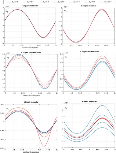
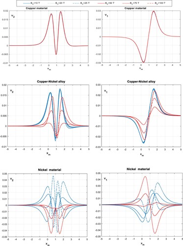
Figure 2 demonstrates a numerical example of solving the direct problem, specifically the surface diffraction waves (Rayleigh waves) on the upper surface of the magnetoelastic layer. This kind of waves depends on the scattering waves going out from the defect to the surface. A circular defect has been chosen like previous example. Figure 2 displays 6 diagrams of scattered surface waves with different values of the primary magnetic field versus a finite interval $[-5,5]$ of the upper surface. For the copper material, it is clear that all waves are identical over each other in one definite shape, where the diagram of $v_2$ pointed to the horizontal location of the defect in the layer since $x_c=d/2=1$. While the diagram of $v_2$ represents a bulk of symmetric waves about the vertical axis $y_c=d/2=1$ as one wave. The waves' behavior over the nickel material surface, for each magnetic value, takes a rosy form, unlike the behavior of waves in the copper material or in the copper-nickel alloy is. The waves in the alloy are arranged in an ascending form or descending when ${\mu }_r>25$ Tesla. This proves again that the sensitive property of the relative permeability factor ${\mu }_r$ is valid for the surface waves too. Finally, this property agrees with the previous conclusion reported by Lee et al. [10].

Figure 2. The diffracted surface waves from a defect centred at (1, 1), in three conductive materials, under various strengths of the magnetic field, versus a finite interval on the upper surface.

Notice that, in the case of non-smooth defects or crack with jagged edges, there are two techniques developed to solve such problems. The first technique depends on modeling the roughness edge of the crack as a smooth edge, or polygonal line, that has been randomly perturbed. The rough edge L will be close to a smooth curve $L_0$ (the nonperturbed crack edge) whose radii of curvature are far larger than the lengths of segments of L. However, the other technique based on modeling the roughness contour of the defect as a nonconvex obstacle with a piecewise smooth boundary L having M corner points. For this contour, we construct a convex hull $L_0$ (i.e. the smallest convex contour containing L), such that $L_m(L\cap L_0)$ is the common segments of contours L and $L_0$, and ${\ell }_m$ are the segments that belong only to $L(\bigcup _{m=1}^M{\ell }_m=L\mathrm{\setminus }{L}_0)$.

The problem is usually solved in two steps. Firstly, an approximate expression for the scattered field in the form of an integral over the crack edge should be derived. To this end, we use a version of the Geometrical Theory of Diffraction (GTD) for calculating the edge waves excited by each segment of the rough crack edge. Secondly, we perform an analytic treatment of statistics by using the Kirchhoff approximation. For more details, see references [44,45].

We conclude that, for all rough contours that can be represented by two parametric equations, the proposed inversion algorithm will be more efficient, even for defects having sharp corners, than the GTD method in detection. At least the location of those defects can be determined.

Figure 3 shows new kinds of patterns of direct solutions (the scattered waves) from various geometrical shapes; for example, the elliptical shapes with inclined angles θ, $\ell :\left\{\begin{array}{c}{y}_1=x_c+\rho \left(\theta \right)\cos \phi ,y_2=y_c+\rho \left(\theta \right)\sin \phi ,\\ \rho \left(\theta \right)=ab/\sqrt{a^2{\sin }^2(\theta +\phi )+b^2{\cos }^2(\theta +\phi )}\end{array},0\le \phi \le 2\pi \right.$the epicycloid with m cusps (m sharp corners), m is positive integer, $\ell :\left\{\begin{array}{c}{y}_1=x_c+(m+1)r\cos \phi -r\cos \left(\right(m+1\left)\phi \right)\\ y_2=y_c+(m+1)r\sin \phi -r\sin \left(\right(m+1\left)\phi \right),\end{array},0\le \phi \le 2\pi \right.$and the rectangle with rounded corners: $\ell :\left\{\begin{array}{l}{y}_1=x_c+\varrho \left(\psi \right)\cos \phi ,\\ y_2=y_c+\varrho \left(\psi \right)\sin \phi ,\\ \varrho \left(\psi \right)={\left[{\left(\frac{\cos \psi }{a}\right)}^m+{\left(\frac{\sin \psi }{b}\right)}^m\right]}^{(-1/m)}.\end{array}0\le \psi \le 2\pi .\right.$

Figure 3. (a) the solution of the direct problem for inclined elliptical defects with three angles $\theta =0,\pi /2,3\pi /4$ in Copper-Nickel material, (b) the solution for smooth rectangular defects with rounded corners in Nickel material, (c) the solution for smooth epicycloidal defects with having different cross-sections.

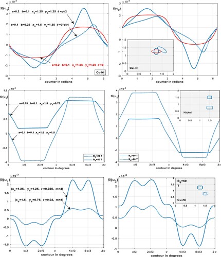
Figure 3 shows several patterns of the scattered field from various defects, in the shape of inclined ellipses with angle $\pi /2,3\pi /4$, versus the regular elliptic shape. However, the second graph of Figure 3 refers to the scattered waves from a square and rectangle, in different locations, in a Nickel layer, which subjected to varying strengths of a magnetic field. Moreover, patterns of the scattered waves from defects with sharp corners, epicycloid with different sizes, each have four cusps, in a Copper-Nickel layer under a moderate strength of the magnetic field.

4. The inverse problem and applications

Formulation of the geometrical inverse problem in solid mechanics aims to detect or identify the location and size of a defect or crack in a layer or solid medium according to output data measured from the medium. Many inverse problems in the elastic layered medium are investigated in previous works [33–35]. Another aim of the inverse problem formulation in magnetoelasticity is to predict the external magnetic field surrounded the medium that is valid if the outgoing diffraction waves from defects, inside this medium, could be measured over its outer surface.

Theoretically, if the problem is solved numerically, then the displacement Field $\left(u_1\right(y),u_2(y\left)\right)$ will be calculated over the contour ℓ. Furthermore, the scattered surface field will be easy to determine. However, in practice, such data is evaluated by measuring the amplitude of the free oscillations. Here, we used a numerical technique for solving the inverse problem of an oscillating medium having defects, based on the amplitude of the free surface oscillations over a certain finite interval $\mathrm{\Gamma }=[c_0,d_0]$ of the upper surface. Precisely, this diffraction surface field $(v_1,v_2)$ could be determined numerically if the integral Equations (40(40) $\begin{array}{rl}& \frac{u_m\left(x\right)}{2}+{\int }_{\ell }{\mathrm{\Sigma }}_{jk}^{\left(m\right)}(y,x)n_k{u}_j\left(y\right)\mathrm{d}{l}_y=f_m\left(x\right),x\in \ell \end{array}$(40) ), (41(41) $\begin{array}{rl}& \frac{u_m\left(x\right)}{2}+{\int }_{\ell }{\mathbb{T}}_j^{\left(m\right)}(y,x)u_j\left(y\right)\mathrm{d}{l}_y=g_m\left(x\right),x\in \ell ,\end{array}$(41) ) are solved for both magnetically impermeable and permeable layers, respectively. Therefore, we can formulate the surface field equations as follows (46) $\begin{array}{rl}& \left(\begin{array}{c}{v}_1\left(\zeta \right)\\ v_2\left(\zeta \right)\end{array}\right)=-{\int }_{\ell }\left(\begin{array}{cc}{K}_1^{\left(1\right)}(y,\zeta )& K_2^{\left(1\right)}(y,\zeta )\\ K_1^{\left(2\right)}(y,\zeta )& K_2^{\left(2\right)}(y,\zeta )\end{array}\right)\left(\begin{array}{c}{u}_1\left(y\right)\\ u_2\left(y\right)\end{array}\right)\mathrm{d}{\ell }_y,y\in \ell \end{array}$(46) (47) $\begin{array}{rl}& \left(\begin{array}{c}{v}_1\left(\zeta \right)\\ v_2\left(\zeta \right)\end{array}\right)=-{\int }_{\ell }\left(\begin{array}{cc}{K}_1^{\star \left(1\right)}(y,\zeta )& K_2^{\star \left(1\right)}(y,\zeta )\\ K_{1)}^{\star \left(2\right)}(y,\zeta )& K_2^{\star \left(2\right)}(y,\zeta )\end{array}\right)\left(\begin{array}{c}{u}_1\left(y\right)\\ u_2\left(y\right)\end{array}\right)\mathrm{d}{\ell }_y-\left(\begin{array}{c}{g}_1^{\star }\left(\zeta \right)\\ g_2^{\star }\left(\zeta \right)\end{array}\right)\end{array}$(47) where (48) $\begin{array}{l}{g}_m^{\star }\left(\zeta \right)=B_0{\int }_{\ell }{h}^0\left(y\right){\delta }_{ik}{U}_i^{\left(m\right)}(y,\zeta )n_k\left(y\right)\mathrm{d}{\ell }_y,i,k,m=1,2,\\ \zeta \in \mathrm{\Gamma }=\left\{\right({\zeta }_1,{\zeta }_2):c_0\le {\zeta }_1\le d_0,{\zeta }_2=d\},y\in \ell .\end{array}$(48) Notice, in the above equation, the term $f_m$ is omitted since the amplitude of surface wave $v_m\left(\zeta \right)$ is given in its relative form when compared with the analogous amplitude of a medium that doesn't have any defect inside. Here, the kernels of integrals have regularized as mentioned previously in Equation (40(40) $\begin{array}{rl}& \frac{u_m\left(x\right)}{2}+{\int }_{\ell }{\mathrm{\Sigma }}_{jk}^{\left(m\right)}(y,x)n_k{u}_j\left(y\right)\mathrm{d}{l}_y=f_m\left(x\right),x\in \ell \end{array}$(40) ) and (41(41) $\begin{array}{rl}& \frac{u_m\left(x\right)}{2}+{\int }_{\ell }{\mathbb{T}}_j^{\left(m\right)}(y,x)u_j\left(y\right)\mathrm{d}{l}_y=g_m\left(x\right),x\in \ell ,\end{array}$(41) ).

In Figure 2, we have computed the surface wave field $(v_1,v_2)$ over the interval $\mathrm{\Gamma }=[c_0,d_0]=[-5,5]$ by dividing this interval into M = 32 points, such that; ${\zeta }_t=c_0+q{h}_{\zeta },h_{\zeta }=(d_0-c_0)/M,q=1,2,\dots M$, where the location of the force point $y_0$ is excluded from that interval.

The identification of the defect's image in elasticity is to find its contour's parameters ℓ if the input data are known. Specifically, if the surface function $v_m\left(\zeta \right)$ is known, then the identification process is possible at least with a certain random noisy. Then the parameters of the defect's contour can be determined. Here, it should be noted that not only contour ℓ is unknown but also the field functions $(u_1,u_2)$ in Equation (47(47) $\begin{array}{rl}& \left(\begin{array}{c}{v}_1\left(\zeta \right)\\ v_2\left(\zeta \right)\end{array}\right)=-{\int }_{\ell }\left(\begin{array}{cc}{K}_1^{\star \left(1\right)}(y,\zeta )& K_2^{\star \left(1\right)}(y,\zeta )\\ K_{1)}^{\star \left(2\right)}(y,\zeta )& K_2^{\star \left(2\right)}(y,\zeta )\end{array}\right)\left(\begin{array}{c}{u}_1\left(y\right)\\ u_2\left(y\right)\end{array}\right)\mathrm{d}{\ell }_y-\left(\begin{array}{c}{g}_1^{\star }\left(\zeta \right)\\ g_2^{\star }\left(\zeta \right)\end{array}\right)\end{array}$(47) ) and (48(48) $\begin{array}{l}{g}_m^{\star }\left(\zeta \right)=B_0{\int }_{\ell }{h}^0\left(y\right){\delta }_{ik}{U}_i^{\left(m\right)}(y,\zeta )n_k\left(y\right)\mathrm{d}{\ell }_y,i,k,m=1,2,\\ \zeta \in \mathrm{\Gamma }=\left\{\right({\zeta }_1,{\zeta }_2):c_0\le {\zeta }_1\le d_0,{\zeta }_2=d\},y\in \ell .\end{array}$(48) ) are unknown. Therefore, we can describe, in a mathematical view, the inverse problem is non-linear relative to the parametric equations of this contour ℓ. Moreover, we predict that the external magnetic field and the nature of the checked materials will play a sensitivity rule in the identification and localization of the defect and stability or instability of the algorithm of detection.

It should be noted that the inverse problem is nonlinear and well-posed with respect to the parametric equations of the contour ℓ. Generally, the initial problem in its continuous formulation is ill-posed. However, for an object, regular or irregular with finite parameters, the problem will be finite-dimensional, furthermore well-posed, the proof in reference [45]. Numerically, this leads to a practical instability in the case of the input data with noise. The question of existence and uniqueness investigated in previous work [46], so this scope is out of the present study. Moreover, we have developed a numerical technique, not only to detect the defect's parameters but also to predict the applied magnetic field to the medium. Now, let us arrange three steps describing the most efficient technique of detection, as follows:

•	Firstly, the basic boundary integral equation is written as an operator equation. The operator has an inverse if the contour ℓ of the defect is known. Therefore, for magnetically permeable defect, we can write the operator Equation (46(46) $\begin{array}{rl}& \left(\begin{array}{c}{v}_1\left(\zeta \right)\\ v_2\left(\zeta \right)\end{array}\right)=-{\int }_{\ell }\left(\begin{array}{cc}{K}_1^{\left(1\right)}(y,\zeta )& K_2^{\left(1\right)}(y,\zeta )\\ K_1^{\left(2\right)}(y,\zeta )& K_2^{\left(2\right)}(y,\zeta )\end{array}\right)\left(\begin{array}{c}{u}_1\left(y\right)\\ u_2\left(y\right)\end{array}\right)\mathrm{d}{\ell }_y,y\in \ell \end{array}$(46) ) as follows (49) $\mathit{u}={\mathit{B}}^{-1}\mathit{g},$(49) where both of the inverse operator ${\mathit{B}}^{-1}={\mathit{B}}^{-1}(a,b,x_c,y_c)$, and the term $g_m^{\star }$ depend on the unknown four geometric parameters $(a,b,x_c,y_c)$ of the elliptic contour ℓ.
•	Let us rewrite symbolically Equation (48(48) $\begin{array}{l}{g}_m^{\star }\left(\zeta \right)=B_0{\int }_{\ell }{h}^0\left(y\right){\delta }_{ik}{U}_i^{\left(m\right)}(y,\zeta )n_k\left(y\right)\mathrm{d}{\ell }_y,i,k,m=1,2,\\ \zeta \in \mathrm{\Gamma }=\left\{\right({\zeta }_1,{\zeta }_2):c_0\le {\zeta }_1\le d_0,{\zeta }_2=d\},y\in \ell .\end{array}$(48) ) in an operator form, having the input data function $v_m\left(\zeta \right)$ on the left-hand side. Then by substituting of Equation (50(50) $v\left(\zeta \right)=\left[\hat{K}({\mathit{B}}^{-1}\right(a,b,x_c,y_c)\mathit{g})-g^{\star }(a,b,x_c,y_c\left)\right]\left(\zeta \right),\zeta \in \mathrm{\Gamma }.$(50) ) in that operator relation, one obtains: (50) $v\left(\zeta \right)=\left[\hat{K}({\mathit{B}}^{-1}\right(a,b,x_c,y_c)\mathit{g})-g^{\star }(a,b,x_c,y_c\left)\right]\left(\zeta \right),\zeta \in \mathrm{\Gamma }.$(50) If the amplitude of the surface field $v\left(\zeta \right)$ is known exactly, as a result of the direct problem, then the solution of the Equation (51(51) $v\left({\zeta }_q\right)=\left[\hat{K}({\mathit{B}}^{-1}\right(a,b,x_c,y_c)\mathit{g})-g^{\star }(a,b,x_c,y_c\left)\right]\left({\zeta }_q\right),q=1,2,\dots ,M.$(51) ) should match with the real contour ℓ. Now, the question about how the numerical algorithm of identification work, or how it will reconstruct the four geometrical parameters without known a priori the contour ℓ especially when the input data perturbed with random noise. Thus, the introduced algorithm for restoring the defect should be stable relative to small disturbances in the input data.
•	Let us consider the surface field $v_m\left(\zeta \right)$ in Equation (51(51) $v\left({\zeta }_q\right)=\left[\hat{K}({\mathit{B}}^{-1}\right(a,b,x_c,y_c)\mathit{g})-g^{\star }(a,b,x_c,y_c\left)\right]\left({\zeta }_q\right),q=1,2,\dots ,M.$(51) ), is known in a discrete set of nodes ${\zeta }_q\in \mathrm{\Gamma },(q=1,2,\dots ,M)$. Then we can write: (51) $v\left({\zeta }_q\right)=\left[\hat{K}({\mathit{B}}^{-1}\right(a,b,x_c,y_c)\mathit{g})-g^{\star }(a,b,x_c,y_c\left)\right]\left({\zeta }_q\right),q=1,2,\dots ,M.$(51) Based on a proposed numerical algorithm which we have developed in previous works [33–35], the solution of Equation (52(52) $\begin{array}{rl}\mathrm{\Omega }(a,b,x_c,y_c)& =\parallel \sum _{j=1}^N[\hat{K}({\mathit{B}}^{-1}(a,b,x_c,y_c)\mathit{g})-g^{\star }(a,b,x_c,y_c)]\left({\zeta }_q\right)-v_m\left({\zeta }_q\right){\parallel }^2\\ & =\sum _{q=1}^M{\left\{\sum _{j=1}^N[\hat{K}({\mathit{B}}^{-1}(a,b,x_c,y_c)\mathit{g})-g^{\star }(a,b,x_c,y_c)]\left({\zeta }_q\right)-v_m\left({\zeta }_q\right)\right\}}^2,\end{array}$(52) ) depends on minimizing the following discrepancy functional Ω: (52) $\begin{array}{rl}\mathrm{\Omega }(a,b,x_c,y_c)& =\parallel \sum _{j=1}^N[\hat{K}({\mathit{B}}^{-1}(a,b,x_c,y_c)\mathit{g})-g^{\star }(a,b,x_c,y_c)]\left({\zeta }_q\right)-v_m\left({\zeta }_q\right){\parallel }^2\\ & =\sum _{q=1}^M{\left\{\sum _{j=1}^N[\hat{K}({\mathit{B}}^{-1}(a,b,x_c,y_c)\mathit{g})-g^{\star }(a,b,x_c,y_c)]\left({\zeta }_q\right)-v_m\left({\zeta }_q\right)\right\}}^2,\end{array}$(52) Here, the inverse problem is classified as a non-linear unconstrained optimization problem. So we have used the BFGS method which is one of the most popular quasi-Newton iterative methods [47]. This method can be described as an effective, robust, quadratically convergent method and provides a sort of iterative regularization that gives an additional stability condition to the identification algorithm.

Here, our aim to check the efficiency of the algorithm of reconstruction for identifying defect with complex geometrical shapes as well as elliptic contours. The validation occurs as the discrepancy functional Ω approaches to zero. Notice that, the global minimum of the functional Ω is automatically achieved if the input data used exactly in the functional Ω. Hence $min\left(\mathrm{\Omega }\right)=0$, implies the restored data coincide to the real contour ℓ.

In the following reconstruction examples, we have used the MATLAB's minimization toolbox function ”fminunc” uses a line search based on the BFGS method. For all examples below, we have chosen the interval $\mathrm{\Gamma }=[-5,5]$ on the upper surface of the layer and then split it by M = 32 points to measure the free surface oscillations. Those oscillations will be the input data for the detection process of any defect in the layer. Firstly, let us define the following essential criteria of reconstructions by the ratios: $\begin{array}{rl}{ϵ}_a& =(a^{\ast }-a)/a,{ϵ}_b=(b^{\ast }-b)/b,{ϵ}_{x_c}=(x_c^{\ast }-x_c)/x_c,\\ {ϵ}_{y_c}& =(y_c^{\ast }-y_c)/y_c,{ϵ}_A=\left(\right(ab{)}^{\ast }-ab)/ab,{ϵ}_B=(B^{\ast }-B_0)/B_0,\end{array}$which are the so-called ‘Relative errors ${ϵ}_i$’ of the reconstruction process for a defect in layer while ${ϵ}_B$ is the relative error of applied magnetic field.

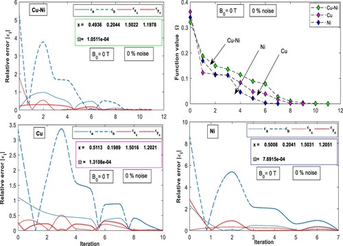
Figure 4 demonstrates an example of reconstructing defects in an elastic layer oscillating with angular frequency $\omega =20\pi$, in the case of non-magnetic field, i.e. B=0. For minimizing the discrepancy functional Ω and the thickness of the layer h = 2, we have used the initial guess point $z^0=(0.1,0.1,1,1)$ in the middle layer. The figure illustrates the pure nature of these conductive materials on the algorithm of detection without the effect of the magnetic field with zero noise. Moreover, the diagram of ”Function value Ω” shows that the considered materials are semi-identical in the path of minimizing the discrepancy functional Ω, and the number of iterations. However, the diagrams of the relative errors display the four paths of the relative errors of the restored geometrical parameters of the defect and the real contour's parameters $\ell (a,b,x_c,y_c)=(0.5,0.2,1.5,1.2)$ for each material in zero noise. Having noted the graphs of Figure 3, it is to be observed that, in all materials the path of ${ϵ}_b$ is so long when converges to zero compared to the paths of other parameters.

Figure 4. The relative error criterion $|{ϵ}_i|$ of ellipse parameters, in three different materials in the absence of the magnetic field, with the corresponding restored vector x of the parameters.

Figures 5–7 show the effect of the magnetic field on the algorithm of detection in the presence of different levels of noise. Figure 5 reflects a comparison that indicates the effect of two different noise present on the paths of the relative errors of geometrical parameters of a defect in the copper-nickel alloy. The applied initial magnetic field on the layer is chosen to be $B_0=50$ tesla, with defect's parameters $\ell (a,b,x_c,y_c)=(0.5,0.2,1.5,1.2)$. Diagrams of Figures 5–7 show that the efficiency of the algorithm of detection is perfect even if $20\mathrm{\%}$ noisy data are used. The size of the real contour is larger compared to the initial object of detection, which is another reason for the efficiency of the proposed algorithm. However, Figure 6 is constructing to show the effect of the high relative permeability on the detection algorithm under moderate magnetic field strength $B_0=50$ tesla for different noisy data, versus the number of iterations. There is no difference between the noise levels in Figure 6 except the number of iterations that increased. But it causes high values of the objective function $(\mathrm{\Omega }=92,78)$ compared to the values of Figure 5 $(\mathrm{\Omega }=1.6,1.35)$.

Figure 5. (a) The minimizing path of the discrepancy functional Ω in two noise levels, (b) the relative error criterion $|{ϵ}_i|$ of ellipse parameters in a Copper-Nickel alloy, subjected to a magnetic field of strength 50 Tesla, with the corresponding restored vector x of the parameters.

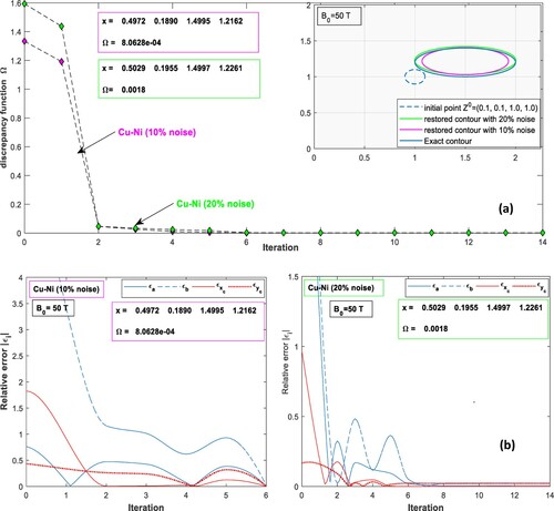
Figure 6. (a) The minimizing path of the discrepancy functional Ω in two noise levels, (b) the relative error criterion $|{ϵ}_i|$ of ellipse parameters in Nickel layer, subjected to a magnetic field of strength 50 Tesla, versus the number of iterations, with the corresponding restored vector x of the parameters.

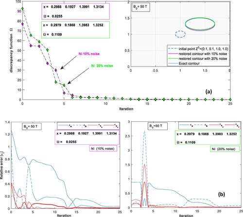
Figure 7. (a) The minimizing path of the discrepancy functional Ω in two noise levels, (b) the relative error criterion $|{ϵ}_i|$ of ellipse parameters, close to bottom of a Copper layer subjected to a magnetic field of strength 100 Tesla, with the corresponding restored vector x of the parameters.

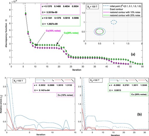
Figure 7 displays a reconstruction process of a small elliptic defect, located near the bottom of a copper layer, while the layer subjected to a magnetic field $B_0=100$ tesla, and two noisy levels of the input data. The paths of functions evaluation are approximately identical except for the number of iterations that increased to double. The proposed algorithm extremely succeeded to find the defect in Figure 6 exactly, compared to Figure 7, where the size of the restored object is found smaller than real defect but in the same location.

Figures 8–11 reflect the validity of the detection algorithm to restore complex geometrical shapes in the magnetoelastic layer. Figure 8 shows the reconstruction process of two defects, in the shape of elliptic contour with inclined angles $\theta =\pi /2,3\pi /4$. The discrepancy functional works on five parameters, the fifth one is the inclined angle θ, which plays a distinctive rule for restoring images. For example, in Figure 8(a) shows the ellipses are coinciding, however, the restored angles are different from the real contour, which has an angle $\theta =\pi /2$. It seems a different defect is restored, since the output data show the ratio (a/b) of the restored is the inverse value of the real one, and the new principal axis inclined approximately by the angle $\theta =0$. Also, the same result of identical is repeated in Figure 8(b), the real ellipse one with an angle $\theta =3\pi /4$, while the restored has a different one. Consequently, the results represent well-reconstructed images for the same defect, especially, when the principal axis of the defect inclines on the horizontal.

Figure 8. Three noisy levels of minimizing the discrepancy functional Ω, for reconstructing two elliptical defects with inclined angles $\mathrm{\Theta }=\pi /2,3\pi /4$ in a Copper-Nickel layer subjected to an initial magnetic field B${}_0$=50 Tesla, with the corresponding restored vector x of the parameters.

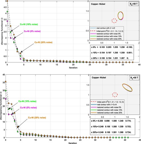
Figure 9 illustrates the process of restoring defects with contours, in the shape of square and rectangle having rounded corners, in a Nickel layer. It is clear that, as the object close to the surface, the precision of the detection tends to be low with increasing the noise levels. Figure 10 displays a new technique of restoring defects that have sharp corners, for example, an epicycloid with 4 cusps. Two different guess shapes are used to restore the epicycloidal defects. The results refer to, the precision of the reconstruction process is high relative to the rectangular shape more than ellipse.

Figure 9. Three noisy levels of the minimizing the discrepancy functional Ω for reconstructing two defects in the shape of a square and rectangle with rounded corners, in a Nickel layer subjected to two different magnetic fields B${}_0$= 20, 50 Tesla, with the corresponding restored vector x of the parameters.

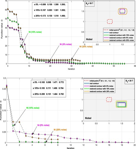
Figure 10. Three noisy levels of minimizing the discrepancy functional Ω for reconstructing two epicycloidal defects, in a Copper-Nickel layer subjected to magnetic field B${}_0$= 50 Tesla, by using rectangular and elliptical shapes, with the corresponding restored vector x of the parameters.

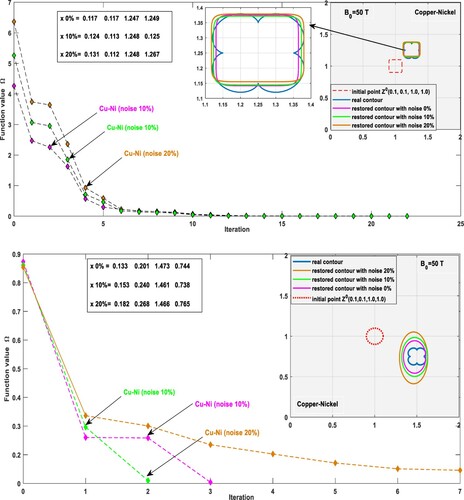
Figure 11. The reconstructing images of an irregular shape with 5 vertices by using elliptical shapes, at different frequencies, in a Copper-Nickel layer subjected to magnetic field B${}_0$= 10 Tesla.

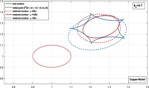
Figure 11 displays the reconstruction process of an irregular defect, with five vertices, (53) $\ell :\left\{\begin{array}{c}{y}_1=x_c+(a-b)\cos \phi -b\cos \left(\right(k-1\left)\phi \right),`\\ y_2=y_c+(a-b)\sin \phi +b\sin \left(\right(k-1\left)\phi \right),k=a/b\end{array}\right.$(53) in a Copper-Nickel layer, by using elliptical shapes, at different frequencies. In low magnetic field, the figure shows the efficiency of the algorithm of detection increases as the frequency decreases. It proves the algorithm is useful at least to found exactly the location of any closed shapes, even they are irregular and having vertices.

Some numerical examples of detection are demonstrated in Tables 2 and 3 for the considered materials. Table 2 displays some reconstruction results for defects in magnetically permeable case to study the detection precision versus the applied magnetic field and noise levels. In this table, we assumed a defect that has $\ell (0.3,0.2,1.4,1.3)$ in all materials subjected to magnetic field varies from 20 to 100 tesla, to study the inverse problem parameters by using the initial guess point $z^0(0.1,0.1,1,1)$ in the presence of two different levels of noise.

Table 2. Examples of the reconstruction in three different materials, in two noisy cases, under a magnetic field with various strengths versus the relative error criteria.

Material	Noise	B${}_0$	Iteration	${ϵ}_a$%	${ϵ}_b$ %	${ϵ}_{xc}$%	${ϵ}_{yc}$ %	${ϵ}_A$ %
Nickel	5%	20	25	0.20	1.25	0	0.40	1.95
		50	26	0.20	1.90	0.03	0.53	2.10
		100	46	2.4	3. 2	4.5	3.25	4.25
	20%	20	18	0.37	2.50	0.01	1.54	2.88
		50	25	0.70	6.60	0.12	1.94	7.25
		100	81	8.15	10.2	10.31	11.02	18.40
			High relative errors since Ω doesn't converges to zero
Copper Nickel	5%	20	24	0.43	2.25	0.036	0.54	1.73
		50	25	1.50	0.27	0	0.48	1.76
		100	25	6.7	3.60	0	0.62	4.24
	20%	20	23	1.57	8.05	0.14	1.96	6.61
		50	23	0.53	4.85	0.007	1.75	5.36
		100	27	1.97	10.50	0.014	2.13	8.26
Copper	5%	20	24	0.37	2.05	0.05	0.54	1.29
		50	22	0.40	2.10	0.042	0.54	1.31
		100	25	0.50	2.20	0.028	0.54	1.71
	20%	20	25	1.47	7.25	0.18	1.98	4.89
		50	25	1.50	7.35	0.16	1.98	4.96
		100	26	1.77	7.95	0.10	1.98	6.32

Table 3. Examples of prediction of the external magnetic field applied upon a copper layer having different defects.

Material	ℓ (a, b, x${}_c$, y${}_c$)	B${}_0$	Noise	Iteration	Ω value	B*	${ϵ}_B$ %
Copper	(0.2, 0.15, 1.25, 1.20)	125	0%	5	1.9349e-06	122.680	1.71
			10%	10	2.8336e-04	129.7911	3.84
			20%	17	0.00435	133.3201	6.64
	(0.05, 0.05, 1.50, 1.30)	125	0%	8	2.4910e-06	124.866	0.12
			10%	24	1.5336e-04	121. 646	2.72
			20%	17	0.001472	119.3645	4.51
	(0.5, 0.5, 1.0, 1.0)	125	0%	4	1.4628e-06	129.7911	3.84
			10%	9	6.5336e-04	139.105	11.28
			20%	24	0.61252	145	16

For the material, we remarked that the relative error levels are rising as the magnetic field and the noise in the input data increase until $B_0$ =100 tesla whereas the algorithm failed to approaches zero with $20\mathrm{\%}$ noise level. Which in turn proves that the magnetic field affects negatively the identification process for materials with a high magnetic permeability factor, especially when the magnetic field and noise levels increase. Although the algorithm succeeded in the copper material and copper-nickel alloy even when the magnetic field increases.

As for Table 3, we present a different inverse problem to predict the external magnetic field, which applied to a copper layer contains various defects. The table displays defect locates in different locations and sizes. The algorithm of detection is checked under random noise, in magnetically impermeable case, to study its stability by using the relative error ratio of ${ϵ}_B$. In this algorithm, the contour ℓ is known in both direct and inverse problem however, the input data is assumed according to the magnetic field is known in the direct problem. The magnetic field that is only unknown in the inverse problem. So we have proposed a different algorithm for identifying by using the MATLAB's minimization toolbox function ‘lsqnonlin’ with an initial guess field $b_0=$ 25, lower bounds lb= 0, and upper bounds ub= 500. The algorithm is so valid for the small defects even for high random noise level, but its accuracy gradually decreases as the size of defect increases and the noise level.

Conclusion

The main results of studying direct and inverse scattering problem by various defects in the magnetoelastic layer have shown that:

•	A direct scattering in-plane problem from defects in a conductive magnetoelastic layer investigated analytically.
•	The direct diffraction problem is reduced to a coupled system of boundary integral equation (BIEs), over the boundary contour of the defect, based on the constructed Greens' functions.
•	An efficient numerical technique for solving a coupled system of BIEs, based on the boundary element method, is applied. A series of numerical examples representing the solution to the direct problem to defects of elliptic and complex geometrical shapes, for magnetically permeable or impermeable defects, in different materials subjected to a magnetic field, is presented.
•	The relative permeability factor ${\mu }_r$ has a high sensitivity rule, which is founded on the density distribution of diffraction waves that may be reliable when the value of this factor changes.
•	A numerical detection algorithm to solve the inverse scattering problems, for various geometrical defects, in a conductive magnetoelastic layer is developed, based on minimizing the discrepancy functional in the parameters of defects. Moreover, even with input data having randomly distributed errors, the algorithm of detection remains stable and works well.
•	The detection algorithm is more sensitive to restore the geometrical parameters of the defect, even if the object placed near the bottom of the layer.
•	The results showed that the magnetic field affects negatively on the identification algorithm, specifically for the high magnetic permeability material (Nickel material), especially when the eternal magnetic field increases.
•	The work presents a numerical example for a special inverse scattering problem to predict the external magnetic field over a copper layer contains defects of various sizes.

Disclosure statement

No potential conflict of interest was reported by the author(s).

Appendices

Appendix 1

From the following algebraic system the unknown constants $C_i^{\left(m\right)}\left(s\right)$ are determined. For m=1: $\left\{\begin{array}{l}{C}_1^{\left(1\right)}+\left(\frac{{\gamma }_s}{is}\right)C_4^{\left(1\right)}=g_{11}\\ \left(\frac{-{\gamma }_1}{is}\right)C_2^{\left(1\right)}+C_3^{\left(1\right)}=g_{12}\\ (2{\gamma }_1\sinh ({\gamma }_{1}d\left)\right)C_1^{\left(1\right)}+(2{\gamma }_1\cosh ({\gamma }_{1}d\left)\right)C_2^{\left(1\right)}+\left(\frac{({\gamma }_s^2+s^2)}{is}\cosh \left({\gamma }_{s}d\right)\right)C_3^{\left(1\right)}+\\ \left(\frac{({\gamma }_s^2+s^2)}{is}\sinh \left({\gamma }_{s}d\right)\right)C_4^{\left(1\right)}=g_{13}\\ \left(\frac{-{\gamma }_1^2+s^2(1-2c_{\eta }^2)}{is}\cosh \left({\gamma }_{1}d\right)\right)C_1^{\left(1\right)}+\left(\frac{-{\gamma }_1^2+s^2(1-2c_{\eta }^2)}{is}\sinh \left({\gamma }_{1}d\right)\right)C_2^{\left(1\right)}\\ +(2c_{\eta }^2{\gamma }_s\sinh ({\gamma }_{s}d\left)\right)C_3^{\left(1\right)}+(2c_{\eta }^2{\gamma }_s\cosh ({\gamma }_{s}d\left)\right)C_4^{\left(1\right)}=g_{14},\end{array}\right.$where $\left\{\begin{array}{l}{g}_{11}=\frac{-{\mathrm{e}}^{is{\xi }_1}}{2\rho {\omega }^2}\left\{\frac{s^2}{{\gamma }_1}{\mathrm{e}}^{-{\gamma }_1{\xi }_2}-{\gamma }_s{\mathrm{e}}^{-{\gamma }_s{\xi }_2}\right\}\\ g_{12}=\frac{{\mathrm{e}}^{is{\xi }_1}}{2\rho {\omega }^2}\left\{{\mathrm{e}}^{-{\gamma }_1{\xi }_2}-{\mathrm{e}}^{-{\gamma }_s{\xi }_2}\right\}\\ g_{13}=\frac{{\mathrm{e}}^{is{\xi }_1}}{2\rho {\omega }^2}\left\{-2s^2{\mathrm{e}}^{-{\gamma }_1{\xi }_2}-({\gamma }_s^2+s^2){\mathrm{e}}^{-{\gamma }_s{\xi }_2}\right\}\\ g_{14}=\frac{\left(is\right){\mathrm{e}}^{is{\xi }_1}}{2\rho {\omega }^2}\left\{\frac{-{\gamma }_1^2+s^2(1-2c_{\eta }^2)}{{\gamma }_1}{\mathrm{e}}^{-{\gamma }_1{\xi }_2}+2c_{\eta }^2{\gamma }_s{\mathrm{e}}^{-{\gamma }_s{\xi }_2}\right\}\end{array}\right.$One can determine the constants $C_i^{\left(1\right)}$ by using Cramer's rule ${\displaystyle C_i^{\left(1\right)}=\frac{{\mathrm{\Delta }}_i(s,\xi )}{\mathrm{\Delta }\left(s\right)}}$, i=1,2,3,4, where $\mathrm{\Delta }\left(s\right)$ is the basic determinant of the above system and is expressed in the following form: $\left\{\begin{array}{l}\mathrm{\Delta }\left(s\right)=\frac{2{\gamma }_1{\gamma }_s}{s^2}({\gamma }_p^2-{\gamma }_1^2)+{\gamma }_1{\gamma }_s\cosh \left({\gamma }_{s}d\right)\cosh \left({\gamma }_{1}d\right)[-4s^2+\frac{1}{s^4}({\gamma }_s^2+s^2\left)\right(-{\gamma }_1^2\\ +s^2(1-2c_{\eta }^2)\left)\right]+\frac{1}{s^2}\sinh \left({\gamma }_{s}d\right)\sinh \left({\gamma }_{1}d\right)\left[4c_{\eta }^2{\gamma }_1^2{\gamma }_s^2-({\gamma }_s^2+s^2)(-{\gamma }_1^2+s^2(1-2c_{\eta }^2\left)\right)\right].\end{array}\right.$The final expression of Green's functions is constructed directly after finding the constants $C_i^{\left(m\right)}$ and applying the Fourier inversion formula on the parameter s. The inversion integral formulae are treated by the quadrature numerical method.

Appendix 2

• It is clear that both kernels of integral Equations (40(40) $\begin{array}{rl}& \frac{u_m\left(x\right)}{2}+{\int }_{\ell }{\mathrm{\Sigma }}_{jk}^{\left(m\right)}(y,x)n_k{u}_j\left(y\right)\mathrm{d}{l}_y=f_m\left(x\right),x\in \ell \end{array}$(40) ), (41(41) $\begin{array}{rl}& \frac{u_m\left(x\right)}{2}+{\int }_{\ell }{\mathbb{T}}_j^{\left(m\right)}(y,x)u_j\left(y\right)\mathrm{d}{l}_y=g_m\left(x\right),x\in \ell ,\end{array}$(41) ) contain Hankel functions ${\displaystyle H_0^{\left(1\right)}\left(kr\right)}$ and ${\displaystyle H_1^{\left(1\right)}\left(kr\right)}$, $r={\displaystyle \sqrt{(y_1-{\xi }_1{)}^2+(y_2-{\xi }_2{)}^2}}$. The regularization of the singularities in the kernels is carried out by specifying the the leading order singularity, subtracting from the integrals and evaluated separately.

• According to Ramesh [48], the integral systems which contain Hankel functions $H_0^{\left(1\right)}$ and $H_1^{\left(1\right)}$ as the kernels, the leading order behaviour of the singularity is $ln\left(kr\right)$ and 1/r, respectively, where these functions can be expressed as: $\left\{\begin{array}{l}{H}_0^{\left(1\right)}\left(kr\right)=-\ln \left(\frac{kr}{2}\right)\sum _{i=1}^{\mathrm{\infty }}{A}_i{r}^{2(i-1)}+\sum _{i=1}^{\mathrm{\infty }}{B}_i{r}^{2(i-1)};kr\le 2,\\ H_1^{\left(1\right)}\left(kr\right)=r\ln \left(\frac{kr}{2}\right)\sum _{i=1}^{\mathrm{\infty }}{D}_i{r}^{2(i-1)}+\frac{1}{r}\sum _{i=1}^{\mathrm{\infty }}{E}_i{r}^{2(i-1)};kr\le 2,\end{array}\right.$where $A_i,B_i,D_i$, and $E_i$ are known functions of k. Thus we explicitly separated the kernel in two parts one of Cauchy type of order $\mathcal{O}\left(1/r\right)$ and the other part is regular, as follows: $Ku\left(y\right)={\int }_{\ell }\left[K_0\right(y,\xi )+\overline{K}(y,\xi \left)\right]u\left(\xi \right)\mathrm{d}{l}_{\xi }$where $K_0(y,\xi )=\frac{1}{r}$The regular kernel $\overline{K}(y,\xi )$ is integrable by any quadrature formula. But the singular term is integrated analytically for each small segment of the interval $(0,2\pi )$,by using the polar transformation. To overcome the singularity in the integral equations which are resulted from coinciding of the external and internal nodes with each other. We introduce the following regularization technique as follows $y=(y_1,y_2)=\rho (\cos \phi ,\sin \phi ),\xi =({\xi }_1,{\xi }_2)=\rho (\cos \tau ,\sin \tau ),\mathrm{d}{l}_{\xi }=\rho \mathrm{d}\tau$Then $I={\int }_{\ell }\frac{u\left(\xi \right)}{\sqrt{(y_1-{\xi }_1{)}^2+(y_2-{\xi }_2{)}^2}}\mathrm{d}{l}_{\xi }={\int }_0^{2\pi }\frac{u\left(\tau \right)\mathrm{d}\tau }{\sqrt{(\cos \phi -\cos \tau {)}^2+(\sin \phi -\sin \tau {)}^2}}$This followed by dividing the interval $(0,2\pi )$ for the variables $\tau ,\phi$ to a number of small intervals of length $h_{\phi }$ and place $j^{th}$ node ${\tau }_j$ for both them just at the middle position $j^{th}$ subinterval. Then, we can apply the collocation technique $I\approx \frac{1}{\sqrt{2}}\sum _{j}u\left({\tau }_j\right){\int }_{{\tau }_j-h_{\varphi }/2}^{{\tau }_j+h_{\varphi }/2}\frac{\mathrm{d}\tau }{\sqrt{1-\cos (\phi -\tau )}}.$From the table of integrals we have ${\displaystyle \int \frac{\mathrm{d}\tau }{\sin \left(\tau /2\right)}=\ln (\tan (\tau /4\left)\right)}$, then one can formulate Cauchy singular integral in the following polar form: $I=\frac{1}{2}\sum _{j}u\left({\tau }_j\right)\ln \left[\frac{\tan \left[\right({\tau }_j+h_{\varphi }/2\left)/4\right]}{\tan \left[\right({\tau }_j-h_{\varphi }/2\left)/4\right]}\right].$

References

- Knopoff L. The interaction between elastic wave motions and a magnetic field in electrical conductors. J Geophys Res Solid Earth. 1995;60(4):441–456.
- Dunkin J, Eringen A. On the propagation of waves in an electromagnetic elastic solid. In J Eng Sci. 1963;1:461–495.
- Maugin G. Wave motion in magnetizable deformable solids. Int J Eng Sci. 1981;19:321–388.
- Das N, Bhattacharya S. Axisymmetric vibrations of orthotropic shells in a magnetic field. J Pure Appl Math. 1978;45(1):40–54.
- Gourakishwar O. Propagation of waves in magnetoelastic media. J Appl Phys. 1990;67(2):725–733.
- Andreou E, Dassios G. Dissipation of energy for magnetoelastic waves in conductive medium. Quarterly Appl Math. 1997;55:23–39.
- Kaliski S. Cerenkov generation of thermal waves for the wave equations of Thermo-Electro-Magneto-Elasticity. Proceedings of Symposium on Irreversible Aspects of Continuum Mechanics and Transfer of Physical Characteristics in Moving Fluids; Vienna: Springer; 1968.
- Eringen A, Maugin G. Electrodynamics of continua I. foundations and solid media. 2nd ed. New York: Springer; 1990. 47–90.
- Parton V, Kudryavtsev B. Electromagnetoelasticity, Piezoelectrics and electricity conducting solids. New York: Gordon and Breach Science Publisher; 1988. 10–100.
- Lee JS, Its EN. Propagation of Rayleigh waves in magneto-elastic media. J Appl Mech. 1992;59(4):812–818.
- Acharya DP, Maji C. Effect of surface stress on magneto-elastic surface waves in finitely conducting media. Acta Geophys. 2007;55(4):554–576.
- Narain S. Magneto-elastic Rayleigh waves on the surface of orthotropic cylinder of varying density. Defence Sci J. 1985;35(4):435–442.
- Acharya DP, Roy I. Magnetoelastic surface waves in electrically conducting fibre-reinforced media. Bullet Inst Math Academia Sinica (New Series). 2009;4(3):333–352.
- Lin CB, Lin HM. The magnetoelastic problem of cracks in bonded dissimilar materials. Int J Solids Struct. 2002;39:2807–2826.
- Rogowski B. Analysis of a penny-shaped crack in magneto-elastic medium. J Theoretical Appl Mech. 2009;47(1):143–159.
- Bagdasarian GY, Hasanian DJ. Magnetoelastic interaction between a soft ferromagnetic elastic half-plane with a crack and a constant magnetic field. Int J Solids Struct. 2002;37(38):5371–5383.
- Zhao SX, Lee KY. Interfacial crack problem in layered soft ferromagnetic materials in uniform magnetic field. Mech Res Commun. 2007;34(1):19–30.
- Wei L, Yapeng S, Daining F. Magnetoelastic coupling on soft ferromagnetic solids with an interface crack. Acta Mech. 2002;154(1-4):1–9.
- Hasebe N, Wang XF, Nakanishi H. On magnetoelastic problems of a plane with an arbitrarily shaped hole under stress and displacement boundary conditions. Quarterly J Mech Appl Math. 2007;60(4):423–442.
- Nowacki W. Two-dimensional problem of magnetothermoelasticity I. Bulletin De Academit Polonaise Des Science-Serie Des Science Techniques. 1965;13(5):485–493.
- Sladek V, Sladek J. Boundary integral method in magnetoelasticity. Int J Eng Sci. 1988;26(5):401–418.
- Fang X, Hua C, Huang W. Dynamic stress of a circular cavity buried in a semi-infinite functionally graded piezoelectric material subjected to shear waves. Europian J Mech-A/Solids. 2007;26:1016–1028.
- Fang X. Multiple scattering of electro-elastic waves from a buried cavity in a functionally graded piezoelectric material layer. Int J Solids Struct. 2008;45:5716–5729.
- Jinxi L, Xianglin L, Yongbin Z. Green's functions for anisotropic magnetoelectroelastic solids with an elliptical cavity or a crack. Int J Eng Sci. 2001;39:1405–1418.
- Qin Q. 2D Green's functions of defective magnetoelectroelastic solids under thermal loading. Eng Anal Boundary Elements. 2005;29:577–585.
- Lorenzi A, Priimenko V. Identification problem related to electro -magneto-elastic interactions. J Inverse Ill-posed Prob. 1996;4:115–143.
- Priimenko V, Vishnevskii M. An inverse problem of electromagnetoelasticity in the case of complete nonlinear interaction. J Inverse Ill-posed Prob. 2005;13(3):277–301.
- Priimenko V, Vishnevskii M. Mathematical problems of electromagnetoelastic interactions. Boletim Da Sociedade Paranaense De Matematica. 2007;25:55–66.
- Avdeev A, Soboleva O, Priimenko V. Inverse problem of Electro-magnetoelasticity: simultaneous determination of elastic and electromagnetic parameters. Proceedings of Symposium on Applied and Industrial Mathematics; Italy: Springer; 1998.
- Romanov V. A stability of the solution to a two-dimensional inverse problem of electrodynamics. Siberian Math J. 2003;44:659–670.
- Lu Y, Ye L, Su Z, et al. Artificial neural network (ANN)-based crack identification in aluminum plates with lamb wave signals. J Intelligent Mater Syst Struct. 2009;20(1):39–49.
- Hattori G, Saez A. Damage identification in multifield materials using neural networks. Inverse Prob Sci Eng. 2013;21(6):929–944.
- Sumbatyan M, Elmorabie KM, Brigante M. Detection of a buried void void in an elastic layer of constant thickness: the anti-plane problem: anti-Plane problem. Math Mech Solids. 2012;18(1):67–77.
- Elmorabie KM, Sumbatyan M. Detection of a single elliptic-shape buried Object in stratified elastic media: anti-Plane problem. Europian J Mech-A/Solids. 2013;37:1–7.
- Elmorabie KM, Sumbatyan M. Inverse diffraction problems for buried objects in the layered elastic media: the anti-plane problem. Inverse Prob Sci Eng. 2018;26(11):1540–1560.
- Elmorabie KM, Yahya R. The scattering waves from an object in an elastic-fluid layered structure. ZAMM-J Appl Math Mech/Zeitschrift Fur Angewandte Mathematik Und Mechanik. 2019;99(5):1–15.
- Achenbach J. Reciprocity in elastodynamics. UK: Cambridge University Press; 2003.
- Chattopadhyay A, Maugin GA. Diffraction of magnetoelastic shear waves by a rigid strip. J Acoust Soc Am. 1985;78(1):217–222.
- Colton D, Kress R. Inverse acoustic and electromagnetic scattering theory. New York: Springer-Verlag; 2013. 46–51.
- Abo-el-nour NA, Alshaikh NF. The dispersion relation of flexural waves in a magnetoelastic anisotropic circular cylinder. Adv in Phys Theor Appl. 2013;13:20–33.
- Brebbia CA, Dominguez J. Boundary elements: an introductory course. 2nd ed. New York: WIT press; 1994. 50–57.
- Jiles DC, Chang TT, Hougen DR, et al. Stress-induced changes in the magnetic properties of some nickel-copper and nickel-cobalt alloys. J Appl Phys. 1988;64(7):3620–3628.
- Aaaaa CCC. Conductivity and resistivity values for copper and alloys. 2019. Available From: https://www.nde-ed.org/GeneralResources/MaterialProperties/ET/ConductivityCopper[On-line].
- Borovikov V, Fradkin L. Scatter of a plane elastic wave by a rough crack edge. Russian J Math Phys. 2009;16(2):166–187.
- Sumbatyan MA, Scalia A. Equations of mathematical diffraction theory. Florida: CRC Press; 2005.275–325.
- Priimenko V, Vishnevskii M. An evolution problem related to nonlinear 2d-magnetoelasticity. Appl Math Lett. 2018;76:28–33.
- Fletcher R. Practical methods of optimization. 2nd ed. New York: John Wiley & Sons; 2000. 49–56.
- Ramesh PS, Lean MH. Accurate integration of singular kernels in boundary integral formulations for Helmholtz equation. Int J Numer Methods Eng. 1991;31(6):1055–1068.