A simple method of reconstructing a point-like scatterer according to time-dependent acoustic wave propagation

Abstract

This paper investigates the approximate solutions to the time-dependent acoustic scattering problem with a point-like scatterer under some basic assumptions and provides a simple method to reconstruct the location of the scatterer. The approximations of the solution to the forward scattering problem are analysed utilizing Green's function and the retarded single-layer potential. Then, based on the approximate solutions, a sampling method is proposed to solve the inverse scattering problem for the location of the scatterer. The proposed method is easy to implement since no equations or matrices have to be computed for the reconstruction. Numerical experiments are provided to show the effectiveness of the method.

Keywords:

• Point-like scatterer
• time-dependent
• acoustic
• inverse scattering problem
• sampling method

2010 Mathematics Subject Classifications:

• 35L05
• 65M32
• 65M80

1. Introduction

Scattering and inverse scattering problems have been studied intensively in recent decades due to their extensive applications in physics and engineering [1,2]. Various methods have been proposed to solve inverse scattering problems. Among them, qualitative methods, such as the sampling method [3–5], multiple signal classification (MUSIC) type methods [6,7], the probe method [8,9] and other relevant methods [10–12], have been widely considered.

This paper proposes a simple sampling method to reconstruct the location of a point-like scatterer using the time-dependent data of acoustic waves. In the time domain, by a point-like scatterer, we mean that the diameter of the scatterer is far less than the central wavelength [4]. MUSIC type methods have been frequently used to reconstruct point-like scatterers, such as the reconstruction of a finite number of point-like scatterers with time-harmonic acoustic, electromagnetic or elastic waves [6,13,14] and the reconstruction of point-like scatterers embedded in an inhomogeneous background medium with time-harmonic electromagnetic waves [15]. The scattering of point-like scatterers together with extended scatterers have also been studied using image-based direct methods [16–18].

Time-harmonic problems are independent of the time variable. The absence of the time variable makes the theoretical analysis easier and the numerical computation less intensive, e.g. the potentials of time-harmonic problems involve only the integration of spatial variables, while the retarded potentials in the time domain involve the integrations of both time variable and space variables. Therefore, in recent decades, most researchers have focused on the time-harmonic scattering problems. Nevertheless, time-dependent problems are more closely linked to practical applications since dynamic impulsive data are usually easier to obtain in reality, and the information content of the temporal signal is usually much greater than that of the frequency data with only one or a few discrete frequencies. Hence, since computational complexity is no longer a large problem with the advancement of computer technology, time domain problems have received increasing attention in recent years. Various studies have been published on topics such as the retarded potential boundary integral equation method for the forward scattering problem [2,19], the convolution quadrature method for time-dependent numerical calculation [20–22] and sampling methods for time-dependent inverse scattering problems [4,23–26].

In this paper, we are concerned with time-domain analysis. The analysis is mainly based on Green's function and the retarded layer potentials, which have been widely used in mathematical physics [2,27–29]. To reconstruct the location of a point-like scatterer, approximate solutions to the forward scattering problem are proposed. Then, utilizing the approximate solutions, a simple sampling method is provided to solve the inverse scattering problem for the location of the point-like scatterer. Note that Green's function is an invaluable tool to analyse time-dependent scattering problems, which makes our analysis significant in the theory of the time-dependent analysis. Moreover, only a single source is needed for the reconstruction when using the proposed method, and the method is easy to implement since no equations or matrices have to be computed for the reconstruction.

The outline of this paper is as follows: In Section 2, the forward scattering problem is analysed, and approximate solutions to the problem are provided. In Section 3, a reconstruction scheme based on the approximate solutions is proposed to solve the inverse scattering problem. Numerical experiments are provided in the last section to show the effectiveness of the proposed method.

2. Approximate solutions

Consider the acoustic incident wave (1) $u^i(x,t)=\frac{\lambda (t-c^{-1}|x-x_0|)}{4\pi |x-x_0|},x\in {\mathbb{R}}^3\setminus \{x_0\},t\in \mathbb{R},$(1) where $x_0$ is the source point, c is the speed of sound in the homogeneous background medium, and $\lambda (t)$ is a nontrivial signal function. Assume that $\lambda (t)$ is causal, namely, $\lambda (t)=0$ for t<0.

Consider a sound-soft scatterer $D\in {\mathbb{R}}^3$. Assume that $\overline{D}$ is separated from the source point $x_0\in {\mathbb{R}}^3\setminus \overline{D}$. Denote by $u^{tot}$ the total field and by $u=u^{tot}-u^i$ the scattered field. The scattered field u satisfies (2) $\begin{array}{rl}& c^{-2}{\mathrm{\partial }}_{tt}u(x,t)-\mathrm{\Delta }u(x,t)=0,x\in {\mathbb{R}}^3\setminus \overline{D},t\in \mathbb{R},\end{array}$(2) (3) $\begin{array}{rl}& u(x,t)=-u^i(x,t),x\in \mathrm{\partial }D,t\in \mathbb{R},\end{array}$(3) where ${\mathrm{\partial }}_{tt}u=\frac{{\mathrm{\partial }}^{2}u}{\mathrm{\partial }{t}^2}$ and Δ is the Laplacian in ${\mathbb{R}}^3$. Note that the initial condition (4) $u(x,0)={\mathrm{\partial }}_{t}u(x,0)=0,x\in {\mathbb{R}}^3\setminus \overline{D}$(4) follows from causality (refer to [2, Chapter 1]).

Denote by ${\mathrm{\Gamma }}_m$ the measurement surface. Assume that ${\mathrm{\Gamma }}_m\subset {\mathbb{R}}^3\setminus \overline{D}$ is a closed Lipschitz surface surrounding D and that ${\mathrm{\Gamma }}_m\cap \overline{D}=\mathrm{\varnothing }$. The forward scattering problem is to solve $u(x,t),x\in {\mathrm{\Gamma }}_m,t\in [0,T]$from (1(1) $u^i(x,t)=\frac{\lambda (t-c^{-1}|x-x_0|)}{4\pi |x-x_0|},x\in {\mathbb{R}}^3\setminus \{x_0\},t\in \mathbb{R},$(1) ) to (4(4) $u(x,0)={\mathrm{\partial }}_{t}u(x,0)=0,x\in {\mathbb{R}}^3\setminus \overline{D}$(4) ), where T is the terminal time.

Green's function for the operator $c^{-2}{\mathrm{\partial }}_{tt}-\mathrm{\Delta }$ in ${\mathbb{R}}^3$ is $G(x,t;y)=\frac{\delta (t-c^{-1}|x-y|)}{4\pi |x-y|},x,y\in {\mathbb{R}}^3,x\ne y,t\in \mathbb{R},$where $\delta (t)$ is the Dirac delta function. Then the retarded single layer potential is $({\mathcal{S}}_{\mathrm{\partial }D}\varphi )(x,t)={\int }_{\mathrm{\partial }D}(G\ast \varphi )(x,t;y)\mathrm{d}{s}_y,x\in {\mathbb{R}}^3\setminus \mathrm{\partial }D,t\in \mathbb{R},$where $(G\ast \varphi )(x,t;y)=\frac{\varphi (t-c^{-1}|x-y|;y)}{4\pi |x-y|}$is the time convolution of $G(x,t;y)$ and $\varphi (t;y)$. Additionally, an important component is the retarded single layer operator $({\mathcal{V}}_{\mathrm{\partial }D}\varphi )(x,t)={\int }_{\mathrm{\partial }D}(G\ast \varphi )(x,t;y)\mathrm{d}{s}_y,x\in \mathrm{\partial }D,t\in \mathbb{R}.$Since the exterior problem only considers the scattered field outside the scatterer D, the interior field can be defined artificially. Therefore, the scattered field can be assumed to be continuous across the boundary $\mathrm{\partial }D$. Kirchhoff's formula (refer to [2, Chapter 1]) implies that the solution to the wave Equation (2(2) $\begin{array}{rl}& c^{-2}{\mathrm{\partial }}_{tt}u(x,t)-\mathrm{\Delta }u(x,t)=0,x\in {\mathbb{R}}^3\setminus \overline{D},t\in \mathbb{R},\end{array}$(2) ) is (5) $u(x,t)=({\mathcal{S}}_{\mathrm{\partial }D}\phi )(x,t),x\in {\mathbb{R}}^3\setminus \mathrm{\partial }D,t\in \mathbb{R},$(5) where $\phi (t;y)$ is the solution of the boundary integral equation (6) $({\mathcal{V}}_{\mathrm{\partial }D}\phi )(x,t)=-u^i(x,t),x\in \mathrm{\partial }D,t\in \mathbb{R}.$(6) In the frequency domain, a scatterer is called point-like if the diameter of the scatterer is far less than the wavelength. However, the wavelength in the time domain is not defined. Therefore, we recall the definition of the centre wavelength (refer to [4]). For a Gaussian-modulated sinusoidal pulse $\lambda (t)=\sin ({\omega }_{0}t){\mathrm{e}}^{-\sigma (t-t_0{)}^2}$ with a centre frequency ${\omega }_0$, a frequency bandwidth parameter $\sigma >0$ and a time-shift parameter $t_0>0$, the centre wavelength is defined by $2\pi c/{\omega }_0$. Usually, in the time domain, a scatterer is called point-like if its diameter is far less than the centre wavelength.

Denote by $\mathrm{diam}(D)=\underset{x_1,x_2\in \overline{D}}{max}|x_1-x_2|$ the diameter of D. An approximate solution of the forward scattering problem is provided by the proposition below.

Proposition 2.1

Let $u(x,t)$ be the solution to the forward scattering problem (1(1) $u^i(x,t)=\frac{\lambda (t-c^{-1}|x-x_0|)}{4\pi |x-x_0|},x\in {\mathbb{R}}^3\setminus \{x_0\},t\in \mathbb{R},$(1) )–(4(4) $u(x,0)={\mathrm{\partial }}_{t}u(x,0)=0,x\in {\mathbb{R}}^3\setminus \overline{D}$(4) ) and $\phi (t;y)$ be the solution to the boundary integral Equation (6(6) $({\mathcal{V}}_{\mathrm{\partial }D}\phi )(x,t)=-u^i(x,t),x\in \mathrm{\partial }D,t\in \mathbb{R}.$(6) ). Assume that $\phi (t;y)$ is Lipschitz continuous with respect to both $t\in \mathbb{R}$ and $y\in \mathrm{\partial }D$. Moreover, assume that $diam(D)=\epsilon (x)d(x)$ for $x\in {\mathrm{\Gamma }}_m$, where $0<\epsilon (x)\ll 1$ and $d(x)=\underset{y\in \mathrm{\partial }D}{min}|x-y|$. For any $y_0\in D$ and $y_1\in \mathrm{\partial }D$, we have $u(x,t)=(G\ast \zeta )(x,t;y_0)+O(\epsilon (x)),x\in {\mathrm{\Gamma }}_m,t\in \mathbb{R},$where $\zeta (t)=A\phi (t;y_1)$ and A is the area of $\mathrm{\partial }D$.

Proof.

For $x\in {\mathrm{\Gamma }}_m$ and $y\in \mathrm{\partial }D$, note that $d(x)<|x-y|<d(x)+\mathrm{diam}(D)=(1+\epsilon (x))d(x).$Similarly, we have $d(x)<|x-y_0|<(1+\epsilon (x))d(x)$. Thus $\frac{1}{4\pi |x-y_0|}=\frac{1}{4\pi |x-y|}+O(\epsilon (x)).$For any points $y,y_1\in \mathrm{\partial }D$ and any $y_0\in D$, we have $|y-y_1|\le \mathrm{diam}(D)=\epsilon (x)d(x)$and $|(t-c^{-1}|x-y_0|)-(t-c^{-1}|x-y|)|\le c^{-1}\mathrm{diam}(D)=c^{-1}\epsilon (x)d(x).$Thus, the fact that $\phi (t;y)$ is Lipschitz continuous for both $t\in \mathbb{R}$ and $y\in \mathrm{\partial }D$ implies $\begin{array}{rl}& |\phi (t-c^{-1}|x-y|;y)-\phi (t-c^{-1}|x-y_0|;y_1)|\\ & \le |\phi (t-c^{-1}|x-y|;y)-\phi (t-c^{-1}|x-y_0|;y)|\\ & +|\phi (t-c^{-1}|x-y_0|;y)-\phi (t-c^{-1}|x-y_0|;y_1)|\\ & \le c^{-1}{K}_1\epsilon (x)d(x)+K_2\epsilon (x)d(x)\end{array}$for some $K_1,K_2>0$. Then, we obtain $\phi (t-c^{-1}|x-y|;y)=\phi (t-c^{-1}|x-y_0|;y_1)+O(\epsilon (x)).$Given the above, we have $\frac{\phi (t-c^{-1}|x-y|;y)}{4\pi |x-y|}=\frac{\phi (t-c^{-1}|x-y_0|;y_1)}{4\pi |x-y_0|}+O(\epsilon (x)).$Then, a direct calculation implies $u(x,t)=({\mathcal{S}}_{\mathrm{\partial }D}\phi )(x,t)=\frac{A\phi (t-c^{-1}|x-y_0|;y_1)}{4\pi |x-y_0|}+O(\epsilon (x)),$where A is the area of $\mathrm{\partial }D$. Denoting $\zeta (t):=A\phi (t;y_1)$, we obtain $u(x,t)=(G\ast \zeta )(x,t;y_0)+O(\epsilon (x)).$This completes the proof.

Remark 2.2

The assumption that $\mathrm{diam}(D)=\epsilon (x)d(x)$ with $0<\epsilon (x)\ll 1$ is reasonable when the scatterer is point-like. Note that the diameter of a point-like scatterer is far less than the centre wavelength. It is reasonable to assume that the diameter of the scatterer is also far less than the distance between ${\mathrm{\Gamma }}_m$ and D.

We use the notation $B_r(x)$ to represent the sphere centred at $x\in {\mathbb{R}}^3$ with radius r>0. The approximate solution $G\ast \zeta (x,t;y_0)$ can be taken as a special wave field emitted from $y_0$. However, the density function $\zeta (t)$ is difficult to acquire, and we want to find another approximate solution that is easy to compute. First, assuming that the scatterer is a sphere, we have the theorem below.

Theorem 2.3

Let $u(x,t)$ be the solution to the forward scattering problem (2(2) $\begin{array}{rl}& c^{-2}{\mathrm{\partial }}_{tt}u(x,t)-\mathrm{\Delta }u(x,t)=0,x\in {\mathbb{R}}^3\setminus \overline{D},t\in \mathbb{R},\end{array}$(2) )–(4(4) $u(x,0)={\mathrm{\partial }}_{t}u(x,0)=0,x\in {\mathbb{R}}^3\setminus \overline{D}$(4) ) and $\phi (t;y)$ be the solution to the boundary integral Equation (6(6) $({\mathcal{V}}_{\mathrm{\partial }D}\phi )(x,t)=-u^i(x,t),x\in \mathrm{\partial }D,t\in \mathbb{R}.$(6) ). The incident wave is chosen as that in (1(1) $u^i(x,t)=\frac{\lambda (t-c^{-1}|x-x_0|)}{4\pi |x-x_0|},x\in {\mathbb{R}}^3\setminus \{x_0\},t\in \mathbb{R},$(1) ) with the source point $x_0\in {\mathrm{\Gamma }}_m$. Assume that $D=B_r(y_0)$, $diam(D)=\epsilon (x)\underset{y\in \mathrm{\partial }D}{min}|x-y|$ for any $x\in {\mathrm{\Gamma }}_m$ with $0<\epsilon (x)\ll 1$, $\lambda (t)$ is Lipschitz continuous, and $\phi (t;y)$ is Lipschitz continuous with respect to both t and y. Then, we have $u(x,t)=(G\ast {\xi }_1)(x,t;y_0)+O({\epsilon }^{\prime }(x)),x\in {\mathrm{\Gamma }}_m,t\in \mathbb{R},$where ${\xi }_1(t)=-\frac{r\lambda (t-c^{-1}|y_0-x_0|)}{|y_0-x_0|}$ and ${\epsilon }^{\prime }(x)=max\{\epsilon (x),\epsilon (x_0)\}$.

Proof.

For any $y_0\in D$ and $y_1\in \mathrm{\partial }D$, Proposition 2.1 implies $u(x,t)=(G\ast \zeta )(x,t;y_0)+O(\epsilon (x)),x\in {\mathrm{\Gamma }}_m,t\in \mathbb{R},$where $\zeta (t)=A\phi (t;y_1)$, A is the area of $\mathrm{\partial }D$, and $\phi (t;y)$ is the solution of the boundary integral equation (7) ${\int }_{\mathrm{\partial }D}\frac{\phi (t-c^{-1}|y-y^{\prime }|;y^{\prime })}{4\pi |y-y^{\prime }|}\mathrm{d}{s}_{y^{\prime }}=-u^i(y,t).$(7) For any $y,y^{\prime },y_1\in \mathrm{\partial }D$, a similar analysis as that in the proof of Proposition 2.1 implies $\phi (t-c^{-1}|y-y^{\prime }|;y^{\prime })=\phi (t;y_1)+O(\epsilon (x_0))$and $u^i(y,t)=\frac{\lambda (t-c^{-1}|y-x_0|)}{4\pi |y-x_0|}=\frac{\lambda (t-c^{-1}|y_0-x_0|)}{4\pi |y_0-x_0|}+O(\epsilon (x_0)).$Then, the boundary integral Equation (7(7) ${\int }_{\mathrm{\partial }D}\frac{\phi (t-c^{-1}|y-y^{\prime }|;y^{\prime })}{4\pi |y-y^{\prime }|}\mathrm{d}{s}_{y^{\prime }}=-u^i(y,t).$(7) ) implies $\phi (t;y_1)E=-\frac{\lambda (t-c^{-1}|y_0-x_0|)}{4\pi |y_0-x_0|}+O(\epsilon (x_0)),$where $E={\int }_{\mathrm{\partial }D}\frac{1}{4\pi |y-y^{\prime }|}\mathrm{d}{s}_{y^{\prime }}.$If D is a sphere with radius r, a direct computation implies E = r and $A=4\pi r^2$. Then, we have $\phi (t;y_1)=-\frac{\lambda (t-c^{-1}|y_0-x_0|)}{4\pi r|y_0-x_0|}+\frac{1}{r}O(\epsilon (x_0))$and $\zeta (t)=A\phi (t;y_1)=-\frac{r\lambda (t-c^{-1}|y_0-x_0|)}{|y_0-x_0|}+O(\epsilon (x_0)).$Denote $\xi (t):=-\frac{r\lambda (t-c^{-1}|y_0-x_0|)}{|y_0-x_0|}$. Then, we obtain $u(x,t)=(G\ast \xi )(x,t;y_0)+O({\epsilon }^{\prime }(x)),x\in {\mathrm{\Gamma }}_m,t\in \mathbb{R},$where ${\epsilon }^{\prime }(x)=max\{\epsilon (x),\epsilon (x_0)\}$. This completes the proof.

The theorem shows a more appropriate approximation of the solution to the scattering problem when the scatterer is a sphere. Nevertheless, we hope to obtain a similar conclusion for more general cases, for instance, when D is an arbitrary Lipschitz domain. The lemma below is needed to reach a conclusion.

Lemma 2.4

Assume that D is a bounded Lipschitz domain in ${\mathbb{R}}^3$ and the superficial area of D is A. For any point $y\in \mathrm{\partial }D$, there exists a constant $E_0$ depending only on y and D such that ${\int }_{\mathrm{\partial }D}\frac{1}{4\pi |y-y^{\prime }|}\mathrm{d}{s}_{y^{\prime }}=E_0.$

Proof.

If D is a Lipschitz domain in ${\mathbb{R}}^3$, then, for the point $y\in \mathrm{\partial }D$, there exists a radius α and a map $H_y:B_{\alpha }(y)\to B_1(0)$ such that $H_y$ is a bijection. Moreover, $H_y$ and $H_y^{-1}$ are both Lipschitz continuous functions and $H_y(\mathrm{\partial }D\cap B_{\alpha }(y))=Q_0,$where $Q_0:=\{(x_1,x_2,x_3)\in B_1(0)|x_3=0\}$.

Since $H_y$ and $H_y^{-1}$ are both Lipschitz continuous functions, for any $y,y^{\prime }\in \mathrm{\partial }D$, we have $K_1|x-x^{\prime }|\le |y-y^{\prime }|\le K_2|x-x^{\prime }|,$where $x=H_y(y)$, $x^{\prime }=H_y(y^{\prime })$ and $K_1,K_2>0$ are constants. Then, we obtain $\begin{array}{rl}{\int }_{\mathrm{\partial }D}\frac{1}{4\pi |y-y^{\prime }|}\mathrm{d}{s}_{y^{\prime }}& ={\int }_{\mathrm{\partial }D\cap B_{\alpha }(y)}\frac{1}{4\pi |y-y^{\prime }|}\mathrm{d}{s}_{y^{\prime }}+{\int }_{\mathrm{\partial }D\setminus B_{\alpha }(y)}\frac{1}{4\pi |y-y^{\prime }|}\mathrm{d}{s}_{y^{\prime }}\\ & \le {\int }_{Q_0}\frac{1}{4\pi K_1|x-x^{\prime }|}{K}_2^2\mathrm{d}{s}_{x^{\prime }}+A\frac{1}{4\pi \alpha }\\ & =\frac{K_2^2}{4\pi K_1}{\int }_{Q_0}\frac{1}{|x-x^{\prime }|}\mathrm{d}{s}_{x^{\prime }}+\frac{A}{4\pi \alpha }\\ & \le \frac{K_2^2}{2K_1}{K}_2^2+\frac{A}{4\pi \alpha },\end{array}$which implies the convergence of the generalized integral. Then, there exists a constant $E_0$ depending only on y and D such that ${\int }_{\mathrm{\partial }D}\frac{1}{4\pi |y-y^{\prime }|}\mathrm{d}{s}_{y^{\prime }}=E_0.$This completes the proof.

Then, we have the following theorem on the approximate solution to the scattering problem when D is a Lipschitz domain.

Theorem 2.5

Let $u(x,t)$ be the solution to the forward scattering problem (2(2) $\begin{array}{rl}& c^{-2}{\mathrm{\partial }}_{tt}u(x,t)-\mathrm{\Delta }u(x,t)=0,x\in {\mathbb{R}}^3\setminus \overline{D},t\in \mathbb{R},\end{array}$(2) )–(4(4) $u(x,0)={\mathrm{\partial }}_{t}u(x,0)=0,x\in {\mathbb{R}}^3\setminus \overline{D}$(4) ) and $\phi (t;y)$ be the solution to the boundary integral Equation (6(6) $({\mathcal{V}}_{\mathrm{\partial }D}\phi )(x,t)=-u^i(x,t),x\in \mathrm{\partial }D,t\in \mathbb{R}.$(6) ). The incident wave is chosen as that in (1(1) $u^i(x,t)=\frac{\lambda (t-c^{-1}|x-x_0|)}{4\pi |x-x_0|},x\in {\mathbb{R}}^3\setminus \{x_0\},t\in \mathbb{R},$(1) ) with the source point $x_0\in {\mathrm{\Gamma }}_m$. Assume that D is a Lipschitz domain in ${\mathbb{R}}^3$, the superficial area of D is A, $diam(D)=\epsilon (x)\underset{y\in \mathrm{\partial }D}{min}|x-y|$ for any $x\in {\mathrm{\Gamma }}_m$ with $0<\epsilon (x)\ll 1$, $\lambda (t)$ is Lipschitz continuous, and $\phi (t;y)$ is Lipschitz continuous with respect to both t and y. Then, it holds that $u(x,t)=(G\ast {\xi }_2)(x,t;y_0)+O({\epsilon }^{\prime }(x)),x\in {\mathrm{\Gamma }}_m,t\in \mathbb{R},$where $y_0$ is the geometric centre of the region D, ${\xi }_2(t)=-\frac{C\lambda (t-c^{-1}|y_0-x_0|)}{4\pi |y_0-x_0|}$, C is a constant depending only on y and D, and ${\epsilon }^{\prime }(x)=max\{\epsilon (x),\epsilon (x_0)\}$.

Proof.

The proof is similar to that of Theorem 2.3 except that when D is a Lipschitz domain, Lemma 2.4 implies $E={\int }_{\mathrm{\partial }D}\frac{1}{4\pi |y-y^{\prime }|}\mathrm{d}{s}_{y^{\prime }}=E_0,$where $E_0$ is a constant depending only on y and D. Denote $C=\frac{A}{E_0}$ and the proof is completed.

3. The reconstruction scheme

The inverse problem is as follows: given the scattered data (8) $\{u(x,t)|x\in {\mathrm{\Gamma }}_m,t\in \mathbb{R}\}$(8) and Equations (1(1) $u^i(x,t)=\frac{\lambda (t-c^{-1}|x-x_0|)}{4\pi |x-x_0|},x\in {\mathbb{R}}^3\setminus \{x_0\},t\in \mathbb{R},$(1) )–(4(4) $u(x,0)={\mathrm{\partial }}_{t}u(x,0)=0,x\in {\mathbb{R}}^3\setminus \overline{D}$(4) ), reconstruct the location of the point-like scatterer.

We propose a numerical scheme to reconstruct a scatterer located in a Lipschitz domain based on Theorem 2.5. Note that ${\xi }_2(t)=-\frac{C\lambda (t-c^{-1}|y_0-x_0|)}{4\pi |y_0-x_0|}$ involves an unknown constant C. Fortunately, the constant C does not affect our calculation. Define (9) $U(x,t;y_0):=-\frac{\lambda (t-c^{-1}|y_0-x_0|-c^{-1}|x-y_0|))}{4\pi |y_0-x_0||x-y_0|},$(9) where $x_0$ is the source point and $y_0$ is the geometric centre of the scatterer. Clearly, $CU(x,t;y_0)=(G\ast \xi )(x,t;y_0)$ is the approximation of the solution $u(x,t)$ of the scattering problem.

Denote by $⟨\phi (x,t),\psi (x,t)⟩:={\int }_0^T{\int }_{{\mathrm{\Gamma }}_m}\phi (x,t)\psi (x,t)\mathrm{d}{s}_x\mathrm{d}t$the $L^2({\mathrm{\Gamma }}_m\times [0,T])$ inner product and by $\Vert \phi (x,t)\Vert :=⟨\phi (x,t),\phi (x,t){⟩}^{1/2}$the $L^2({\mathrm{\Gamma }}_m\times [0,T])$ norm.

Define the indicator function as (10) $I(z):=\frac{⟨U(x,t;z),u(x,t)⟩}{\Vert U(x,t;z)\Vert \cdot \Vert u(x,t)\Vert },z\in {\mathbb{R}}^3\setminus \{x_0\}.$(10) Let $u(x,t)$ be the solution to the forward scattering problem (1(1) $u^i(x,t)=\frac{\lambda (t-c^{-1}|x-x_0|)}{4\pi |x-x_0|},x\in {\mathbb{R}}^3\setminus \{x_0\},t\in \mathbb{R},$(1) )–(4(4) $u(x,0)={\mathrm{\partial }}_{t}u(x,0)=0,x\in {\mathbb{R}}^3\setminus \overline{D}$(4) ) when the scatterer is located in the Lipschitz region $D\in {\mathbb{R}}^3$ with the geometric centre $y_0$. Let $u(x,t;z)$ be the solution to (1(1) $u^i(x,t)=\frac{\lambda (t-c^{-1}|x-x_0|)}{4\pi |x-x_0|},x\in {\mathbb{R}}^3\setminus \{x_0\},t\in \mathbb{R},$(1) )–(4(4) $u(x,0)={\mathrm{\partial }}_{t}u(x,0)=0,x\in {\mathbb{R}}^3\setminus \overline{D}$(4) ) when the scatterer is shifted to a region with the geometric centre z. Define (11) $I_0(z):=\frac{⟨u(x,t;z),u(x,t)⟩}{\Vert u(x,t;z)\Vert \cdot \Vert u(x,t)\Vert },z\in {\mathbb{R}}^3\setminus \overline{B_{\mathrm{diam}(D)}(x_0)}.$(11) According to the proposition below, $I(z)$ is approximately equal to $I_0(z)$. Moreover, $I_0(z)$ reaches its maximum when $z=y_0$.

Proposition 3.1

Under the assumption of Theorem 2.5 about the region D and the density function $\phi (t;y)$, assume that $\lambda (t)$ is non-trivial and Lipschitz continuous. The indicator functions $I(z)$ and $I_0(z)$ are defined by (10(10) $I(z):=\frac{⟨U(x,t;z),u(x,t)⟩}{\Vert U(x,t;z)\Vert \cdot \Vert u(x,t)\Vert },z\in {\mathbb{R}}^3\setminus \{x_0\}.$(10) ) and (11(11) $I_0(z):=\frac{⟨u(x,t;z),u(x,t)⟩}{\Vert u(x,t;z)\Vert \cdot \Vert u(x,t)\Vert },z\in {\mathbb{R}}^3\setminus \overline{B_{\mathrm{diam}(D)}(x_0)}.$(11) ), respectively. Then, we have $I_0(z)=I(z)+O(\epsilon ),\mathrm{\forall }z\in {\mathbb{R}}^3\setminus \overline{B_{\mathrm{diam}(D)}(x_0)},$where $\epsilon =\underset{x\in {\mathrm{\Gamma }}_m\cup \{x_0\}}{sup}\epsilon (x)$. Moreover, $I_0(z)$ reaches its maximum value only when $z=y_0$ with $I_0(y_0)=1$.

Proof.

According to Theorem 2.5, there exists a constant C depending only on y and D such that $u(x,t;z)=CU(x,t;z)+O({\epsilon }^{\prime }(x)),x\in {\mathrm{\Gamma }}_m,t\in \mathbb{R},$where ${\epsilon }^{\prime }(x)=max\{\epsilon (x),\epsilon (x_0)\}$.

Note that $\lambda (t)$ is non-trivial. Thus, the unique solvability of the inverse scattering problem (refer to [2,25]) implies $\Vert u(x,t;z)\Vert \ge u_0>0$. Define $\epsilon :=\underset{x\in {\mathrm{\Gamma }}_m\cup \{x_0\}}{sup}\epsilon (x)$. Then, $\Vert u(x,t;z)\Vert \ge u_0>0$ and $0<\epsilon (x)\ll 1$ imply $\frac{1}{\Vert u(x,t;z)\Vert }=\frac{1}{C\Vert U(x,t;z)\Vert }+O(\epsilon ).$Then, we have $\begin{array}{rl}{I}_0(z)& =\frac{⟨CU(x,t;z)+O({\epsilon }^{\prime }(x)),u(x,t)⟩}{C\Vert U(x,t;z)\Vert \cdot \Vert u(x,t)\Vert }+O(\epsilon )\\ & =\frac{C⟨U(x,t;z),u(x,t)⟩}{C\Vert U(x,t;z)|\cdot \Vert u(x,t)\Vert }+O\left(\frac{⟨{\epsilon }^{\prime }(x),u(x,t)⟩}{C\Vert U(x,t;z)\Vert \cdot \Vert u(x,t)\Vert }\right)+O(\epsilon )\\ & =I(z)+O(\epsilon ).\end{array}$Moreover, we have $u(x,t)=u(x,t;y_0)$ according to the definition. Then, the definitions of the inner product and the norm imply $I_0(y_0)=1$ and $I_0(z)\le 1$, $\mathrm{\forall }z\in {\mathbb{R}}^3\setminus \overline{B_{diam(D)}(x_0)}$. Moreover, the unique solvability of the inverse scattering problem implies $I_0(z)<1$ when $z\ne y_0$. This completes the proof.

Remark 3.2

The indicator function $I_0(z)$ is convenient for theoretical analysis but difficult to calculate. Nevertheless, according to Proposition 3.1, the indicator function $I(z)$ is also relatively large when $z=y_0$. Therefore, the numerical algorithm used to reconstruct the point-like scatterer can be established based on $I(z)$.

We use the algorithm below to solve the inverse scattering problem.

Note that the algorithm can locate small targets but not reconstruct their shapes. The numerical experiments in Section 4 show the effectiveness of the algorithm in reconstructing a point-like scatterer.

4. Numerical examples

In this section, we provide numerical experiments for both two-dimensional and three-dimensional cases to show the effectiveness of the proposed algorithm. Note that the computation of the time domain forward scattering problem is very expensive, especially for the three-dimensional case. Some tools, such as asymptotic models [30] and the k-Wave software, which is based on a k-space pseudospectral method [31], are used for the numerical simulation of the three-dimensional case.

First, several examples are provided in ${\mathbb{R}}^2$. The Green's function of the operator $c^{-2}{\mathrm{\partial }}_{tt}-{\mathrm{\Delta }}_{2d}$ in ${\mathbb{R}}^2$ is (12) $G_2(x,t;y)=\frac{H(t-c^{-1}|x-y|)}{2\pi \sqrt{t^2-c^{-2}|x-y{|}^2}},x,y\in {\mathbb{R}}^2,x\ne y,t\in \mathbb{R},$(12) where $H(t)$ is the Heaviside function. To obtain the scattered data, the forward scattering problems are solved utilizing the retarded potential boundary integral equation method. For details of the numerical calculation of the boundary integral equation and the convolution quadrature method dealing with the singularity, refer to [19,20,24].

The incident wave is assumed to be emitted from the point $x_0=(0,3)$. We choose c = 1, $N_x=64$ and $N_t=257$ in this subsection. The measurement curve is a circle centred at the origin with radius 3. The measurement points are chosen as $x_i=3(\cos {\theta }_i,\sin {\theta }_i)$, where ${\theta }_i=\frac{2(i-1)}{N_x}\pi$ for $i=1,\dots ,N_x$. The terminal time is chosen as T = 15, and the discrete time steps are $t_k=\frac{k-1}{N_t-1}$ for $k=1,\dots ,N_t$. The sampling points are chosen as $61\times 61$ equidistant points in $[-1,1]\times [-1,1]$. The spherical point-like scatterer and the kite-shaped point-like scatterer centred at $(a_1,a_2)$ are assumed to have the boundaries ${\mathrm{\Gamma }}_1=\{x|x=(a_1,a_2)+0.001(\cos \theta ,\sin \theta ),\theta \in [0,2\pi )\}$and ${\mathrm{\Gamma }}_2=\{x|x=(a_1,a_2)+0.001(\cos \theta +0.65\cos 2\theta -0.65,1.5\sin \theta ),\theta \in [0,2\pi )\},$respectively. In all the reconstructions, the centre $(a_1,a_2)$ is marked with a star.

Random noise is added to the discrete scattered data by $u_{\delta }=u(1+\delta R),$where δ is the noise level and R are uniformly distributed random numbers ranging from $-1$ to 1. In all the experiments, the noise level is chosen as $\delta =1\mathrm{\%}$.

Note that time domain scattering problems usually involve a time shift (refer to [24,25]). In this paper, we also provide a time shift μ, trying to improve the algorithm for the numerical computation. Denote (13) $U(x,t;y_0,\mu ):=-\frac{\lambda (t-\mu -c^{-1}|y_0-x_0|-c^{-1}|x-y_0|))}{4\pi |y_0-x_0||x-y_0|}.$(13) We use $U(x,t;y_0,\mu )$ instead of $U(x,t;y_0)$ in the numerical computation.

Example 4.1

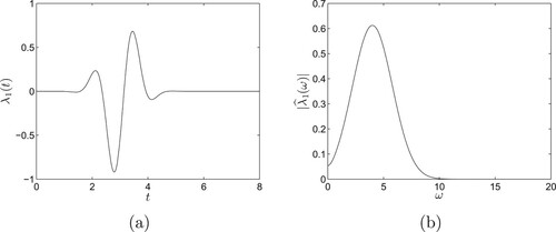
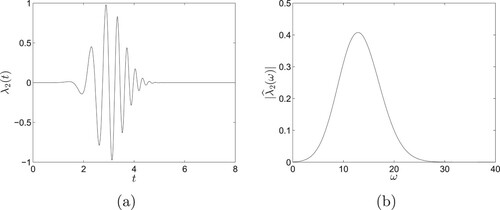
In the first experiment, the influence of the time shift μ is shown. The signal function is chosen as ${\lambda }_1(t)=\sin (4t){\mathrm{e}}^{-1.6(t-3{)}^2}.$The function ${\lambda }_1(t)$ and its Fourier spectrum are shown in Figure 1.

Figure 1. (a) The pulse function ${\lambda }_1(t)=\sin (4t){\mathrm{e}}^{-1.6(t-3{)}^2}$. (b) The Fourier spectrum $|{\hat{\lambda }}_1(\omega )|$.

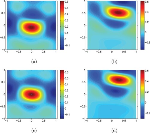
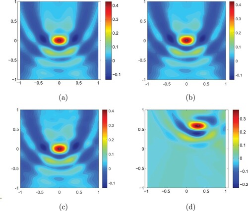
The scatterers are chosen as spherical scatterers centred at $(0,0)$ and $(0.3,0.6)$, respectively. The time shifts are chosen as $\mu =0$ (no time shift) and $\mu =0.12,$ respectively for the two cases. The reconstructions can be seen in Figure 2. As is shown in the figure, with the time shift $\mu =0.12$, the reconstructions of the spherical scatterers are more accurate. The choice of μ mainly depends on the signal function $\lambda (t)$ and is independent of the location of the scatterer.

Figure 2. (a) The reconstruction of the spherical scatterer centred at $(0,0)$, $\delta =1\mathrm{\%}$, $\mu =0$. (b) The reconstruction of the spherical scatterer centred at $(0.3,0.6)$, $\delta =1\mathrm{\%}$, $\mu =0$. (c) The reconstruction of the spherical scatterer centred at $(0,0)$, $\delta =1\mathrm{\%}$, $\mu =0.12$. (d) The reconstruction of the spherical scatterer centred at $(0.3,0.6)$, $\delta =1\mathrm{\%}$, $\mu =0.12$.

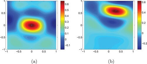
Moreover, for the spherical scatterer centred at $(0.3,0.6)$, we investigate the scattered data $u(x_i,t_k)$ given by the forward solver and the approximate solution $U(x_i,t_k;y_0)$. The wave data are shown in Figure 3, in which $t_k\in [0,15]$ and $x_i=3(\cos {\theta }_i,\sin {\theta }_i)$ for ${\theta }_i\in [0,2\pi )$. As shown in the figure, the intensity of the scattered data $u(x_i,t_k)$ greatly depends on θ while the approximate solution does not. However, the proposed method is feasible since the overall structures of the fields are similar.

Figure 3. (a) The scattered data $u(x_i,t_k)$ given by the forward solver. (b) The scattered data $U(x_i,t_k;y_0)$ given by the approximate solution.

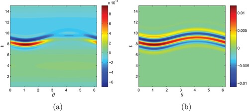
Remark 4.1

Since the forward solver depends on the forward and inverse Fourier transforms, part of the calculation error is reflected in the frequency domain data. Thus the frequency of the scattered data $u(x_i,t_k)$ is slightly different from that of the incident field.

Example 4.2

In this example, the scatterers are chosen as kite-shaped point-like scatterers centred at $(0,0)$ and $(0.3,0.6)$. The time shift is chosen as $\mu =0.12$. The reconstructions can be seen in Figure 4. As shown in the figure, the algorithm can reconstruct kite-shaped scatterers.

Figure 4. (a) The reconstruction of the kite-shaped scatterer centred at $(0,0)$, $\delta =1\mathrm{\%}$, $\mu =0.12$. (b) The reconstruction of the kite-shaped scatterer centred at $(0.3,0.6)$, $\delta =1\mathrm{\%}$, $\mu =0.12$.

Example 4.3

As shown in Figures 2 and 4, the contour lines are sparse near the local maximum point. In this example, we give an optimization with the choice of a new signal function.

Consider the artificial signal function ${\lambda }_2(t)=\sin (t^{2.5}){\mathrm{e}}^{-1.6(t-3{)}^2}.$The signal function ${\lambda }_2(t)$ and its Fourier spectrum are shown in Figure 5. Clearly, the spectrum of the signal function ${\lambda }_2(t)$ is wider than that of ${\lambda }_1(t)$.

Figure 5. (a) The pulse function ${\lambda }_2(t)=\sin (t^{2.5}){\mathrm{e}}^{-1.6(t-3{)}^2}$. (b) The Fourier spectrum $|{\hat{\lambda }}_2(\omega )|$.

The scatterers are chosen as spherical scatterers centred at $(a_1,a_2)$. The time shift is chosen as $\mu =0.21$. The reconstructions with different choices of $(a_1,a_2)$ and δ can be seen in Figure 6. As shown in the figure, the contour lines are denser for the artificial signal function ${\lambda }_2(t)$, and the algorithm is robust to noise.

Figure 6. The reconstruction of the spherical scatterer centred at $(a_1,a_2)$ with the signal function ${\lambda }_2(t)$, $\mu =0.21$. (a) $(a_1,a_2)=(0,0)$, $\delta =1\mathrm{\%}$. (b) $(a_1,a_2)=(0,0)$, $\delta =5\mathrm{\%}$. (c) $(a_1,a_2)=(0,0)$, $\delta =10\mathrm{\%}$. (d)$(a_1,a_2)=(0.3,0.6)$, $\delta =1\mathrm{\%}$.

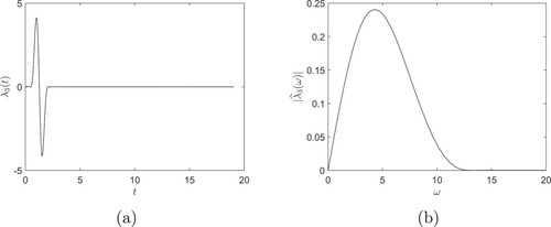
Example 4.4

We concern about the three-dimensional case in this example. The forward scattering problem is approximately calculated utilizing the k-Wave software. We choose c = 1, $N_x=50$, T = 19 and $N_t=255$ in this example. The incident wave is assumed to be emitted from the point $x_0^{\prime }=(-4,-4,-0.4)$. The scatterer is chosen as spherical scatterers centred at $(-0.6,-0.6,-0.6)$ with radius 0.1. The measurement surface is a spherical surface centred at the origin with radius 4. The measurement points and the signal function ${\lambda }_3(t)$ are automatically generated by the k-Wave software. The sketch of ${\lambda }_3(t)$ and its Fourier spectrum are shown in Figure 7.

Figure 7. (a) The pulse function ${\lambda }_3(t)$. (b) The Fourier spectrum $|{\hat{\lambda }}_3(\omega )|$.

The approximate solution (13(13) $U(x,t;y_0,\mu ):=-\frac{\lambda (t-\mu -c^{-1}|y_0-x_0|-c^{-1}|x-y_0|))}{4\pi |y_0-x_0||x-y_0|}.$(13) ) is used for the reconstruction. The time shift is chosen as $\mu =0.15$. The sampling points are chosen as $21\times 21\times 21$ equidistant points in $[-2,2]\times [-2,2]\times [-2,2]$. Random noise is added with $\delta =5\mathrm{\%}$. 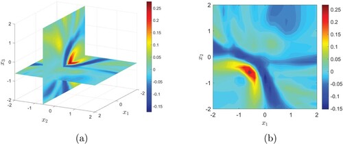The reconstructions can be seen in Figure 8 with slices through the centre of the scatterer along $x_1{x}_2$-plane and $x_1{x}_3$-plane.

Figure 8. The reconstruction of the spherical scatterer centred at $(-0.6,-0.6,-0.6)$. (a) The reconstruction of the scatterer, $\mu =0.15$, $\delta =5\mathrm{\%}$. (b) The slice through the centre of the scatterer along $x_1{x}_2$-plane.

5. Conclusion

In this paper, approximate solutions based on Green's function are provided, and a simple sampling method to reconstruct the location of a point-like scatterer is proposed. The algorithm is simple to compute, and numerical experiments are provided to show the effectiveness of the proposed method.

Acknowledgments

The work of Bo Chen was supported by the National Natural Science Foundation of China (NSFC) [grant number 11671170] and the Scientific Research Foundation of Civil Aviation University of China [grant number 2017QD04S]. The work of Yao Sun was supported by the NSFC [grant number 11501566].

Disclosure statement

No potential conflict of interest was reported by the author(s).

Additional information

Funding

The work of Bo Chen was supported by the National Natural Science Foundation of China (NSFC) [grant number 11671170] and the Scientific Research Foundation of Civil Aviation University of China [grant number 2017QD04S]. The work of Yao Sun was supported by the NSFC [grant number 11501566].

References

- Colton D, Kress R. Inverse acoustic and electromagnetic scattering theory. 3rd ed. Berlin: Springer; 2013.
- Sayas FJ. Retarded potentials and time domain boundary integral equations: a road-map. Switzerland: Springer; 2016. (Springer Series in Computational Mathematics).
- Colton D, Kirsch A. A simple method for solving inverse scattering problems in the resonance region. Inverse Probl. 1996;12(4):383–393.
- Guo Y, Hömberg D, Hu G, et al. A time domain sampling method for inverse acoustic scattering problems. J Comput Phys. 2016;314:647–660.
- Li J, Liu H, Zou J. Strengthened linear sampling method with a reference ball. SIAM J Sci Comput. 2009;31(6):4013–4040.
- Challa DP, Sini M. Inverse scattering by point-like scatterers in the Foldy regime. Inverse Probl. 2012;28(12):1224–1246.
- Cheney M. The linear sampling method and the MUSIC algorithm. Inverse Probl. 2001;17(4):591–595.
- Cheng J, Liu J, Nakamura G. The numerical realization of the probe method for the inverse scattering problems from the near-field data. Inverse Probl. 2005;21(3):839–855.
- Ikehata M. Reconstruction of the shape of the inclusion by boundary measurements. Commun Partial Differ Equ. 1998;23(7-8):1459–1474.
- Bao G, Hou S, Li P. Inverse scattering by a continuation method with initial guesses from a direct imaging algorithm. J Comput Phys. 2007;227(1):755–762.
- Barucq H, Faucher F, Pham H. Localization of small obstacles from back-scattered data at limited incident angles with full-waveform inversion. J Comput Phys. 2018;370:1–24.
- Hou S, Solna K, Zhao H. A direct imaging method using far-field data. Inverse Probl. 2007;23(4):1533–1546.
- Challa DP, Hu G, Sini M. Multiple scattering of electromagnetic waves by finitely many point-like obstacles. Math Models Methods Appl Sci. 2014;24(5):863–899.
- Gintides D, Sini M, Thành NT. Detection of point-like scatterers using one type of scattered elastic waves. J Comput Appl Math. 2012;236(8):2137–2145.
- Chen X. Multiple signal classification method for detecting point-like scatterers embedded in an inhomogeneous background medium. J Acoust Soc Am. 2010;127(4):2392–2397.
- Hu G, Andrea M, Mourad S. Direct and inverse acoustic scattering by a collection of extended and point-like scatterers. Multiscale Model Simul. 2014;12(3):996–1027.
- Lai J, Li M, Li P, et al. A fast direct imaging method for the inverse obstacle scattering problem with nonlinear point scatterers. Inverse Prob Imag. 2018;12(3):635–665.
- Yin T, Hu G, Xu L. Near-field imaging point-like scatterers and extended elastic solid in a fluid. Commun Comput Phys. 2016;19(5):1317–1342.
- Ha-Duong T. On retarded potential boundary integral equations and their discretisation. Topics Comput Wave Propag. 2003;31:301–336.
- Banjai L, Sauter S. Rapid solution of the wave equation in unbounded domains. SIAM J Numer Anal. 2008;47(1):227–249.
- Hackbusch W, Kress W, Sauter SA. Sparse convolution quadrature for time domain boundary integral formulations of the wave equation. IMA J Numer Anal. 2009;29(1):15–20.
- Laliena AR, Sayas FJ. Theoretical aspects of the application of convolution quadrature to scattering of acoustic waves. Numer Math. 2009;112(4):637–678.
- Chen B, Guo Y, Ma F, et al. Numerical schemes to reconstruct three dimensional time dependent point sources of acoustic waves. Inverse Probl. 2020;36(7):075009.
- Chen B, Ma F, Guo Y. Time domain scattering and inverse scattering problems in a locally perturbed half-plane. Appl Anal. 2017;96(8):1303–1325.
- Chen Q, Haddar H, Lechleiter A, et al. A sampling method for inverse scattering in the time domain. Inverse Probl. 2010;26(8):85001–85017.
- Guo Y, Monk P, Colton D. Toward a time domain approach to the linear sampling method. Inverse Probl. 2013;29(9):095016.
- Chen B, Ma F, Guo Y. Acoustic scattering from open cavities in the time domain. Electron J Differ Equ. 2019;2019(131):1–14.
- Colton D, Kress R. Integral equation methods in scattering theory. New York (NY): John Wiley; 1983.
- Sun Y. Indirect boundary integral equation method for the Cauchy problem of the Laplace equation. J Sci Comput. 2017;71(2):469–498.
- Barucq H, Diaz J, Mattesi V, et al. Asymptotic behavior of acoustic waves scattered by very small obstacles. ESAIM: Math Model Numer Anal. doi:https://doi.org/10.1051/m2an/2020047
- Treeby BE, Cox BT. K-Wave: MATLAB toolbox for the simulation and reconstruction of photoacoustic wave fields. J Biomed Opt. 2010;15(2):021314.