Bayesian estimation and uncertainty quantification in models of urea hydrolysis by E. coli biofilms

ABSTRACT

Urea-hydrolysing biofilms are crucial to applications in medicine, engineering, and science. Quantitative information about ureolysis rates in biofilms is required to model these applications. We formulate a novel model of urea consumption in a biofilm that allows different kinetics, for example either first order or Michaelis–Menten. The model is fit to synthetic data to validate and compare two approaches, Bayesian and nonlinear least squares (NLS), commonly used by biofilm practitioners. The shortcomings of NLS motivate the Bayesian approach where a simple Markov Chain Monte Carlo (MCMC) sampler is applied. The model is then fit to real data of influent and effluent urea concentrations from experiments with biofilms of Escherichia coli. Results from synthetic data aid in interpreting results from real data, where first-order and Michaelis–Menten kinetic models are compared. The method shows potential for general applications requiring biofilm kinetic information.

Keywords:

• Biofilm
• modelling
• ureolysis
• uncertainty quantification
• Markov
• inverse problem
• parametrisation

2010 Mathematics Subject Classification:

• 92

1. Introduction

Microbial biofilms are almost everywhere. A deeper understanding of biofilms over the last 30 years has already transformed the way humans understand and interact with the microbial world. Microbiologists have unprecedented access to chemical, molecular and imaging technologies, and advances in mathematical modelling, that have revolutionised the study of these microbial communities. Here we focus on the mathematical and experimental modelling of microbial formation of carbonate precipitates, significant in a number of applications including industrial, medical, engineering, and agricultural contexts. In medical applications, ureolytic microorganisms can play a role in the formation of kidney stones as well as crystal encrustations on urinary tract catheters [1,2]. In engineering applications, ureolytic mineral formation has been used to protect building materials through mineral deposition [3] as well as reduce permeability in the subsurface [4]. In agricultural contexts urea is a major source of nitrogen in fertilizer that can contaminate groundwater [5] and require remediation. In each of these scenarios, biofilms are an important source of ureolytic activity.

While there are multiple ways organisms engage in biomineralisation, our interest is here confined to biomineralisation via urea hydrolysis (‘ureolysis’). Urea hydrolysis is a biochemical mechanism whereby microorganisms break down urea triggering an increase in pH, which can in turn trigger precipitation of carbonate and other minerals. At circumneutral pH levels urea hydrolysis can be written as $\mathrm{C}\mathrm{O}(\mathrm{N}{\mathrm{H}}_2{)}_2+2{\mathrm{H}}_2\mathrm{O}+{\mathrm{H}}^{+}\to 2\mathrm{N}{\mathrm{H}}_4^{+}+\mathrm{H}\mathrm{C}{\mathrm{O}}_3^{-}.$Here two ammonium ions and one bicarbonate ion are formed by the hydrolysis of each urea molecule. One proton is consumed in the reaction, which causes an increase in pH. This pH increase results in the formation of carbonate ions. This in turn can lead to the precipitation of calcium carbonate when calcium ions are introduced [6].

Quantitative information about ureolysis rates in biofilms is critical to understanding and applying ureolytic systems. While planktonic cultures have been well studied, much less is known about ureolysis rates in biofilms [7]. There have been studies of volume averaged rates in porous media [8,9] as well as in immobilised enzymes [10,11]. However, these studies have tended to concentrate on precipitation rates rather than ureolysis kinetics. Here we focus on ureolysis kinetics by biofilms in a tube reactor under continuous flow. We parameterise a novel, low dimensional pore flow model for the microbial formation of carbonate precipitates by biofilms via urea hydrolysis using experimental observations. We then formulate an inverse problem to estimate the kinetics parameters of this model from data.

Inverse problems arise in a variety of scientific fields whenever mathematical models are used to explain or extend observations. In an inverse problem, the goal is to estimate model parameters; in many situations these parameters are difficult to measure directly. Geology and earth sciences, including hydrology, have long used inverse methods (see for instance [12,13]). Inverse methods, including Bayesian statistical frameworks, have also been used in fields such as structural mechanics and heat conduction [14,15]. However, we are aware of only a handful of previous attempts to combine inverse methods and biofilm models [16–20]. Following common practice, the inverse problem we formulate is solved first using nonlinear least squares (NLS) [7,21], and then, when NLS proves insufficient, using a Bayesian approach with a simple Markov Chain Monte Carlo (MCMC) method. We compare the NLS and the Bayesian approaches for estimating parameters in our kinetics model. We apply these methods to several synthetic data sets to verify our methods before applying the methods to real data from experiments of Escherichia coli biofilms. We provide details of the implementations regarding assessing convergence and auto correlation of the algorithm's outputs.

The paper is structured as follows. In Section 2 we describe the tube reactor model and the associated inverse problem. We then briefly summarise experimental measurements before discussing the creation of synthetic data used to test the inverse methods and the model implementation. In Section 3 we discuss parameter estimation using the synthetic data and then the experimental data. In the final section we suggest four important lessons experimenters should take from this work.

2. Materials and methods

In this section we begin by describing our model. This requires a description of urea transport in the tube (Section  2.1.1), in the biofilm (Section  2.1.2), and the unification of the two (Section  2.1.3). We next describe the three inverse problems we consider in Section 2.2. These consist of both nonlinear least squares (Section  2.2.1) and a generalised Bayesian approach (Section  2.2.2). We close this section with descriptions of synthetic and experimental data.

2.1. The forward problem

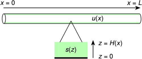
The process of calculating causal factors (here model kinetic parameters) from a set of observations (measured urea concentration) is called an inverse problem. To specify an inverse problem requires a mathematical model of the system under study, which can predict the value of the observations given a complete knowledge of the inputs. This prediction is called the ‘forward’ or ‘direct’ problem [22]. Here we develop the forward problem by unifying two one-dimensional models, one which models the axial flow of urea down a tube and one which models the consumption of urea in the tube-lining biofilm. A model schematic is shown in Figure 1.

Figure 1. Model cartoon. The unified model consists of two linked one dimensional models. The first, illustrated at the top of the figure, is a biofilm-lined tube extending in the x-dimensions, models the concentration of urea in the fluid flowing axially through tube reactor (the biofilm is represented in green). The second, represented by the expanded view at the bottom of the figure, models the concentration of urea in the wall-mounted biofilm in the radial direction, which is perpendicular to the flow. This is the z-dimension.

2.1.1. Tube reactor model

In the axial direction we assume conditions are uniform radially, allowing us to model the reactor as a long, thin tube of constant radius r extending along the x-axis. Fluid containing a specified concentration of urea enters the reactor at x = 0, travels through the tube with fixed velocity v, and exits at x = L. In addition to advective transport, we assume that urea can diffuse throughout the reactor with diffusivity D. The urea in the bulk fluid enters the reactor at x = 0 with velocity v at concentration $u^0$. Thus, if the system has reached steady state, the urea concentration at location x, denoted $u\left(x\right)$, with a flux-balanced inflow boundary condition and a no-flux outflow lower boundary condition, is given by (1a) $\begin{array}{rl}0& =D\frac{{\mathrm{d}}^{2}u}{\mathrm{d}{x}^2}-v\frac{\mathrm{d}u}{\mathrm{d}x}-\delta R\left(u\right),\end{array}$(1a) (1b) $\begin{array}{rl}v{u}^0& =-D\frac{\mathrm{d}u}{\mathrm{d}x}{|}_0+vu\left(0\right),\frac{\mathrm{d}u}{\mathrm{d}x}{|}_L=0.\end{array}$(1b) Here δ is the ratio of the circumference of the tube to its cross-sectional area, and R is the urea utilisation rate function, which depends on u (and thus x). This term provides the link between urea in the flow and urea usage by the biofilm attached to the tube walls. Note that urea concentration u is assumed to be a function of x. Hence $u\left(0\right)$ denotes the concentration of urea at x = 0 and is not equal to $u^0$ due to diffusion and advection as seen in (1b(1b) $\begin{array}{rl}v{u}^0& =-D\frac{\mathrm{d}u}{\mathrm{d}x}{|}_0+vu\left(0\right),\frac{\mathrm{d}u}{\mathrm{d}x}{|}_L=0.\end{array}$(1b) ).

2.1.2. Biofilm model

The 1D biofilm model makes three basic assumptions, namely, that properties of the biofilm change only in the direction perpendicular to the tube wall, that the biofilm may be treated as a continuum, and that the bulk fluid does not advect through the biofilm. If we further assume that the biofilm is at a steady state and has a static physical profile, then the concentration of a substrate s in the biofilm depends only on the distance z from the wall. The concentration of urea at the top of the biofilm (z = H) matches that in the bulk fluid, $s^0$, and we assume that the wall is impermeable. The model is then (2a) $\begin{array}{rl}& -D\frac{{\mathrm{d}}^{2}s}{\mathrm{d}{z}^2}=r(s;\theta ),\end{array}$(2a) (2b) $\begin{array}{rl}& s\left(H\right)=s^0,\frac{\mathrm{d}s}{\mathrm{d}z}{|}_{z=0}=0.\end{array}$(2b) Note that here we use the same diffusion coefficient, D, as in the bulk fluid, though in general diffusion inside and outside of the biofilm may vary by a small scale factor [23].

The difficulty in solving this model depends entirely on the reaction function $r(s;\theta )$ for urea inside the biofilm, which in turn depends on the kinetic model used. We use θ to represent the (possibly unknown) kinetic parameter(s). Regardless of details regarding the formulation of $r(s;\theta )$, we are interested in the flux of substrate into the top of the biofilm from the bulk fluid. This is described by the unknown flux (3) $Q_H=-D\frac{\mathrm{d}s}{\mathrm{d}z}{|}_{(z=H;\theta )},$(3) a quantity we will use to link the 1D biofilm and 1D tube models.

2.1.3. Unified model

The key to combining these models is the realisation that the utilisation rate $R\left(u\right)$ from the tube reactor model (cf. (1a(1a) $\begin{array}{rl}0& =D\frac{{\mathrm{d}}^{2}u}{\mathrm{d}{x}^2}-v\frac{\mathrm{d}u}{\mathrm{d}x}-\delta R\left(u\right),\end{array}$(1a) )) is linked to the flux of substrate into the biofilm shown in (3(3) $Q_H=-D\frac{\mathrm{d}s}{\mathrm{d}z}{|}_{(z=H;\theta )},$(3) ). As substrate is consumed in the biofilm, local concentration in the biofilm is diminished, driving a Fickian flux of material from the tube reactor into the biofilm. To derive the unified model we equate $R\left(u\right)$ in (1a(1a) $\begin{array}{rl}0& =D\frac{{\mathrm{d}}^{2}u}{\mathrm{d}{x}^2}-v\frac{\mathrm{d}u}{\mathrm{d}x}-\delta R\left(u\right),\end{array}$(1a) ) with $Q_H\left(S\right)$ in (3(3) $Q_H=-D\frac{\mathrm{d}s}{\mathrm{d}z}{|}_{(z=H;\theta )},$(3) ). We then nondimensionalise using $S=\frac{s}{s^0}$ and $Z=\frac{z}{H}$ in the z dimension, and $X=\frac{x}{L}$ and $U=\frac{u}{u^0}$ in the x dimension. This change of variables means that Z = 0 is the bottom of the biofilm, and Z = 1 is the surface. Similarly, X = 0 is the tube entrance and X = 1 the exit. We further note that $s^0=u\left(x\right)$, and define nondimensional parameters $\mathrm{P}\mathrm{e}=\frac{vL}{D}$, a Péclet number relating advective transport to diffusive transport, and $\text{β}\left(X\right)=\delta L\frac{D_e}{vH\left(X\right)}$, a product of nondimensional numbers which is large under conditions where urea utilisation is high and small under conditions where urea utilisation is small. While any suitable reference concentration may be used for $u^0$, we use the influent concentration of urea. The unified model may then be written as (4a) $\begin{array}{rl}0& =\frac{1}{\mathrm{P}\mathrm{e}}{U}^{″}-U^{\prime }-\text{β}(X;H(X\left)\right)U\frac{\mathrm{d}S}{\mathrm{d}Z}(Z=1;\theta ),\end{array}$(4a) (4b) $\begin{array}{rl}1& =-\frac{1}{\mathrm{P}\mathrm{e}}{U}^{\prime }\left(0\right)+U\left(0\right),U^{\prime }\left(1\right)=0,\end{array}$(4b) where the prime indications differentiation with respect to X and $\frac{\mathrm{d}S}{\mathrm{d}Z}(Z=1;\theta )$ implicitly depends on some set of parameters θ.

Experimental data, summarised in Table 1, shows that the Péclet number for the tube reactors is on the order of ${10}^4$, meaning that the $1/\mathrm{P}\mathrm{e}$ terms in (4(4a) $\begin{array}{rl}0& =\frac{1}{\mathrm{P}\mathrm{e}}{U}^{″}-U^{\prime }-\text{β}(X;H(X\left)\right)U\frac{\mathrm{d}S}{\mathrm{d}Z}(Z=1;\theta ),\end{array}$(4a) ) are very small. This means that diffusion is far less important to the transport of urea than advection. Omitting these small terms, the unified model can be simplified to $\begin{array}{rl}& U^{\prime }=\text{β}(X;H(X\left)\right)U\left(X\right)\frac{\mathrm{d}S}{\mathrm{d}Z}(Z=1;\theta ),\\ & U\left(0\right)=1.\end{array}$The removal of the second-order term reduces the order of the unified model, which means that both boundary conditions in (4b(4b) $\begin{array}{rl}1& =-\frac{1}{\mathrm{P}\mathrm{e}}{U}^{\prime }\left(0\right)+U\left(0\right),U^{\prime }\left(1\right)=0,\end{array}$(4b) ) cannot be imposed. We chose to retain the influent boundary condition because it contains model data in the form of $U\left(0\right)$.

Table 1. A summary of parameter values used in the unified tube reactor model.

Name:	value:	units:	description:	source:
r	0.8	mm	inner radius of tube reactor	measurement
δ	2.5	1/mm	ratio of circumf. to area	calculated
L	1000	mm	length of reactor	measurement
D	4.932	mm^2/hr	diffusivity of urea in water	[24]
Q	1000	mm^3/hr	fluid flux through reactor	measurement
v	497.4	mm/hr	average fluid velocity	calculated as $Q/\pi r^2$
$\mathrm{P}\mathrm{e}$	10084	1	Péclet number	calculated as vL/D
$u^0$	0.5, 5, 10, 15	g/L	influent urea concentration	measurement
$H\left(X\right)$	0–0.35	mm	biofilm thickness	measurement

It is common for mathematicians to nondimensionalise a model as in the previous equation, which eases computations and interpretation. Unfortunately, this nondimensional form makes it challenging to see the dependence on other inputs from data such as the urea influent into the tube, $u^0$, which is crucial for working with the inverse problem that we describe later. Hence, we rewrite the model, in a nonstandard form, as (5a) $\begin{array}{rl}& \frac{\mathrm{d}u}{\mathrm{d}X}=\text{β}(X;H(X\left)\right)u\left(X\right)\frac{\mathrm{d}S}{\mathrm{d}Z}(Z=1;\theta ),\end{array}$(5a) (5b) $\begin{array}{rl}& u\left(0\right)=u^0.\end{array}$(5b)

The model given by (5(5a) $\begin{array}{rl}& \frac{\mathrm{d}u}{\mathrm{d}X}=\text{β}(X;H(X\left)\right)u\left(X\right)\frac{\mathrm{d}S}{\mathrm{d}Z}(Z=1;\theta ),\end{array}$(5a) ) describes how much urea $u\left(x\right)$ is at location x in the biofilm-laden tube given a specification of the unknown kinetic parameters θ, the influent urea concentration $u^0$, and a height profile H of the biofilm in the tube. In real experiments, it is only practical to measure urea concentration at the tube's effluent $u_L=u(x=L)$, while the influent concentration $u^0=u(x=0)$ into the tube is controlled by the experimenter and is assumed known. Because the urea concentration inside the tube ($u\left(x\right)$ for $0<x<L)$ is not observable in our experiments, we focus on ${\hat{u}}_L=\hat{u}(x=L)$, an estimate of the effluent urea concentration $u(x=L)$. We graphically compare these measured and modelled quantities for real experimental data in Section 3.2.

The solution of the system (5(5a) $\begin{array}{rl}& \frac{\mathrm{d}u}{\mathrm{d}X}=\text{β}(X;H(X\left)\right)u\left(X\right)\frac{\mathrm{d}S}{\mathrm{d}Z}(Z=1;\theta ),\end{array}$(5a) ) that relates the parameters θ to the output ${\hat{u}}_L$ is the ‘forward map’ or ‘forward problem’. We will write ${\hat{u}}_L=g(\theta ;u^0,H)$ where $g(\cdot )$ indicates the forward map as a function of θ, with dependencies on $u^0$ and H that are set from experimental data. Note that the evaluation of the forward problem (i.e. solving (5(5a) $\begin{array}{rl}& \frac{\mathrm{d}u}{\mathrm{d}X}=\text{β}(X;H(X\left)\right)u\left(X\right)\frac{\mathrm{d}S}{\mathrm{d}Z}(Z=1;\theta ),\end{array}$(5a) )) requires solving the differential equation shown in (2(2a) $\begin{array}{rl}& -D\frac{{\mathrm{d}}^{2}s}{\mathrm{d}{z}^2}=r(s;\theta ),\end{array}$(2a) ) at each mesh-point to compute $\frac{\mathrm{d}S}{\mathrm{d}Z}(Z=1;\theta )$. This can be a time-consuming calculation (see Section 2.5).

The unified model (5(5a) $\begin{array}{rl}& \frac{\mathrm{d}u}{\mathrm{d}X}=\text{β}(X;H(X\left)\right)u\left(X\right)\frac{\mathrm{d}S}{\mathrm{d}Z}(Z=1;\theta ),\end{array}$(5a) ) is a general framework for generating different forward problems that describe how the biofilm breaks down urea via the function $r(s;\theta )$ in (2a(2a) $\begin{array}{rl}& -D\frac{{\mathrm{d}}^{2}s}{\mathrm{d}{z}^2}=r(s;\theta ),\end{array}$(2a) ); $r(s;\theta )$ affects the unified model through the $\frac{\mathrm{d}S}{\mathrm{d}Z}(Z=1;\theta )$ term in (5a(5a) $\begin{array}{rl}& \frac{\mathrm{d}u}{\mathrm{d}X}=\text{β}(X;H(X\left)\right)u\left(X\right)\frac{\mathrm{d}S}{\mathrm{d}Z}(Z=1;\theta ),\end{array}$(5a) ). A given forward problem has unknown parameters θ that need to be estimated from data. In general, θ can be either a scalar or vector depending on the choice of kinetics, i.e. choice of $r(s;\theta )$. We consider 2 forward problems:

(FP1)	To describe first-order kinetics, the forward model $g(\theta ;u^0,H)$ that describes (5(5a) $\begin{array}{rl}& \frac{\mathrm{d}u}{\mathrm{d}X}=\text{β}(X;H(X\left)\right)u\left(X\right)\frac{\mathrm{d}S}{\mathrm{d}Z}(Z=1;\theta ),\end{array}$(5a) ) utilises $r(s;\theta )=k_{1}s$, so there is a single unknown parameter, $\theta =k_1$.
(FP2)	For Michaelis–Menten kinetics, the forward model $g(\theta ;u^0,H)$ that describes (5(5a) $\begin{array}{rl}& \frac{\mathrm{d}u}{\mathrm{d}X}=\text{β}(X;H(X\left)\right)u\left(X\right)\frac{\mathrm{d}S}{\mathrm{d}Z}(Z=1;\theta ),\end{array}$(5a) ) utilises $r(s;\theta )=r_{0}s/(k_m+s)$, so there are two unknown parameters, $\theta =(r_0,k_m)$.

The forward problems (FP1) and (FP2) presume that the kinetic properties of the microbes in question, θ, are constant with respect to urea concentration and are invariant with respect to model environmental conditions. Relaxing this assumption would increase the complexity of the model and increase the number of parameters.

2.1.4. Error model

We know that the model ${\hat{u}}_L=g(\theta ;u^0,H)$ in either (FP1) or (FP2) will not perfectly predict the real experimental effluent urea data ${\mathbf{u}}_L$, i.e. there will be error. We assume that the errors are independent and identically distributed (iid) [25, p. 155], which means that effluent concentrations from different individual tube reactors do not affect each other, and that the same parameters θ govern the kinetics in all the tubes used in experiments. We also assume that the errors are normally distributed with standard deviation σ, a common assumption for many processes ([26, p.88, 117], [27, p.1196–1197]) due to its simplicity. Given this assumption, the process that generates experimental data can be written as ${\mathbf{u}}_L=\mathbf{g}(\theta ;u^0,H)+ϵ,$where $ϵ\sim N_n(0,{\sigma }^{2}I)$. Here $N_n$ is the multivariate normal (MVN) distribution of dimension n, where n is the length of ${\mathbf{u}}_L$ and corresponds to the number of observed effluent values. It follows that ${\mathbf{u}}_L$, given θ, is normally distributed with mean $\mathbf{g}(\theta ;u^0,H)$ and standard deviation σ [25, p. 155]. That is, (6) ${\mathbf{u}}_L\mid \theta ,{\sigma }^2\sim N_n\left(\mathbf{g}\right(\theta ;u^0,H),{\sigma }^{2}I),$(6) where $N_n\left(\mathbf{g}\right(\theta ;u^0,H),{\sigma }^{2}I)$ is the likelihood. Using $P(\cdot )$ to represent probability density functions, we can write the MVN likelihood explicitly as (7) $P(u_L\mid \theta ,{\sigma }^2)=\sqrt{\frac{1}{(2\pi {)}^n{\sigma }^2}}\exp \left(-\frac{1}{2{\sigma }^2}\parallel {\mathbf{u}}_L-\mathbf{g}(\theta ;u^0,H){\parallel }_2^2\right).$(7)

2.2. The inverse problem

The forward problems (FP1) and (FP2) describe how much urea, $u_L$, exits a biofilm-laden tube given values of the parameters θ. The inverse problem is to estimate the parameters of interest, θ, given observed urea concentrations $u_L$ from a biofilm-laden tube. When collecting new experimental data, we must also estimate the standard deviation of the error, σ.

We consider 3 inverse problems:

(IP1)	Given data and the forward model (FP2) that describes Michaelis–Menten kinetics, estimate two parameters, $\theta =(r_0,k_m)$. The standard deviation σ is assumed to be known and is set at a fixed value.
(IP2)	Given data and the forward model (FP1) that describes first-order kinetics, estimate $\theta =k_1$ and σ.
(IP3)	Given data and the forward model (FP2) that describes Michaelis–Menten kinetics, estimate $\theta =(r_0,k_m)$ and σ.

Solving the problems (IP2) and (IP3) provides an estimate of the standard deviation σ of the error. Note that this estimate for σ can be useful for estimating how many tube reactors to include in a future experiment to attain a desired level of precision.

Using the synthetic and real experimental data that we describe in the rest of this section, we apply NLS and a Bayesian approach to solve these inverse problems given the same data sets.

2.2.1. Nonlinear least squares

The simplest and most naive approach to solving an inverse problem is to formulate a cost function comparing the difference between model output and experimental values and then seek to minimise this function with respect to model inputs θ. When the cost function is $\parallel \cdot {\parallel }_2^2$, then this is a nonlinear least squares (NLS) formulation. Denote the vector of experimentally measured effluent concentrations by ${\mathbf{u}}_L$. The cost function $c\left(\theta \right)$ is (8) $c\left(\theta \right)=\parallel ({\mathbf{u}}_L-{\hat{\mathbf{u}}}_L){\parallel }_2^2.$(8) The n-vector ${\hat{\mathbf{u}}}_L=\mathbf{g}(\theta ;u^0,H)$ predicts effluent concentrations from n biofilm-laden tube reactors given values for the parameters θ, the influent $u^0$ and biofilm height profile H; $g(\cdot )$ indicates one of the forward maps (FP1) or (FP2). Using the NLS approach we seek an optimal value of θ, denoted ${\theta }_{\mathrm{n}\mathrm{l}\mathrm{s}}$, such that ${\theta }_{\mathrm{n}\mathrm{l}\mathrm{s}}=\mathrm{a}\mathrm{r}\mathrm{g}\mathrm{m}\mathrm{i}\mathrm{n}c\left(\theta \right)$. As we shall see, this approach is uninformative for some parameter sets, though (8(8) $c\left(\theta \right)=\parallel ({\mathbf{u}}_L-{\hat{\mathbf{u}}}_L){\parallel }_2^2.$(8) ) remains an important component for more advanced methods. Another drawback to NLS is that resulting confidence intervals are computed by adding and subtracting a calculated margin of error from ${\theta }_{\mathrm{n}\mathrm{l}\mathrm{s}}$ (under the assumption that ${\theta }_{\mathrm{n}\mathrm{l}\mathrm{s}}$ is normally distributed). This means that confidence intervals formed via NLS are necessarily symmetric even when the underlying distribution of ${\theta }_{\mathrm{n}\mathrm{l}\mathrm{s}}$ is skewed.

2.2.2. A Bayesian approach

A more sophisticated approach for solving a nonlinear inverse problem that addresses the deficiencies of NLS involves Bayesian inference.

Given the likelihood (7(7) $P(u_L\mid \theta ,{\sigma }^2)=\sqrt{\frac{1}{(2\pi {)}^n{\sigma }^2}}\exp \left(-\frac{1}{2{\sigma }^2}\parallel {\mathbf{u}}_L-\mathbf{g}(\theta ;u^0,H){\parallel }_2^2\right).$(7) ) and a value of θ, we can calculate the probability that an effluent urea concentration falls within a particular range. But this is the opposite of what we want when working with real data because in that case we do not know the value of θ. Rather, we need the posterior distribution $P(\theta \mid u_L)$, which gives us the probability density of seeing particular values of θ given the observed data. NLS and the resulting confidence intervals work well when this posterior is approximately normal (and hence symmetric), but this need not be the case. The Bayesian approach generates an approximation to the posterior distribution for θ, from which some statistic can be calculated to estimate θ with a single value, such as the median, or the mode referred to as the ‘maximum a posteriori’ or MAP. An interval estimate for θ is provided by calculating a probability interval or ‘credible interval’ directly from the posterior. It is important to note that the terminology ‘credible interval’ specifies a Bayesian interval estimate from the posterior, whereas a confidence interval from NLS is calculated by assuming that ${\theta }_{\mathrm{n}\mathrm{l}\mathrm{s}}$ is normally distributed.

Bayes' Theorem is the key to calculating the posterior because it relates the known likelihood to the unknown posterior distribution. To compute the posterior up to a normalising constant we multiply the likelihood distribution by the prior distribution, $P_0\left(\theta \right)$. Explicitly, by Bayes' Theorem [25, p. 156] (9) $P(\theta \mid u_L,{\sigma }^2)=\frac{P(u_L\mid \theta ,{\sigma }^2)P_0\left(\theta \right)}{P\left(u_L\right)},$(9) in the case that we consider ${\sigma }^2$ known. If we allow that ${\sigma }^2$ is unknown then it must be estimated using the Bayesian approach and the posterior is (10) $P(\theta ,{\sigma }^2\mid u_L)\propto P(u_L\mid \theta ,{\sigma }^2)P(\theta ,{\sigma }^2)=P(u_L\mid \theta ,{\sigma }^2)P_0\left(\theta \right)P_0\left({\sigma }^2\right).$(10) Here we write the joint prior $P_0(\theta ,{\sigma }^2)$ as a product of the marginal priors, $P_0\left(\theta \right)P_0\left({\sigma }^2\right)$, because we assume independence of kinetic parameters and experimental precision.

The same prior distribution $P_0\left(\theta \right)$ is used for all 3 inverse problems (IP1)–(IP3) that we consider; and the same prior $P_0\left({\sigma }^2\right)$ is used for both (IP2) and (IP3). The prior distribution for θ, $P_0\left(\theta \right)$, contains whatever knowledge we have regarding θ prior to observing the data (e.g. see [28, p. 43]; [26, p. 61]; [29, p. 40]; [30, p. 297, 463, 473]; [31, p. 224]; [32, p. 115]; [33, p. 92]; and [34, p. 797]. Here we impose upper and lower bounds for the parameters of interest θ, and we assume that the prior probability is uniformly distributed between these bounds.

We use an inverse-${\chi }^2$-distribution for ${\sigma }^2$ [35, p. 75] (11) $P_0({\sigma }^2\mid \nu ,{\hat{\sigma }}^2)=\left\{\begin{array}{ll}\frac{2^{-\nu /2}}{\mathrm{\Gamma }\left(\nu /2\right)}{\left({\hat{\sigma }}^2\nu /{\sigma }^2\right)}^{\nu /2-1}{e}^{-{\hat{\sigma }}^2\nu /\left(2{\sigma }^2\right)}& \mathrm{i}\mathrm{f}{\sigma }^2>0,\\ 0& \mathrm{o}\mathrm{t}\mathrm{h}\mathrm{e}\mathrm{r}\mathrm{w}\mathrm{i}\mathrm{s}\mathrm{e},\end{array}\right.$(11) where n is the number of sampled effluent concentrations and $\nu =n-1$. Evaluating this prior requires an estimate ${\hat{\sigma }}^2$ (see section 2.5). There are other more standard prior models we could have used, for example the so-called Jeffrey's prior ([35, p. 62]; [25, p. 164]) or an inverse-gamma (e.g. see [30, p. 335]; [36], [25, p. 163]) for which (11(11) $P_0({\sigma }^2\mid \nu ,{\hat{\sigma }}^2)=\left\{\begin{array}{ll}\frac{2^{-\nu /2}}{\mathrm{\Gamma }\left(\nu /2\right)}{\left({\hat{\sigma }}^2\nu /{\sigma }^2\right)}^{\nu /2-1}{e}^{-{\hat{\sigma }}^2\nu /\left(2{\sigma }^2\right)}& \mathrm{i}\mathrm{f}{\sigma }^2>0,\\ 0& \mathrm{o}\mathrm{t}\mathrm{h}\mathrm{e}\mathrm{r}\mathrm{w}\mathrm{i}\mathrm{s}\mathrm{e},\end{array}\right.$(11) ) is a special case.

2.2.3. The Bayesian solution

When solving the inverse problem (IP1), we suppose that the error standard deviation σ is known, and that $\theta =(r_0,k_m)$. Let $I_{r_0}=[r_0^{\mathrm{m}\mathrm{i}\mathrm{n}},r_0^{\mathrm{m}\mathrm{a}\mathrm{x}}]$ and $I_{k_m}=[k_m^{\mathrm{m}\mathrm{i}\mathrm{n}},k_m^{\mathrm{m}\mathrm{a}\mathrm{x}}]$ denote the support for $r_0$ and $k_m$, respectively, so that $P_0\left(\theta \right)$ is a uniform distribution over $I_{r_0}\times I_{k_m}$. Then, the posterior from (9(9) $P(\theta \mid u_L,{\sigma }^2)=\frac{P(u_L\mid \theta ,{\sigma }^2)P_0\left(\theta \right)}{P\left(u_L\right)},$(9) ) is (12) $P(\theta \mid u_L,{\sigma }^2)=\left\{\begin{array}{ll}\frac{P(u_L\mid \theta ,{\sigma }^2)P_0\left(\theta \right)}{P\left(u_L\right)},& \mathrm{i}\mathrm{f}\theta \in I_{r_0}\times I_{k_m},\\ 0& \mathrm{o}\mathrm{t}\mathrm{h}\mathrm{e}\mathrm{r}\mathrm{w}\mathrm{i}\mathrm{s}\mathrm{e}.\end{array}\right.$(12) With only two dimensions and finite support, it follows that we can discretise $I_{r_0}\times I_{k_m}$ into an $m\times m$ grid and, after evaluating the posterior (and hence the forward problem) at every grid point, simply approximate the integral in the denominator of (12(12) $P(\theta \mid u_L,{\sigma }^2)=\left\{\begin{array}{ll}\frac{P(u_L\mid \theta ,{\sigma }^2)P_0\left(\theta \right)}{P\left(u_L\right)},& \mathrm{i}\mathrm{f}\theta \in I_{r_0}\times I_{k_m},\\ 0& \mathrm{o}\mathrm{t}\mathrm{h}\mathrm{e}\mathrm{r}\mathrm{w}\mathrm{i}\mathrm{s}\mathrm{e}.\end{array}\right.$(12) ) using a numeric scheme such as the trapezoidal method. In the Results, we used m = 100. Because $P(u_L|\theta ,{\sigma }^2)\propto e^{-1/2{\sigma }^{2}c\left(\theta \right)}$, this direct calculation of the posterior requires computing the cost function (8(8) $c\left(\theta \right)=\parallel ({\mathbf{u}}_L-{\hat{\mathbf{u}}}_L){\parallel }_2^2.$(8) ) ${10}^4$ times, which is computationally expensive but acceptable. Solving (IP2) can also be solved over a grid, but now the grid is over $I_{k_1}\times I_{{\sigma }^2}$.

Solving an inverse problem with more than two parameters, such as (IP3), benefits from a more efficient approach. For (IP3), to estimate the three dimensional posterior $P(\theta ,{\sigma }^2\mid u_L)$ in (10(10) $P(\theta ,{\sigma }^2\mid u_L)\propto P(u_L\mid \theta ,{\sigma }^2)P(\theta ,{\sigma }^2)=P(u_L\mid \theta ,{\sigma }^2)P_0\left(\theta \right)P_0\left({\sigma }^2\right).$(10) ) when σ is unknown, we do not compute the posterior given by (10(10) $P(\theta ,{\sigma }^2\mid u_L)\propto P(u_L\mid \theta ,{\sigma }^2)P(\theta ,{\sigma }^2)=P(u_L\mid \theta ,{\sigma }^2)P_0\left(\theta \right)P_0\left({\sigma }^2\right).$(10) ) over the full support of the parameters, but instead draw samples from $P(\theta ,{\sigma }^2\mid u_L)$ using a Markov Chain Monte Carlo (MCMC) method. MCMC works by constructing a Markov chain of samples whose stationary distribution is the posterior density function. The samples of this chain provide a picture of the posterior density after the chain converges to the stationary distribution. Early samples in the chain are generally discarded as ‘burn-in’ because the chain may not start near the stationary distribution [35, p. 295]. More details of our simple MCMC implementation are provided in Section 2.5. One very useful consequence of using MCMC when solving (IP2) and (IP3) is that the chains for the parameters of interest (θ) give samples for the ‘marginal posterior’ for θ ($P\left(\theta |u_L\right)$) after integrating out the ‘nuisance’ parameter σ (i.e. $P\left(\theta |u_L\right)=\int P(\theta ,\sigma |u_L)d\sigma$).

There are alternatives to the Bayesian approach such as likelihood profiling [37] and bootstrapping [38]. However, neither of these methods incorporate prior knowledge about the parameters.

2.3. Real experimental measurements

The methods and materials used to collect data on biofilm growth and thickness data have been published in detail elsewhere [6]. We provide a brief summary here.

Cultures of a biofilm containing a green fluorescent protein gene (GFP) were grown in 10 cm long silicone tubes with an interior diameter of 0.8 mm to mimic biofilm growing in small pore-spaces. The microorganism was Escherichia coli MJK2 [39], which is a GFP strain selected to aid in imaging and biofilm quantification. After the tubes were inoculated, syringe pumps pushed sterile media containing urea in concentrations ranging from 0.1 g/L to 15 g/L through the tubing at a rate of 1.0 mL/hr for as little as 10 days, or for more than two months, depending on the experiment. Flow was continuous except for short periods when the syringe pumps were exchanged. Sample ports upstream allowed influent samples to be taken for analysis, while effluent samples were taken by simply disconnecting the downstream end of the tube and filling a vial.

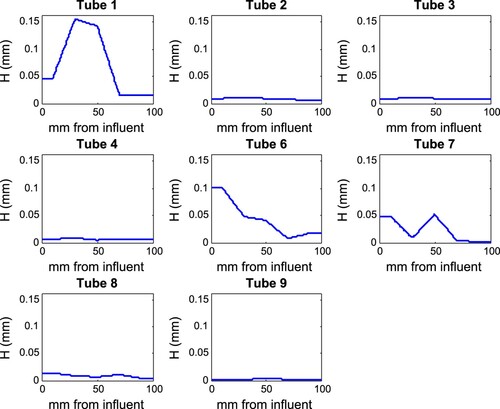
To find biofilm thickness, each 10 cm tube was cut into five 2 cm sections. Each section was cut in half lengthwise, filled with cryoembedding medium, and frozen on dry ice. Once frozen, the silicone tube was peeled off the frozen medium, which was frozen into a larger cutting medium mold for cryosectioning. These frozen samples were cut in 5 μm cross sections and mounted on microscope slides. Each tube segment was used to create 5 cross sections for analysis. An example of these data is shown in Figure 2.

Figure 2. Biofilm height profiles for surviving reactors. Biofilm height profiles H from each of the eight reactors which survived the entire growth, sampling, and cryosectioning process used in the Bayesian statistical analysis.

2.4. Synthetic data

We simulated two sets of synthetic data. We will analyse these synthetic data and use the insights to better understand and interpret the results for real data. The first step in creating the synthetic data $u_L$ was to simulate effluent urea concentrations using the forward problem (FP2) with chosen parameter values for θ. Random normal noise, $ϵ\sim N(0,{\sigma }^2)$, was then added via $u_L=g(\theta ;u^0,H)+ϵ$ to simulate noisy ‘jittered’ data consistent with the error model described in Section 2.1.4. Estimates from preliminary experimental results suggested using a value of $\sigma =1\times {10}^{-4}$ in the simulations. The values used for the parameters $\theta =(r_0,k_m)$ were consistent with measurements of data from preliminary experimental results, $r_0=50\times {10}^{-3}$ mg/(mm³ hr) and $k_m=10\times {10}^{-3}$ mg/mm³. Numerical simulation showed that, for these values of θ and σ, the location and precise thickness of biofilm H in the reactor was relatively unimportant as compared to the total biomass, so uniform flat profiles of the biofilm height 0.1 mm were used. Different influent concentrations $u^0$ were used for the two data sets.

The first synthetic data set, which we will refer to as ‘SD1,’ was used to test the NLS approach to parameter estimation and to demonstrate an important requirement of useful data. These data were created using a single influent concentration of $u^0=0.5\times {10}^{-3}$ mg/mm³ and is available in Table S1 of the Supplementary Materials. The second data set (SD2) was used to test both NLS and Bayesian approaches to solving the inverse problem. To create SD2, five influent concentration values were used, namely, ${\mathbf{u}}^0=(0.5,5,10,15,20)\times {10}^{-3}$ mg/mm³. These data are available in Table S2 of the Supplementary Materials.

2.5. Implementation

Solving the forward model and parameter estimation were performed using Matlab 2019a. Code was auto-parallelised by Matlab and run on 10 Xeon E5-2860 2.8 GHz processors. The unified model solver utilised an upwind scheme in the axial dimension and was discretised using 200 steps. In the case of real data, described in Section 3.2, a chain of length 1000 using eight tube reactors took approximately one second to run for first-order kinetics (IP2) and 400 seconds for Michaelis–Menton Kinetics (IP1 and IP3). Note that the increase in computational time for Michealis-Menton kinetics is due to the need to solve 1600 boundary value problems per evaluation of the forward problem.

Differential equations in the biofilm model were solved explicitly in the case of first-order kinetics (FP1), while Matlab's bvp4c solver was used for Michaelis–Menten kinetics (FP2). Inverse problem solutions and confidence intervals for NLS were computed using lsqnonlin or nlinfit.

The Bayesian solution of the inverse problem (IP3) is based on a Markov chain of samples from the posterior using MCMC. To calculate each element of the chain, the posterior (10(10) $P(\theta ,{\sigma }^2\mid u_L)\propto P(u_L\mid \theta ,{\sigma }^2)P(\theta ,{\sigma }^2)=P(u_L\mid \theta ,{\sigma }^2)P_0\left(\theta \right)P_0\left({\sigma }^2\right).$(10) ) is evaluated. To evaluate the prior for ${\sigma }^2$ in (11(11) $P_0({\sigma }^2\mid \nu ,{\hat{\sigma }}^2)=\left\{\begin{array}{ll}\frac{2^{-\nu /2}}{\mathrm{\Gamma }\left(\nu /2\right)}{\left({\hat{\sigma }}^2\nu /{\sigma }^2\right)}^{\nu /2-1}{e}^{-{\hat{\sigma }}^2\nu /\left(2{\sigma }^2\right)}& \mathrm{i}\mathrm{f}{\sigma }^2>0,\\ 0& \mathrm{o}\mathrm{t}\mathrm{h}\mathrm{e}\mathrm{r}\mathrm{w}\mathrm{i}\mathrm{s}\mathrm{e},\end{array}\right.$(11) ), an estimate of the sample variance ${\hat{\sigma }}^2$ is needed. This is obtained by pooling the variance of the effluent values using the Satterthwaite approximation [40]. For example, for the synthetic data SD2, the pooled estimate for the variance is ${\hat{\sigma }}^2=3.0\times {10}^{-9}$.

We use one of the earliest and simplest MCMC methods, the Metropolis Algorithm, which was first described by Nicholas Metropolis and colleagues in 1953 [41]. We follow the implementation in [42, p.288] using a symmetric uniform proposal distribution. For higher dimensional problems, there are more sophisticated algorithms beyond Metropolis' 1953 scheme. For example, one could apply an adaptive MCMC that uses a normal proposal with mean and covariance that depend on previous samples in the chain [43]. Or one might consider the ‘t-walk’ [44] that speeds convergence by utilizing specialized proposals for sampling the posterior.

To make an initial assessment of the convergence of the Markov chains, the integrated autocorrelation time (IACT) was computed using Matlab code by Wolff [45,46]. To further assess convergence, the potential scale reduction factor ($\hat{R}$) was calculated by comparing multiple parallel chains [35, p. 296–297]

3. Results and discussion

3.1. Parameter estimation from synthetic data

To better understand the strengths and limitations of the NLS and Bayesian approaches to fitting our forward model (FP2) to real experimental data of E. coli biofilms, in this section we analyse two sets of synthetic data. Analysing these synthetic data also helps in interpreting the results from our analysis of real data. Where possible, we will compare conventional confidence intervals from NLS to credible intervals from the Bayesian analysis.

In Case 1, we use NLS to solve (IP1). That is, we use NLS to fit the Michaelis–Menten kinetic model to the SD1 data and show that when our influent concentrations do not span a sufficiently large range, we cannot find a unique estimate value of ${\theta }_{\mathrm{n}\mathrm{l}\mathrm{s}}$. In Case 2, we again consider (IP1), but this time consider the influent concentrations over a sufficiently wide range and use NLS on the SD2 data to find point estimates and confidence intervals for θ. In Case 3, we show that explicitly calculating the posterior distribution (for IP1) on a grid using SD2 data yields point estimates for θ comparable to NLS. However, this case illustrates the lack of symmetry of the resulting credible intervals, showing that NLS confidence intervals are incorrect. In Cases 1–3, it was assumed that σ was known. The final Case 4 illustrates, again using SD2 data, how the Bayesian approach is able to solve the inverse problem (IP3) when ${\sigma }^2$ is not known.

3.1.1. Case 1

The least squares cost function shown in (8(8) $c\left(\theta \right)=\parallel ({\mathbf{u}}_L-{\hat{\mathbf{u}}}_L){\parallel }_2^2.$(8) ) was minimised to find parameter estimates ${\theta }_{\mathrm{n}\mathrm{l}\mathrm{s}}$ for θ that best fit the model to the data SD1 (IP1). In this scenario the solver is sensitive to the initial guess ${\theta }_0$, and different starting values result in different values for ${\theta }_{\mathrm{n}\mathrm{l}\mathrm{s}}$. This is a well known issue with NLS that can occur when there are multiple, distinct local extrema. In our case there is a continuum of points that minimize the cost function along a line in the parameter space (i.e. a valley) with slope given by $k_m/r_0$.

In hindsight the reasons for these nonunique minima are clear and illustrate a difficulty when solving the problem under consideration here. If $u^0\ll k_m$ then, since $s<u^0$, Michaelis–Menten kinetics within the biofilm are well approximated by linear kinetics as (13) $r\left(s\right)=\frac{r_{0}s}{k_m+s}\approx \frac{r_0}{k_m}s=k_{1}s.$(13) On the other extreme, for $u^0\gg k_m$, we have s≫k_m and $r\left(s\right)=\frac{r_{0}s}{k_m+s}\approx \frac{r_{0}s}{s}=r_0$. In this case, $u^0=1\times {10}^{-3}$ is an order of magnitude smaller than the chosen $k_m$. The true effluent value is smaller yet. Thus, urea concentrations in the simulated reactor are always much less than the half-saturation $k_m$. The addition of biofilm further decreases urea in the tube, and thus the model's Michaelis–Menten kinetics are well approximated by first-order kinetics where the first-order rate is $k_1\approx r_0/k_m$. We verified this prediction by calculating the Hessian (matrix of second derivatives) at ${\theta }_{\mathrm{n}\mathrm{l}\mathrm{s}}=[r_0,k_m{]}_{\mathrm{n}\mathrm{l}\mathrm{s}}$ and verified that it is numerically singular (i.e. has eigenvalues close to zero) with a null space that precisely defines the valley of minima along the vector $[r_0,k_m{]}_{\mathrm{n}\mathrm{l}\mathrm{s}}$. As will be shown in the next example, the lack of a unique minimum of the cost function can to some degree be mitigated by generating (synthetic or experimental) data that bracket the possible range of $k_m$ values. That is, we must use data which contain $u_L$ values which are both below and above the actual value of $k_m$.

3.1.2. Case 2

Using NLS to fit Michaelis–Menten kinetics to the data SD2 (IP1), which was created using a wider range of influent concentrations compared to SD1, yields a unique solution ${\theta }_{\mathrm{n}\mathrm{l}\mathrm{s}}$ for each of the next two scenarios. The first scenario is to to validate NLS applied to the complete data set of 15 synthetic data points. In the second scenario, the synthetic replicates for each influent concentration are averaged together to create a single mean effluent concentration for each influent concentration. NLS is then validated when applied to these averaged values. The advantage of the calculation in the second scenario on five data (i.e. five means) is that it is computationally cheaper than using the complete set of 15.

In both scenarios, NLS found a unique minimum at $r_0=64\times {10}^{-3}$ mg/(mm³ hr) and $k_m=18.8\times {10}^{-3}$ mg/mm³ for (8(8) $c\left(\theta \right)=\parallel ({\mathbf{u}}_L-{\hat{\mathbf{u}}}_L){\parallel }_2^2.$(8) ) from a range of starting values. Note that this value is shifted by the presence of noise from the true value of $r_0=50\times {10}^{-3}$ mg/(mm³ hr) and $k_m=10.0\times {10}^{-3}$ mg/mm³. However, the true values fall within the 95% confidence intervals, which are $[46.3,82.6]\times {10}^{-3}$ mg/(mm³ hr) for $r_0$ and $[9.68,28.1]\times {10}^{-3}$ mg/mm³ for $k_m$. It follows that parameterising using this methodology requires data which contain $u_L$ values both below and above the actual value of $k_m$. 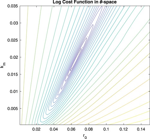The difficulty for experimenters is that often the true value of $k_m$ is unknown. Otherwise, the minima can be difficult to find numerically and convergence may still be sensitive to the initial guess. Figure 3 shows that the minimum exists in a valley that is steep in one direction and shallow in the other, so that the NLS solver may find the valley correctly, but not converge to the minimum in the valley. In fact, different NLS solver implementations have different levels of success locating the minimum, especially with a poor initial guess or badly spread effluent values. Second, (and perhaps more importantly) using simple cost minimisation via NLS we can only assign symmetric and normal confidence intervals around the NLS estimate ${\theta }_{\mathrm{n}\mathrm{l}\mathrm{s}}$. However, we do not necessarily expect that ${\theta }_{\mathrm{n}\mathrm{l}\mathrm{s}}$ will be normally distributed. If the distribution of ${\theta }_{\mathrm{n}\mathrm{l}\mathrm{s}}$ is not normal, but asymmetric as suggested by Figure 3, then a symmetric confidence interval is incorrect and potentially misleading. These shortcomings motivate the Bayesian approach to the inverse problem.

Figure 3. NLS cost function. A plot of the cost function (8(8) $c\left(\theta \right)=\parallel ({\mathbf{u}}_L-{\hat{\mathbf{u}}}_L){\parallel }_2^2.$(8) ) in $(r_0\times k_m)$ space close to minimum ${\theta }_{\mathrm{n}\mathrm{l}\mathrm{s}}$ found by NLS for the synthetic data in Case 2. Cost contours around the minimum at $(49.2,4.50)\times {10}^{-3}$ demonstrate a lack of symmetry. This results in incorrect and misleading NLS confidence intervals.

3.1.3. Case 3

Explicitly computing the posterior (12(12) $P(\theta \mid u_L,{\sigma }^2)=\left\{\begin{array}{ll}\frac{P(u_L\mid \theta ,{\sigma }^2)P_0\left(\theta \right)}{P\left(u_L\right)},& \mathrm{i}\mathrm{f}\theta \in I_{r_0}\times I_{k_m},\\ 0& \mathrm{o}\mathrm{t}\mathrm{h}\mathrm{e}\mathrm{r}\mathrm{w}\mathrm{i}\mathrm{s}\mathrm{e}.\end{array}\right.$(12) ) using synthetic data SD2 (IP1) allows us to plot the posterior space as shown in Figure 4 (A), with a summary in Table 2. Comparison of these plots with the earlier log cost plot shown in Figure 3 shows that the long low-cost valley now manifests in the posterior as a long ridge of elevated probability densities. This feature causes the marginal distributions, shown in Figures 4(B) and 4(C), to be right-skewed. This in turn results in the marginal posterior MAP and median estimates for $r_0$ and $k_m$ being greater than the true values (Table 2). Not surprisingly, it is possible to sharpen the posterior peak and reduce the right-skewedness of the marginal posteriors by reducing the amount of noise in the data (i.e. by averaging). In an experiment, this could be done by adding additional tubes at each concentration and then analysing the mean for each influent concentration.

Figure 4. Bayesian posterior when σ is known. These plots summarise the output of the Case 3 synthetic data example. The posterior $P\left(u|\theta \right)$ was computed explicitly on a grid in the parameter space, $\theta =[r_0,k_m]$. Pane (A) shows a 3D representation of the posterior distribution. Panes (B) and (C) show the $r_0$ and $k_m$ marginal posterior distributions, respectively. The shaded pink areas in (B) and (C) are the 95% credible intervals for $r_0$ and $k_m$, respectively. The vertical dashed line shows the median value for each marginal distribution. These results are summarised in Table 2.

Table 2. Bayesian estimates for kinetic parameters when σ is known.

	$r_0\times {10}^{-3}$ mg/(mm^3 hr)	$k_m\times {10}^{-3}$ mg/mm^3
True value	50	10
Marginal MAP	66	20
95% credible interval	$[51,93]$	$[12,33]$
Marginal posterior median	69	21

Note: Various estimates for $r_0$ and $k_m$, derived from the Bayesian posterior $P(\theta \mid u)$ applied to synthetic data with averaged effluent concentrations (Case 3).

3.1.4. Case 4

In the previous cases we assumed that the variance was known. In this case, which simulates analyses of real data, we acknowledge that σ is unknown and estimate it as well as θ from the Bayesian posterior using MCMC. That is, we will analyse the data with first-order (IP2) and Michaelis–Menten (IP3) kinetics.

We begin by solving (IP3) by sampling from the posterior (10(10) $P(\theta ,{\sigma }^2\mid u_L)\propto P(u_L\mid \theta ,{\sigma }^2)P(\theta ,{\sigma }^2)=P(u_L\mid \theta ,{\sigma }^2)P_0\left(\theta \right)P_0\left({\sigma }^2\right).$(10) ) using a simple Metroplis MCMC method (Section 2.5) given the same synthetic data SD2 from Case 3. Even though we generated these synthetic data by Michaelis–Menten kinetics (via (FP2)) using fixed values of θ (see Section 2.4), this case confirms what we observed when studying Case 1–3, that in the presence of noise, there is a high correlation between highly probable solutions to the Michealis-Menten model parameters (i.e. there is a long ridge in the posterior). In this case we also consider results from a simpler first-order model (FP1) fit to the data. This is the same situation that an experimenter might encounter when analysing real data. Not knowing which kinetics model to use, the experimenter may like to fit more than one kinetics model to the same data (see our analysis of real data in Section 3.2).

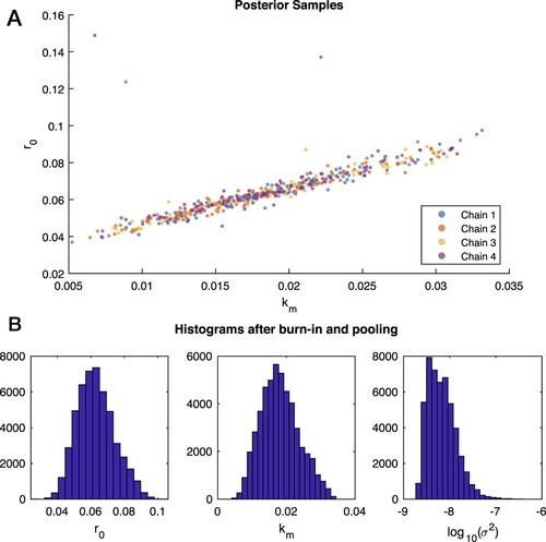
Four Markov chains of the parameters were run for T = 25, 000 iterations, each from a random start. These are very long chains for only a 3D inverse problem (IP3), but they were used to assure convergence. The acceptance rate was 11%. Viewing the chains in the 2D support for $r_0$ and $k_m$ in Figure 5(A) clearly indicates convergence of all 4 chains to the posterior, that the posterior has a long ridge (as expected from Cases 2–3), and that the chains mix well (i.e. samples from different chains overlay; see, e.g. [47]). Other graphical assessments of the chains in Figure S1 and a discussion of convergence assessment are provided in the Supplementary Material.

Figure 5. Samples from Bayesian posterior when σ is not known. A: A 2D plot of $k_m$ versus $r_0$ for the four chains computed by MCMC for Case 4 synthetic data. The chains exhibit good mixing and convergence to the thin ridge of the posterior. In this plot every 200th sample from the chains is shown. B: Frequency histograms for each parameter from the Markov chains in Case 4 after the exclusion of the first half of each chain as burn-in values and the pooling of parallel chains.

To quantitatively assess convergence, a potential scale reduction, $\hat{R}$ was calculated, which measures the factor by which the scale of the present distribution for each parameter might be reduced by additional draws [35]. If $\hat{R}$ is near 1, additional simulations will not move the present distribution and in practice, one may conclude the Markov chains have converged. For practical purposes, values of $\hat{R}$ below 1.1 are deemed sufficiently close to 1 [35, p. 297]. Here, $\hat{R}=1.01$ for each of the three parameters, which confirms that the chains have converged.

The auto correlation times for the three parameters are long (309, 338, and 594 for $r_0$, $k_m$, and ${\sigma }^2$, respectively) indicating that it takes 309–594 consecutive samples in the chain to generate a new independent sample.

The chains are summarised in Figure 5. In the upper pane (A), every 200th element of the chain is plotted. In the lower pane (B), the first half of each chain was discarded as burn-in, and the remaining halves were pooled to 50,000 samples that we treat as samples from the posterior. The lower half of Figure 5 shows histograms of these samples with properties summarized in Table 3.

Table 3. Bayesian estimates of kinetic parameters when σ is not known.

	$r_0\times {10}^{-3}$ mg/(mm^3 hr)	$k_m\times {10}^{-3}$ mg/mm^3	${\sigma }^2\times {10}^{-9}$ (mg/mm^3)^2
True value	50	10	10
Marginal MAP	63	17	3.6
Marginal posterior median	62	18	6.2
95% credible intervals	$[46,83]$	$[10,28]$	$[2.7,24]$

Note: A summary of MCMC results using synthetic data in Case 4 with averaged effluent values and unknown variance. The credible intervals contain the true parameter values used to generate the data.

One of the strengths of our model is the ability to incorporate different kinetic models (FP1) and (FP2). Although we generated the synthetic data in this case with Michaelis–Menten kinetics, we wanted to see how the first-order model would fit. If the urea concentration in the biofilm is small compared to the kinetics parameters, then $k_1$ should be close to the ratio of $r_0$ to $k_m$ as shown in (13(13) $r\left(s\right)=\frac{r_{0}s}{k_m+s}\approx \frac{r_0}{k_m}s=k_{1}s.$(13) ). Alternatively, if the biofilm metabolises urea very slowly, or if the urea levels are large compared with the kinetic values of $r_0$ and $k_m$, then $k_1$ should be unrelated.

Applying the Bayesian approach to solve (IP2) using MCMC for 1st-order kinetic parameter $k_1$, a clear burn-in period is followed by convergence of the chain to a median and MAP value of $k_1=1.9$ hr⁻¹ with a 95% credible interval of $[1.6,2.2]$ hr${}^{-1}$ (chain not shown). In comparison, the MAP ratio in Table 3 shows that ${\hat{r}}_0/{\hat{k}}_m=63/17=3.7$ (we also considered the posterior for the ratio $r_0/k_m$, which gave a similar estimate). The 95% credible interval for σ is $[0.13,0.34]\times {10}^{-3}$ mg/mm³. Thus, despite the convergence of the method, the first-order parameter is quite different than the ratio of Michaelis–Menten parameters. This shows that the ratio of $r_0$ to $k_m$ is not a good approximation of $k_1$ in this scenario. Of course, with real experimental data we would not have inside knowledge about the generating kinetics. Because both kinetics models result in solvable inverse problems, this simulation demonstrates that experimenters would do well to consider multiple possibilities when fitting kinetic data.

3.2. Parameter estimation from real experimental data

Based on our experience from the application of our approach to synthetic data, we now fit Michaelis–Menten kinetics (IP3) to real urea data from experiments on E. coli biofilms. These data consisted initially of twelve tube reactors, three at each target influent concentration of 0.5, 5, 10, and 15 g/L of urea. Eight of these tubes were deemed to have reached steady state and are used here in the subsequent modelling. The influent and effluent concentration data from these reactors are tabulated in [6] as well as in Table S3 in the Supplementary Material. The height profiles used for each reactor are shown in Figure 2 and tabulated in the Supplemental Information.

Four Markov chains of the parameters were run for 100,000 iterations using the Metropolis method. The acceptance rate was $23.4\mathrm{\%}$ which should ensure a reasonable exploration of the parameter space [29, p. 174]. The assumed parameter domain was $I_{r_0}\times I_{k_m}\times I_{{\sigma }^2}$, where $\begin{array}{rl}{I}_{r_0}& =[0.001,1.8]\mathrm{m}\mathrm{g}/\left(\mathrm{m}{\mathrm{m}}^3\mathrm{h}\mathrm{r}\right)\\ I_{k_m}& =[0.006,0.06]\mathrm{m}\mathrm{g}/\mathrm{m}{\mathrm{m}}^3\\ I_{{\sigma }^2}& =(0,\mathrm{\infty })(\mathrm{m}\mathrm{g}/\mathrm{m}{\mathrm{m}}^3{)}^2\end{array}$defined the prior $P_0\left(\theta \right)$. The starting vector for each chain was chosen randomly from this domain.

Viewing the 4 chains in the 2D support for $r_0$ and $k_m$ in Figure 6(A) clearly indicates convergence of all 4 chains to the posterior and that the chains mix well (i.e. points overlay). While there is a long ridge as for the idealized synthetic data Case 4 (Figure 5(A)), the posterior based on real experimental data has a larger spread of samples about the upper right-hand section of the ridge. Other graphical assessments of the chains in Figure S3 and a discussion of convergence assessment are provided in the Supplementary Material.

Figure 6. Samples from Bayesian posterior for real experimental data from E. coli biofilms. A: A 2D plot of $k_m$ versus $r_0$ for the four chains computed from real data show good mixing and convergence to the posterior. In this plot every 200th sample in the chains is shown. B: The histograms for $r_0$ and $k_m$ echo the wide range of values shown in pane (A). However, all parameters are grouped around an asymmetric MAP value.

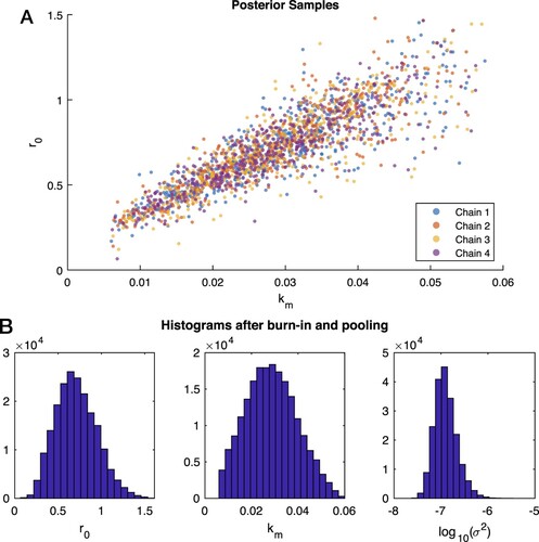
To quantifiably assess convergence, the potential scale reduction was $\hat{R}=1.01$. Because this value is close to 1, it confirms, as in Case 4 with synthetic data, that these chains have converged in distribution. Pooling the retained final 50,000 simulations from each of the four chains allows the calculation of the results shown in Table 4 and the corresponding histograms in pane (B) of Figure 6. Computing the autocorrelation for each variable gives values of approximately 200 for $r_0$ and $k_m$, and 10 for ${\sigma }^2$. The much longer autocorrelation times for $r_0$ and $k_m$ is due to the existence of the long ridge in the posterior.

Table 4. Bayesian estimates of Michaelis–Menten kinetic parameters for real experimental data.

	$r_0\times {10}^{-3}$ mg/(mm^3 hr)	$k_m\times {10}^{-3}$ mg/mm^3	${\sigma }^2\times {10}^{-9}$ (mg/mm^3)^2
MAP	646	0.029	0.34
Posterior median	695	0.028	0.35
95% credible interval	(346, 1123)	(0.011, 0.047)	(0.24, 0.58)
Connolly estimate	955	0.033	na

Notes: Parameter estimates using MCMC with Michaelis–Menten kinetics on experimental data shown. Results from [6] are given for a comparison as these are the only similar estimates available.

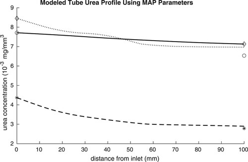
To graphically assess the model fit to data, experimentally measured influent and effluent urea concentrations were compared to the predicted urea profile in several tubes (based on the MAP parameter values from Table 4). These are shown in Figure 7. The difference in the predicted urea profiles across the tubes is driven by the differing biofilm height profiles in Figure 2.

Figure 7. Bayesian predictions of urea profiles inside tube reactors based on real experimental data. Experimental data plotted with modelled urea concentrations for a sample of three tube reactors (solid-circle, dashed-star, and dotted-diamond represent reactors 2, 6 and 7, respectively.). The influent and effluent values indicated by asterisks are measured in the lab. The MAP estimates for $k_m$ and $r_0$ from MCMC were used to generate the curves.

Based on our analysis of synthetic data that also exhibited a long ridge as in Figure 6(A), we also consider the fit of first-order kinetics to these real data. Hence we apply MCMC to estimate the first-order parameter $k_1$ (IP2). When inspecting the chains for the parameters for this inverse problem in Figure S5 in the Supplementary Materials, a burn-in period to T = 2500 is clear. The naive NLS approach and the more sophisticated Bayesian method give similar results, see Table 5. Comparing this result to the Michaelis–Menten results, it is telling that the ratio of $r_0$ and $k_m$ values is reasonably close to the 1st-order estimates for $k_1$. Using the MAP values from Table 4 we find $r_0/k_m=0.646/0.029=22.3$ hr⁻¹. (The posterior for the ratio $r_0/k_m$ gave a similar estimate.) This value is in the 95% credible intervals from Table 5. It appears that for these data the first-order parameter $k_1$ is approximately the ratio of these two parameters. One reason for this similarity is that the biofilms in this experiment may be thin enough that a first-order approximation for ureolytic kinetics is more appropriate than Michaelis–Menten kinetics. Alternatively, the MAP value of $r_0$ shown in Table 4 are quite large in comparison to $k_m$ and the influent concentration of urea. This means that urea entering the biofilm is quickly metabolised, meaning urea concentration is very low in the biofilm away from the boundary. Thus, as shown in in (13(13) $r\left(s\right)=\frac{r_{0}s}{k_m+s}\approx \frac{r_0}{k_m}s=k_{1}s.$(13) ), first-order kinetics are a good approximation for Michaelis–Menten kinetics.

Table 5. Bayesian estimates of first-order kinetic parameters for real experimental data.

	$k_1$ (hr^-1)	σ (${10}^{-3}$ mg/mm^3)
NLS estimate	19.1	0.27
NLS 95% confidence interval	(14.3, 24.0)	na
MCMC Marginal MAP estimate	19.7	0.29
MCMC Marginal posterior median	19.2	0.28
MCMC 95% credible interval	(15.4, 23.1)	(0.19, 0.46)
$\tau Int$	5.0	3.8
Connolly estimate	23.2	na
Connolly 95% confidence interval	(17, 29.4)	na

Notes: Here NLS results are compared to MCMC results. As before, comparison with Connolly et al. is made as these are the only similar estimates available.

Instead of fitting the first-order model to these data, another option would be to use a more informative prior for the Michaelis–Menten parameters. That is, instead of the prior specifying that possible values of the parameters are uniformly distributed between upper and lower bounds as we do here, we could, for example, assume a prior normal distribution of the parameters around a mean value calculated from previous experiments (see [48]). This is a topic for further research.

4. Conclusions

Biofilms are ubiquitous in natural and artificial systems. Many natural and artificial systems involve water flowing over a microbial mat. Despite advances in imaging and experimental sophistication, mathematical models continue to play an important role in studying how material is transported in systems where biofilm are present.

In this paper we have exhibited a tube reactor model comprising two coupled 1-dimensional models to describe the consumption of the substrate urea by a biofilm growing in a tube or in a long, narrow pore-space. This unified model is flexible with respect to the kinetics used (i.e. first order or Michaelis–Menten) in the biofilm, and is able to make use of biofilm height profile data from experiments. This allows modellers to account for model and experimental uncertainty explicitly in the form of a statistical likelihood function. When nonlinear least squares was not able to solve the inverse problem, we developed a Bayesian method which could.

The goal of our research was to develop a realistic model of urea utilization, to fit the model to real experimental data generated by E. coli biofilms grown in the lab, and to assess the fit of the model to the data. Our use of synthetic data assisted in performing this final step and in interpreting the results from real data. In general, modellers ought to be cautious when interpreting results from fitting a model to synthetic data because the model will tend to fit well. Nonetheless, such simulation studies are a first step towards identifying poor models or a poor approach to solving an inverse problem. In our case, the simulation study allowed us to determine that, even when Michaelis–Menten was the ‘true’ model for generating noisy synthetic urea data, first-order kinetics can also fit the data well.

Experimenters should take away four important lessons from this work. First, though commonly used, NLS is not always an appropriate method to solve inverse problems. Not only might the solution heavily depend on the initial parameter estimates used, but equally important, the posterior probability distribution is not necessarily symmetric, an implicit assumption of NLS. If this is the case, the confidence interval returned by NLS may be incorrect and misleading. A second lesson is that for resolving Michaelis–Menten kinetic parameters, mitigating measurement error by sufficient replication is critical. Because the sampling variance is inversely proportional to the number of tubes that are used, we recommend that experimenters employing these techniques use as many tube reactors as is physically practical. Stated more generally, replication is crucial for parameter estimation. A third point is that, models can only resolve Michaelis–Menten kinetic parameters when the data include a range of effluent concentrations that include the half-saturation, $k_m$. Given that the value for $k_m$ may not be known, it behooves the experimenter to include as wide a range of influent concentrations as possible or first attempt to measure $k_m$ directly.

The fourth and final point is that when trying to fit Michaelis–Menten kinetics, the data may more readily determine first-order kinetics. A strength of our modelling approach is that it allows both types of kinetics models to be fit and compared. When the first-order parameter is approximately the ratio of Michaelis–Menten parameters, this suggests that the range of urea concentrations observed is not wide enough, or that the urea concentrations are too low compared to the kinetic rates. If the first-order rate is not similar to the ratio, then this could indicate that either the biofilm metabolises urea very slowly or that the urea levels are large compared with the kinetic values of the Michaelis–Menten parameters. To determine which of these scenarios is the case, the experimenter can fit both types of kinetic models using our flexible modelling approach. In either case, our analyses found a long steep ridge in the posterior indicating highly probable Michaelis–Menten parameter values. This high steep ridge could be a substantial contributing factor to why others [49,50] have found that the Michaelis–Menten kinetic model can be unidentifiable when fitting to noisy data. In general, parameters may be unidentifiable when there is not enough data, when the data are too noisy, or if the proposed model does not match reality.

Disclosure statement

No potential conflict of interest was reported by the author(s).

Additional information

Funding

This research was funded by National Science Foundation (NSF) grant numbers 0934696,1517100. We also acknowledge the German Research Foundation Deutsche Forschungsgemeinschaft (DFG) through grant number 380443677 and the Collaborative Research Centre 1313, as well as the U.S. Department of Energy grant number DE-SC0010099.

References

- Stickler DJ. Bacterial biofilms in patients with indwelling urinary catheters. Nat Clin Pract Urol. 2008;5(11):598–608.
- Espinosa-Ortiz EJ, Eisner BH, Lange D, et al. Current insights into the mechanisms and management of infection stones. Nat Rev Urol. 2019;16(1):35–53.
- De Muynck W, De Belie N, Verstraete W. Microbial carbonate precipitation in construction materials: a review. Ecol Eng. 2010;36(2):118–136.
- Phillips AJ, Gerlach R, Lauchnor E, et al. Engineered applications of ureolytic biomineralization: a review. Biofouling. 2013;29(6):715–733.
- Yingjie Q, Cabral JM. Review properties and applications of urease. Biocatal Biotransfor. 2002;20(1):1–14.
- Connolly J, Gerlach R, Jackson B, et al. Estimation of a biofilm-specific reaction rate: kinetics of bacterial urea hydrolysis in a biofilm. NPJ Biofilms Microbiomes. 2015;1:15014.
- Lauchnor EG, Topp D, Parker A, et al. Whole cell kinetics of ureolysis by s porosarcina pasteurii. J Appl Microbiol. 2015;118(6):1321–1332.
- Tobler DJ, Cuthbert MO, Greswell RB, et al. Comparison of rates of ureolysis between Sporosarcina pasteurii and an indigenous groundwater community under conditions required to precipitate large volumes of calcite. Geochim Cosmochim Acta. 2011 Jun;75(11):3290–3301.
- Ebigbo A, Phillips A, Gerlach R, et al. Darcy-scale modeling of microbially induced carbonate mineral precipitation in sand columns. Water Resour Res. 2012;48(7):433.
- Redden G, Fox D, Zhang C, et al. Caco3 precipitation, transport and sensing in porous media with in situ generation of reactants. Environ Sci Technol. 2013;48(1):542–549.
- Moynihan H, Lee C, Clark W, et al. Urea hydrolysis by immobilized urease in a fixed-bed reactor: analysis and kinetic parameter estimation. Biotechnol Bioeng. 1989;34(7):951–963.
- Caers J, Hoffman T. The probability perturbation method: a new look at Bayesian inverse modeling. Math Geol. 2006;38(1):81–100.
- McLaughlin D, Townley LR. A reassessment of the groundwater inverse problem. Water Resour Res. 1996;32(5):1131–1161.
- Beck JL, Katafygiotis LS. Updating models and their uncertainties. I: Bayesian statistical framework. J Eng Mech. 1998;124(4):455–461.
- Wang J, Zabaras N. Hierarchical Bayesian models for inverse problems in heat conduction. Inverse Probl. 2004;21(1):183–206.
- Ma R, Liu J, Jiang Yt, et al. Modeling of diffusion transport through oral biofilms with the inverse problem method. Int J Oral Sci. 2010;2(4):190–197.
- Rao KR, Srinivasan T, Venkateswarlu C. Mathematical and kinetic modeling of biofilm reactor based on ant colony optimization. Process Biochemistry. 2010;45(6):961–972.
- Chen-Charpentier B, Stanescu D. Parameter estimation using polynomial chaos and maximum likelihood. Int J Comput Math. 2014;91(2):336–346.
- Younes A, Delay F, Fajraoui N, et al. Global sensitivity analysis and bayesian parameter inference for solute transport in porous media colonized by biofilms. J Contam Hydrol. 2016;191:1–18.
- Oyebamiji OK, Wilkinson DJ, Jayathilake PG, et al. A Bayesian approach to modelling the impact of hydrodynamic shear stress on biofilm deformation. PLoS ONE. 2018;13(4):1–21.
- Wahlen L, Parker A, Walker D, et al. Predictive modeling for hot water inactivation of planktonic and biofilm-associated sphingomonas parapaucimobilis to support hot water sanitization programs. Biofouling. 2016;32(7):751–761.
- Parker RL. Understanding inverse theory. Annu Rev Earth Planet Sci. 1977;5(1):35–64.
- Stewart PS. Diffusion in Biofilms. J Bacteriol. 2003;185(5):1485–1491.
- Gosting L, Akeley D. A study of the diffusion of urea in water at 25 C with the Gouy interference method. J Amer Chem Soc. 1952;74(8):2058–2060.
- Smith RC. Uncertainty quantification: theory, implementation, and applications. Philadelphia: SIAM; 2014.
- Bardsley JM. Computational uncertainty quantification for inverse problems. Philadelphia: SIAM; 2018.
- Fox C, Norton R. Fast sampling in a linear-Gaussian inverse problem. J Uncertainty Quantif. 2016;4:1191–1218.
- Bernardo J, Smith A. Bayesian theory. New York: John Wiley and Sons; 1994.
- Calvetti D, Somersalo E. Introduction to Bayesian scientific computing: ten lectures on subjective computing. Springer; 2007. (Surveys and Tutorials in the Applied Mathematical Sciences; 2).
- Casella G, Berger R. Statistical inference. Belmont (CA): Duxbury Press; 1990.
- Kim SH. Statistics and decisions: an introduction to foundations. New York: Van Nostrand Reinhold; 1992.
- Link W, Barker R. Bayesian inference with ecological applications. Boston: Academic Press; 2010.
- Tenorio L. An introduction to data analysis and uncertainty quantification for inverse problems. Philadelphia: SIAM; 2017.
- Wackerly DD, Mendenhall W, Scheaffer RL. Mathematical statistics with applications. 7th ed. Belmont (CA): Brooks Cole; 2008.
- Gelman A, Carlin JB, Rubin DB. Bayesian data analysis. 2nd ed. Chapman & Hall CRC; 2004. (Texts in Statistical Sciences).
- Higdon D. A primer on space-time modelling from a Bayesian perspective. In: Finkenstadt B, Held L, Isham V, editors. Statistics of spatio-temporal systems. New York: Chapman & Hall/CRC; 2006. p. 217–279.
- Bates DM. lme4: Mixed-effects modeling with r; 2010.
- Efron B, Tibshirani RJ. An introduction to the bootstrap. Philadelphia: CRC press; 1994.
- Connolly J, Kaufman M, Rothman A, et al. Construction of two ureolytic model organisms for the study of microbially induced calcium carbonate precipitation. J Microbiol Methods. 2013 Sep;94(3):290–299.
- Satterthwaite F. An approximate distribution of estimates of variance components. Int Biom Soc. 1946;2(6):110–114.
- Metropolis N, Rosenbluth AW, Rosenbluth MN, et al. Equation of state calculations by fast computing machines. J Chem Phys. 1953;21(6):1087–1092.
- Roberts C, Casella G. Monte Carlo statistical methods. 2nd ed. New York: Springer; 2004.
- Haario H, Saksman E, Tamminen J. Adaptive proposal distribution for random walk metropolis algorithm. Comput Stat. 1999;14(3):375.
- Christen J, Fox C. A general purpose sampling algorithm for continuous distributions (the t-walk). Bayesian Anal. 2010;5(2):263–281.
- Wolff U. Monte Carlo errors with less errors. Comput Phys Commun. 2004 Jan;156(2):143–153.
- Wolff U. Erratum to ‘Monte Carlo errors with less errors’ [Comput Phys Comm. 156 (2004) 143–153]. Comput Phys Commun. 2007 Mar;176(5):383.
- Peltonen J, Venna J, Kaski S. Visualizations for assessing convergence and mixing of Markov chain Monte Carlo simulations. Comput Stat Data Anal. 2009;53(12):4453–4470.
- Heino J, Calvetti D, Somersalo E. Metabolica: a statistical research tool for analyzing metabolic networks. Comput Methods Programs Biomed. 2010;97:151–167.
- Choi B, Rempala GA, Kim JK. 2017. Beyond the Michaelis–Menten equation: accurate and efficient estimation of enzyme kinetic parameters. (Scientific Reports. 7).
- Holmberg A. On the practical identifiability of microbial growth models incorporating Michaelis–Menten type nonlinearities. Math Biosci. 1982;62(1):32–43.