Analysis for two-dimensional inverse quasilinear parabolic problem by Fourier method

Abstract

In this work, two-dimensional inverse quasi-linear parabolic problem with periodic boundary and integral overdetermination conditions is investigated. The formal solution is obtained by the Fourier approximation. Under some natural regularity and consistency conditions on the input data,the existence, uniqueness and continuously dependence upon the data of the solution are proved by iteration method. The inverse problem is first examined by linearization and then used implicit finite difference scheme for the numerical solution. Also predictor corrector method is considered in the numerical approach. Some results on the numerical solution with two examples are presented with figures and tables. The sensitivity of the scheme with respect to noisy overdetermination data is illustrated.

Keywords:

• Inverse problem
• two-dimensional heat problem
• periodic boundary conditions

AMS Subject Classifications:

• 35K55
• 35K70

Nomenclature

	=	Initial function
	=	Unknown coefficient
	=	Energy function
	=	Temperature distribution
	=	Heat flux
	=	Source function
	=	Lipschitzs coefficients
	=	Fourier coefficients
	=
M	=	Arbitrary constant
	=	Dimensionless constants
Γ	=	Domain of x, y, t
D	=	Domain of x, y
	=	integral variables
	=	spatial variables
t	=	time variable
T	=	upper bound of t

1. Introduction

Inverse problems in a parabolic equation arise in the study of mathematical models for many important applications such as chemical diffusion, applications in heat conduction processes, population dynamics, medical area, electrochemistry, thermoelasticity, engineering, wide scope, plasma physics, a response of this object or medium, to a probing signal [1,2].

Recently, the development of the two-dimensional parabolic problems has been an important research topic in many branches of science and engineering. In [3], an inverse problem for a two-dimensional degenerate heat equation in a rectangular domain is considered. The existence and uniqueness of solutions in the problem of identifying the leading coefficient is presented by applying Schauder fixed-point theorem. In [4,5], the two-dimensional linear parabolic partial differential equations with nonclassical boundary conditions are considered. A numerical approach is presented with finite difference techniques. Sharma investigates solution of two-dimensional linear parabolic partial differential equation with non-local boundary conditions using Homotopy Perturbation Method (HPM) in [2]. In [6], the model of partial differential equation (PDE) is transformed into a system of first order, linear, ordinary differential equations (ODEs) to obtain solution of the two-dimensional parabolic partial differential equations with nonlocal boundary conditions. In [7], the method of lines semi-discretization approach is used to transform the model PDE into a system of first order, linear, ordinary differential equations (ODE'S), the solution of which satisfies a certain recurrence relation involving matrix exponential terms and subdiagonal Pade approximant is used for numerical solution. In [8], the two-dimensional inhomogeneous diffusion equations subject to a nonlocal boundary condition is solved by transforming the model of partial differential equation (PDE) into a system of first order, linear, ordinary differential equations (ODEs).

Finding of the unknown function in a two-dimensional parabolic equation is also used frequently by many engineers and scientists. In [9], three implicit finite difference schemes are presented for the numerical solution of the inverse two-dimensional parabolic problem in local boundary conditions. In [10], a numerical method based on Haar wavelets is used for solving multidimensional parabolic inverse problem for a control parameter with local boundary condition. In  [11–13], finite difference method is applied for two-dimensional parabolic inverse problems with local boundary condition. Numerical schemes for solving two-dimensional parabolic inverse problem with integral boundary conditions is considered in [14]. Z Meng and Z Zhao [15] a Hermite spectral method for solving a multiple dimensional inverse heat source problem in an unbounded domain and numerical experiments for the one-dimension and two-dimension cases are given.

In this paper, we present two-dimensional nonlinear parabolic inverse problem with periodic boundary and integral overdetermination conditions. Inverse problem for this coefficient which we consider, has not been studied yet with these conditions. Studying with nonlocal conditions in both theoretical and numerical includes difficulties. Because there are much more operations than local conditions.

The differences between current papers are nonlinearity, the type of the unknown coefficient, periodic boundary and integral overdetermination conditions. The periodic boundary conditions arise from many important applications in heat transfer, life sciences and used on lunar theory [16–19].

We prove the existence, the uniqueness and the continuous dependence on the data of the solution and we develop the numerical solution of two-dimensional diffusion problem with periodic boundary conditions. We use Fourier method and the finite difference method for two-dimensional inverse parabolic equation.

The Fourier series analysis of the problems with classical boundary conditions are applicable uneventfully since the expansion in terms of eigenfunctions of auxiliary spectral problem is perfectly studied in varies literature. To study nonlinear parabolic equation with nonlocal boundary condition is difficult in technical point of view. In order to obtain analytical solution of the heat equation, we used the expansion in terms of eigenfunctions for the auxiliary spectral problem corresponding to the considered problem [17,18,20].

The finite difference schemes is considered in this paper. The main idea behind the finite difference methods for obtaining the solution of a given partial differential equation is to approximate the derivatives appearing in the equation by a set of values of the function at a selected number of points. The most usual way to generate these approximations is through the use of Taylor series. The numerical method suggested here is the implicit finite difference method which is second order accurate in the spatial grid sizes and first order in the time grid size. Also the Crank–Nicolson scheme, which is absolutely stable and has a second-order accuracy in the spatial and time grid sizes can be used The Crank–Nicolson scheme require far more computational efforts than the implicit scheme especially in the higher dimensional problems. So the CPU time in the Crank–Nicolson scheme is longer than the implicit finite difference method. The explicit finite difference schemes for the numerical solution of the two-dimensional diffusion equation is the restriction of the size of the time step due to stability requirements.

The article consists of four parts, In Part 2, the existence and uniqueness for the solution is proved by Fourier method and iteration. In Part 3, continuous dependence for the solution is examined. In Part 4, the numerical approximation is given.

Figure 1. Domain .

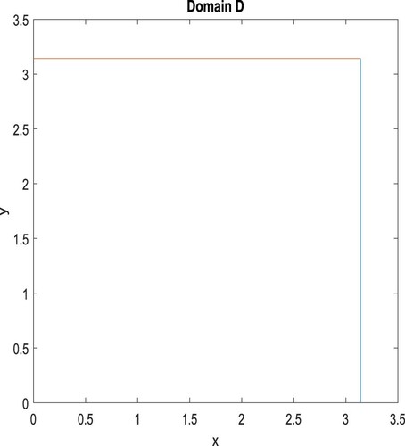
Consider (Figure 1) (1) (2) (3) (4) (5) where are given functions. Clearly, in physical meaning, Equation (1(1) ) is used to describe a heat transfer process. (2(2) ) is initial conditions, (3(3) ) and (4(4) ) are periodic boundary conditions. In heat diffusion in a thin bar in which the law of variation of the total quantity of heat in the bar is given [21].  Condition (5(5) ) is also called heat moments in parabolic problems.

2. Solution of two-dimensional model

As known, in Fourier Method, the solution of problem (1(1) )–(4(4) ) is considered in the following form: (6) First taking the derivative of the last equation with respect to t once and with respect to x, y twice, and substituting this in Equation (1(1) ), we obtain: (7) Now integrating the last equation over the closed interval  twice, we obtain the following form: (8) (9) After obtaining the solution of the last system of equations, we substitute this solution and initial condition (2(2) ) in the above form of , we obtain the solution of the problem (1(1) )–(4(4) ) in the following form: (10) where where

We have Fourier coefficients as follows: (11) where and

We have the following assumptions for the given functions:

(K1)
(K2)	and
(K3)	is provided following conditions: where where is Lipschitzs coefficients, Differentiating (5(5) ) under the assumptions (K1)–(K3), (12) then the unknown coefficient is obtained in this form (13) where

Definition 2.1

Show the set of continuous functions on [0, T] which satisfy the condition is the norm in B. (B is the Banach spaces).

Theorem 2.1

If the conditions (K1)–(K3) be implemented. Then it has a unique solution.

Proof.

If we apply an iteration to Equation (6(6) ), the following functions are obtained: Let us begin the iteration for

If we use Cauchy inequality, we obtain

then using Holder inequality, we have then Bessel inequality, we get

According to the assumptions and using Lipschitzs condition, we get , finally we obtain: According to the assumptions of the theorem, we have . The same operations for the step N, is obtained. We get since If we apply an iteration to Equation (9(9) ), the following functions are obtained: (14) By using the same operations, we have: (15) (16) We get since , .

Let us show that, are converged for If we use Cauchy inequality, we obtain

then using Holder inequality, we have then Bessel inequality, we get

Lipschitzs condition is implemented to the previously inequality, the following estimation are obtained: where Contiuning to the N. step, the following inequality is obtained: By using the same operations, we obtain: where For the step N: The series is uniformly convergent. Therefore, and are converged.

Now let's show that:

Let some inequalities (Cauchy, Hölder) be implemented, we obtain By using Bessel,  we have

by using Lipschitzs condition, we have By using the same operations we obtain: applying Gronwall's inequality to last inequality, we have (17) The series which is consisting of the right hand side of (18(18) ) are convergent by ratio test. So, the series which is consisting of the left hand side of (18(18) ) are convergent by comparison test. Moreover, by the Weierstrass M test, the series is uniformly convergent.

We obtain

To show the uniqueness, we get two solution pairs of the problem (1(1) )–(5(5) ) as and Applying Cauchy inequality, Hölder Inequality, Lipschitzs condition and Bessel inequality to the difference we obtain (18) we get and

The proof is over.

3. Stability of the solution

Theorem 3.1

Under (K1)–(K3), the solution of problem (1(1) )–(5(5) )  depends continuously on the given data.

Proof.

Supposed and , M, i = 1, 2 are positive constants such that Let we take Let and be solutions: By using the same estimations, we obtain where

For then Hence

4. The numerical examination

In this section, firstly we use linearization to obtain a linear problem. Then we use finite difference method and predictor-corrector method to find the numerical solution.

We need to obtain linearization of the nonlinear terms: (19) (20) (21) (22) If we take and then we have a linear problem: (23) (24) (25) (26) is divided to an mesh with the step sizes .

Grid points , are defined by

Let's take and that instead of , and , respectively.

Then we use implicit finite-difference method for problem (26(26) ) and (27(27) ): (27) (28) (29) (33) If we integrate Equation (1(1) ) with respect to x and y from 0 to π and use (3(3) )–(5(5) ), we obtain (30) The approximation function of (32(32) ) is where

We use for the integrals are found numerically according to Simpson's integration rule applying the central difference scheme.

Let us construct the predicting-correcting mechanism. are the values of at the sth iteration step, respectively. In numerical computation, since the time step is very small, we can take i, . At each th iteration step, is obtained as follows (31) (32) (33) is found. If the value difference between the two iterations reaches the expected tolerance (the user will provide a prescribed tolerance), iterations are stopped and we accept the corresponding values as ( on the (th time step, respectively. In virtue of this iteration, we can move from level k to level

In order to illustrate the behavior of our numerical method, two examples are considered.

Example 4.1

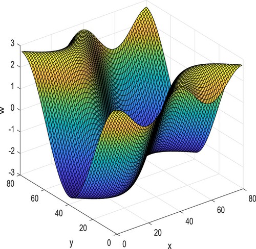
This sample explores finding the accurate solution for the given functions Comparisons between the accurate solution and the numerical solution are given in Tables 1 and 2 and Figures 2 and 3 when

Figure 2. The accurate and numerical solutions of . The exact solution is shown with dashes line.

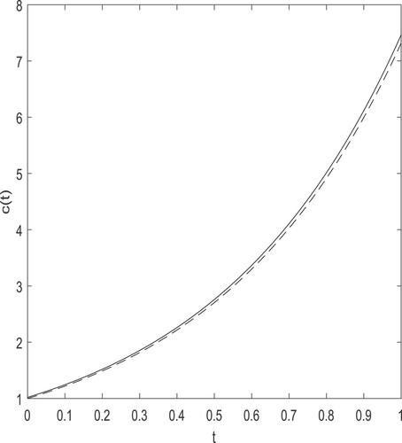
Figure 3. The numerical solution of .

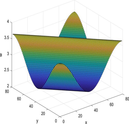
Table 1. The relative errors for the functions and in different step sizes.

Step sizes		Relative error for		Relative error for
σ	τ					Time in seconds
0.0393	0.005	0.02	0.0202	0.012	0.010	3.9
0.0393	0.01	0.04	0.0408	0.0121	0.0148	3.1
0.0196	0.01	0.013	0.0122	0.01	0.011	9
0.0196	0.005	0.018	0.0182	0.006	0.007	24.4

Table 2. The relative errors for the functions and in different expected tolerance.

Prescribed tolerance		Relative error in
for	for			CPU in sec.
		0.08	0.05	2.1
		0.02	0.01	3.9
		0.018	0.09	3.2
		0.004	0.005	38.4

According to Table 1, we choose the step sizes as , ,number of the grid points are Because CPU time is as important as relative error for the performance of the program

In this example for linearization iteration, the expected tolerance is and for predicting-correcting mechanism the prescribed tolerance is by using Table 2 considering CPU time and relative errors.

This programming has been performed using the MATLAB R2016 version of the computational program and CPU time is found using the tic-toc command in MATLAB.

Next, we will illustrate the stability of the numerical solution with respect to the noisy overdetermination data (5(5) ), defined by the function (34) where γ is the percentage of noise and ρ are random variables generated from a uniform distribution in the interval

In the case when T = 1, the illustrations of the sensitivity of the scheme with respect to noisy overdetermination data are shown in Table 3.

Table 3. The relative errors with some noisy data for the functions and in .

0% noisy data	0.02	0.01
1% noisy data	0.032	0.02
5% noisy data	0.058	0.081
10% noisy data	0.074	0.098

Example 4.2

This sample explores finding the accurate solution for the given functions In this example for linearization iteration, we choose the step sizes as , , the expected tolerance is and for predicting-correcting mechanism the prescribed tolerance is . Number of the grid points are

In the case when T = 1, the illustrations of the sensitivity of the scheme with respect to noisy overdetermination data are shown in Table 4.

Table 4. The relative errors with some noisy data for the functions and in .

0% noisy data	0.014	0.079
1% noisy data	0.021	0.092
5% noisy data	0.053	0.12
10% noisy data	0.081	0.18

In Examples 4.1 and 4.2 from Tables 3 and 4, it can be seen that the results are quite stable for small noise in the input data (Figures 4 and 5).

Figure 4. The accurate and numerical solutions of . The exact solution is shown with dashes line.

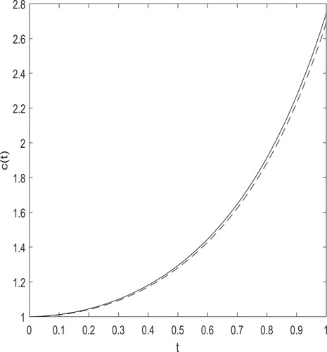
Figure 5. The numerical solution of .

5. Conclusion

The inverse problem of the temperature distribution in two-dimensional quasilinear parabolic equation by nonlocal conditions are taken. This inverse problem has been examined from both theoretically and numerically. In the theoretical part, the existence of the problem and the stability of the problem were examined. In the numerical process, finite difference method is used. Periodic boundary conditions are used in this article. Fourier method and the finite difference method are crucial of inverse problems for two-dimensional quasilinear parabolic equations.

In future studies, different conditions and different methods will be covered for two-dimensional problems. Also these methods can be considered different problems. Such problems can be resolved with different local or non-local boundary conditions. Also these problems can be examined with different methods like fractional method, operator method. According to literature on the numerical approximation of solutions of direct parabolic partial differential equations with standard condition many methods like finite difference, finite element, spectral, finite volume and boundary element methods have been proposed to approximate such solutions. In future these methods can be applied inverse parabolic problems with nonlocal boundary conditions [14,21–25].

Disclosure statement

No potential conflict of interest was reported by the author(s).

References

- Ramm AG. Inverse problems-mathematical and analytical techniques with application to engineering. New York: Springer; 2005.
- Sharma PR, Methi G. Solution of two dimensional parabolic equation subject to non-local conditions using homotopy perturbation method. J Appl Commun Sci. 2012;1:12–16.
- Ivanchov M, Vlasovi V. Inverse problem for a two-dimensional strongly degenerate heat equation. Electron J Differ Equ. 2018;77:1–17.
- Dehghan M. A new AD1 technique for two-dimensional parabolic equation with an integral condition. Pergamon Comput Math Appl. 2002;43:1477–1488.
- Dehghan M. A finite difference method for a non-local boundary value problem for two dimensional heat equation. Appl Math Comput. 2000;112:133–142.
- Afshar S, Soltanalizadeh B. Solution of the two dimensional second-order diffusion equation with nonlocal boundary condition. Int J Pure Appl Math. 2014;94(2):119–131.
- Gumel B, Ang WT, Twizellc EH. Efficient parallel algorithm for the two-dimensional diffusion equation subject to specification of massa. Int J Comput Math. 1997;64(1–2):153–163.
- Samaneh A, Soltanalizadeh B. Solution of the two-dimensional second-order diffusion equation with nonlocal boundary conditions. Int J Pure Appl Math. 2014;94(2):119–131.
- Dehghan M, Implicit solution of a two-dimensional parabolic inverse problem with temperature overspecification. J Comput Anal Appl. 2001;3(4):35–43.
- Kumar BVR, Priyadarshi G. Haar wavelet method for two-dimensional parabolic inverse problem with a control parameter. Rend Circ Mat Paler Ser 2. 2020;69:961–976.
- Mohebbi A. A numerical algorithm for determination of a control parameter in two-dimensional parabolic inverse problems. Acta Math Appl Sin. 2011;31(1):213–224. English Series.
- Li F, Wua Z, Ye C. A finite difference solution to a two-dimensional parabolic inverse problem. Appl Math Model. 2012;36:2303–2313.
- Dehghan M. Finite difference schemes for two-dimensional parabolic inverse problem with temperature overspecification. Int J Comput Math. 2000;75:339–349.
- Dehghan M. Identifying a control function in two dimensional parabolic inverse problems. Appl Math Comput. 2003;143(2):375–391.
- Meng Z, Zhao Z. Hermite spectral method for solving inverse heat source problems in multiple dimensions. Inverse Probl Sci Eng. 2017;25(9):1243–1258.
- Hill GW. On the part of the motion of the lunar perigee which is a function of the mean motions of the sun and moon. Acta Math. 1886;8:1–36.
- Baglan I, Kanca F. An inverse coefficient problem for a quasilinear parabolic equation with periodic boundary and integral overdetermination condition. Math Methods Appl Sci. 2015;38(530):851–867.
- Baglan I. Determination of a coefficient in a quasilinear parabolic equation with periodic boundary condition. Inverse Probl Sci Eng. 2015;23(5):884–900.
- Baglan I, Kanca F. Two-dimensional inverse quasilinear parabolic problem with periodic boundary condition. Appl Anal. 2019;98(8):1549–1565.
- Kanca F, Baglan I. Solution of the boundary-value problem of heat conduction with periodic boundary conditions. Ukr Math J. 2020;72(2):110–125.
- Ionkin NI, Solution of a boundary-value problem in heat conduction with a nonclassical boundary condition. Differ Equ. 1977;13:204–211.
- Feng P, Karimov ET. Inverse source problems for time-fractional mixed parabolic-hyperbolic-type equations. J Inverse Ill-Posed Probl. 2015;23(4):339–353.
- Atangana A, Mekkaoui T. Trinition the complex number with two imaginary parts: fractal fractal, chaos and fractional calculus. Chaos Solitons Fractals. 2019;128:366–381.
- Atangana A, Araz SI. Analysis of a new partial integro-differential equation with mixed fractional operators. Chaos Solitons Fractals. 2019;127:257–271.
- Atangana A, Sha A. Differential and integral operators with constant fractional order and variable fractional dimension. Chaos Solitons Fractals. 2019;127:226–243.