Inverse design of 3D curved ducts using a 3D-upgraded ball-spine algorithm

ABSTRACT

Achieving a unique solution for the 3D inverse design of a curved duct is a challenging problem in aerodynamic design. The centre-line curvature, and cross-sections’ area and shape of a 3D curved duct influence the wall pressure distribution. All the previous developments on the ball-spine method were limited to 2D and quasi-3D ducts, in which only the upper and lower lines of the symmetry plane were modified based on the target pressure distribution. In the present work, the ball-spine method was three-dimensionally developed for the design of curved ducts while considering the effects of cross-sectional shape and area. To validate the method, all the nodes of a 3D duct wall were iteratively corrected under the modified ball-spine method to reach the target geometry. The effects of the ball movement directions (spines) and the grid generation scheme in achieving the unique solution in inverse design were evaluated. The results showed that the new method converges to a unique solution only if the streamline-based grids are applied for the flow numerical solution, and the horizontal spines are considered as the directions for the displacement of the nodes. Finally, the wall pressure distribution of a high-deflected 3D S-shaped diffuser was three-dimensionally modified to reduce the separation, secondary flow, and flow distortion.

KEYWORDS:

• 3D-upgraded ball-spine method
• inverse design
• curved duct
• streamline-based grid generation
• secondary flow
• horizontal spines

1. Introduction

Intake is an important component of a propulsion system and directly affects the engine performance. Any separation or secondary flow inside the duct increases the total pressure losses and flow distortion at the engine inlet. The flow pattern in these ducts is quite complex as a result of both curvature and diffusion. This complication is also due to the presence of inflexion in the curvature.

Inverse design is an optimal shape design method that usually involves finding a shape associated with a prescribed distribution of surface pressure or velocity in fluid flow problems. However, the solution of an inverse shape design problem is generally not an optimum solution in a mathematical sense. This means that the solution only satisfies a target pressure distribution that resembles nearly optimum performance.

To solve inverse shape design problems, there are basically two different approaches: coupled (non-iterative) and decoupled (iterative) approaches. In a coupled approach, an alternative formulation of the problem is used in which the surface coordinates appear (explicitly or implicitly) as dependent variables. In other words, a fully coupled method reformulates the governing equations in a way that the shape, computational grid, and the fluid state are all updated simultaneously.

Stanitz [1–3] solved two- and three-dimensional potential flow duct design problems using stream and potential functions as independent variables. He reported the limitations of achieving a unique solution for the general 3D inverse problems [2,3]. Zannetti [4] developed a similar formulation for the Euler equations for the design of two-dimensional axisymmetric channels. Ahmed et al. [5] employed 2D boundary layer calculations combined with inviscid through-flow methods to predict the flow without swirl in axisymmetric diffusers. Chaviaropoulos et al. [6,7] formulated a fully coupled three-dimensional inverse design problem for the potential flow, and they required additional constraints to ensure uniqueness of the solution. Borges [8] transformed the variables from the physical plane (x–y) to a computational plane (ψ–ϕ) for the inverse design in 2D-irrotational incompressible flow.

Ashrafizadeh et al. proposed a direct inverse shape design method [9]. They showed that a fully coupled formulation of the inverse shape design problem could be solved in the physical domain using a simple extension of commonly used CFD algorithms. Raithby et al. [10] and Xuet al. [11] suggested the idea of providing a unified formulation for the solution of both analysis and design problems with one formulation for free surface turbulent flows. Taiebi-Rahni et al. [12] used the direct design approach for duct shape design with Euler equations. Ghadak [13] extended the application of this method for the design of ducts with non-linear coupled Euler equations.

The main difference of the coupled and decoupled algorithms is their shape modification strategy. In mathematically based decoupled inverse design algorithms, which are commonly called optimization methods, the difference between the target and current pressure distribution is defined as an objective function, and the minimum of this function is sought using ideas routed in calculus. In physically based decoupled inverse design algorithms, assumptions are made and physical analogies are employed to guide the shape evolution during the iterations.

Gradient-based optimization methods [14–16] generate and use information regarding the objective function gradients to specify the search direction and step size in the design space. Evolutionary methods [17–20] find the optimum solution based on repeated function evaluations. However, optimization methods are generally computationally expensive and mathematically complex. Nevertheless, they can be used to minimize the difference objective functions while satisfying the various constraints on the design variables. Wenbiao et al. [21] combines a robust optimization design and analysis of a conformal expansion nozzle of flying wing Unmanned Aerial Vehicle (UAV) with the inverse-design idea.

Physically based decoupled inverse design algorithms are rather mathematically simple, in which a linear relation is often established between the boundary node displacement $\left(\mathrm{\Delta }{r}_i\right)$ and the local surface pressure mismatch $\left(\mathrm{\Delta }{p}_i\right)$ to update the shape. Residual-correction methods were also developed to solve inverse shape design problems. Barger and Brooks [22] related the boundary curvature to the tangential velocity mismatch on the wall for an inviscid low. Garabedian and McFadden [23] proposed a residual-correction method called GM method to design a part of a transonic airfoil geometry. Malone et al. [24] developed a modified version of the GM method called MGM method to overcome some of the limitations. Dulikravich and Baker [25] proposed a method using elastic membranes, which considerably increased the convergence rate of the MGM method.

Nili-Ahmadabadi et al. [26] presented the flexile string algorithm as a residual-correction method for duct design, in which the duct wall was considered as a flexible string that deforms under the difference between the target and computed pressure distribution. The flexile string algorithm was developed for inviscid compressible [27] and viscous incompressible internal flow regimes [28]. Nili-Ahmadabadi et al. [29–32] developed another physics-based algorithm called the ball-spine method, in which the wall is considered as a set of separated balls that freely move along predefined directions called spines. Various alternatives of the ball-spine method have since been developed.

Vaghefiet al. [33] combined the ball-spine method and genetic algorithm for the shape optimization of diffusers without separation. Madadi et al. [34] developed the ball-spine method for the quasi-3D design of S-ducts with a predefined width distribution. Mayeli et al. [35,36] presented a novel way to make the ball-spine method capable of inverse shape design for conducting bodies with a desired heat flux distribution along the surface. Shumal et al. [37] used the ball-spine method for the swirling viscous flow regime to improve the performance of an axisymmetric duct with a 90-degree bend.

In the present work, the ball-spine method was three-dimensionally developed for the design of 3D S-shaped ducts with different cross-sectional shapes. The geometry correction method was validated by studying the effects of the movement direction (spine) of the balls and the grid generation method for different cross-sectional shapes in achieving a unique geometry. Three types of spines were studied for the validation: horizontal, vertical, and radial spines.

Two schemes of algebraic grid generation were also used for all the cross sections of the duct, in which the nodes of each cross section are calculated based on equally angled sectors or based on the streamlines lied on the wall. The wall nodes move along the specified spines to correct the geometry at each shape modification step. The results show that the 3D upgraded ball-spine method converges to a unique solution only if the streamline-based grids are applied for the flow numerical solution, and the horizontal spines are considered as the directions for the displacement of the nodes

Finally, the 3D design of an s-shaped diffuser with a height-to-axial-length ratio of 0.5 was performed to reduce the separation, secondary flow, and flow distortion inside the duct. The duct curvature was first obtained by a quasi-3D design of the duct’s symmetric plane using the optimal pressure distributions along the upper and lower lines. The pressure distributions along the critical cross sections with separation and secondary flow were modified to decrease the pressure gradients. The modified pressure distributions were applied three-dimensionally for the 3D inverse design of the duct.

2. Governing equations

2.1. Original 2D ball-spine equations

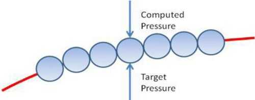
Figure 1 shows a 2D S-shaped duct with walls composed of a set of virtual balls that freely move along a specified direction called a spine. Fluid flow through the flexible duct causes a pressure distribution on the inner side of the wall. If a target pressure distribution is applied to the outer wall (Figure 2), the flexible wall deforms to reach a shape that satisfies the target pressure distribution. In other words, a force due to the difference between the target and current pressure distribution at each wall node is applied to each virtual ball, which starts moving. As the target shape is obtained, the pressure difference vanishes, and the balls stop moving.

Figure 1. Simulation of a 2D S-shaped duct with balls and spines.

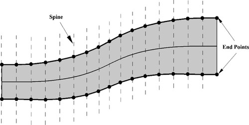
Figure 2. Applying the target and computed pressures on a sample ball.

In duct inverse design problems, a fixed characteristic length should be chosen to reach a unique inverse design solution. The direction of the spines should be defined based on the type of geometry. For a two-dimensional S-shaped duct, as shown in Figure 1, the spines are vertical lines normal to the x-coordinate, which causes the x-coordinate of the balls remain constant throughout the geometry correction process (Δx = 0). The constraint of Δx = 0 for the displacement of the balls leads to a fixed horizontal length of the S-shaped duct as the characteristic length during the geometry correction process.

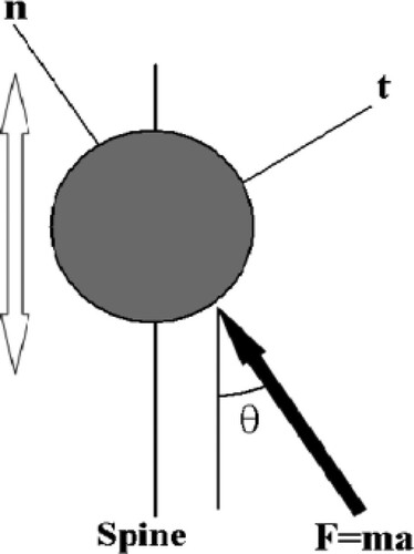
The kinematic relations of a flexible wall are derived by assuming a uniform mass distribution along the wall. The free-body diagram of a virtual ball on the wall is shown in Figure 3. The net force applied to the ball along the spine direction is computed as (1) $\begin{array}{rl}F& =\mathrm{\Delta }P\cdot A\cdot \text{cos}\theta \end{array}$(1) (2) $\begin{array}{rl}\mathrm{\Delta }P& =\left(P_{Target}-P_{Target\left(e\right)}\right)-\left(P_{Comp}-P_{Comp\left(e\right)}\right)\end{array}$(2) where the subscript e corresponds to the nodes on the outlet. According to Equation (2), $\mathrm{\Delta }P$ is gauged relative to the end ball on each wall to apply a zero force to the end balls on the outlet. The zero force at the outlet leads to a fixed outlet, which is another constraint to achieve a unique inverse design solution.

Figure 3. Free-body diagram of a sample ball on the duct wall.

If the ball moves along the spine through a specified time step $\left(\mathrm{\Delta }t\right)$, the corresponding displacement is computed from the following dynamic relations: (3) $\mathrm{\Delta }s=\frac{1}{2}a(\mathrm{\Delta }t{)}^2,a=\frac{F}{m}$(3)

Substituting Equations (1) and (2) into Equation (3) yields: (4) $\mathrm{\Delta }s=C\mathrm{\Delta }P\cos \theta$(4) where $C=A\cdot (\mathrm{\Delta }t{)}^2/2m$ is called the geometry correction coefficient and has the dimensions of $\left({\text{m}}^2\cdot {\text{s}}^2/\text{kg}\right)$. A large value of the parameter C increases the ball displacement and improves the convergence rate. However, if C exceeds a certain limit, the solution becomes unstable. Hence, an optimum value for the geometry correction factor should be determined through trial and error.

For the quasi-3D inverse design of an S-shaped duct, the symmetry plane of the S-shaped duct is considered as a 2D duct and the same original ball-spine equations are solved for the geometry correction process.

2.2. Three-dimensional upgraded ball-spine equations

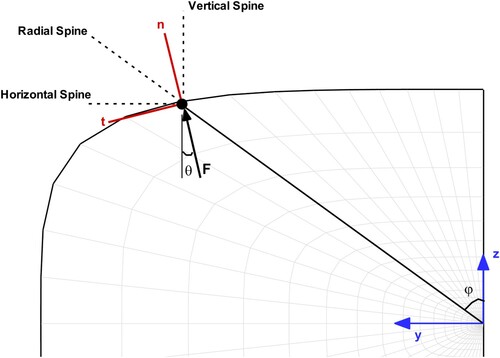
The direction of the spines in the inverse design of 2D ducts was vertical, while the direction of the spines for each cross-section in 3D ducts must be chosen so that they do not intersect during the inverse design process. So they can be considered vertical, horizontal, or radial, as shown in Figure 4. In addition, the cross-sections are perpendicular to the x-coordinate so that the direction of the spines does not interfere from one section to another. The effects of the spine direction on the uniqueness of the inverse design solution will be examined in Section 4.

Figure 4. Diagram of ball-spine direction in each cross section.

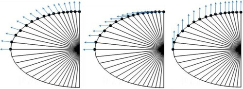
Figure 5 shows the schematic of force applied to the balls and the different spines for node displacement. For each cross-section, a local coordinate system is defined based on the centre-line of the diffuser. The force due to the pressure difference is applied perpendicular to the surface of the wall at each point while according to the direction of the spins, the balls are displaced according to the following equations: (5) $\begin{array}{c}Forverticalspine\\ \begin{array}{c}\downarrow \\ \begin{array}{c}{z}_i^{n+1}=z_i^n+C\cdot \mathrm{\Delta }{P}_i^n\cdot \cos \theta \\ y_i^{n+1}=y_i^n\\ x_i^{n+1}=x_i^n\end{array}\end{array}\end{array}$(5) (6) $\begin{array}{c}Forhorizontalspine\\ \begin{array}{c}\downarrow \\ \begin{array}{c}{y}_i^{n+1}=y_i^n+C\cdot \mathrm{\Delta }{P}_i^n\cdot \sin \theta \\ z_i^{n+1}=z_i^n\\ x_i^{n+1}=x_i^n\end{array}\end{array}\end{array}$(6) (7) $\begin{array}{c}Forradialspine\\ \begin{array}{c}\downarrow \\ \begin{array}{c}{y}_i^{n+1}=y_i^n+C\cdot \mathrm{\Delta }{P}_i^n\cdot \cos \left(\phi -\theta \right)\cdot \sin \phi \\ z_i^{n+1}=z_i^n+C\cdot \mathrm{\Delta }{P}_i^n\cdot \cos \left(\phi -\theta \right)\cdot \cos \phi \\ x_i^{n+1}=x_i^n\end{array}\end{array}\end{array}$(7) where i is the index for the node number and n is the index for the geometry correction number. The rest of parameters can be seen in Figure 5.

Figure 5. Schematic of force applied to the balls and the different spines for node displacement.

The inverse design of a 3D duct needs a new characteristic length in the cross sections to converge to a unique solution. As another constraint, the outlet area of the duct remains fixed throughout the shape-modification process because the gauged pressure at the outlet is zero (Equation (2)).

2.3. Calculating the grid points on the 3D wall surface

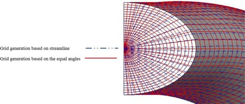
The location of the balls on each cross-section is an issue that must be considered in the 3D inverse design. That the grid points are or aren’t coincided with the locations of the balls during the geometry corrections can influence the convergence of the 3D inverse design procedure. Therefore, the grid generation scheme is important in the proposed inverse design method. The grid generation on each cross-section of the duct during the geometry corrections is accomplished based on the two following methods:

1. Grid generation based on equal angles between each two consecutive radial grid lines: Each cross section of the duct is divided into equal angles by radial grid lines. At each shape-modification step, the virtual balls at each wall node move along the specified spines. If the spine directions are vertical or horizontal, the angles between the consecutive radial grid lines will not be equal after each shape modification, so the grid must be regenerated based on the equal angles between each two consecutive radial grid lines. However, for the radial spines, the there is no need to regenerate this type of grid after each geometry correction.

2. Grid generation based on the streamlines lied on the wall: In a 2D duct inverse design, the lower and upper walls are two streamlines on which the virtual balls are placed and move along the spines. The virtual balls in a 3D duct inverse design should be placed on the lied streamlines on the wall to be similar to the 2D inverse design. After each shape modification, the wall nodes (virtual balls) are regenerated based on the calculated streamlines on the wall.

The velocity vector is defined as follows: (8) $\frac{\text{d}X}{\text{dt}}=\overrightarrow{V},X=\left(x,y,z\right),\overrightarrow{V}=\left(\overrightarrow{u},\overrightarrow{v},\overrightarrow{w}\right)$(8)

To draw the flow line, the following integral must be solved: (9) $X\left(t\right)=\underset{\tau }{\overset{}{\int }}\overrightarrow{V}\left(t\right)dt$(9)

The Runge–Kutta II method was applied as a numerical integration method to plot the flow line [38,39]. (10) $X_{i+1}=X_i+\left({\overrightarrow{V}}_i+{\overrightarrow{V}}_{i+1}\right)\mathrm{\Delta }t/\phantom{\mathrm{\Delta }t2}2,X_{i+1}=X_i+{\overrightarrow{V}}_i\mathrm{\Delta }t$(10)

In these equations, t is an independent parameter, and the velocity vector and the coordinates of the wall nodes are dependent on it. The coordinates x, y, and z are separately obtained for each deterministic Δt. The grid generation of the geometry is carried out in a way that the cross sections are placed at distinct x-positions in the horizontal direction, so the wall grid nodes are calculated on the streamlines lied on the wall as follows: (11) $\begin{array}{rl}\frac{dx}{dy}& =\frac{du}{dv},\frac{dx}{dz}=\frac{du}{dw}\\ y_{i+1}& =y_i+{\int }_i^{i+1}\frac{v}{u}dx,z_{i+1}=z_i+{\int }_i^{i+1}\frac{w}{u}dx\end{array}$(11)

The y- and z-coordinates of the wall grid nodes on the corresponding streamlines are obtained for equal horizontal distances$\left(\mathrm{\Delta }x\right)$ between the cross sections. (12) $\begin{array}{rl}{y}_{i+1}& =y_i+\left(\frac{v_i}{u_i}+\frac{v_{i+1}}{u_{i+1}}\right)\mathrm{\Delta }x/\phantom{\mathrm{\Delta }x2}2\end{array}$(12) (13) $\begin{array}{rl}{z}_{i+1}& =z_i+\left(\frac{w_i}{u_i}+\frac{w_{i+1}}{u_{i+1}}\right)\mathrm{\Delta }x/\phantom{\mathrm{\Delta }x2}2\end{array}$(13)

To draw the streamlines and calculate the grid nodes on the wall, the duct’s outlet section is considered fixed, and the wall nodes along the streamlines are calculated by space marching from the end to the beginning of the duct using the Runge–Kutta-II method. Figure 6 clearly shows that the two types of grid generation methods for an S-duct geometry are not coincided with each other.

Figure 6. Diagram of geometry with two methods for grid generation.

After each shape modification, the process of flow solution and grid generation should be carried out iteratively to calculate the wall pressure distribution along the grid lines on the wall. After updating the grid nodes on the duct wall, new grids are generated for the internal domain, and the flow equations for the new grids are solved to compute the new wall pressure distribution. The procedure is repeated until the pressure distributions match.

These two methods of grid generation are examined for all cross-sections to evaluate the appropriate positions of the control points on the wall during the inverse design procedure.

2.4. Wall smoothing operation

Since the wall is considered as a set of separate virtual balls, the wall curvature may be discontinuous because the wall may become zigzag during the geometry correction process. To smooth the wall curvature, a Savitzky–Golay filter [40,41] is applied to the wall nodes after each geometry correction step. The Savitzky–Golay filter method performs a local polynomial regression to determine the smoothed values for each data point. In this paper, the filtration was performed using a second-order polynomial with 5 data points. The equation for this particular Savitzky–Golay smoothing is defined as follows: (14) $g_i=1/35\left(\sum _{n=n_L}^{n_R}{C}_n{f}_{n+i}\right)$(14) where $g_i$ is the filtered value at the position i, $f_j$ is the unfiltered value at the position j, $n_L$ and $n_R$ respectively specify the data points on the left and right of the point that are supposed to be smoothed, and $C_n$ is the weighting function according to Table 1.

Table 1. Weighting function for SG using second-order polynomial and 5 data points.

	$n_L$	$n_R$	n = −4	n = −3	n = −2	n = −1	n = 0	n = 1	n = 2	n = 3	n = 4
For the beginning points	0	4	–	–	–	–	31	9	−3	−5	3
	1	3	–	–	–	9	13	12	6	−5	–
For the middle points	2	2	–	–	−3	12	17	12	−3	–	–
For the end points	3	1	–	−5	6	12	13	9	–	–	–
	4	0	3	−5	−3	9	31	–	–	–	–

Table 1 shows the weighting function for Savitzky–Golay smoothing scheme using second-order polynomial and five data points. Because the wall geometry is a three-dimensional shell, the filtering is carried out at the intersection of each longitudinal section and each cross-section by means of the nine points shown in Figure 7.

Figure 7. Schematic of points used for filtration along the longitudinal and cross-sections.

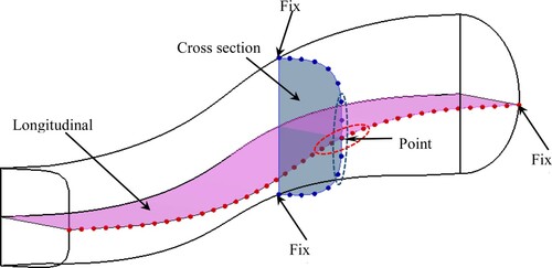
According to Figure 7, the filtration is performed for all points of the longitudinal sections (red points) based on Equation (14). Due to the specific section at the outlet, the end point of each longitudinal section is fixed. Filtration is also performed at each cross-section (blue points) and the upper and lower points of each cross-section on the symmetry plane are kept constant in order to fix the duct centreline.

2.5. Euler equations

An Euler solver was coupled with the inverse design algorithm to calculate the wall pressure distribution at each geometry correction. The governing equations of the Euler solver for three-dimensional, compressible, and inviscid flow in the conservative form are as follow: (15) $\frac{\mathrm{\partial }Q}{\mathrm{\partial }t}+\frac{\mathrm{\partial }E}{\mathrm{\partial }x}+\frac{\mathrm{\partial }F}{\mathrm{\partial }y}+\frac{\mathrm{\partial }G}{\mathrm{\partial }z}=0$(15) where (16) $\begin{array}{r}Q=\left[\begin{array}{c}\rho \\ \rho u\\ \begin{array}{c}\rho v\\ \begin{array}{c}\rho w\\ \rho e_t\end{array}\end{array}\end{array}\right],E=\left[\begin{array}{c}\rho u\\ \rho u^2+P\\ \begin{array}{c}\rho uv\\ \begin{array}{c}\rho uw\\ \rho uH\end{array}\end{array}\end{array}\right],F=\left[\begin{array}{c}\rho v\\ \rho vu\\ \begin{array}{c}\rho v^2+P\\ \begin{array}{c}\rho vw\\ \rho vH\end{array}\end{array}\end{array}\right],G=\left[\begin{array}{c}\rho w\\ \rho wu\\ \begin{array}{c}\rho wv\\ \begin{array}{c}\rho w^2+P\\ \rho wH\end{array}\end{array}\end{array}\right]\end{array}$(16) where Q is the conservative vector, and E, F and G are the inviscid flux vectors. ρ is the fluid density, P is the pressure, H is the enthalpy, and u, v, and w are the velocity components. To solve the inviscid flow equations through a 3D domain, an in-house code based on Advection Upstream Splitting Method (AUSM) [42] scheme was used. AUSM was developed as a numerical inviscid flux function for solving a general system of conservation equations.

For compressible flow in a diffuser, the total pressure at the inlet and static pressure at the outlet were applied as the boundary conditions. Zero flux was applied to the diffuser wall and the symmetry boundary condition was applied to the symmetry plane.

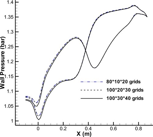
The pressure distribution at each geometry correction was obtained by an Euler inviscid solver that is not highly sensitive to the grid refinement. However, the appropriate grid size should be evaluated before starting an inverse design. To do this, the wall pressure distribution should be first calculated by different grid sizes and then compared to each other. The grid size was optimized through a grid refinement study. In this respect, the computational domain was meshed by O-grid structured mesh with $N_x\times N_r\times N_{\theta }=80\times 10\times 30,100\times 20\times 30,\text{and}100\times 30\times 40$. $N_x,N_r$ and $N_{\theta }$ imply the number of nodes in the axial, radial and angular directions, respectively. The wall pressure distribution along the upper and lower lines of the symmetry plane was obtained for various grid sizes and plotted in Figure 8. It is apparent that for grid sizes finer than $N_x\times N_r\times N_{\theta }=100\times 20\times 30$, the results are identical.

Figure 8. Grid-independency for wall pressure distribution along the upper and lower lines of the symmetric plane.

3. Inverse design procedure

As mentioned before, the cross-sections’ area and profile as well as the duct curvature affect the pressure contour and flow quality of a 3D curved duct. Therefore, the three-dimensional inverse design is carried out in two steps so that in each step only one of them affects the pressure contour. At the first step, the width of each cross-section changes in a way that the cross-section area is fixed to remove the effect of area on the pressure contour, and only the symmetry plane of the duct is corrected using the optimal pressure distributions along the upper and lower lines [34]. In other words, a quasi-3D inverse design is performing at the first step to achieve the duct curvature. In the second step, all cross-sections are corrected through a three-dimensional inverse design with a constant curvature. All the wall nodes except the nodes on the upper and lower lines of the symmetry plane can be displaced by applying the force due to the pressure difference. In other words, the centre-line of the duct is also kept constant and the wall nodes are allowed to be displaced along the selected spines for all cross-sections (vertical, horizontal or radial). By doing these two steps, all the wall nodes can be controlled by the three-dimensional inverse design procedure.

3.1. Quasi-3D inverse design for the symmetry plane

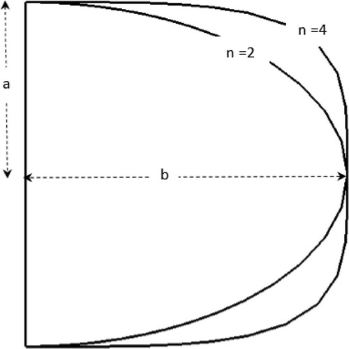
If a super ellipse according to Equation (17) is used for drawing the cross-sections of an S-shaped duct, the profile of all cross-sections is controlled by the parameters a, b, and n, as shown in Figure 9. (17) $\frac{y^n}{b^n}+\frac{z^n}{a^n}=1$(17)

Figure 9. Diagram of cross-sectional design parameters.

In the quasi-3D design of the S-shaped duct, which was performed by Madadi et al. [34], the cross-sectional profile of the initial guess was known and equal to that of the target geometry. In other words, the parameters b and n were known and only the parameter a should be obtained based on the geometry corrections on the symmetric plane. The first step of the design procedure in the current work is not the same as performed by Madadi et al. [34] because the cross-sectional profiles in the initial geometry are not known and can be different from those in the target geometry. Therefore, in the first step of the design procedure, the effect of cross-sectional profile on the pressure distribution along the upper and lower lines of the symmetry plane should be eliminated to achieve the duct curvature. To do this, the width of the cross-sections changes at each correction of the symmetry plane according to Equation (18) so that the mean pressure of each cross-section is the same as the mean pressure in the target geometry. (18) $b_{new}=b_{old}\left(P_{Ave,Target}/P_{Ave,Current}\right)$(18)

In Equation (18), $P_{Ave}$ is the average pressure of each cross-section, and $b_{old}$ and $b_{new}$ are respectively the current and the modified width of each cross-section.

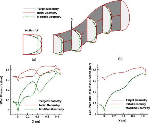
Figure 10 shows three geometries with the same symmetry plane and different cross-sections. The pressure distributions along the upper and lower lines of the symmetry plane and the mean pressure distributions versus x are also shown in Figure 10 for all three geometries. There is a big difference between the pressure distribution along the upper and lower lines of the symmetry plane for the initial and target geometry due to the difference between their cross-sectional areas. To remove the effect of cross-sectional area, the width of each cross-section is modified according to Equation (18) so that each cross-sectional area of the modified geometry becomes equal to that of the target geometry. It causes the pressure distributions along the upper and lower lines of the symmetry plane to be almost the same for the modified and target geometries despite the different cross-sectional profiles, as shown in Figure 10. Moreover, the mean pressure distributions along the centrelines of the modified and target geometry become equal.

Figure 10. Three geometries with the same centre-line curvature and different cross-sections, and (a) their corresponding pressure distributions along the upper and lower lines of the symmetry plane, and (b) average pressure of cross-section.

For validation of the first step of the inverse design method, an arbitrary S-shaped diffuser is chosen as the target geometry, and the pressure distribution along the upper and lower lines of the symmetry plane is considered as the target pressure distribution. Then, a straight diffuser with different cross-sections is considered as the initial guess geometry for the inverse design problem. If the final symmetry plane reaches the target symmetry plane through the geometry correction process, the first step of the inverse design procedure can be validated.

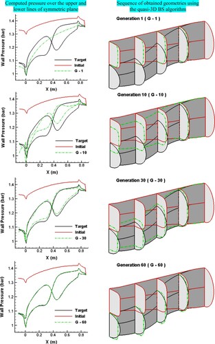
Figure 11 shows the first step of geometry correction procedure and pressure contour for the initial guess with n = 6 while the cross-sectional profile of the target geometry is different (n = 2). In the first generation (G – 1), the width of each cross-section is modified so that the average pressure of each cross-section is the same as that for the target geometry. During each correction of the symmetry plane, the width of the cross-sections is recalculated to control the average pressure. Finally, the duct symmetry plane reaches the target while the cross-sectional profiles can be different for the final and target geometries.

Figure 11. Evolution of geometries and their corresponding pressure distributions from the initial guess to the target geometry.

3.2. Three-dimensional inverse design for modifying the cross-sectional profiles

A three-dimensional upgraded ball-spine approach was proposed to correct the duct’s lateral lines and cross sections. In the previous step, the duct curvature was obtained from a quasi-3D inverse design. With a fixed centre-line for the duct, the ball-spine method was applied three-dimensionally to all lines on the wall to converge to a target geometry that satisfies the target pressure distribution on all the nodes of the duct wall. In other words, during the three-dimensional inverse design procedure, the profile of each cross-section is obtained based on the nodes displacements in Equations (5)–(7), and the defined cross-sectional profile in Equation (17) is used only for the initial and target geometry.

The inviscid flow equations are solved using the AUSM scheme to compute the current pressure distribution on the duct wall. The difference between the target and current pressure distributions along all the lines lied on the wall causes all the wall nodes to be corrected. According to the selected spine (vertical, horizontal or radial), the new position of the wall nodes is obtained based on the Equations (5)–(7). For vertical or horizontal spines, which are shown in Figure 9, a or b remains constant so that the constraint of a fixed characteristic length is automatically satisfied through the inverse design process.

The 3D geometry of the S-duct is regenerated using the updated wall and the fixed centre-line. Each cross-section of the new geometry is remeshed by one of the two grid generation schemes. The two grid generation schemes should be examined to select the appropriate control points on the duct wall at each cross-section. The grid generation and flow solution are then accomplished to calculate the current pressure distributions on all wall nodes. The procedure is repeated until the current and target pressure distribution along all lines on the wall match.

4. Validation and conditions for unique solution in 3D inverse design

To validate an inverse design method, a target geometry is assumed, and the corresponding wall pressure distribution is considered as the target pressure (Figure 12). If an arbitrary geometry as an initial guess converges to the target geometry through the inverse design procedure, the inverse design method has been validated. The results of the geometry correction process for different initial geometries are shown below to verify the necessary conditions of the numerical scheme to reach a unique solution. For other figures, the pressure contour results are shown only for the lines φ = 0.90,180 (Figure 12).

Figure 12. Target geometry and corresponding wall pressure distribution.

4.1. Grid generation based on equal angles between consecutive radial grid lines

Grid generation for the duct was first carried out based on equal angles between consecutive radial grid lines. The uniqueness of the inverse design solution was then studied for the radial, vertical, and horizontal spine directions.

1. Radial spines

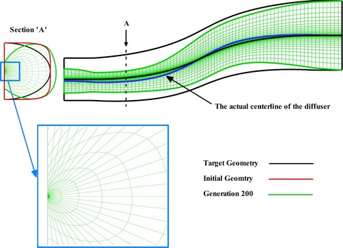
For the radial spines, the final geometry does not exactly converge to the target geometry in spite of using the same profiles for the initial guess and target geometry, while the final pressure distribution converged to the TPD, as shown in Figures 13 and 14. This is due to the width and the height of the cross sections not being fixed throughout the geometry correction for the radial spines. The inverse design diverges if the cross-sectional profiles for the initial guess and target geometry are not similar, as shown in Figure 15. In Figure 15, the pressure difference on the symmetric plane between the target and initial geometry is only due to the difference in the cross-sections’ area and profile. To study the effects of the cross-sections’ area and profile on the pressure contour, it is necessary to keep the centreline constant. The use of radial spins causes this pressure difference to move the wall lines of the symmetric plane, and change the actual curvature of the centreline as well as the cross-sections’ area and profile, while the grid generation is based on a constant centreline. A simultaneous change in the actual curvature, and cross-sections’ area and profile confuses the geometry correction scheme to use the pressure difference for wall nodes displacement, which diverges the inverse design. Figure 16 shows that the inverse design process diverges after 200 geometry corrections when the different cross-sectional profiles are used for the initial and target geometry. The deformed mesh is also shown on the symmetric plane and cross section ‘A’, which clearly indicates the solution divergence as the walls approach the centreline.

1. Vertical spines

Figure 13. Results of inverse design with similar cross-sectional profiles (n = 2) for the initial and target geometry using an equally angled grid and radial spines after 150 geometry corrections.

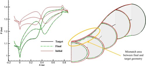
Figure 14. Results of inverse design with similar cross-sectional profiles (n = 4) for the initial and target geometries using an equally angled grid and radial spines after 150 geometry corrections.

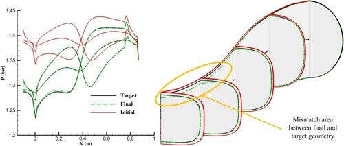
Figure 15. Results of inverse design with different cross-sectional profiles for the initial guess (n = 6) and target geometries (n = 2) using an equally angled grid and radial spines after 150 geometry corrections.

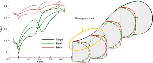
Figure 16. Results of inverse design with different cross-sectional profiles for the initial guess (n = 6) and target geometries (n = 2) using radial spines after 200 geometry corrections.

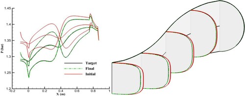
Figures 16 and 17 show that the 3D upgraded ball-spine method was validated for the vertical spines when the cross-sectional profiles for the initial guess and target geometry were similar with the same parameter n in Equation (17). The cross-sectional profiles in Figure 17 are elliptical (n = 2), while in Figure 18, they are all semi-elliptical (n = 4). Similar to the results of the radial spines, the inverse design with the vertical spines diverges if the cross-sectional profiles of the initial guess geometry are different from that of the target geometry (Figure 19).

Figure 17. Results of inverse design with similar cross-sectional profiles (n = 2) for the initial and target geometries using an equally angled grid and vertical spines after 200 geometry corrections.

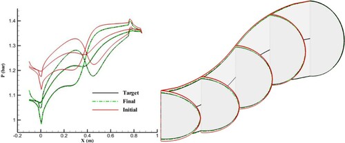
Figure 18. Results of inverse design with similar cross-sectional profiles (n = 4) for the initial and target geometries using an equally angled grid and vertical spines after 200 geometry corrections.

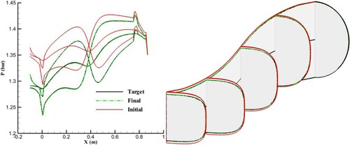
Figure 19. Results of inverse design with different cross-sectional profiles for the initial guess (n = 6) and target geometry (n = 2) using an equally angled grid and vertical spines after 200 geometry corrections.

With the vertical spines, when the cross-sectional profiles are similar for the initial guess and target geometry, the change in the pressure distribution for all the wall lines is only due to the change in the cross-sectional area or the height of each cross section, so only the parameter a changes during the geometry correction process, and the inverse design process converges. In other words, when the parameters b and n are fixed during the geometry corrections, convergence occurs. However, for different cross-sectional profiles with vertical spines, both a and n change during the geometry correction process and significantly influence the wall pressure distribution. The duct’s centre line is significantly displaced, and the inverse design process diverges.

1. Horizontal spines

Similar to the results of vertical spines, the inverse design with horizontal spines converges if the type of cross-sectional profile is the same for the initial guess and target geometry, as shown in Figures 20 and 21. For these conditions, a and n are automatically fixed, and only b changes.

Figure 20. Results of inverse design with similar cross-sectional profiles (n = 2) for the initial and target geometries using an equally angled grid and horizontal spines after 200 geometry corrections.

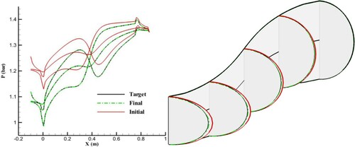
Figure 21. Results of inverse design with similar cross-sectional profiles (n = 4) for the initial and target geometries using an equally angled grid and horizontal spines after 200 geometry corrections.

As indicated for vertical and radial spines, the inverse design diverges if only one parameter is fixed during the geometry corrections. Only a remains fixed during the geometry corrections when the cross-sectional profiles for the initial guess and target geometry are different and horizontal spines are used for the wall node displacement. Therefore, divergence is expected.

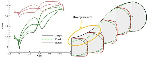
Figure 22 shows the results of the inverse design with different cross-sectional profiles for the initial guess (n = 6) and target geometry (n = 2) with horizontal spines. Although the final pressure distribution converged to the TPD, the final geometry is different from the target geometry. In other words, there is no unique solution for this inverse design. However, the final geometry has the same cross-sectional profile as the initial geometry. Nevertheless, the pressure distributions converge to the TPDs on all wall nodes due to the fixed symmetry plane for this inverse design. At the next section, the streamline-based grids will be used for the horizontal spine to reach a unique solution.

Figure 22. Results of inverse design with different cross-sectional profiles for the initial guess (n = 6) and target geometry (n = 2) using an equally angled grid and horizontal spines.

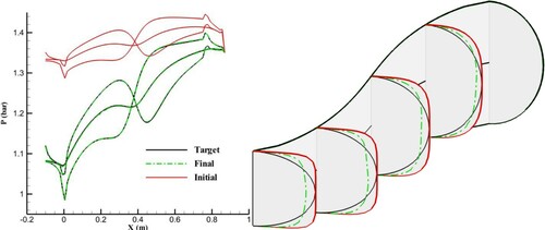
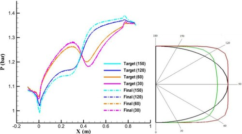
Figure 23 shows that the final pressure distributions along the wall lines at various sectors with angles of 30, 60, 120, and 150 degrees converged to the corresponding TPDs, while the final cross section is different from the target cross section.

Figure 23. Comparison of wall pressure distributions for the target and final geometry with an equally angled grid along the lateral lines of the wall at various sectors.

4.2. Streamline-based grid generation with horizontal spines

Equally angled radial grid lines led to non-uniqueness of the 3D inverse design, so 2D and 3D inverse designs were compared to resolve this problem. In a 2D inverse duct design, the duct’s upper and lower lines are considered as the two streamlines, but in a 3D inverse design with an equally angled grid generation scheme, the wall lines are not exactly the streamlines. This difference leads to a failure to reach a unique solution. Therefore, at each geometry correction step, the grid generation should be based on the streamlines on the wall so that the wall nodes correspond to the wall streamlines. Thus, the current and target pressure distributions were compared along the corresponding streamlines on the existing wall and target duct wall.

Figures 24 and 25 show the streamline-based grids for the initial guess and target geometry with the same and different cross-sectional profiles, respectively. When the initial guess and target geometry have the same cross-sectional profile (Figure 24), the wall streamlines are close to the wall lines obtained from the equally angled sectors, so the type of grid generation does not affect the uniqueness of the solution. However, for the different cross-sectional profiles (Figure 25), the wall streamlines are very far from the equally angled sector wall lines, which causes a non-unique solution.

Figure 24. Comparison of streamline-based and equally angled grid generation for the initial guess and target geometry with the same cross-sectional profile.

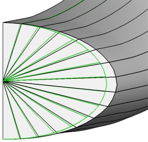
Figure 25. Comparison of equally angled (a) and streamline-based (b) grid generation for the initial guess and target geometry with different cross-sectional profiles.

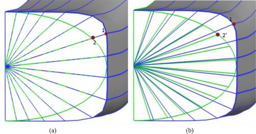
Therefore, the current and target pressure distributions should be compared at the corresponding nodes obtained from the streamline-based grid generation to reach a unique solution. When the equally angled grid generation is used, a wrong comparison is carried out between the corresponding nodes, leading to a non-unique solution. According to Figure 24, for the equally angled grid generation, points 1 and 2 are the corresponding nodes at the initial guess and target geometry, while for the streamline-based grid generation, points 1 and 2’ are the corresponding nodes.

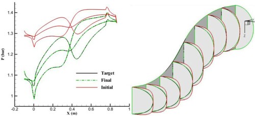
The final and target geometries shown in Figure 22 were remeshed based on the wall streamlines. The pressure distributions along the corresponding wall streamlines for the final and target geometries are compared in Figure 26. A comparison between Figures 23 and 26 indicates that the wall pressure distributions of the final and target geometries do not match for the streamline-based grid, while they do match for the equally angled grid. The streamline-based grid shows wall pressure differences for the final and target geometries, but the equally angled grid does not. Therefore, the streamline-based grid is expected to be capable of resolving the non-uniqueness problem. To prove this, an inverse design with the streamline-based grid and horizontal spines was performed using a target geometry with an elliptical cross section (n = 2) and an initial guess with a super-ellipse cross section (n = 4). Figure 27 shows the results, which indicate convergence to a unique solution.

Figure 26. Comparison of wall pressure distributions for the target and final geometry with streamline-based grid along the wall streamlines

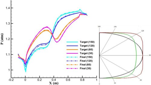
Figure 27. Results of inverse design with different cross-sectional profiles for the initial guess (n = 4) and target geometry (n = 2) using the streamline-based grid and horizontal spines after 200 corrections.

4.3. Summarizing the validation cases and unique solution conditions

Inverse design methods have a series of limitations to achieve unique solution, and they are ill-posed for some conditions. These limitations are different due to differences in the type of methods (coupled or decoupled) or differences in the numerical techniques. Some previous researches reported the limitations of achieving a unique solution for the general 3D inverse problems. Stanitz [2,3] reported that when he used the upstream boundary shape and the lateral velocity distribution on the duct wall as the inputs for a coupled 3D inverse design, the boundary conditions were overprescribed and the problem was ill-posed. He proposed degrees of compatibility between the inputs to achieve satisfactory solutions. Chaviaropoulos et al. [6,7] investigated the existence and uniqueness of the solution for 3D potential inverse design of ducts with target pressure. They indicated the inverse problem to be ill-posed with multiple solutions. They alleviated this multiplicity by considering stream-tubes with orthogonal cross-sections. They also reported some limitations in defining the ducts for the 3D inverse design.

As mentioned before, the fixed characteristic length and fixed outlet were required for the 2D and quasi-3D ball-spine method to converge a unique solution. However, there are some more limitations for 3D upgraded ball-spine method to achieve unique solution. In the current research, the constraints for resolving these limitations were proposed and evaluated. Table 2 summarizes the conditions for the convergence and uniqueness of inverse design solution. The parameters a and b are the height and width of the diffuser sections, respectively, according to Figure 10. The parameter n indicates the type of profile for the cross-sections of the initial geometry.

Table 2. Conditions for convergence and unique solution for the inverse design of the s-shape diffuser.

			N
Parameters	a	b	Similar to the target	Arbitrary
Radial spines	Not fixed	Not fixed	Converged but not unique	Diverged
Vertical spines	Not fixed	Automatically fixed	Converged and unique	Diverged
Horizontal spines	Automatically fixed	Not fixed	Converged and unique	Converged but unique only for streamline-based grid

For 3D upgraded ball-spine method, one of the cross-section parameters (a or b) additional to the duct length is required to be fixed as the cross-section characteristic length to achieve a unique inverse solution. Because both a and b are not fixed for the radial spines, the answer is not unique. For the horizontal and vertical spines, if the cross-sectional profile of the initial geometry is similar to the target, the pressure difference is only due to the difference in area, and the unique answer can be reached. If the cross-sectional profile of the initial geometry is not the same as the target, the difference in profile and area will cause a pressure difference on the diffuser symmetric plane. In vertical spines, this pressure difference changes the actual centreline of the diffuser, and the effects of its curvature on the pressure contour are included, which causes the inverse design to diverge. In horizontal spines, the diffuser symmetric plane and centreline are fixed, and only the cross-sections’ area and profile affect the pressure contour, which causes the inverse design to converge. However, the answer is not unique for different cross-sectional profiles of the initial and target geometry, because the scattering of the cross-sectional streamlines in the current geometry differs from those in the target geometry. If the grid generation is based on the wall streamlines, the corresponding nodes on the current and target wall geometry are correctly selected for comparing their pressure, which causes a unique inverse solution.

5. Design example

In order to show the capability of the 3D inverse design method, the wall pressure distribution of a high-deflected 3D S-shaped diffuser with a fixed centre line was modified, and then applied to the three-dimensional ball-spine method to increase the efficiency and to reduce flow distortion and separation inside the duct.

First, the upper and lower line of an S-shaped diffuser are modified via the quasi-3D inverse design on the symmetry plane according to an optimum pressure distribution along the upper and lower lines [34].

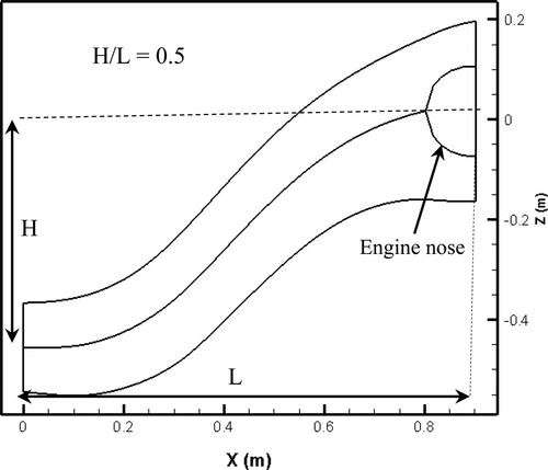
In the quasi-3D inverse design, the height-to-axial-length ratio of the duct is 0.5, and the cross-sectional profile is considered elliptical with a constant width. The inlet and outlet Mach numbers are 0.7 and 0.4, respectively. To demonstrate the design capability and take into account the actual operating conditions of the diffuser, the engine nose is also modeled at the duct outlet. In fact, by adding a nose, which is a part of the engine located at the end of the diffuser, its effects on the performance of the duct and the current distortion are considered, and in addition to shortening the diffuser, the design is closer to the real situation.

The pressure distributions were chosen so that separation would not occur in the symmetry plane of the duct. Figure 28 shows the optimum pressure distribution of the upper and lower lines of the symmetry plane. Figure 29 also shows the symmetry plane of the quasi-3D designed S-duct based on the optimum pressure distribution.

Figure 28. Optimum pressure distribution along the upper and lower lines of the symmetry plane of an S-duct as a TPD for quasi-3D inverse design.

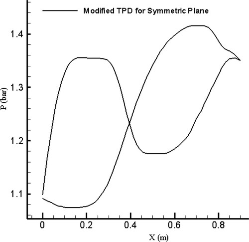
Figure 29. Symmetric plane of the quasi-3D designed S-duct corresponding to the optimum pressure distribution.

A RANS flow solver with an SST turbulence model numerically solved the flow equations to obtain the flow field inside the quasi-3D designed S-duct. As expected, there was no separation through the symmetry plane of the quasi-3D designed duct, as shown in Figure 30. This is due to the symmetry plane being designed according to the optimum pressure distribution along the upper and lower lines. According to Figure 31, the 3D streamlines clearly show the occurrence of secondary flow on the upper wall of the quasi-3D designed S-duct.

Figure 30. Streamlines through the symmetry plane of the quasi-3D designed S-duct.

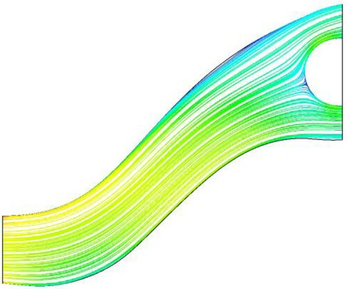
Figure 31. 3D streamlines on the upper wall of the quasi-3D designed S-duct.

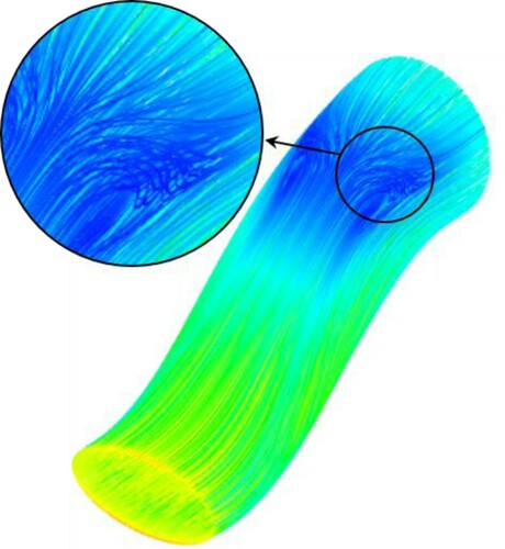
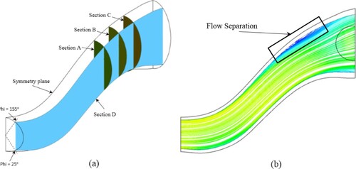
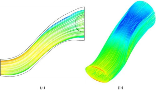
Although there is no separation on the symmetry plane, a separation occurs through the adjacent planes of the symmetry plane (Figure 32(b)) due to the secondary flow, as shown in Figure 31. The visualized separation in Figure 30(b) cannot be controlled by the quasi-3D inverse design. Therefore, a full-3D inverse design is necessary to remove the separation and secondary flow inside the S-duct, which was designed via the quasi-3D inverse design.

Figure 32. Streamlines and flow separation corresponding to the plane adjacent to the symmetry plane (section D) for the quasi-3D designed S-duct.

For a full-3D aerodynamic design of the S-duct in Figure 31, the wall pressure contour should be modified and applied to the 3D ball-spine inverse design method to automatically correct the cross-sectional profiles of the duct. The 3D inverse design was carried out according to the streamline-based grid and horizontal spines with a fixed symmetry plane. The wall pressure contours through the region of the secondary flow were modified so that the pressure gradients along the cross sections would decrease, and the pressure changes from the top to the bottom would be smooth.

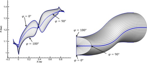
Figure 33 shows the modified pressure distributions of sections A, B, and C as examples. Figure 34 shows the original and modified pressure distributions of the upper and lower lines of section D in Figure 32(a). Figure 33 compares the three-dimensionally designed S-duct based on the modified pressure contour with the quasi-three-dimensionally designed S-duct. According to the figure, the cross sections through the secondary flow in Figure 35 were corrected by the 3D ball-spine inverse design. Figure 36 illustrates the 2D streamlines inside section D and the 3D streamlines inside the entire duct. It is clear that the separation and secondary flow have been eliminated from the new duct.

Figure 33. Modification of the wall pressure distribution along the cross sections.

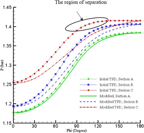
Figure 34. Modified pressure distribution of the upper and lower lines of section D.

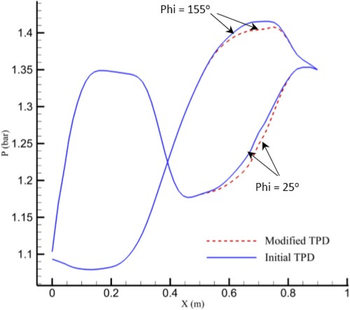
Figure 35. Comparison of the quasi-3D design with the 3D designed S-duct.

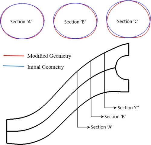
Figure 36. 2D streamlines of section D (a) and 3D streamlines (b) inside the 3D designed S-duct.

Figure 32 Streamlines and flow separation corresponding to the plane adjacent to the symmetry plane (section D) for the quasi-3D designed S-duct.

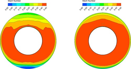
Figure 37 illustrates the Mach number contours at the outlet of the quasi-3D and 3D designed S-ducts. The uniformity of the Mach number distribution strongly affects the engine performance. It is clear that the outlet Mach number of the 3D designed S-duct is more uniform than the quasi-3D designed one. This is the result of modifying the pressure contours on the planes adjacent to the symmetry plane and eliminating the separation and secondary flow inside the duct.

Figure 37. Mach number contours at the outlet of the quasi-3D and 3D designed S-ducts.

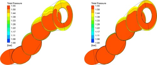
In Figure 38, the total pressure contours for different cross sections are compared for the quasi-3D and 3D designed S-ducts. The total pressure loss was decreased through the 3D designed S-duct due to the modified cross-sectional profiles obtained by 3D inverse design.

Figure 38. Contours of stagnation pressure in various axial positions for the quasi-3D and 3D designed S-ducts.

The uniformity of total pressure distribution at the engine face is an important parameter in relation to compressor efficiency and stability. An expression for a distortion coefficient to quantitatively measure the flow irregularities or total pressure distortion at the engine face is DC (90) defined as (17) $DC\left(90\right)=\frac{Max|P_{0,ave}-P_{0,ave,90}|}{1l2\rho U^2}$(17) where $P_{0,ave}$ is the average total pressure at the duct outlet and $P_{0,ave,90}$ is the average total pressure over a 90 deg sector of the engine face. For the 3D designed S-duct, DC (90) is equal to 0.019.

Table 3 compares the performance of the 3D designed S-duct with that of the quasi-3D designed case. As seen, the 3D designed S-duct has a more uniform flow at the engine inlet and its DC (90) is significantly lower. In addition, it has a lower pressure loss and a higher pressure recovery.

Table 3. Comparison between quasi-3D designed S-duct performance and 3D designed.

Parameter	Quasi-3D designed	3D designed
$DC\left(90\right)=\frac{Max\left|P_{0,ave}-P_{0,ave,90}\right|}{1l2\rho U^2}$	0.041	0.019
Pressure recovery coefficient $CPR=\frac{P_2-P_1}{P_{01}-P_1}$	0.340	0.527
Total pressure loss $\mathrm{\Delta }{P}_0/P_{01}\left(\mathrm{\%}\right)$	3.91	2.39

6. Conclusion

In this research, the ball-spine method was three-dimensionally developed for the design of 3D S-ducts with different cross-sectional shapes. The pressure distribution on the wall of a 3D duct is influenced by the curvature of the centre line, and the shape and area of cross-sections, and it was necessary to examine the effects of each on the pressure contour, separately. Initially, to eliminate the effects of area on the pressure contour, the width of the cross-sections was determined in a way that the average pressure of each cross-section was the same as the average target pressure at that cross-section, and the duct curvature was obtained as a quasi-3D design. In the next step, with a fixed central line, the profiles of the cross-sections were modified as a three-dimensional inverse design. The effects of the spines and the grid generation scheme in achieving the unique solution in inverse design were evaluated, which indicates that the solution of 3D inverse design problem converges a unique answer by using horizontal spine and the streamline-based grid generation scheme. Finally, the 3D design of an S-shaped diffuser with a height-to-axial-length ratio of 0.5 was carried out to reduce the separation, secondary flow, and flow distortion. The pressure distributions along the critical cross sections with separation and secondary flow were modified to decrease the pressure gradients. The modified pressure distributions were then applied to 3D inverse design. The main results of this study are summarized as follows:

• The method was able to perform a quasi-3D inverse design for an S-shaped duct with predefined cross-sectional profiles so that the target centre line was achieved by controlling the width of the cross-sections to keep the average pressure distribution constant during the shape modifications.

• The use of vertical or radial spines causes the curvature of centre line and the distribution of cross-sectional area to change together leading to a divergence for the inverse design.

• The use of the horizontal spines causes the centreline curvature remains constant during the shape modifications, and only cross-sectional area to change, which leads to a convergence for the inverse design.

• By using the streamline-based grid generation scheme, the wall nodes are correctly selected to compare the current and target pressure distributions so that the inverse design method converges to a unique geometry for initial guess geometries with different cross-sectional profiles.

• The flow separation in 3D inverse design can be controlled thorough the diffuser wall by modifying the TPD on all lines of the wall while the flow separation control in 2D and quasi-3D inverse design is possible only for the diffuser symmetric plane.

Nomenclature

a	=	Linear acceleration (m s−2)
a	=	Half the cross-section height (m)
A	=	Area (m2)
b	=	Half the cross-section width (m)
C	=	Geometry correction coefficient (m2 s2 kg−1)
E	=	Inviscid flux vectors in x-direction
$e_t$	=	Total internal energy (J kg−1)
F	=	Force vector (N), Inviscid flux vectors in y-direction
G	=	Inviscid flux vectors in z-direction
H	=	Total enthalpy (J kg−1)
L	=	Duct length (m)
n	=	Index of cross-sectional profile
$N_x$	=	Number of nodes in axial direction
$N_r$	=	Number of nodes in radial direction
$N_{\theta }$	=	Number of nodes in azimuthal direction
$\dot{m}$	=	Mass flow rate (kg s−1)
P	=	Static pressure (Pa)
Q	=	Conservative vector in physical domain
t	=	Time (s)
TPD	=	Target Pressure Distribution
U	=	Velocity component in x-direction (m s−1)
V	=	Velocity component in y-direction (m s−1)
V	=	Flow velocity (m s−1)
W	=	Velocity component in z-direction (m s−1)
W	=	Width of duct (m)
X	=	x coordinate
Y	=	y coordinate
Z	=	z coordinate
Δt	=	Time step (s)
ΔP	=	Target and computed pressure difference (Pa)
θ	=	Angle between force vector and spine (rad)
$\phi$	=	Circumferential location (deg)
$\rho$	=	Density (kg m−3)

Subscripts

Comp	=	Computed conditions
Target	=	Target conditions
(e)	=	Exit or outlet node

Disclosure statement

No potential conflict of interest was reported by the author(s).

Additional information

Funding

This study was supported by the Brain Pool Program through the National Research Foundation of Korea (NRF) funded by the Ministry of Science and ICT [grant number NRF-2019H1D3A2A01061428]. This work was also supported by the National Research Foundation of Korea (NRF) grant, which is funded by the Korean government (MSIT) [grant number 2020R1A5A8018822].

References

- Stanitz JD. Design of two-dimensional channels with prescribed velocity distributions along the duct walls. Technical Report 1115, Lewis Flight Propulsion Laboratory; 1953.
- Stanitz JD. General design method for three dimensional, potential flow fields I – theory. NASA Technical Report 3288; 1980.
- Stanitz JD. A review of certain inverse methods for the design of ducts with 2- or 3-dimensional potential flows. In: GS Dulikravich, editor. Proceeding of the 2nd international conference on inverse design concepts and optimization in engineering sciences (ICIDES-II). University Park, PA: Pennsylvania State University; 1987.
- Zannetti L. A natural formulation for the solution of two–dimensional or axis–symmetric inverse problems. Int J Numer Methods Eng. 1986;22:451–463.
- Ahmed N, Myring D. An inverse method for the design of axisymmetric optimal diffuser. Int J Num Method Eng. 1986;22:377–394.
- Chaviaropoulos P, Dedoussis V, Papailiou KD. On the 3D inverse potential target pressure problem. Part 1. Theoretical aspects and method formulation. J Fluid Mech. 1995;282:131–146.
- Chaviaropoulos P, Dedoussis V, Papailion KD. On the 3D inverse potential target pressure problem. Part II: Numerical aspects and application to duct design. J Fluid Mech. 1995;282:147–162.
- Borges JE. Computational method for the design of ducts. Comput Fluids. 2007;36:480–483.
- Ashrafizadeh A. A direct shape design method for thermo-fluid engineering problems [PhD thesis]. Waterloo (Ontario, Canada): Mechanical Engineering, University of Waterloo; 2000.
- Raithby GD, Xu WX, Stubley GD. Prediction of incompressible free surface flows with an element-based finite volume method. J Comput Fluid Dynamics. 1995;4:353–371.
- Xu WX, Raithby GD, Stubley GD. Application of a novel algorithm for moving surface flows. 4th annual conference of the computational fluid dynamics, Ottawa: Society of Canada; 1996.
- Taiebi-Rahni M, Ghadak F, Ashrafizadeh A. A direct design approach using the Euler equations. Inverse Probl Sci Eng. 2008;16:217–231.
- Ghadak F. A direct design method based on the Laplace and Euler equations with application to internal subsonic and supersonic flows [PhD thesis]. Sharif University of Technology (Iran), Aero Space Department; 2005.
- Rao SS. Engineering optimization, theory and practice. 3rd ed. New York (NY): Wiley; 1996.
- Green LL, Newman PA, Haigler KJ. Sensitivity derivatives for advanced CFD algorithm and viscous modeling parameters via automatic differentiation. J Comput Phys. 1996;125:313–324.
- Yu Y, Lyu Z, Xu Z. On the influence of optimization algorithm and initial design on wing aerodynamic shape optimization. Aerosp Sci Technol. 2018;75:183–199.
- Fainekos GE, Giannakoglou KC. Inverse design of airfoils based on a novel formulation of the ant colony optimization method. Inverse Prob Sci Eng. 2003;11:21–38.
- Isaacs A, Mujumdar P, Sundhakar K, Jolly R, Pai TG. Low fidelity analysis based on optimization of 3D-duct using MDO-framework. International Conference and Instructional Workshop on Industrial Mathematics, IIT Bombay; 2002.
- ZiaeiRad S, ZiaeiRad M. Inverse design of supersonic diffuser with flexible walls using a genetic algorithm. J Fluids Struct. 2006;22:529–540.
- Jinxin C, Jiang C, Hang X. Surface parametric control and global optimization method for axial flow compressor blades. Chinese J Aeronaut. 2019;32(7):1618–1634.
- Wenbiao G, Xiaocui Z, Tielin M, et al. Robust design and analysis of a conformal expansion nozzle with inverse-design idea. Chin J Aeronaut. 2018;31(1):79–88.
- Barger RL, Brooks CW. A streamline curvature method for design of supercritical and subcritical airfoils, NASA TN D-7770; 1974.
- Garabedian P, Mcfadden G. Design of supercritical swept wings. AIAA J. 1982;20:289–291.
- Malone J, Vadyak J, Sankar LN. Inverse aerodynamic design method for aircraft components. J. Aircraft. 1986;24:8–9.
- Dulikravich GS, Baker DP. Aerodynamic shape inverse design using a Fourier series method. AIAA Paper No. 99-0185; 1999.
- Nili-Ahmadabadi M, Durali M, Hajilouy-Benisi A, et al. Inverse design of 2D subsonic ducts using flexible string algorithm. Inverse Prob Sci Eng. 2009;17:1037–1057.
- Nili-Ahmadabadi M, Hajilouy A, Durali M, et al. Duct design in subsonic and supersonic flow regimes with and without normal shock using flexible string algorithm. Proceedings of ASME Turbo Expo, Orlando, FL, USA; 2009, GT2009-59744.
- Nili-Ahmadabadi M, Hajilouy-Benisi A, Ghadak F, et al. A novel 2D incompressible viscous inverse design method for internal flows using flexible string algorithm. J Fluids Eng. 2010;132:031401–1.
- Madadi A, Kermani MJ, Nili-Ahmadabadi M. Application of an inverse design method to meet a target pressure in axial flow compressors. Proceedings of ASME Turbo Expo, Vancouver, British Columbia, Canada; 2011, GT2011.
- Nili Ahmadabadi M, Poursadegh F. Centrifugal compressor shape modification using a proposed inverse design method. J Mech Sci Tech. 2013;27:713–720.
- Nili Ahmadabadi M, Ghadak F, Mohammadi M. Subsonic and transonic airfoil inverse design via ball-spine algorithm. J Comp Fluids. 2013;84:87–96.
- Nili-Ahmadabadi M, Durali M, Hajilouy A. A novel aerodynamic design method for centrifugal compressor impeller. J Appl Fluid Mech. 2014;7(2):329–344.
- Vaghefi NS, Nili-Ahmadabadi M, Roshani MR. Optimal design of axe- symmetric diffuser via genetic algorithm and ball-spine inverse design method. ASME Proc Micro- and Nano-Sys Eng Pack. 2012;9:893–902.
- Madadi A, Kermani MJ, Nili-Ahmadabadi M. Aerodynamic design of S-shaped diffusers using ball-spine inverse design method. J Eng Gas Turbine Power. 2014;136(12):122606, Paper no. GTP-14-1141.
- Mayeli P, Nili-Ahmadabadi M, Besharati-Foumani H. Inverse shape design for heat conduction problems via ball spine algorithm. Numer Heat Trans Part B. 2016;69(3):249–269.
- Mayeli P, et al. Determination of desired geometry by a novel extension of ball spine algorithm inverse method to conjugate heat transfer problems. Comput Fluid. 2016;154:390–406.
- Shumal M, Nili-Ahmadabadi M, Shirani E. Development of the ball-spine inverse design algorithm to swirling viscous flow for performance improvement of an axisymmetric bend duct. Aerosp Sci Technol. 2016;52:181–188.
- Darmofal DL, Haimes R. An analysis of 3D particle path integration algorithms. Comput Phys. 1996;123:182–195.
- Ueng SK, Sikorski SK. Fast algorithms for visualizing fluid motion in steady flow on unstructured grids. Proc Visual. 1995;95:313–320.
- Bromba MUA, Ziegler H. Application hints for Savitzky-Golay digital smoothing filters. Anal Chem. 1981;53:1583–1586.
- Press WH, Teukolsky SA. Savitzky-Golay smoothing filters. Comput Phys. 1990;4:669–672.
- Liou M-S. Ten years in the making – AUSM-family. AIAA Paper 2001–2521; June 2001.