Sequential estimation of creatinine removal by a haemodialyser

Abstract

This work is focused on the transient analysis of a haemodialyser. The objective is to sequentially estimate the concentration of creatinine in the blood returning to the patient, by solving a state estimation problem with measurements of the outflow creatinine concentration in the dialysate. Simulated measurements containing Gaussian errors were used in the inverse analysis, which was based on the Sampling Importance Resampling (SIR) algorithm of the Particle Filter method. Accurate results reveal that this technique may possibly be used for online monitoring and control of the haemodialysis therapy.

KEYWORDS:

• State estimation problem
• particle filter method
• sampling importance resampling algorithm
• creatinine
• haemodialysis

NOMENCLATURE

A	=	cross-section area
C	=	solute concentration
Cp	=	plasma protein concentration
dB	=	internal diameter of fibres
dcase	=	internal diameter of the cylindrical case of the dialyser
deq	=	dialysate cross-section hydraulic diameter
Js	=	solute flux across the membrane
Jv	=	water filtration flux across the membrane
K0	=	global mass transfer coefficient for null water filtration flux
L	=	length of fibres
Lp	=	membrane hydraulic permeability
M	=	number of transient measurements
N	=	number of fibres
n	=	noise in the observation model
Np	=	number of particles
P	=	pressure
Pm	=	membrane diffusion coefficient
Q	=	volumetric flow rate
Sa	=	sieving coefficient
t	=	time
v	=	noise in the state evolution model
x	=	longitudinal position
y	=	vector of state variables
z	=	vector of measurements

Greeks

Π	=	oncotic pressure
δ	=	thickness of fibre walls
π	=	statistical distribution
θ	=	vector of model parameters
ρ	=	density

Subscripts

B	=	blood
D	=	dialysate
in	=	inlet
k	=	time instant
meas	=	measurement
out	=	outlet
W	=	water

Superscripts

i	=	particle number
meas	=	measurement

Introduction

Haemodialysis (HD) is the form of renal replacement therapy most commonly used for the treatment of end-stage renal disease [1–3]. In this therapy, retained water, solutes and waste products are removed, and cleansed blood is returned to the patient [1–4]. In a typical schedule, HD is performed three times per week, each session lasting between three to five hours.

After about of a century of continuous development and different designs, current-day dialysers consist of thousands of hollow capillary fibres, with walls composed of semi-permeable membranes, encased in a cylindrical container [4]. Blood flows within the capillaries, while an electrolyte solution (dialysate) flows in countercurrent through the space between the fibres and the cylindrical container. Solute transport across the dialyser membranes occurs by the mechanisms of diffusion and convection, and water is removed by ultrafiltration [2–8]. While low molecular weight solutes are mainly removed by diffusion (e.g. urea and creatinine), ultrafiltration favours the removal of medium and high molecular weight solutes, such as vitamin B12 and myoglobin [8]. However, solute transport efficiency may be adversely affected by fibre clogging or protein layering on the internal surface of the membrane.

Patients often experience symptoms and side effects during a haemodialysis session. For example, hypotension may ensue from the unbalance between the removal of water by the dialyser and the dynamics of water flowing in and out the intravascular, interstitial and intracellular compartments [5,6]. The development of tools to provide online monitoring and control of the dialysis procedure is of great interest to individualize the therapy and to avoid morbidity. Online measurement techniques during haemodialysis have been developed for the blood water volume and dialysate electrical conductivity, among other operational variables [4,5,9,10]. The dialysate electrical conductivity can be correlated to the sodium content in the dialysate and in the blood, which permits the calculation of small solute clearance [5,9,10]. Mathematical models with different complexity levels have also been developed for the HD therapy [5–8,11–23], including the patient´s thermoregulation and its effects on the cardiovascular system [14], variable blood viscosity [15], multiple compartments for energy, water and solute balances [14,16–23] and removal of protein-bound toxins [21,23].

The objective of this work is the solution of a state estimation problem for the dialyser, in order to predict the transient concentration of creatine in the blood returning to the patient, as a consequence of changes in the membrane properties. In a state estimation approach, the phenomena pertinent to the problem of interest are taken into account by an evolution model and an observation model. These stochastic models, as well as measurements of observable variables of the problem, are used in order to estimate state variables with reduced uncertainties [24–30]. The state estimation problem is solved in this work by using simulated measurements taken only in the dialysate. Hence, measurements in the blood side of the dialyser are not used for the inverse problem solution, which reduces the possibility of blood contamination and improves the safety and control of the HD therapy. Particle Filter methods provide a powerful and robust technique for the solution of nonlinear and/or non-Gaussian state estimation problems, with results more accurate than those obtained with the available extensions of the Kalman filter. In this work, the Sampling Importance Resampling (SIR) algorithm of the particle filter method is used for the solution of the state estimation problem [24–30].

The paper is organized as follows. The physical problem is described and mathematically modelled in the next section, based on simplification hypotheses that are assumed for the processes taking place in the dialyser. Then, the state estimation problem is defined and the Sampling Importance Resampling (SIR) algorithm of the particle filter method is presented. This section about the inverse problem solution methodology is followed by the results and discussions of different test cases, which involve conditions found in practice with commercial dialysers. The state estimation problem is solved by using simulated noisy measurements of the transient dialysate concentration of creatinine at the dialyser outlet. Conclusions and limitations of this work are presented in the last section of the paper.

Physical problem and mathematical formulation

The model considered here includes the following hypotheses: (i) Blood and dialysate are Newtonian fluids with constant viscosities; (ii) Flows are laminar; (iii) Cross-sections of the capillary fibres are uniform; (iv) Capillary fibres are uniformly distributed inside the dialyser; (v) Internal (blood) and external (dialysate) pressures, flow rates and concentrations are uniform at each position along the dialyser, that is, they only vary in the longitudinal direction; (vi) There is no discontinuity of the solute concentrations in the fluids and at the membrane surfaces; (vii) Plasma proteins are totally rejected by the membrane; (viii) The membrane permeability is not affected by the direction of diffusion or filtration; (ix) Water, blood and dialysate densities are equal and constant; (x) Flow rates and solute concentrations at the dialyser inlets, as well as pressures at the dialyser outlets, are constant.

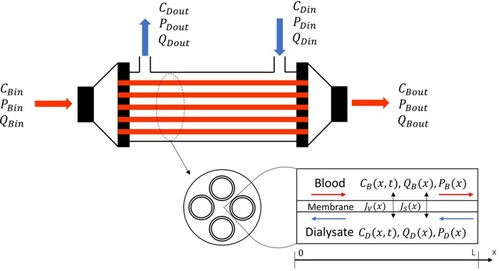
Variables of interest for the problem include the volumetric flow rate Q, pressure P and density ρ. The water filtration and solute fluxes across the membrane are given by J_v and J_s, respectively. The number of fibres (length L, internal diameter d_B and wall thickness δ) inside the dialyser is N. The subscripts B, D and W refer to blood, dialysate and water, respectively, while the subscripts in and out denote inlet and outlet sections, respectively. Figure 1 summarizes some of the variables of interest for the problem.

Figure 1. Dialyser and basic variables.

The mathematical model used here is similar to those presented by Legallais et al [8] and Lee et al [15], but we consider transients in the solute concentrations. Transient concentrations of solutes have been considered by Waniewski et al [21] and Maheshwari et al [22,23]. On the other hand, differently from the model of this work, the momentum balance equation was not solved in [21–23], where the water flux across the membrane was assumed uniform along the dialyser.

The mass balances for the blood and dialysate are given respectively by: (1a) $\begin{array}{rl}\frac{\mathrm{\partial }({\rho }_B{A}_B)}{\mathrm{\partial }t}& =-\frac{\mathrm{\partial }({\rho }_B{Q}_B)}{\mathrm{\partial }x}-N\pi d_B{\rho }_W{J}_V(x)0<x<L,t>0\end{array}$(1a) (1b) $\begin{array}{rl}\frac{\mathrm{\partial }({\rho }_D{A}_D)}{\mathrm{\partial }t}& =\frac{\mathrm{\partial }({\rho }_D{Q}_D)}{\mathrm{\partial }x}+N\pi d_B{\rho }_W{J}_V(x)0<x<L,t>0\end{array}$(1b)

By assuming that blood, dialysate and water densities are constant and equal, Equations (1a,b) reduce respectively to: (2a) $\begin{array}{rl}\frac{\mathrm{\partial }{Q}_B}{\mathrm{\partial }x}& =-N\pi d_B{J}_V(x)0<x<L\end{array}$(2a) (2b) $\begin{array}{rl}\frac{\mathrm{\partial }{Q}_D}{\mathrm{\partial }x}& =-N\pi d_B{J}_V(x)0<x<L\end{array}$(2b) with boundary conditions given by constant inflow rates, that is: (2c) $\begin{array}{rl}{Q}_B(0)& =Q_{Bin}\text{at}x=0\end{array}$(2c) (2d) $\begin{array}{rl}{Q}_D(L)& =Q_{Din}\text{at}x=L\end{array}$(2d)

The water filtration flux across the membrane is given by [8,15]: (3) $J_V(x)=L_P[P_B(x)-P_D(x)-\mathrm{\Pi }(x)]$(3) where L_p is the membrane hydraulic permeability and Π(x) is the local oncotic pressure. This is the osmotic pressure induced by proteins, which tends to bring water back to the blood flowing inside the capillaries. Legallais et al [8] and Lee et al [15] used the following model for the oncotic pressure: (4) $\mathrm{\Pi }(x)=0.21C_p(x)+1.6\times {10}^{-3}[C_p(x){]}^2+9\times {10}^{-6}[C_p(x){]}^3$(4) where C_p(x) is the local plasma protein concentration.

The pressures on the blood and dialysate sides can be computed from the momentum balances. By assuming constant inflow rates and neglecting the momentum transfer across the membrane we obtain [8]: (5a) $\begin{array}{rl}\frac{\mathrm{\partial }{P}_B}{\mathrm{\partial }x}& =-\frac{128{\mu }_B}{N\pi {(d_B)}^4}{Q}_B(x)0<x<L\end{array}$(5a) (5b) $\begin{array}{rl}\frac{\mathrm{\partial }{P}_D}{\mathrm{\partial }x}& =\frac{32{\mu }_D}{A_D{(d_{eq})}^2}{Q}_D(x)0<x<L\end{array}$(5b) where A_D is the area of the cross-section of the dialysate flow: (6) $A_D=\frac{\pi d_{case}^2}{4}-\frac{N\pi {(d_B+2\delta )}^2}{4}$(6) while d_case is the internal diameter of the cylindrical case of the dialyser and d_eq is the hydraulic diameter of dialysate cross-section, that is, (7) $d_{eq}=\frac{4A_D}{N\pi (d_B+2\delta )+\pi d_{case}}$(7)

Boundary conditions for the momentum equations are given by constant outlet pressures, that is: (8a) $\begin{array}{rl}{P}_B(L)& =P_{Bout}\text{at}x=L\end{array}$(8a) (8b) $\begin{array}{rl}{P}_D(0)& =P_{Dout}\text{at}x=0\end{array}$(8b)

The equations for the conservation of a solute are given by: (9a) $\begin{array}{rl}{A}_B\frac{\mathrm{\partial }{C}_B}{\mathrm{\partial }t}& =-\frac{\mathrm{\partial }(Q_B{C}_B)}{\mathrm{\partial }x}-N\pi d_B{J}_s(x)0<x<L,t>0\end{array}$(9a) (9b) $\begin{array}{rl}{A}_D\frac{\mathrm{\partial }{C}_D}{\mathrm{\partial }t}& =\frac{\mathrm{\partial }(Q_D{C}_D)}{\mathrm{\partial }x}+N\pi d_B{J}_s(x)0<x<L,t>0\end{array}$(9b) with boundary conditions (9c) $\begin{array}{rl}{C}_B(0,t)& =C_{Bin}\text{at}x=0,t>0\end{array}$(9c) (9d) $\begin{array}{rl}{C}_D(L,t)& =C_{Din}\text{at}x=L,t>0\end{array}$(9d) and initial conditions (9e) $\begin{array}{rl}{C}_B(x,0)& =C_{Bin},0<x<L,t=0\end{array}$(9e) (9f) $\begin{array}{rl}{C}_D(x,0)& =C_{Din},0<x<L,t=0\end{array}$(9f)

The transmembrane solute flux can be computed from [8]: (10) $J_s(x)=K_o(t)[C_B(x,t)-C_D(x,t)]+J_V(x)S_a[f_B(x)C_B(x,t)+f_D(x)C_D(x,t)]$(10) where K₀(t) is the global mass transfer coefficient for null water filtration flux. We note that this coefficient was considered as time dependent in this work to account for possible fibre clogging or protein layering on the surface of the membrane, during the haemodialysis therapy. The global mass transfer coefficient takes into account the diffusion through the membrane in the form of the coefficient P_m, as well as the mass transfer coefficients on the blood and dialysate sides, K_B and K_D, respectively, and can be written in terms of series resistance as: (11) $\frac{1}{K_0(t)}=\frac{1}{K_B(t)}+\frac{1}{P_m(t)}+\frac{1}{K_D(t)}$(11)

In Equation (10), S_a is the sieving coefficient, while f_B and f_D are respectively the following concentration factors [8,31]: (12a) $\begin{array}{rl}{f}_B& =\frac{\exp [(S_a{J}_V/P_m)+(J_V/K_B)+(J_V/K_D)]}{(1-S_a)\exp (J_V/K_D)[\exp (S_a{J}_V/P_m)-1]+S_a\exp [(S_a{J}_V/P_m)+(J_V/K_B)+(J_V/K_D)]-S_a}\\ & -\frac{K_o}{J_V{S}_a}\end{array}$(12a) (12b) $\begin{array}{rl}{f}_D& =\frac{-1}{(1-S_a)\exp (J_V/K_D)[\exp (S_a{J}_V/P_m)-1]+S_a\exp [(S_a{J}_V/P_m)+(J_V/K_B)+(J_V/K_D)]-S_a}\\ & +\frac{K_o}{J_V{S}_a}\end{array}$(12b)

For the direct problem, all the input parameters and functions in Equations (2) to (12) are known. The direct problem was solved by finite volumes with an upwind explicit scheme [32,33]. With the solution of the direct problem, the solute clearance can be computed as: (13) $C_L=\frac{Q_{Bin}{C}_{Bin}-Q_{Bout}{C}_{Bout}}{C_{Bin}}$(13)

State estimation problem

State estimation problems utilize the information provided by mathematical models and measurements to make inference on the posterior distribution of state variables, which describe the system of interest. Modelling and measurement uncertainties must be appropriately taken into account in the solution of state estimation problems, which aim at the minimization of estimation errors [24–30].

State estimation problems are formulated in terms of two stochastic models, namely: (i) The evolution model and (ii) The observation model. In a discrete approach, these two models correspond, respectively, to the mathematical formulations to advance the posterior distribution of the state variables by one time step, say from time $t_{k-1}$ to time $t_k$, and to relate the state variables to the measurements. Therefore, processes involved in the system under analysis and in the measurements are taken into account by the evolution and observation models, respectively. The fidelity levels of these models depend on the hypotheses assumed for their mathematical formulations, as well as on the accuracies imposed for their computational solutions.

The state evolution model and the observation model are defined here by the functions ${\mathbf{\text{f}}}_k$ and ${\mathbf{\text{g}}}_k$, respectively, and can be written in the following general nonlinear forms [24–30]: (14a) $\begin{array}{rl}{\mathbf{\text{y}}}_k& ={\mathbf{\text{f}}}_k({\mathbf{\text{y}}}_{k-1},\mathit{\theta },{\mathbf{\text{v}}}_k),k=1,\dots ,M\end{array}$(14a) (14b) $\begin{array}{rl}{\mathbf{\text{z}}}_k& ={\mathbf{\text{g}}}_k({\mathbf{\text{y}}}_k,\mathit{\theta },{\mathbf{\text{n}}}_k),k=1,\dots ,M\end{array}$(14b) where the subscript k denotes the time instant $t_k$, ${\mathbf{\text{y}}}_k$ is the vector of state variables, ${\mathbf{\text{z}}}_k$ is the vector resulting from the observation model that corresponds to the measured variables, $\mathit{\theta }$ is a vector containing all the non-dynamic parameters of both models, while ${\mathbf{\text{v}}}_k$ and ${\mathbf{\text{n}}}_k$ represent the noises in the state evolution model and in the observation model, respectively.

For the solution of the state estimation problem, the probability density of the state variables at the initial time t = 0_, $\pi ({\mathbf{\text{y}}}_0,\mathit{\theta }|{\mathbf{\text{z}}}_0)=\pi ({\mathbf{\text{y}}}_0,\mathit{\theta })$, is supposed known. The state estimation problem of this work is solved with the Sampling Importance Resampling (SIR) algorithm of the particle filter method [24–27]. This is a sequential Monte Carlo method, where the posterior probability density function of the state variables is represented by a set of random samples (particles) with associated weights. We denote the particles by ${\mathbf{\text{y}}}_k^i$ and their corresponding weights by $w_k^i,i=1,\dots ,N_p$. In the SIR algorithm, resampling of the particles is performed every time step in order to avoid the degeneracy phenomenon, which is characterized by only few particles with large weights and many particles with negligible weights. Therefore, this is a quite effective algorithm, which involve simple steps that can be readily applied to any state estimation problem, including those with nonlinear and non-Gaussian models. We note that the SIR algorithm may result in sample impoverishment, where many particles exhibit the same value [24–30]. On the other hand, this deleterious effect was not observed in this work as will be apparent below. The basic steps of the SIR algorithm are summarized in Table 1.

Table 1. Sampling Importance Resampling (SIR) Algorithm [27].

Step 1

For $i=1,\dots ,N_p$, draw new particles ${\mathbf{y}}_k^i$ from the prior density $\pi ({\mathbf{y}}_k|{\mathbf{y}}_{k-1}^i,\mathit{\theta })$and then use the likelihood density to calculate the corresponding weights $w_k^i=\pi ({\text{z}}_k|{\mathbf{y}}_k^i,\mathit{\theta })$.

Step 2

Calculate the total weight $T_w=\sum _{i=1}^{N_p}{w}_k^i$ and then normalize the particle weights, that is, for $i=1,\dots ,N_p$ let $w_k^i=T_w^{-1}{w}_k^i$.

Step 3

Resample the particles as follows:

Construct the cumulative sum of weights (CSW) by computing

$c_i=c_{i-1}+w_k^i$ for $i=1,\dots ,N_p$, with $c_0=0$.

Let $i=1$ and draw a starting point $u_1$ from the uniform distribution $U[0,N_p^{-1}]$.

For $j=1,\dots ,N_p$

Move along the CSW by making $u_j=u_1+N_p^{-1}(j-1)$

While $u_j>c_i$ make $i=i+1$ and

Assign sample ${\mathbf{y}}_k^j={\mathbf{y}}_k^i$

Assign sample weight $w_k^j=N_p^{-1}$.

The SIR algorithm of the particle filter method was applied below for the estimation of the transient solute concentrations in the blood and dialysate, as well as of the transient global mass transfer coefficient, K₀(t). Therefore, the vector of state variables is given by: (15) $\mathbf{\text{y}}(t)=\left[\begin{array}{c}{\mathbf{\text{C}}}_B(t)\\ {\mathbf{\text{C}}}_D(t)\\ K_0(t)\end{array}\right]$(15) where the vectors C_B(t) and C_D(t) contain the solute concentrations in the blood and the dialysate, respectively, in all finite volumes used for the discretization of the dialyser.

The evolution models for C_B(t) and C_D(t) are given by the discrete form of the direct problem presented in the previous section. Uncertainties for these state variables were supposed additive, uncorrelated, Gaussian, with zero means and constant covariance matrix.

No information was a priori assumed for the functional form of the global mass transfer coefficient, K₀(t). Therefore, the evolution model for this state variable was given by an independent Markovian process with a Gaussian distribution of zero mean and standard deviation ${\sigma }_{K_0}^{}(t_{k-1})$, that is, (16) $K_0^{}(t_k)=K_0^{}(t_{k-1})+{\sigma }_{K_0}^{}(t_{k-1}){\phi }_{k-1}$(16) where ${\phi }_{k-1}$ is a random Gaussian number with zero mean and unitary standard deviation.

Measurements of the dialysate outlet solute concentration were assumed sequentially available for the solution of the state estimation problem. The measurements were supposed uncorrelated and containing additive Gaussian noises, with zero means and constant standard deviation ${\sigma }_{meas}^{}$. Therefore, the observation model for the measurement at time $t_k$ can be written as: (17) $z_k=g_k({\mathbf{\text{y}}}_k^{},\mathit{\theta })+n_k$(17) where the function $g_k({\mathbf{\text{y}}}_k^{},\mathit{\theta })$ selects $C_{Dout}(t_k)$ from the state vector ${\mathbf{\text{y}}}_k^{}$.

With the above hypotheses about the measurement errors, the likelihood function, which is used for the computation of the weights in the particle filter method, is thus given by: (18) $\pi (z_k|{\mathbf{\text{y}}}_k\mathbf{,}\mathit{\theta })=\frac{1}{{\sigma }_{\text{meas}}\sqrt{2\text{π}}}\exp \left\{-\frac{1}{2}\frac{{[z_k^{\text{meas}}-g_k({\mathbf{\text{y}}}_k,\mathit{\theta })]}^2}{{\sigma }_{\text{meas}}^2}\right\}$(18) where $\text{π}=3.1415$ and $z_k^{\text{meas}}$ is the measurement at time $t_k$.

The vector of model parameters, θ, was supposed known in this work, but their related uncertainties were accounted for in the vector ${\mathbf{\text{v}}}_k^{}$ by performing a Monte Carlo direct simulation, as explained below.

Results and discussions

The results presented below involve only one solute, creatinine, and constant flow rates Q_B = 200 ml/min and Q_D = 500 ml/min. The inlet concentrations of creatinine for the blood and dialysate were supposed as C_Bin = 0.124 mg/ml and C_Din = 0 mg/ml, respectively. The dialyser parameters used in the simulations are presented in Table 2, which correspond to the model Hospal Filtral 12 [8]. For creatinine, the sieving coefficient S_a was taken equal to 1, while the global mass transfer coefficient reference value was assumed as 4.26 × 10⁻⁶ m/s [7,8]. The mass transfer resistances on the blood and dialysate sides were assumed negligible, based on the hypotheses that fluid solute concentrations are uniform and that there is no discontinuity of the solute concentrations in the fluids and at the membrane surfaces. Therefore, from Equation (11), K₀(t) = P_m(t). For the calculation of the oncotic pressure given by Equation (4), the protein concentration in the blood was assumed constant (C_p(x) = 10 mg/ml), since proteins are not transferred through the membrane.

Table 2. Parameters of the dialyser Hospal Filtral 12 [8].

Effective length	L = 0.20 m
Number of fibres	N = 8500
Inner diameter of fibres	dB = 220 µm
Fibre thickness	δ= 45 µm
Case diameter	dcase = 0.039 m
Membrane hydraulic permeability	Lp = 27 ml/(h m^2 mmHg)

This work´s numerical solution of the direct problem was verified with an analytical solution for the steady-state, in a case involving only diffusion across the membrane. The agreement between the numerical and the analytical solutions is perfect at the graph scale, as shown by Figure 2. Furthermore, the solution was also verified by using the results presented in [8] for the clearance of creatinine, with imposed filtration flow rates of Q_f = 20, 40 and 60 ml/min. The results presented by Legallais et al [8] and those of this work are in excellent agreement, as shown by Table 3. This table shows the values of the increase in creatinine clearance, $C_L$, relative to the clearance obtained with diffusion only (Q_f = 0), $C_{L_0}$.

Figure 2. Comparison of numerical and analytical solutions of the direct problem with diffusion only across the membrane.

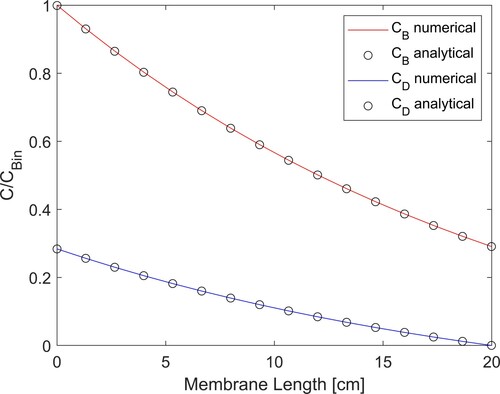
Table 3. Comparison with the clearances obtained by Legallais et al [8].

	Relative Increase of Creatinine Clearance, $(C_L-C_{L_0})/C_{L_0}$
Qf, ml/min	Legallais et al [8]	This work
20	0.053	0.058
40	0.107	0.108
60	0.160	0.158

For all cases examined below, the standard deviation for the random walk evolution model for K₀(t) (see equation 1(1a) $\begin{array}{rl}\frac{\mathrm{\partial }({\rho }_B{A}_B)}{\mathrm{\partial }t}& =-\frac{\mathrm{\partial }({\rho }_B{Q}_B)}{\mathrm{\partial }x}-N\pi d_B{\rho }_W{J}_V(x)0<x<L,t>0\end{array}$(1a) 6) was set as ${\sigma }_{K_0}^{}(t_k)=0.02K_0^{}(t_k)$. This standard deviation was selected by numerical experiments and avoided a large lag in step variations in K₀(t), as well as instabilities inherent of the ill-posed character of the inverse problem. The simulated measurements were generated from the solution of the direct problem with different functional forms for K₀(t). Gaussian errors with zero mean and constant standard deviation 0.01C_Bin were added to the solution of the direct problem. The measurements were considered available with a frequency of either 1 Hz or 10 Hz, during 100 s. Hence, this study was focused at the very first stage of the HD therapy.

The standard deviations for the uncorrelated Gaussian uncertainties in the evolution models of C_B and C_D were assumed constant and respectively equal to 1.5% and 1% of the inlet blood concentration, C_Bin. These uncertainties in the evolution model resulted from a direct Monte Carlo simulation performed with Gaussian priors for the model parameters, centred on the values presented above and with standard deviations of 2% of the means. As for the distributions of the state variables at time t = 0, their means were given by the initial conditions assigned to the evolution model and the corresponding standard deviations were the same presented above.

We first analyse cases where the water filtration rate through the membrane is zero (Q_f = 0 ml/min), that is, the solute transfer from the blood to dialysate takes place by diffusion only. Table 4 presents the RMS errors given by Equation (19) for the estimated mass transfer coefficient, by considering different numbers of particles in the SIR algorithm. In Equation (19), ${\overline{K}}_0(t_k)$ is the mean estimated with the particle filter and $K_{0\text{,exa}}(t_k)$ is the exact value used to generate the simulated measurements. Computational times for the inverse problem solution are also presented in Table 4. Computations were performed with an in-house code run in Matlab, by using a computer with an [email protected] GHz processor and 16 Gbyte of RAM memory. The simulated measurements used for the results presented in Table 4 were generated with a frequency of 10 Hz, by considering that the membrane mass transfer coefficient suddenly decreased from its reference value 4.26 × 10⁻⁶ m/s to 2.13 × 10⁻⁶ m/s, as a step variation at time t = 50 s. Table 4 shows that the RMS error reduced by 24% when the number of particles increased from 2000 to 2500 and then by 15% when it increased from 3000 to 5000. On the other hand, these reductions in the RMS errors involved computational time increases by factors of 3.7 and 5.3, respectively, due to the larger number of particles that also resulted in larger matrix terms required for the calculations. Even with an interpreted language as Matlab, the application of the particle filter can be performed in real-time with 2000 particles, since the computational time is smaller than the simulated time of 100 s. The computational time was 2.36 times higher than the simulated time when 2500 particles were used in the SIR algorithm. 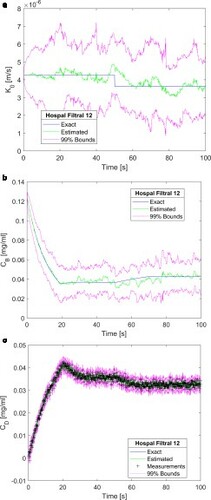(19) $e_{RMS}=\sqrt{\frac{1}{M}\sum _{k=1}^M[{\overline{K}}_0(t_k)-K_{0\text{,exa}}(t_k)]}$(19) Figure 3a-c present the estimated mass transfer coefficient, the estimated blood concentration of creatinine returning to the patient, as well as the estimated and simulated measured concentrations of creatinine in the dialysate at the outlet of the dialyser, respectively, obtained with 2000 particles. The mass transfer coefficient step function used to generate the simulated measurements (see Figure 3a) was the same for which the RMS errors are presented in Table 4. The estimated mean mass transfer coefficient is in good agreement with the exact function used to generate the simulated measurements, as shown by Figure 3a, despite the fact that no prior information was assumed available and the evolution model for this state variable was given by the random walk process of Equation (16). Uncertainties in the estimated mass transfer coefficient were in general large, but encompassed the exact functional form. Both the mean values and the 99% confidence intervals follow the discontinuity in $K_0(t)$. 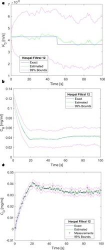The creatinine concentration in the blood returning to the patient was estimated with small uncertainties and with means in excellent agreement with the exact solution, as shown by Figure 3b. Figure 3c shows that the estimated dialysate concentration is in excellent agreement with the measurements and their related uncertainties are of the same order of magnitude. Oscillations observed in the estimated mass transfer coefficient and in the creatinine concentration of the blood returning to the patient can be reduced by increasing the number of particles to 2500, as shown by Figure 4a-c. As expected from the analysis of table 4, a comparison of Figures 3 and 4 reveals that the agreement between estimated and exact state variables improved when the number of particles increased from 2000 to 2500. In particular, the estimated mass transfer coefficient and the associated 99% confidence intervals were smoother and better reflected the step reduction at time t = 50 s. Therefore, the results presented heretofore were obtained with 2500 particles in the SIR algorithm.

Figure 3. Results obtained for a step reduction of 50% in the membrane mass transfer coefficient – Measurement frequency of 10 Hz and 2000 particles: (a) Mass transfer coefficient; (b) Creatinine concentration returning to the patient; (c) Creatinine concentration in the dialysate at the dialyser outlet.

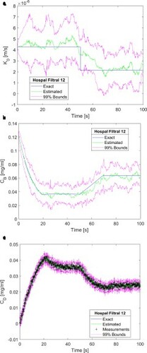
Figure 4. Results obtained for a step reduction of 50% in the membrane mass transfer coefficient – Measurement frequency of 10 Hz and 2500 particles: (a) Mass transfer coefficient; (b) Creatinine concentration returning to the patient; (c) Creatinine concentration in the dialysate at the dialyser outlet.

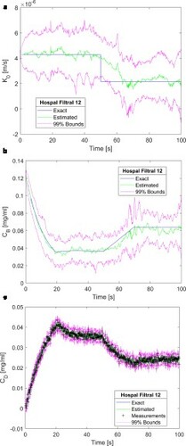
Table 4. RMS errors and CPU times for a step variation of the mass transfer coefficient.

Number of Particles	RMS Error, m/s	Computational Time, s
1000	6.9 × 10^−7	29.7
1500	6.9 × 10^−7	44.9
2000	7.0 × 10^−7	63.5
2500	5.3 × 10^−7	236.5
3000	5.4 × 10^−7	1296
5000	4.6 × 10^−7	6891

Results similar to those presented in Figure 4a-c are shown by Figure 5a-c, but with the step reduction in the mass transfer coefficient of 15% of the reference value, that is, $K_0(t)$varied from 4.26 × 10⁻⁶ m/s to 3.62 × 10⁻⁶ m/s. This test case was examined in order to assess the accuracy of the SIR algorithm under very strict situations for the inverse problem solution that might be observed in practice, involving small reductions in the membrane mass transfer coefficient when the HD therapy begins. The results presented in Figure 5a-c were also obtained with a measurement frequency of 10 Hz. A comparison of Figures 4 and 5 reveals that the agreement between the estimated means and the exact state variables was not affected by the magnitude of the mass transfer coefficient reduction. In fact, we note in Figure 5a that even a small variation of only 15% in the mass transfer coefficient, and its effects on the blood and dialysate outlet concentrations (see Figure 5b and c, respectively), could be recovered by the solution of the state estimation problem with the SIR algorithm. Although the estimated means and the 99% confidence intervals followed the step variation in $K_0(t)$ (Figure 5a), uncertainties in this state variable were large and would not allow any distinction between the two levels of the step function in this case. On the other hand, the creatinine concentrations at the blood outlet (Figure 5b) and at the dialysate outlet (Figure 5c) were estimated with small uncertainties.

Figure 5. Results obtained for a step reduction of 15% in the membrane mass transfer coefficient – Measurement frequency of 10 Hz and 2500 particles: (a) Mass transfer coefficient; (b) Creatinine concentration returning to the patient; (c) Creatinine concentration in the dialysate at the dialyser outlet.

We now examine the effects of the measurement frequency on the solution of the state estimation problem. The results obtained with a step reduction of 15% in $K_0(t)$ and a measurement frequency of 1Hz are presented by Figure 6a-c for the mass transfer coefficient, creatinine concentration at the blood outlet and creatine concentration at the dialysate outlet, respectively. As compared to the results obtained with a measurement frequency of 10 Hz (see Figure 5a-c), Figure 6a-c show that the estimated means and confidence intervals became smoother when the measurement frequency was reduced. This behaviour is due to the ill-posed character of the problem, which became less regularized as the measurements were assimilated with a larger frequency.

Figure 6. Results obtained for a step reduction of 15% in the membrane mass transfer coefficient – Measurement frequency of 1 Hz and 2500 particles: (a) Mass transfer coefficient; (b) Creatinine concentration returning to the patient; (c) Creatinine concentration in the dialysate at the dialyser outlet.

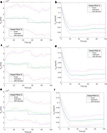
Figure 6a-c demonstrate that the measurement frequency of 1Hz was appropriate to obtain accurate and stable solutions for this problem. Therefore, this frequency was considered for the results presented in Figure 7, which involved filtration flow rates of Q_f = 20, 40 and 60 ml/min. With the imposed outlet boundary pressures (see Equations 7), the inlet pressures were iteratively adjusted to provide these values of filtration rates. Figure 7 presents the results obtained with Q_f = 20, 40 and 60 ml/min, for the mass transfer coefficient (Figure 7a, c and e) and for the creatinine in the blood returning to the patient (Figure 7b, d and f), respectively. A comparison of Figures 6 and 7 demonstrates that the quality of the estimation of the state variables was not affected by the filtration rate across the membrane.

Figure 7. Results obtained for a step reduction of 15% in the membrane mass transfer coefficient – Measurement frequency of 1 Hz and 2500 particles: (a) Mass transfer coefficient (Q_f = 20 ml/min); (b) Creatinine concentration returning to the patient (Q_f = 20 ml/min); (c) Mass transfer coefficient (Q_f = 40 ml/min); (d) Creatinine concentration returning to the patient (Q_f = 40 ml/min); (e) Mass transfer coefficient (Q_f = 60 ml/min); (f) Creatinine concentration returning to the patient (Q_f = 60 ml/min).

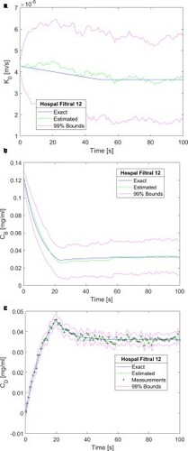
Finally, a functional form different from the step variation was examined for $K_0(t)$. We considered a linear reduction of 15% in the mass transfer coefficient from 4.26 × 10⁻⁶ m/s at t = 0 s to 3.62 × 10⁻⁶ m/s at t = 50 s, followed by this constant value. The results obtained with a frequency of 1 Hz and Q_f = 60 ml/min are presented by Figure 8a-c. For this functional form, the SIR algorithm was also capable of accurately estimating the mass transfer coefficient function (see Figure 8a), thus resulting in accurate estimations of the creatinine blood concentrations at the blood and dialysate sides of the dialyser, as shown by Figures 8b and c, respectively.

Figure 8. Results obtained for a linear reduction of 15% followed by a constant value of the membrane mass transfer coefficient – Measurement frequency of 1 Hz, 2500 particles and Q_f = 60 ml/min: (a) Mass transfer coefficient; (b) Creatinine concentration returning to the patient; (c) Creatinine concentration in the dialysate at the dialyser outlet.

Results similar to those presented above were also obtained with dialysers of larger area, as well as for urea. These results are not presented here for the sake of brevity.

Conclusions

This work was aimed at the transient analysis of a haemodialyser, which undergoes a reduction in the solute mass transfer coefficient of the capillary membrane. Such a reduction can be caused, for example, by fibre clogging or protein layering. A state estimation problem was solved with the Sampling Importance Resampling (SIR) algorithm of the particle filter method, which provided accurate estimations of the transient mass transfer coefficient and, in particular, of the creatinine concentration in the blood returning to the patient after passing through the haemodialyser. No prior assumption was assumed available regarding the functional form of the mass transfer coefficient, which was modelled as an independent Markovian process. The SIR algorithm was applied with 2500 particles, which resulted in small RMS errors for the estimation of the mass transfer coefficient and did not present sample impoverishment for the cases examined.

The model used in this work did not include the water and solute dynamics within the patient´s body, nor transient boundary conditions for the flow rates, pressures and solute concentrations. These simplifications can be justified by the short time period considered for the cases examined, which was of 100 s during the very first stage of the HD therapy. The dialyser certainly needs to be coupled to the patient´s body dynamics in a model more appropriate for an actual haemodialysis session, which can last few hours. Moreover, other solutes need to be included in the analysis, besides creatinine. Despite these simplifications, the SIR algorithm resulted in estimated means that were stable and in excellent agreement with the exact state variables. The quality of the estimations was not affected by the imposed water filtration rate, measurement frequency and functional form of the simulated reduction in the membrane mass transfer coefficient. The computational times associated with the particle filter solutions might allow the use of this technique in real-time applications, such as online monitoring and/or control.

Acknowledgement

The support provided by CNPq and FAPERJ, agencies of the Brazilian and Rio de Janeiro state governments, is gratefully appreciated. This study was financed in part by Coordenação de Aperfeiçoamento de Pessoal de Nível Superior - Brazil (CAPES) - Finance Code 001.

Disclosure statement

No potential conflict of interest was reported by the author(s).

Additional information

Funding

This work was supported by Conselho Nacional de Desenvolvimento Científico e Tecnológico: [grant PQ]; Coordenação de Aperfeiçoamento de Pessoal de Nível Superior: [grant number Fincance Code 001]; Fundação Carlos Chagas Filho de Amparo à Pesquisa do Estado do Rio de Janeiro: (Cientista do Estado).

References

- Levey A, Coresh J. Chronic kidney disease. Lancet. 2012;379:165–180.
- Ronco C, Canaud B, Aljama P., editors. Hemodiafiltration (Vol. 158). Basel: Karger Medical and Scientific Publishers; 2007.
- Drukker W, Parsons FM, Maher JF., editors. Replacement of renal function by dialysis: a textbook of dialysis. Dordrecht: Springer Science & Business Media; 2012.
- Twardowski ZJ. History of hemodialyzers’ designs. Hemodial Int. 2008;12(2):173–210.
- Locatelli F, Buoncristiani U, Canaud B, et al. Haemodialysis with on-line monitoring equipment: tools or toys? Nephrol Dial Transplant. 2005;20:22–33.
- Abbrecht PH, Prodany NW. A model of the patient-artificial kidney system. Trans On Bio Engin. 1971;18:257–264.
- Jaffrin MY, Ding L, Laurent JM. Simultneous convective and diffusive mass transfers in hemodialyzer. J Bio Eng. 1990;112: 112–212.
- Legallais C, Catapano G, Harten B, et al. A theoretical model to predict the in vitro performance of hemodiafilters. J Membr Sci. 2000;168:3–15.
- Lambie SH, McIntyre CW. Developments in online monitoring of haemodialysis patients: towards global assessment of dialysis adequacy. Curr Opin Nephrol Hypertens. 2003;12(6):633–638.
- Uhlin F, Fridolin I, Magnusson M, et al. Dialysis dose (Kt/V) and clearance variation sensitivity using measurement of ultraviolet-absorbance (on-line), blood urea, dialysate urea and ionic dialysance. Nephrol Dial Transplant. 2006;21(8):2225–2231.
- Nigatie Y. Diffusion in tube dialyzer. Biomed Eng Comput Biol. 2017;8:1179597217732006.
- Islam MS, Szpunar J. Study of dialyzer membrane (Polyflux 210H) and effects of different parameters on dialysis performance. Open J Nephrol. 2013;3:161–167.
- Tam VK. The mathematical basis, clinical application and limitations of ionic dialysance. Hong Kong J Nephrol. 2004;6(1):56–59.
- Droog RP, Kingma BR, van Marken Lichtenbelt WD, et al. Mathematical modeling of thermal and circulatory effects during hemodialysis. Artif Organs. 2012;36(9):797–811.
- Lee JC, Lee K, Kim HC. Mathematical analysis for internal filtration of convection-enhanced high-flux hemodialyzer. Comput Methods Programs Biomed. 2012;108(1):68–79.
- Leypoldt JK, Storr M, Agar BU, et al. Intradialytic kinetics of middle molecules during hemodialysis and hemodiafiltration. Nephrol Dial Transplant. 2019;34(5):870–877.
- Schneditz D, 2001. Temperature and thermal balance in hemodialysis. In Seminars in dialysis (Vol. 14, No. 5). New York (US): Blackwell Science Inc., p. 357–364. DOI:https://doi.org/10.1046/j.1525-139X.2001.00088.x.
- Bianchi C, Lanzarone E, Casagrande G, et al. 2016. Identification of patient-specific parameters in a kinetic model of fluid and mass transfer during dialysis. In: Argiento R, Lanzarone E, Villalobos IA, Mattei A, editors. International conference on Bayesian statistics in action. Cham: Springer, 2016. p. 139–149.
- Bianchi C, Lanzarone E, Casagrande G, et al. A Bayesian approach for the identification of patient-specific parameters in a dialysis kinetic model. Stat Methods Med Res. 2019;28(7):2069–2095.
- Casagrande G, Bianchi C, Vito D, et al. Patient-specific modeling of multicompartmental fluid and mass exchange during dialysis. Int J Artif Organs. 2016;39:220–227.
- Waniewski J, Poleszczuk J, Pietribiasi M, et al. Impact of solute exchange between erythrocytes and plasma on hemodialyzer clearance. Biocybern Biomed Eng. 2020;40:265–276.
- Maheshwari V, Thijssen S, Tao X, et al. In silico comparison of protein-bound uremic toxin removal by hemodialysis, hemodiafiltration, membrane adsorption, and binding competition. Nat Sci Rep. 2019;9(1):1–13.
- Maheshwari V, Thijssen S, Tao X, et al. A novel mathematical model of protein-bound uremic toxin kinetics during hemodialysis. Nat Sci Rep. 2017;7(1):1–15.
- Doucet A, De Freitas N, Gordon N. Sequential Monte Carlo methods in practice. New York: Springer; 2001; 178–195.
- Kaipio J, Somersalo E. (2004). Statistical and computational inverse problems, Applied Mathematical Sciences 160, Springer-Verlag.
- Ristic B, Arulampalam S, Gordon N. Beyond the Kalman filter. Boston: Artech House; 2004.
- Arulampalam MS, Maskell S, Gordon N, et al. A tutorial on particle filters for online nonlinear/non-Gaussian Bayesian tracking. IEEE Trans Signal Process. 2002;50:174–188.
- Orlande HRB, Colaço MJ, Dulikravich GS, et al. State estimation problems in heat transfer. Int J Uncertainty Quant. 2012;2:239–258.
- Lamien B, Varon L, Orlande H. State estimation in bioheat transfer: a comparison of particle filter algorithms. Int J Numer Methods Heat Fluid Flow. 2017;27:615–638.
- Costa J, Orlande H, Campos Velho H, et al. Estimation of tumor size evolution using particle filters. J Comput Biol. 2015;22:150514113004000.
- Zydney AL. Bulk mass transport limitations during high-flux hemodialysis. Artif Organs. 1993;17(11):919–924.
- Patankar SV. Numerical heat transfer and fluid flow. New York: Taylor & Francis; 1980.
- Ozisik M, Orlande H, Colaco M, et al. Finite difference methods in heat transfer. 2nd ed. Boca Raton: CRC Press; 2017.