Identification of the air gap thermal resistance in the model of binary alloy solidification including the macrosegregation and the material shrinkage phenomena

Abstract

Goal of this elaboration is to investigate the mathematical model of the inverse problem of binary alloy solidification within the casting mould, with the material shrinkage and the macrosegregation phenomena included simultaneously. Major result of this paper is the solution of the inverse problem consisting in reconstruction of the following elements: the thermal resistance of the air gap created between the cast and the mould in the course of solidification process and the heat transfer coefficient on the boundary of heat exchange between the mould and environment. The additional information, necessary to solve the inverse task, is delivered by the temperature measurements read in the control point located in the centre of the mould. The theoretical discussion is supported by the numerical examples executed for various sets of input data.

Keywords:

• Solidification
• binary alloy
• macrosegregation
• material shrinkage
• swarm intelligence

2010 Mathematics Subject Classifications:

• 80A23
• 80M20
• 80M50
• 97R40

Nomenclature

$b,d_0$	=	Dimensions of the mould
c	=	Specific heat
C	=	Substitute thermal capacity
$d(t)$	=	Thickness of the plate
$f_s$	=	Volumetric solid state fraction
h	=	Heat transfer coefficient
J	=	Minimized functional
k	=	Thermal conductivity
L	=	Latent heat of solidification
m	=	Mass
$m_0$	=	Mass of the alloy
N	=	Number of measurements
R	=	Thermal resistance
t	=	Time
T	=	Temperature
$T_L$	=	Liquidus temperature
$T_S$	=	Solidus temperature
$T_0$	=	Initial temperature
$T_{\mathrm{\infty }}$	=	Ambient temperature
$U_i$	=	Measured temperature
$v_x$	=	Velocity vector
$V_j$	=	Control volume
x	=	Spatial variable
$Z_0$	=	Initial concentration of alloy component
$Z_L$	=	Concentration of alloy component [6pt]

Greek symbols

$\mathrm{\Delta }P$	=	Area of the plate
χ	=	Partition coefficient
ρ	=	Mass density
${\xi }_l,$ ${\xi }_s,$	=	Locations of liquidus and solidus temperatures
Ω	=	Considered region

Subscripts

g	=	Air gap
l	=	Liquid phase
m	=	Mould
mz	=	Mushy zone
s	=	Solid phase

1. Introduction

In present, most of the mathematical models, used in applications, is so much complicated that it is not possible to determine their analytical solution. Therefore, the numerical methods, enabling to compute the approximate solutions of considered equations, became very important. In particular, Dehghan and Abbaszadeh in [1] propose the proper orthogonal decomposition variational multiscale element free Galerkin method for solving the time-dependent incompressible Navier-Stokes equation. Next, in paper [2], the proper orthogonal decomposition approach, compiled with the upwind local radial basis functions–differential quadrature method, is applied for solving the compressible Euler equation. The same authors in work [3] present the meshless weak form to simulate the Oldroyd equation. The authors show that the proposed scheme has a unique solution and examine the error estimation of this method. In paper [4], the numerical simulation and sensitivity analysis are carried out on turbulent heat transfer and heat exchanger effectiveness enhancement in a double pipe heat exchanger filled with porous media. In work [5], the entropy generation analysis is done for nanofluid flow in a channel with wavy walls. The authors investigate an influence of various parameters (Reynolds number, nanoparticle volume fraction, dimensionless amplitude and wave number) on the entropy generation. Next, in paper [6], the response surface methodology and two phase mixture model are proposed to investigate the sensitivity analysis of heat transfer and heat exchanger effectiveness in a double pipe heat exchanger filled with nanofluid.

While solving the physical, technical or engineering tasks many identification, controlling or projecting problems are presented as the inverse problems described by the incompletely defined set of data. From the practical perspective, the inverse problems give possibilities to control various processes, therefore, we find them to be more interesting and more challenging than the direct problems. In particular, in paper [7], the one-dimensional inverse heat conduction problem is investigated. The considered inverse problem consists in reconstruction of the heat flux in the left end of the region, when in the right end two conditions are given. For solving this problem, the authors use the Ritz-Galerkin method with two types of basis functions (Bernstain multi-scaling functions and cubic B-spline functions). The Ritz-Galerkin method is also applied in work [8] for determining the heat source in the one-dimensional heat conduction equation. In paper [9], the author reconstructs the heat flux in the model of binary alloy solidification. The additional information in the inverse problem, considered in this paper, is given by the temperature measurements in the selected point of the alloy. The proposed model includes the change of the alloy component concentration caused by the solidification process of alloy. The solution method is based on the finite difference method and the ant colony optimization algorithm. Reddy and Dulikravich in work [10] consider the two-dimensional inverse problem consisted in simultaneous reconstruction of the thermal conductivity and the specific heat. In this case, the additional information is also delivered by the temperature measurements made in the boundary of the region. The direct problem is solved by using the finite difference method, whereas the proper functional is minimized with the aid of a hybrid method being a combination of the particle swarm optimization and the Broyden–Fletcher–Goldfarb–Shanno optimization algorithm.

In the current paper, we focus on the inverse problem associated to the solidification process of binary alloy within the casting mould and the reconstruction of the air gap thermal resistance.

The purpose of this elaboration is to investigate the mathematical model of the inverse one-dimensional problem of the binary alloy solidifying within the casting mould, with the material shrinkage and the macrosegregation phenomena included. Both phenomena influence the process of solidification – the macrosegregation refers to the variations in composition of the cast, whereas the material shrinkage results in creation of the air gap between the mould and the cast. The phenomena were already discussed in literature separately, they are rather not considered together, like we do in the current paper being the continuation of research initiated in [11]. For example, the authors in [12,13] determine the heat resistance of the gap created between the ingot and the mould or the crystallizer, whereas in [14,15], the models describing the macrosegregation are investigated. The solidification process is described by applying the model of solidification in the temperature interval. In this case, we use the equation of heat conduction enclosing the source element that includes the latent heat of fusion together with the volumetric contribution of the solid state. Such prepared equation describes the temperature distribution in the entire cast composed of three phases: the liquid phase, the mushy zone (in which liquid and solid coexist) and the solid phase [16,17]. In the region of mould, the temperature is distributed according to the ordinary one-dimensional heat conduction equation. Both heat equations are completed by the appropriate initial and boundary conditions. The shrinkage of material is described on the basis of the mass balance equation [12], whereas for modeling the macrosegregation process we apply the Scheil model [18–21].

The goal of the investigated inverse problem is to reconstruct the following elements: the thermal resistance of the air gap formed between the cast and the mould in the course of solidification process and the heat transfer coefficient in the boundary condition defined in the boundary of heat exchange between the mould and environment. The additional information, required for solving the inverse problem, is delivered by the temperature measurements read in the control point localized in the middle of the mould. For the solution of the inverse problem we use two procedures: the implicit scheme of the finite difference method completed by the procedure of correcting the field of temperature in the neighbourhood of liquidus and solidus curves, used for determining the solution of the direct problem connected with the inverse one, and the selected swarm intelligence minimization algorithm, applied for finding the minimum of the functional expressing the differences between the retrieved values of temperature and the values read in the control point. The theoretical discussion is supported by the numerical examples executed for various levels of input data perturbations, various time intervals between the readings of temperature and various settings of the pseudo-random number generator used in the optimization algorithm.

The current paper is the continuation of research initiated in [11], where only one element was reconstructed. The novelty of the proposed approach lies in solving the inverse problem of binary alloy solidification within the casting mould with two phenomena influencing the solidification process, the material shrinkage and the macrosegregation, considered simultaneously in one model. We have not found such model in any literature position, we know. In the solving procedure we use the swarm intelligence algorithm and, what is worth to mention, the numerical experiment for investigating stability and exactness of the method was conducted with the aid of computer programs created entirely by the authors (without using any programming libraries), thanks to which the solution programs can be adapted in every step to any new conditions.

2. Mathematical description of the task

The region of investigated problem is presented in Figure 1. It is the solidifying plate of thickness $d(t)$, described by set $\mathrm{\Omega }=\{(x,t):x\in (0,d(t)),t\in (0,t^{\ast })\}$, whereas the region of casting mould is described by set ${\mathrm{\Omega }}_m=\{(x,t):x\in (d_0,b),t\in (0,t^{\ast })\}$.

Figure 1. Region of the problem.

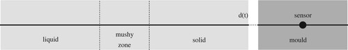
The solidifying material takes three states: liquid, solid and an intermediate state combining the liquid and solid qualities, therefore, the cast region consists of three subregions: occupied by the liquid phase, mushy zone and solid phase. At the beginning of the process, we have the perfect contact between the cast and the mould, that is $d(0)=d_0$, but during the solidification process the solidifying material shrinks by forming the air gap. Thus, the boundary $d(t)$ of the cast is mobile.

The investigated process of solidification is modelled with the aid of well-known (classical) heat conduction equation, completed by the initial and boundary conditions. More information about these equations and their derivation can be found, for example, in books [19,20]. Thus, the temperature field in region Ω is specified by the following heat conduction equation (1) $c\rho \frac{\mathrm{\partial }T(x,t)}{\mathrm{\partial }t}+v_x\frac{\mathrm{\partial }T(x,t)}{\mathrm{\partial }x}=k\frac{{\mathrm{\partial }}^{2}T(x,t)}{\mathrm{\partial }{x}^2}+L\rho \frac{\mathrm{\partial }{f}_s(x,t)}{\mathrm{\partial }t},$(1) where $\rho >0$, c>0 and k>0 denote, respectively, the mass density, specific heat and thermal conductivity coefficient, $v_x>0$ describes the velocity of solidus curve, L>0 means the latent heat of solidification, $f_s$ denotes the volumetric solid state fraction, T refers to the temperature, whereas t and x are the time and spatial variables. The volumetric solid state fraction is dependent on temperature, therefore, by assuming (2) $\frac{\mathrm{\partial }{f}_s}{\mathrm{\partial }t}=\frac{\mathrm{\partial }{f}_s}{\mathrm{\partial }T}\frac{\mathrm{\partial }T}{\mathrm{\partial }t}.$(2) Equation (1(1) $c\rho \frac{\mathrm{\partial }T(x,t)}{\mathrm{\partial }t}+v_x\frac{\mathrm{\partial }T(x,t)}{\mathrm{\partial }x}=k\frac{{\mathrm{\partial }}^{2}T(x,t)}{\mathrm{\partial }{x}^2}+L\rho \frac{\mathrm{\partial }{f}_s(x,t)}{\mathrm{\partial }t},$(1) ), after simple transformation, takes the form (3) $C\rho \frac{\mathrm{\partial }T(x,t)}{\mathrm{\partial }t}+v_x\frac{\mathrm{\partial }T(x,t)}{\mathrm{\partial }x}=k\frac{{\mathrm{\partial }}^{2}T(x,t)}{\mathrm{\partial }{x}^2},$(3) where $C=c-L\frac{\mathrm{\partial }{f}_s}{\mathrm{\partial }t}$ defines the substitute thermal capacity. The equation in form (3(3) $C\rho \frac{\mathrm{\partial }T(x,t)}{\mathrm{\partial }t}+v_x\frac{\mathrm{\partial }T(x,t)}{\mathrm{\partial }x}=k\frac{{\mathrm{\partial }}^{2}T(x,t)}{\mathrm{\partial }{x}^2},$(3) ) defines the heat conduction in the whole investigated domain consisting of three subregions, that is in the liquid zone, in the mushy zone, as well as in the solid zone.

Function $f_s$ must fulfil the conditions: $f_s(T_L(Z_L))=0$ and $f_s(T_S(Z_L))=1,$ where $T_L$ and $T_S$ mean the liquidus and solidus temperatures, so after taking the assumption about the linear dependence of $f_s$ on temperature, which may be found in literature (see [14,15,18]), we assume (4) $\begin{array}{r}{f}_s(T)=\{\begin{array}{ll}{\displaystyle 0}& T>T_L(Z_L),\\ {\displaystyle \frac{T_L(Z_L)-T}{T_L(Z_L)-T_S(Z_L)}}& T\in [T_S(Z_L),T_L(Z_L)],\\ {\displaystyle 1}& T<T_S(Z_L),\end{array}\end{array}$(4) for $T\in [T_S(Z_L),T_L(Z_L)],$ where $Z_L$ denotes the alloy component concentration. Substituting the derivative of function (4(4) $\begin{array}{r}{f}_s(T)=\{\begin{array}{ll}{\displaystyle 0}& T>T_L(Z_L),\\ {\displaystyle \frac{T_L(Z_L)-T}{T_L(Z_L)-T_S(Z_L)}}& T\in [T_S(Z_L),T_L(Z_L)],\\ {\displaystyle 1}& T<T_S(Z_L),\end{array}\end{array}$(4) ), with respective to T, to the expression describing the substitute thermal capacity, we get the definition written below (5) $\begin{array}{r}C=\{\begin{array}{ll}{\displaystyle c_l}& T>T_L(Z_L),\\ {\displaystyle c_{mz}+\frac{L}{T_L(Z_L)-T_S(Z_L)}}& T\in [T_S(Z_L),T_L(Z_L)],\\ {\displaystyle c_s}& T<T_S(Z_L),\end{array}\end{array}$(5) where $c_l$, $c_{mz}$ and $c_s$ describe, respectively, the specific heat of the liquid phase, mushy zone and solid phase, whereas $c_{mz}$ depends on the solid state contribution as follows (6) $c_{mz}=c_l(1-f_s(T))+c_s{f}_s(T).$(6) The values of thermal conductivity coefficient and the density change in dependence on temperature as well, so they can be presented in similar way (7) $k=\{\begin{array}{ll}{\displaystyle k_l}& T>T_L(Z_L),\\ {\displaystyle k_{mz}}& T\in [T_S(Z_L),T_L(Z_L)],\\ {\displaystyle k_s}& T<T_S(Z_L),\end{array}$(7) and (8) $\rho =\{\begin{array}{ll}{\displaystyle {\rho }_l}& T>T_L(Z_L),\\ {\displaystyle {\rho }_{mz}}& T\in [T_S(Z_L),T_L(Z_L)],\\ {\displaystyle {\rho }_s}& T<T_S(Z_L),\end{array}$(8) where the thermal conductivity coefficient and the density of mushy zone, that is $k_{mz}$ and ${\rho }_{mz}$, are calculated according to formulas similar to (6(6) $c_{mz}=c_l(1-f_s(T))+c_s{f}_s(T).$(6) ).

The solidification process takes place within the casting mould. The distribution of temperature in region ${\mathrm{\Omega }}_m$ of the mould is described by using the following heat conduction equation (9) $c_m{\rho }_m\frac{\mathrm{\partial }{T}_m(x,t)}{\mathrm{\partial }t}=k_m\frac{{\mathrm{\partial }}^2{T}_m(x,t)}{\mathrm{\partial }{x}^2}$(9) where $T_m$ describes the temperature of the casting mould and $c_m>0$, $k_m>0$ and ${\rho }_m>0$ mean the specific heat, thermal conductivity coefficient and mass density of the casting mould material, respectively.

In order to guarantee the uniqueness of solution, Equations (1(1) $c\rho \frac{\mathrm{\partial }T(x,t)}{\mathrm{\partial }t}+v_x\frac{\mathrm{\partial }T(x,t)}{\mathrm{\partial }x}=k\frac{{\mathrm{\partial }}^{2}T(x,t)}{\mathrm{\partial }{x}^2}+L\rho \frac{\mathrm{\partial }{f}_s(x,t)}{\mathrm{\partial }t},$(1) ) and (9(9) $c_m{\rho }_m\frac{\mathrm{\partial }{T}_m(x,t)}{\mathrm{\partial }t}=k_m\frac{{\mathrm{\partial }}^2{T}_m(x,t)}{\mathrm{\partial }{x}^2}$(9) ) are completed by the initial conditions, respectively (10(10) $\begin{array}{rl}T(x,0)& =T_0(x)\mathrm{for}x\in [0,d_0],\end{array}$(10) ) and (11(11) $\begin{array}{rl}{T}_m(x,0)& =T_{m,0}(x)\mathrm{for}x\in [d_0,b],\end{array}$(11) ), of the following form (10) $\begin{array}{rl}T(x,0)& =T_0(x)\mathrm{for}x\in [0,d_0],\end{array}$(10) (11) $\begin{array}{rl}{T}_m(x,0)& =T_{m,0}(x)\mathrm{for}x\in [d_0,b],\end{array}$(11) where $T_0(x)>T_L$ (because for t = 0 the cast is in the liquid state), the consistency condition (12) $T_0(d_0)=T_{m,0}(d_0),$(12) the boundary conditions for $t\in (0,t^{\ast })$: (13) $\begin{array}{rl}& -k_l\frac{\mathrm{\partial }T(0,t)}{\mathrm{\partial }x}=0,\end{array}$(13) (14) $\begin{array}{rl}& -k_m\frac{\mathrm{\partial }{T}_m(b,t)}{\mathrm{\partial }x}=h(T_m(b,t)-T_{\mathrm{\infty }}),\end{array}$(14) where h describes the heat transfer coefficient (assumed as unknown and intended to be identified) and $T_{\mathrm{\infty }}$ denotes the temperature of environment.

We also assume the fourth kind boundary condition in the zone of contact between the mould and the cast, that is (15) $-k_l\frac{\mathrm{\partial }T(d_0,t)}{\mathrm{\partial }x}=-k_m\frac{\mathrm{\partial }{T}_m(d_0,t)}{\mathrm{\partial }x}$(15) at the beginning of the process, when there is a perfect contact between the casting mould and the cast, and (16) $-k_s\frac{\mathrm{\partial }T(d(t),t)}{\mathrm{\partial }x}=\frac{T(d(t),t)-T_m(d_0,t)}{R}=-k_m\frac{\mathrm{\partial }{T}_m(d_0,t)}{\mathrm{\partial }x},$(16) when the air gap between the casting mould and the cast starts to occur. In the above equation, the element $R=\frac{d_0-d(t)}{k_g}$ defines the thermal resistance including the thermal conductivity coefficient of the air gap denoted by $k_g$.

In relations (4(4) $\begin{array}{r}{f}_s(T)=\{\begin{array}{ll}{\displaystyle 0}& T>T_L(Z_L),\\ {\displaystyle \frac{T_L(Z_L)-T}{T_L(Z_L)-T_S(Z_L)}}& T\in [T_S(Z_L),T_L(Z_L)],\\ {\displaystyle 1}& T<T_S(Z_L),\end{array}\end{array}$(4) )–(8(8) $\rho =\{\begin{array}{ll}{\displaystyle {\rho }_l}& T>T_L(Z_L),\\ {\displaystyle {\rho }_{mz}}& T\in [T_S(Z_L),T_L(Z_L)],\\ {\displaystyle {\rho }_s}& T<T_S(Z_L),\end{array}$(8) ), the liquidus and solidus temperatures depend on the concentration of alloy component $Z_L$ varying in time in the effect of the macrosegregation phenomenon. For deriving the formula describing element $Z_L$, we use the Scheil model of macrosegregetaion [18–21]. Let us consider the time interval $[0,t^{\ast }]$ discretized with nodes $t_i$, $i=0,1,\dots ,p^{\ast }$. The values of concentration in moments $t_i$, for $i=1,2,\dots ,p,$ are known. Then, from the mass balance equation for the alloy component in the cast, we have the following relation in moment $t_{p+1}$: (17) $m_0{Z}_0=m_L(t_{p+1})Z_L(t_{p+1})+\sum _{i=1}^{p+1}{m}_S(t_i)Z_S(t_i).$(17) In the above equation, element $m_0$ denotes the mass of alloy and element $Z_0$ describes the initial concentration of alloy component. Next, $m_L(t_{p+1})$ and $m_S(t_{p+1})$ are the masses of alloy in the liquid phase and solid phase in moment $t_{p+1}$, while $Z_L(t_{p+1})$ and $Z_S(t_{p+1})$ describe the concentrations of alloy component in the liquid phase and solid phase in moment $t_{p+1}$, respectively. By introducing the partition coefficient $\chi =\frac{Z_S(t)}{Z_L(t)}$ we get (18) $Z_L(t_{p+1})=\frac{m_0{Z}_0-\sum _{i=1}^p{m}_S(t_i)Z_S(t_i)}{\chi m_S(t_{p+1})+m_L(t_{p+1})}.$(18) To calculate the value of concentration $Z_L$ in moment $t_{p+1}$, we divide the investigated region into control volumes $V_j$ of length $\mathrm{\Delta }{x}_j$, for $j=0,\dots ,n$. The masses of metal in the solid and liquid states included in control volume $V_j$ in moment of time t are expressed as follows (where $f_j(t)$ denotes the volumetric contribution of solid phase in $V_j$ in moment t): $m_{S,j}(t)=V_j{\varrho }_s{f}_j(t),m_{L,j}(t)=V_j{\varrho }_l(1-f_j(t)).$Taking into account the above relations, Equation (18(18) $Z_L(t_{p+1})=\frac{m_0{Z}_0-\sum _{i=1}^p{m}_S(t_i)Z_S(t_i)}{\chi m_S(t_{p+1})+m_L(t_{p+1})}.$(18) ) representing the concentration of alloy component in moment $t_{p+1}$ takes the form [17]: $Z_L(t_{p+1})=\frac{d{\varrho }_l{Z}_0-{\varrho }_s\sum _{i=1}^p{Z}_S(t_i)(\sum _{j=0}^n(\mathrm{\Delta }{x}_j(f_j(t_i)-f_j(t_{i-1}))))}{\chi {\varrho }_s\sum _{j=0}^n(\mathrm{\Delta }{x}_j(f_j(t_{p+1})-f_j(t_p)))+{\varrho }_l\sum _{j=0}^n(\mathrm{\Delta }{x}_j(1-f_j(t_{p+1})))}.$Because of different density of the liquid and solid phases the cast shrinks during the solidification process. This phenomena is represented in the considered model by the, changing in time, width of the cast $d(t)$. Formula for $d(t)$ will be derived now from the mass balance equation. According to the mass balance equation the total mass of the material $m_0$ (constant in the process) must be equal to the sum of masses: $m_l$ (material in the liquid state), $m_{mz}$ (material in the mushy zone state) and $m_s$ (material in the solid state): $m_0=m_l+m_{mz}+m_s.$The one-dimensional problem can be applied, among others, for description of phenomena occurring inside the cylindrical bar. In this case, we have $\begin{array}{rl}{m}_0& ={\varrho }_l{d}_0\mathrm{\Delta }P,\\ m_l& ={\varrho }_l{\xi }_l(t)\mathrm{\Delta }P,\\ m_{mz}& ={\varrho }_{mz}({\xi }_s(t)-{\xi }_l(t))\mathrm{\Delta }P,\\ m_s& ={\varrho }_s(d(t)-{\xi }_s(t))\mathrm{\Delta }P,\end{array}$where $\mathrm{\Delta }P$ describes the area of solidifying plate and ${\xi }_l$ and ${\xi }_s$ denote the, changing in time, locations of liquidus and solidus temperatures $T_L$ and $T_S$, that is the boundaries of the mushy zone (see Figure 1). Thus the mass balance equation can be expressed in the form (19) ${\rho }_l{d}_0\mathrm{\Delta }P={\rho }_l{\xi }_l(t)\mathrm{\Delta }P+{\rho }_{mz}({\xi }_s(t)-{\xi }_l(t))\mathrm{\Delta }P+{\rho }_s(d(t)-{\xi }_s(t))\mathrm{\Delta }P,$(19) from which we have the formula describing the width of the cast (20) $d(t)={\xi }_s(t)+\frac{{\rho }_l}{{\rho }_s}(d_0-{\xi }_l(t))-\frac{{\rho }_{mz}}{{\rho }_s}({\xi }_s(t)-{\xi }_l(t)).$(20) Before appearing of the solid state in the solidification process, the mass balance equation includes only the sum of masses $m_l$ and $m_{mz}$. Thus, the equivalent of Equation (19(19) ${\rho }_l{d}_0\mathrm{\Delta }P={\rho }_l{\xi }_l(t)\mathrm{\Delta }P+{\rho }_{mz}({\xi }_s(t)-{\xi }_l(t))\mathrm{\Delta }P+{\rho }_s(d(t)-{\xi }_s(t))\mathrm{\Delta }P,$(19) ) in this case is the following (21) ${\rho }_l{d}_0\mathrm{\Delta }P={\rho }_l{\xi }_l(t)\mathrm{\Delta }P+{\rho }_{mz}(d(t)-{\xi }_l(t))\mathrm{\Delta }P,$(21) which means that the width of the cast in the early state of solidification (before occurrence of the solid state) is given by formula (22) $d(t)={\xi }_l(t)+\frac{{\rho }_l}{{\rho }_{mz}}(d_0-{\xi }_l(t)).$(22) Aim of the investigated inverse problem is to identify the value of the heat transfer coefficient h, that occurs in boundary condition (14(14) $\begin{array}{rl}& -k_m\frac{\mathrm{\partial }{T}_m(b,t)}{\mathrm{\partial }x}=h(T_m(b,t)-T_{\mathrm{\infty }}),\end{array}$(14) ), and to retrieve the thermal conductivity coefficient $k_g$ of the air gap deciding on the value of thermal resistance R of the air gap occurring in condition (16(16) $-k_s\frac{\mathrm{\partial }T(d(t),t)}{\mathrm{\partial }x}=\frac{T(d(t),t)-T_m(d_0,t)}{R}=-k_m\frac{\mathrm{\partial }{T}_m(d_0,t)}{\mathrm{\partial }x},$(16) ). Lack of this information is compensated by the temperature measurements made by the sensor located in the centre of the mould (see Figure 1).

To determine the required values we minimize the functional (23) $J(h,k_g)=\sum _{i=1}^N(T_{m,i}-U_i{)}^2,$(23) where $U_i$, for $i=1,\dots ,N$, denote the measured values of temperature and $T_{m,i}=T_m(x_s,t_i)$ represent the approximate values of temperature in node $x_s$ of the sensor location in the mould. Thus, the functional (23(23) $J(h,k_g)=\sum _{i=1}^N(T_{m,i}-U_i{)}^2,$(23) ) describes the error of approximate solution $T_{m,i}$ and its minimization enables to select such values of the sought coefficients that the difference between the reconstructed and measured values of temperature will be as smallest as possible.

3. Method of solution

The solving procedure is based on two algorithms: the artificial bee colony (ABC) algorithm for minimizing functional (23(23) $J(h,k_g)=\sum _{i=1}^N(T_{m,i}-U_i{)}^2,$(23) ) and the implicit scheme of the finite difference method, supported by the procedure of correcting the field of temperature in the neighbourhood of liquidus and solidus curves, for solving the direct solidification problem. The implicit scheme of the finite difference method is unconditionally stable. The correction of temperature around the liquidus and solidus curves, executed in the procedure, does not influence the stability of this algorithm. The same concerns the change of the cast region caused by the material shrinkage.

The ABC algorithm is an optimizing algorithm imitating the activity of bees looking for the food in the neighbourhood of hive and exchanging the information about the location of the most promising sources of nectar with other members of the swarm. To simulate this process, the points x of considered domain are treated as the sources of nectar and the value of the optimized functional in argument x describes the quality of this source. The ABC procedure is based on the double search of the domain of sources – more generally at first, in order to localize some promising sources of nectar, and more precisely after that, in the vicinity of locations of the best quality. More detailed information about the ABC can be found, for example, in papers [22–24]. It must be mentioned that ABC algorithm belongs to the group of heuristic algorithms, so every launch of the procedure can provide a little bit different solutions.

The convergence of the ABC algorithm is investigated by using the theory of Markov processes [25–27] and the theory of dynamic systems [28]. Ning and Zhang in paper [25] present the Markov chain model of the ABC algorithm and with the aid of this model they prove the convergence of this algorithm. Zhang in work [26] explained the convergence of the modified ABC algorithm. This modification consists of introducing the crossing operator and imposing the conditions on the selection of initial population. Moreover, the random distribution method is replaced by the uniform consistency distribution (good point set method). The convergence of some other modification of ABC algorithm is proven in paper [27]. In this version, the way of selecting the initial population is also changed, the chaotic reverse learning strategies are applied and, additionally, in order to speed up the convergence rate the redefinition of the nectar update formula is executed. Whereas the properties of the bee colony optimization algorithm convergence are investigated in paper [29]. Bansal et al. in paper [30] examine the stability of the ABC algorithm in solving the continuous optimization problems in the ground of the von Neumann stability criterion for the finite difference scheme. Furthermore, the same authors in paper [28] execute the research on the convergence of ABC algorithm by applying the theory of dynamic systems.

On the ground of many of our investigations and the research presented in other authors' papers [9,17,31–35], we conclude that the applied algorithms of artificial intelligence (ABC, RACO, ACO and others) demonstrate the self-regularization behaviour. Therefore, they enable to determine the solution for the perturbed input data without applying any explicit regularization procedures. There is no any mathematical proof of this fact, only the empirical data confirm it. In the testing examples, we present in this paper and for which the exact solution is known, the results obtained for the perturbed input data remain stable. The reconstruction errors of the sought parameters do not exceed in general the input data errors, only in not numerous cases they are slightly higher which will be discussed more carefully in the next section.

Every execution of ABC algorithm requires to determine, for many times, the value of functional (23(23) $J(h,k_g)=\sum _{i=1}^N(T_{m,i}-U_i{)}^2,$(23) ), which means the solution of direct solidification problem. To solve the direct problem, we apply two different meshes: one for the mould region and another one, more dense, for the cast region so that the last node is always located in point $d(t)$ and moves.

The correction of temperature around the liquidus and solidus curves is realized in the following way [24,36]. If node $x_i$ in moment $t_p$ is in the liquid phase, it means that its temperature satisfies the condition $T_i^p>T_L$ and to determine the value of temperature in moment $t_{p+1}$ we need to use the parameters appropriate to the liquid phase. If the new temperature still satisfies inequality $T_i^{p+1}>T_L$, it means that the phase remains liquid and the value is correct. But if $T_i^{p+1}\in (T_S,T_L]$, then the phase has changed and the value of temperature must be corrected, because for part of time $\mathrm{\Delta }t=t_{p+1}-t_p$ the values of parameters associated to the mushy zone should be applied for calculations in node $x_i$. To determine the corrected value ${\overline{T}}_i^{p+1}$ of temperature, we use the formula (24) ${\overline{T}}_i^{p+1}=T_L-\frac{C_l{\rho }_l}{C_{mz}{\rho }_{mz}}(T_L-T_i^{p+1})$(24) derived from the energy balance relation for the control volume $V_i$ with central point $x_i$ (for details please see [24,36]), where $C_l$, $C_{mz}$ and ${\rho }_l$, ${\rho }_{mz}$ describe the substitute thermal capacity and density of the liquid phase and mushy zone, respectively.

In case when node $x_i$ changes the phase from the mushy zone to the solid phase we calculate the corrected value of temperature according to formula [36]: (25) ${\overline{T}}_i^{p+1}=T_S-\frac{C_{mz}{\rho }_{mz}}{C_s{\rho }_s}(T_S-T_i^{p+1})$(25) and we select the time step so that the phase does not change from the liquid phase right to the solid phase.

4. Numerical experiment

As a testing example, we consider the following problem. We investigate the cast of length 0.4 m ($d_0=0.4$) solidifying within the mould of length 0.2 m (b = 0.6). The solidification process is described by the parameters: $J=390000[\mathrm{J}/\mathrm{kg}]$, temperature of environment $T_{\mathrm{\infty }}=300[\mathrm{K}],$ initial temperature of the solidifying cast $T_0=960[\mathrm{K}],$ initial temperature of the casting mould $T_{m,0}=590[\mathrm{K}]$. Moreover, we take the following values of respective coefficients

• for the liquid phase: $\begin{array}{rl}& c_l=1275[\mathrm{J}/(\mathrm{kg}\mathrm{K})],{\rho }_l=2498[\mathrm{kg}/{\mathrm{m}}^3],\\ & k_l=183[\mathrm{W}/(\mathrm{m}\mathrm{K})],\end{array}$

• for the solid phase: $\begin{array}{rl}& c_s=1077[\mathrm{J}/(\mathrm{kg}\mathrm{K})],{\rho }_s=2824[\mathrm{kg}/{\mathrm{m}}^3],\\ & k_s=183[\mathrm{W}/(\mathrm{m}\mathrm{K})],\end{array}$

• for the mould: $\begin{array}{rl}& c_m=620[\mathrm{J}/(\mathrm{kg}\mathrm{K})],{\rho }_m=7500[\mathrm{kg}/{\mathrm{m}}^3],\\ & k_m=40[\mathrm{W}/(\mathrm{m}\mathrm{K})].\end{array}$

Goal of the task is to reconstruct the values of heat transfer coefficient h [W/(m${}^2$K)] and the value of the air gap thermal conductivity $k_g$ [W/(m·K)]. The exact form of heat transfer coefficient is assumed as follows: $h=\{\begin{array}{ll}{\displaystyle h_1}& \mathrm{for}t<t_1,\\ {\displaystyle h_2}& \mathrm{for}t\in [t_1,t_2),\\ {\displaystyle h_3}& \mathrm{for}t\ge t_2,\end{array}$where $h_1=984.2,$ $h_2=815.7,$ $h_3=249.5$ and, respectively, $t_1=500$ and $t_2=1500$, whereas the exact value of the air gap thermal conductivity is $k_g=15.$

The executed numerical experiment consists of reconstruction of missing parameters on the ground of measurements of temperature, whereas the measurements were generated by solving the direct problem for the known exact values of h and $k_g,$ and next, by burdening the obtained values of temperature with a random error. To not commit the inverse crime [37], we determined the simulations of temperature measurements by solving the direct problem with the use of more dense mesh than the mesh used later for solving the discussed inverse problem. In this way, we have generated 12 sets of measurement data: perturbed by 0.5%, 1% and 2% random error and read with the time step of 1 s, 2 s, 5 s and 10 s.

Functional (23(23) $J(h,k_g)=\sum _{i=1}^N(T_{m,i}-U_i{)}^2,$(23) ) was minimized by applying the ABC algorithm. As mentioned before, ABC is a heuristic algorithm which means that each run of the procedure can provide slightly different results, therefore we repeated the calculations 10 times for every set of input data to choose the best results and to investigate their stability. To ensure the most effective work of the ABC algorithm the proper values of parameters, determining the number of bees and the number of cycles in the procedure, must be selected. On the ground of experience taken from our previous investigations (see for example [11,24]), we executed the ABC algorithm for 10 bees and for 7 cycles. Selecting the bigger number of individuals or cycles appeared to be useless – it increased only the time of calculations without any significant improvements of results.

To determine the value of minimized functional (23(23) $J(h,k_g)=\sum _{i=1}^N(T_{m,i}-U_i{)}^2,$(23) ), we need to solve, every single time, the respective direct problem of binary alloy solidification. As described above, we used as the solving procedure the finite difference method combined with the procedure of correcting the values of temperature in the vicinity of liquidus and solidus curves applied for the mesh with 500 nodes in the cast region and with 125 nodes in the mould region. The implicit difference scheme was executed with respect to the time variable with time step equal to 0.05 s.

The proposed procedure appeared to be successful in solving the discussed inverse problem. The satisfactory retrieval of the values of sought coefficients is confirmed but the very small maximal and mean errors (absolute and relative) of temperature reconstruction in the control point, the values of which, for all discussed sets of input measurements, are compiled in Table 1. Only in the case of 2% error of input data measured at 5 and 10 s the relative maximal error of temperature reconstruction exceeds the value of 0.1%. The mean values of the reconstructed heat transfer coefficient and the air gap thermal conductivity, together with the maximal relative errors of the obtained reconstructions, are presented in Tables 2 and 3. For most of the considered sets of input data the maximal relative error of reconstruction is lower than the input data error, except seven cases in which the reconstruction error is slightly higher, but it still keeps the level of the input data perturbation. These seven higher values of maximal relative reconstruction errors are underlined in Tables 2 and 3 and one can notice that most of them happened in cases of measurement data read with bigger time step, which is reasonable. However, the highest value of maximal relative reconstruction error in all considered cases is equal to 2.711%, which exceeds only slightly the maximal input perturbation.

Table 1. Maximal and mean absolute and relative errors of the temperature reconstruction in control point for various sets of input data.

Time	Noise	Absolute max	Absolute mean	Relative max	Relative mean
step	$[\mathrm{\%}]$	error of T [K]	error of T [K]	error of T $[\mathrm{\%}]$	error of T $[\mathrm{\%}]$
1 s	0.5	0.116	0.035	0.018	$5.72\cdot {10}^{-3}$
	1	0.132	0.050	0.021	$8.00\cdot {10}^{-3}$
	2	0.198	0.122	0.031	0.020
2 s	0.5	0.149	0.053	0.024	$8.90\cdot {10}^{-3}$
	1	0.419	0.133	0.070	0.021
	2	0.386	0.148	0.063	0.024
5 s	0.5	0.405	0.121	0.065	0.020
	1	0.332	0.120	0.053	0.019
	2	0.756	0.371	0.121	0.059
10 s	0.5	0.140	0.040	0.022	$6.48\cdot {10}^{-3}$
	1	0.533	0.250	0.089	0.040
	2	0.683	0.333	0.109	0.054

Table 2. Values of the reconstructed coefficients, maximal relative errors and standard deviations of these reconstructions for various noises of input data read at every 1 and 2 s.

Time step	Noise $[\mathrm{\%}]$	Coefficient	Value	Relative error $[\mathrm{\%}]$	Standard deviation	Standard deviation in percent $[\mathrm{\%}]$
1 s	0.5	$h_1$	984.48	0.028	4.846	0.492
		$h_2$	818.36	0.326	3.096	0.379
		$h_3$	249.80	0.119	0.400	0.160
		$k_g$	15.06	0.372	0.080	0.535
1 s	1	$h_1$	989.48	0.537	2.577	0.262
		$h_2$	816.60	0.111	2.302	0.282
		$h_3$	249.92	0.168	0.351	0.141
		$k_g$	15.08	0.512	0.064	0.428
1 s	2	$h_1$	989.07	0.495	11.833	1.202
		$h_2$	818.17	0.303	10.713	1.313
		$h_3$	250.38	0.352	2.099	0.841
		$k_g$	15.18	1.173	0.447	2.978
2 s	0.5	$h_1$	989.18	$\underset{\_}{0.506}$	5.698	0.579
		$h_2$	815.48	0.232	2.960	0.363
		$h_3$	249.73	0.093	0.657	0.263
		$k_g$	15.05	0.340	0.137	0.912
2 s	1	$h_1$	979.08	0.521	6.756	0.686
		$h_2$	819.76	0.497	6.813	0.835
		$h_3$	248.93	0.230	0.626	0.251
		$k_g$	14.95	0.362	0.147	0.983
2 s	2	$h_1$	989.85	0.575	11.245	1.143
		$h_2$	809.39	0.773	4.555	0.558
		$h_3$	249.68	0.073	0.511	0.205
		$k_g$	14.95	0.360	0.046	0.306

Table 3. Values of the reconstructed coefficients, maximal relative errors and standard deviations of these reconstructions for various noises of input data read at every 5 and 10 s.

Time step	Noise $[\mathrm{\%}]$	Coefficient	Value	Relative error $[\mathrm{\%}]$	Standard deviation	Standard deviation in percent $[\mathrm{\%}]$
5 s	0.5	$h_1$	972.44	$\underset{\_}{1.195}$	10.088	1.025
		$h_2$	811.80	0.478	3.537	0.434
		$h_3$	248.60	0.360	0.788	0.316
		$k_g$	14.81	$\underset{\_}{1.291}$	0.165	1.101
5 s	1	$h_1$	993.48	0.943	10.704	1.088
		$h_2$	816.90	0.147	7.968	0.977
		$h_3$	250.21	0.285	0.772	0.309
		$k_g$	15.09	0.598	0.161	1.075
5 s	2	$h_1$	1009.1	$\underset{\_}{2.526}$	35.77	3.634
		$h_2$	822.41	0.823	16.411	2.012
		$h_3$	259.51	0.404	2.881	1.155
		$k_g$	15.41	$\underset{\_}{2.711}$	0.803	5.354
10 s	0.5	$h_1$	980.62	0.364	7.353	0.747
		$h_2$	0.805	$\underset{\_}{0.656}$	5.508	0.675
		$h_3$	249.49	0.003	1.141	0.457
		$k_g$	14.98	0.161	0.215	1.431
10 s	1	$h_1$	984.22	0.002	8.579	0.872
		$h_2$	816.26	0.068	4.854	0.595
		$h_3$	247.96	0.618	1.123	0.450
		$k_g$	14.84	$\underset{\_}{1.047}$	0.130	0.869
10 s	2	$h_1$	989.85	0.574	10.952	1.113
		$h_2$	813.52	0.267	7.748	0.950
		$h_3$	247.86	0.657	1.343	0.538
		$k_g$	14.73	1.828	0.246	1.638

It should be also mentioned that the last two columns of Tables 2 and 3 represent the values of standard deviation of results obtained in 10 executions of the procedures, as well as the standard deviation expressed as the per cent of average reconstruction results. In most of the considered cases, such expressed standard deviation does not exceed the value of 1%, and its highest value is equal to 3.634%. Therefore, we may conclude, that in each examined case the standard deviation values are low enough to accept the obtained results as stable.

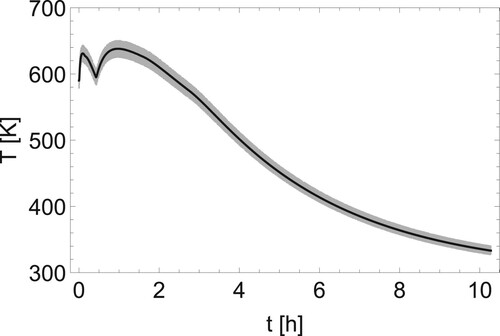
Presentation of results is completed by a couple of figures. In Figure 2, there is shown the reconstructed distribution of temperature, calculated for the cycle of measurements noised by 2% error and taken at every 1 s, plotted in four successive moments of the solidification process. We may observe in the figure the occurrence and development of the air gap together with the monotonic decrease of temperature in the cast and in the mould. We can also see that the temperature is lower in the successive moments of the solidification process. Whereas in Figure 3 the distribution of temperature, obtained for the same set of data, is compared with the cloud of dots representing the measurement values. We may see that the reconstructed line of temperature fits well into the measured values. The shape of the curve illustrates the double change of the boundary condition (14(14) $\begin{array}{rl}& -k_m\frac{\mathrm{\partial }{T}_m(b,t)}{\mathrm{\partial }x}=h(T_m(b,t)-T_{\mathrm{\infty }}),\end{array}$(14) ), represented by the double change of reconstructed value of heat transfer coefficient h. When coefficient h takes its third value $h_3$, which is the lowest, less heat is taken from the cast region, therefore the temperature increases at first, but after this short increase it starts to decrease, as expected in the solidification process. Similar graphs are obtained for other investigated cases of input data.

Figure 2. Temperature distribution reconstructed for the cycle of measurements noised by 2% error and taken at every 1 s in four moments ($t_1=540s$, $t_1=1080s$, $t_1=10,800s$, $t_1=20,800s$) of the solidification process.

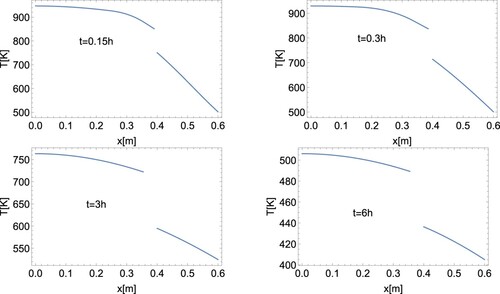
Figure 3. Comparison of the temperature distribution in control point reconstructed for the cycle of measurements noised by 2% error and taken at every 1 s (solid line) with the measurement values (cloud of dots).

The presented numerical experiment was conducted with the aid of computer programs created entirely by the authors (without using any programming libraries), thanks to which the solution programs can be adapted in every step to new conditions. The calculation time was about 18 h.

5. Summarizing conclusions

Aim of this paper was to investigate the procedure of solving the inverse problem of the binary alloy solidification with the macrosegregation and the material shrinkage phenomena taken into account simultaneously. The inverse problem consisted in reconstruction of the following coefficients appearing in the boundary conditions of the model: the heat transfer coefficient and the air gap thermal conductivity, on the ground of temperature measurements taken from the sensor located in the centre of the mould.

The numerical experiment showed that in all 12 cases of input data the coefficients and the temperature were reconstructed with maximal errors almost always lower than the measurement errors and the results obtained in 10 launches gave very comparable results. For most of the considered sets of input data, the maximal relative error of reconstructing four parameters is lower than the input data error, except few cases in which the reconstruction error is slightly higher but not higher than 2.711%, so the output error still keeps the level of the input error. The reconstruction of temperature in the control point is burdened with the maximal relative error almost always lower that 0.1% (except two cases when it takes the values of 0.109% and 0.121%), so the reconstruction of temperature is very good. Moreover, in most of the considered cases, the standard deviation of 10 results, expressed as the per cent of average reconstruction results, does not exceed the value of 1%, and its highest value is equal to 3.634%. The law standard deviation of results, obtained in the repeated calculations, confirms the stability of results. These conclusions lead us to the statement that the proposed procedure may be considered as effective and stable in solving the investigated problem.

Disclosure statement

No potential conflict of interest was reported by the author(s).

References

- Dehghan M, Abbaszadeh M. Proper orthogonal decomposition variational multiscale element free Galerkin (POD-VMEFG) meshless method for solving incompressible Navier-Stokes equation. Comput Methods Appl Mech Eng. 2016;311:856–888.
- Dehghan M, Abbaszadeh M. An upwind local radial basis functions-differential quadrature (RBF-DQ) method with proper orthogonal decomposition (POD) approach for solving compressible Euler equation. Eng Anal Bound Elem. 2018;92:244–256.
- Abbaszadeh M, Dehghan M. Investigation of the Oldroyd model as a generalized incompressible Navier-Stokes equation via the interpolating stabilized element free Galerkin technique. Appl Numer Math. 2020;150:274–294.
- Shirvan KM, Ellahi R, Mirzakhanlari S, et al. Enhancement of heat transfer and heat exchanger effectiveness in a double pipe heat exchanger filled with porous media: numerical simulation and sensitivity analysis of turbulent fluid flow. Appl Therm Eng. 2016;109:761–774.
- Esfahani JA, Akbarzadeh M, Rashidi S, et al. Influences of wavy wall and nanoparticles on entropy generation over heat exchanger plat. Int J Heat Mass Transf. 2017;109:1162–1171.
- Shirvan KM, Mamourian M, Mirzakhanlari S, et al. Numerical investigation of heat exchanger effectiveness in a double pipe heat exchanger filled with nanofluid: A sensitivity analysis by response surface methodology. Powder Technol. 2017;313:99–111.
- Dehghan M, Yousefi SA, Rashedi K. Ritz-Galerkin method for solving an inverse heat conduction problem with a nonlinear source term ia Bernstein multi-scaling functions and cubic B-spline functions. Inverse Probl Sci Eng. 2013;21:500–523.
- Rashedi K, Adibi H, Dehghan M. Determination of space-time-dependent heat source in a parabolic inverse problem via the Ritz-Galerkin technique. Inverse Probl Sci Eng. 2014;22:1077–1108.
- Hetmaniok E. Solution of the inverse problem in solidification of binary alloy by applying the ACO algorithm. Inverse Probl Sci Eng. 2016;24:889–900.
- Reddy SR, Dulikravich GS. Simultaneous determination of spatially varying thermal conductivity and specific heat using boundary temperature measurements. Inverse Probl Sci Eng. 2019;27:1635–1649.
- Zielonka A, Hetmaniok E, Słota D. Reconstruction of the boundary condition in the binary alloy solidification problem with the macrosegregation and the material shrinkage phenomena taken into account. Heat Transfer Eng. 2021;42(3/4):308–318.
- Nawrat A, Skorek J. Inverse finite element technique for identification of thermal resistance of gas-gap between the ingot and mould in continuous casting of metals. Inverse Probl Sci Eng. 2004;12(2):141–155.
- Nawrat A, Skorek J, Sachajdak A. Identification of the heat fluxes and thermal resistance on the ingot-mould surface in continuous casting of metals. Inverse Probl Sci Eng. 2009;17(3):399–409.
- Pickering EJ. Macrosegregation in steel ingots: the applicability of modelling and characterisation techniques. ISIJ Int. 2013;53(6):935–949.
- Nadella R, Eskin DG, Du Q, et al. Macrosegregation in direct-chill casting of aluminium alloys. Prog Mater Sci. 2008;53(3):421–480.
- Zielonka A, Hetmaniok E, Słota D. Application of the immune algorithm IRM for solving the inverse problem of metal alloy solidification including the shrinkage phenomenon. Computer Meth Mater Sci. 2018;18(1):1–10.
- Hetmaniok E, Hristov J, Słota D, et al. Identification of the heat transfer coefficient in the two-dimensional model of binary alloy solidification. Heat Mass Transfer. 2017;53(5):1657–1666.
- Mochnacki B. Numerical modeling of solidification process. In: Zhu J, editor, Computational simulations and applications. INTECH; 2011. p. 513–542.
- Mochnacki B, Suchy JS. Simplified models of macrosegregation. J Theor Appl Mech. 2006;44367–379
- Özişik MN. Heat conduction. Wiley: New York; 1993.
- Majchrzak E, Mochnacki B, Mendakiewicz J. Numerical model of binary alloys solidification basing on the one domain approach and the simple macrosegregation models. Arch Metall Mater. 2015;602431–2435.
- Karaboga D, Akay B. A comparative study of artificial bee colony algorithm. Appl Math Comput. 2009;214:108–132.
- Karaboga D, Basturk B. A powerful and efficient algorithm for numerical function optimization: artificial bee colony (ABC) algorithm. J Global Optim. 2007;39:459–471.
- Zielonka A, Hetmaniok E, Słota D. Inverse alloy solidification problem including the material shrinkage phenomenon solved by using the bee algorithm. Int Commun Heat Mass Transf. 2017;87:295–301.
- Ning A-P, Zhang X-Y. Convergence analysis of artificial bee colony algorithm. Kongzhi Yu Juece/Control Decis. 2013;28:1554–1558.
- Zhang P. Research on convergence of artificial bee colony algorithm based on crossover and consistency distribution-good point set. IOP Conference Series: Earth and Environmental Science; Vol. 446, 2020. p. 052007.
- Liu W. A multistrategy optimization improved artificial bee colony algorithm. Scientific World J. 2014;2014:129483.
- Bansal JC, Gopal A, Nagar AK. Analysing convergence, consistency, and trajectory of artificial bee colony algorithm. IEEE Access. 2018;6:73593–73602.
- Jakšić Krüger T, Davidović T, Teodorović D, et al. The bee colony optimization algorithm and its convergence. Int J Bio-Inspired Comput. 2016;8:340–354.
- Bansal JC, Gopal A, Nagar AK. Stability analysis of artificial bee colony optimization algorithm. Swarm Evol Comput. 2018;41:9–19.
- Fainekos GE, Giannakoglou KC. Inverse design of airfoils based on a novel formulation of the ant colony optimization method. Inverse Probl Eng. 2003;11:21–38.
- Carvalho AR, de Campos Velho HF, Stephany S, et al. Fuzzy ant colony optimization for estimating chlorophyll concentration profile in offshore sea water. Inverse Probl Sci Eng. 2008;16:705–715.
- Lobato FS, Steffen Jr V, Silva Neto AJ. Estimation of space-dependent single scattering albedo in a radiative transfer problem using differential evolution. Inverse Probl Sci Eng. 2012;20:1043–1055.
- Tam JH, Ong ZCh., Ismail Z, et al. Inverse identification of elastic properties of composite materials using hybrid GA-ACO-PSO algorithm. Inverse Probl Sci Eng. 2018;26:1432–1463.
- Brociek R, Słota D, Król M, et al. Comparison of mathematical models with fractional derivative for the heat conduction inverse problem based on the measurements of temperature in porous aluminum. Int J Heat Mass Transf. 2019;143:118440.
- Mochnacki B, Suchy JS. Numerical methods in computations of foundry processes. PFTA: Cracow; 1995.
- Ryfa A, Białecki R. Retrieving the heat transfer coefficient for jet impingement from transient temperature measurements. Int J Heat Fluid Flow. 2011;32:1024–1035.