The generalized flexibility matrix method for structural damage detection with incomplete mode shape data

Abstract

Achieving complete data of measured mode shapes is costly during the process of structural dynamic test. This results in a challenge for the damage detection. This paper concentrates on structural damage detection problem with incomplete mode shape data. An efficient method to deal with this problem is proposed. The generalized flexibility matrix (GFM) is employed. By introducing a few new variables and partitioning the involved matrices, a nonnegative linear least square model is derived. Most of the variables in the model are the damage extents of structural elements. Our method does not involve mode shape expansion or reduction technique.

Three numerical examples show that the performance of the proposed method is superior to that of the GFM method combining with mode shape expansion, it is almost the same as that of the GFM approach with complete mode shapes data.

KEYWORDS:

• Damage detection
• generalized flexibility matrix
• incomplete mode shape
• sensitivity
• nonnegative least square

AMS SUBJECT CLASSIFICATIONS:

• 70J10
• 15A29

1. Introduction

Many engineering structures such as bridges, buildings, dams and pipelines support a society’s economic prosperity and quality of life [1]. During their service life cycles, they may be damaged due to the adverse impact of environmental factors. If these damages cannot be found as soon as possible, they will cause the structure to work ineffectively and may lead to a disaster. Thus finding these damages via nondestructive techniques at the earliest possible stage is very important [2]. Over last few decades, some techniques such as wave propagation, impedance change and ultrasonic inspection have been employed [3], and various methods have been proposed for the damage detection [2–8].

Among these detection methods, vibration-based methods have attracted much attention. Engineers and researchers, especially in fields of aerospace and offshore oil, have begun to use vibration-based methods from the late 1970s and early 1980s [9]. As natural frequencies and mode shapes depend on structural parameters, changes in them can be an effective indication of structural deterioration. Vibration-based methods make full use of changes in the frequency-domain modal properties, such as natural frequencies, mode shapes and its curvatures, modal flexibility and its derivatives, modal strain energy and frequency response function [1].

For example, Ghasemi et al. [10] exploited the modal strain energy for damage detection. Their approach is a two-stage method. In the first stage, elements that are most likely damaged are found by the modal strain energy. Then, extents of damaged elements are calculated by a modified genetic algorithm. Ghannadi and Kourehli [11] developed a new objective function and minimized the function by salp swarm algorithm to detect damages in multi-story shear frames. In addition, many other intelligent optimization methods such as moth-flame algorithm, bee colony algorithm and grey wolf algorithm have been applied to structural damage detection problem [12–14]. Shokrani et al. [15] employed mode shape curvatures for damage locations and used them as a vibration feature in conjunction with principal component analysis for the first time. Their method can locate damage under varying environment conditions. Lu et al. [16] utilized hybrid sensitivity matrices for damage detection in axially functionally graded beams. Yan and Ren [17] gave the closed form of the sensitivity of modal flexibility by eigenvalue and eigenvector derivatives, and adopted it to calculate damage locations and extents. Altunışık et al. have concentrated on detecting multiple cracks in beams by vibration measurements, and presented some methods [18–22]. Structural flexibility matrix and its sensitivity are often be used for damage detection. The idea of flexibility matrix methods is that the reduction in stiffness of any element can increase the amount of flexibility. The earlier flexibility method can only find damage locations [23]. Further method can quantify the extent of damage elements by the flexibility matrix [24]. The drawback of the method is that truncating higher-order mode shapes can cause a larger error. To some extent, this disadvantage is overcome by using the generalized flexible matrix (GFM) method which was first defined and used by Li et al. [25]. Their method can greatly reduce the effect of truncating higher-order mode shapes. Compared with the original flexibility matrix method, less number of natural frequencies and corresponding mode shapes is involved. This leads to widespread applications of the GFM [2,26–29].

The main advantage of vibration-based methods is that it can give a global damage assessment and detect damages which are not on the surface of the structure. However, some adverse conditions in structural dynamic test often restrict the application of vibration-based methods. For example, the response is usually measured at a part position of the structure and values at rotation degrees of freedom (DOFs) are difficult to be achieved [30]. This results in the case that the number of available DOFs is less than that of structural DOFs. To deal with this deficiency, a lot of great efforts have been made and some methods have been proposed [31–41]. Two types of methods are often used. One is to utilize measured mode shape components to estimate values at the unmeasured locations, and get vectors that have the same dimension as complete mode shape vectors. This is mode-shape expansion method [38,39]. The other is reduction method. It partitions the mass and stiffness matrices into a set of master and slave DOFs. Then, a coordinate transformation is employed to condense slave DOFs into master DOFs [40,41]. In fact, mode-shape expansion is essentially the reverse of model reduction, and these two types of methods have some similarities [2]. These methods, especially reduction methods, are often utilized by damage detection with incomplete mode shape data [42–46].

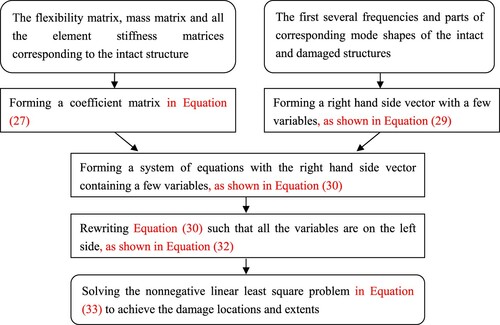
In this paper, the incomplete data is directly employed for the damage detection. Expansion or reduction method is not involved. The flexibility matrix, mass matrix and all the element stiffness matrices corresponding to the intact structure are utilized to form a coefficient matrix. Several low order frequencies and the corresponding incomplete mode shapes are involved to form a right-hand side vector, which contains a few new introduced variables. Thus a system of equations can be got. The variables on the left side of the system are the damage extents of all the elements. Then, the variables in the right side of the system are moved to its left side such that all the variables are on the left side. After that, a new linear system is achieved. The number of variables in the new system is a little more than that of structural elements. Solving this nonnegative linear least square problem, all the damage locations and extents can be obtained. It is different from ways of most detection methods for handing the incomplete mode shape data.

The remainder of the paper is organized as follows. In Section 2, the damage detection problem is formulated and the GFM approach is reviewed. The new method is derived in Section 3. Numerical examples are employed to illustrate the effectiveness of the proposed method in Section 4 and conclusion is drawn in Section 5.

2. Preliminaries

In this section, the damage detection problem is first formulated. Then, the GFM approach is reviewed.

2.1. Problem formulation

In this paper, the damage detection problem is focused on based on following two assumptions.

1. The structural damage only results in a reduction of the structural stiffness, the structural mass remains unchanged.

2. Numbers of DOFs and elements are unchanged after the damage, i.e. numbers of DOFs and elements of the damaged structure equal those of the undamaged structure, respectively.

Under these assumptions, the problem can be formulated as follows [25]. Let ${\mathbf{\text{K}}}_u\in R^{n\times n}$ and ${\mathbf{\text{K}}}_d\in R^{n\times n}$ be global stiffness matrices corresponding to the undamaged and damaged structures, respectively. ${\mathbf{\text{K}}}_{ui}\in R^{n\times n}$ stands for the elemental stiffness matrix corresponding to the $i\text{th}$ element of the undamaged structure. Then, ${\mathbf{\text{K}}}_d$ and ${\mathbf{\text{K}}}_u$ satisfy (1) ${\mathbf{\text{K}}}_d={\mathbf{\text{K}}}_u-\mathrm{\Delta }\mathbf{\text{K}}$(1) where $\mathrm{\Delta }\mathbf{\text{K}}$ is the variation of the global stiffness matrix due to the damage. Owing to the finite element method, ΔK is the sum of changes of some elemental stiffness matrices, i.e. (2) $\mathbf{\Delta }\mathbf{\text{K}}=\sum _{i=1}^m{\alpha }_i{\mathbf{\text{K}}}_{ui}$(2) where $m$ is the number of structural elements, $0\le {\alpha }_i\le 1$ is the damage extent of the $i\text{th}$ element $(i=1,2,\dots ,m)$, ${\alpha }_i=0$ indicates that the $i\text{th}$ element is intact. Due to the existence of measurement noise, small ${\alpha }_i$ cannot show that the $i\text{th}$ element is damaged. In this paper, the $i\text{th}$ element is deemed to be damage only if ${\alpha }_i\ge 0.05$ [25]. The aim of structural damage detection is to find all the damage locations and extents, i.e. calculate ${\alpha }_i$ $(i=1,2,\dots ,m)$ by fully using the measured information.

2.2. The GFM approach

In 2010, Li et al. [25] first proposed the GFM approach. Their method is reviewed in the following.

Substituting Equation (2) into Equation (1) and differentiating with respect to ${\alpha }_i$ yield (3) $\frac{\mathrm{\partial }{\mathbf{\text{K}}}_d}{\mathrm{\partial }{\alpha }_i}=-{\mathbf{\text{K}}}_{ui}$(3)

Let ${\mathbf{\text{F}}}_d\in R^{n\times n}$ be the flexibility matrix of the damaged structure, i.e. (4) ${\mathbf{\text{F}}}_d{\mathbf{\text{K}}}_d=\mathbf{\text{I}}$(4) where $\mathbf{\text{I}}$ is the identity matrix of order $n$. Differentiating Equation (4) with respect to ${\alpha }_i$, we have (5) $\frac{\mathrm{\partial }{\mathbf{\text{F}}}_d}{\mathrm{\partial }{\alpha }_i}{\mathbf{\text{K}}}_d+{\mathbf{\text{F}}}_d\frac{\mathrm{\partial }{\mathbf{\text{K}}}_d}{\mathrm{\partial }{\alpha }_i}=0$(5)

Post-multiplying Equation (5) by ${\mathbf{\text{F}}}_d$ and substituting Equation (3) into it, we get the following equation: (6) $\frac{\mathrm{\partial }{\mathbf{\text{F}}}_d}{\mathrm{\partial }{\alpha }_i}={\mathbf{\text{F}}}_d{\mathbf{\text{K}}}_{ui}{\mathbf{\text{F}}}_d$(6)

Based on the mode shape normalization with respect to the mass matrix, the GFM is introduced. Its definition is given as follows: (7) ${\mathbf{\text{f}}}_d^g(\alpha )={\mathbf{\text{F}}}_d(\mathbf{\text{M}}{\mathbf{\text{F}}}_d{)}^l={\mathbf{\Phi }}_d{\mathbf{\Lambda }}_d^{-1}{\mathbf{\Phi }}_d^{\text{T}}(\mathbf{\text{M}}{\mathbf{\Phi }}_d{\mathbf{\Lambda }}_d^{-1}{\mathbf{\Phi }}_d^{\text{T}}{)}^l={\mathbf{\Phi }}_d{\mathbf{\Lambda }}_d^{-1-l}{\mathbf{\Phi }}_d^{\text{T}}$(7) where $\mathbf{\text{M}}$ is the mass matrix, it remains unchanged before and after the damage, ${\mathbf{\Phi }}_d$ and ${\mathbf{\Lambda }}_d$ are the mode shape matrix and diagonal matrix of natural frequency squared corresponding to the damaged structure, respectively. It can be observed from Equation (7) that a larger $l$ can cause a reduced contribution of higher-order modes. For $l=0$, Equation (7) gives the original flexibility matrix, i.e. ${\mathbf{\text{F}}}_d={\mathbf{\Phi }}_d{\mathbf{\Lambda }}_d^{-1}{\mathbf{\Phi }}_d^{\text{T}}$. For $l=1$, Equation (7) provides the following GFM: (8) ${\mathbf{\text{f}}}_d^g(\alpha )={\mathbf{\text{F}}}_d\mathbf{\text{M}}{\mathbf{\text{F}}}_d={\mathbf{\Phi }}_d{\mathbf{\Lambda }}_d^{-1}{\mathbf{\Phi }}_d^{\text{T}}\mathbf{\text{M}}{\mathbf{\Phi }}_d{\mathbf{\Lambda }}_d^{-1}{\mathbf{\Phi }}_d^{\text{T}}={\mathbf{\Phi }}_d{\mathbf{\Lambda }}_d^{-2}{\mathbf{\Phi }}_d^{\text{T}}$(8)

In this paper, only $l=1$ is employed. Differentiating Equation (8) with respect to ${\alpha }_i$ yields (9) $\frac{\mathrm{\partial }{\mathbf{\text{f}}}_d^g}{\mathrm{\partial }{\alpha }_i}=\frac{\mathrm{\partial }{\mathbf{\text{F}}}_d}{\mathrm{\partial }{\alpha }_i}\mathbf{\text{M}}{\mathbf{\text{F}}}_d+{\mathbf{\text{F}}}_d\mathbf{\text{M}}\frac{\mathrm{\partial }{\mathbf{\text{F}}}_d}{\mathrm{\partial }{\alpha }_i}$(9)

Substituting Equation (6) into Equation (9) and setting ${\alpha }_i=0$ $(i=1,2,\dots ,m)$, we have (10) ${\frac{\mathrm{\partial }{\mathbf{\text{f}}}_d^g}{\mathrm{\partial }{\alpha }_i}|}_{{\alpha }_i=0}={\mathbf{\text{F}}}_u{\mathbf{\text{K}}}_{ui}{\mathbf{\text{F}}}_u\mathbf{\text{M}}{\mathbf{\text{F}}}_u+{\mathbf{\text{F}}}_u\mathbf{\text{M}}{\mathbf{\text{F}}}_u{\mathbf{\text{K}}}_{ui}{\mathbf{\text{F}}}_u$(10) where ${\mathbf{\text{F}}}_u\in R^{n\times n}$ is the flexibility matrix corresponding to the undamaged structure. Using the first-order Taylors series expansion of ${\text{f }}_d^g(\alpha )$, we can get (11) ${\mathbf{\text{f}}}_d^g\approx {\mathbf{\text{f}}}_u^g+\sum _{i=1}^m{\alpha }_i{\frac{\mathrm{\partial }{\mathbf{\text{f}}}_d^g}{\mathrm{\partial }{\alpha }_i}|}_{{\alpha }_i=0}$(11)

From (10) and (11), we have (12) $\mathrm{\Delta }\mathbf{\text{f}}={\mathbf{\text{f}}}_d^g-{\mathbf{\text{f}}}_u^g\approx \sum _{i=1}^m{\alpha }_i({\mathbf{\text{F}}}_u{\mathbf{\text{K}}}_{ui}{\mathbf{\text{F}}}_u\mathbf{\text{M}}{\mathbf{\text{F}}}_u+{\mathbf{\text{F}}}_u\mathbf{\text{M}}{\mathbf{\text{F}}}_u{\mathbf{\text{K}}}_{ui}{\mathbf{\text{F}}}_u)=\sum _{i=1}^m{\alpha }_i{\mathbf{\text{C}}}_i$(12) where ${\mathbf{\text{f}}}_u^g={\mathbf{\text{f}}}_d^g(\mathbf{0})={\mathbf{\text{F}}}_u\mathbf{\text{M}}{\mathbf{\text{F}}}_u$, $\mathrm{\Delta }\mathbf{\text{f}}$ is the variation of the GFM, and (13) ${\mathbf{\text{C}}}_i={\mathbf{\text{F}}}_u{\mathbf{\text{K}}}_{ui}{\mathbf{\text{F}}}_u\mathbf{\text{M}}{\mathbf{\text{F}}}_u+{\mathbf{\text{F}}}_u\mathbf{\text{M}}{\mathbf{\text{F}}}_u{\mathbf{\text{K}}}_{ui}{\mathbf{\text{F}}}_u(i=1,2,\cdots ,m)$(13)

It can be observed from Equation (8) that if frequencies of structures before and after damage satisfy proper distribution, the GFM can be approximated by using only a few of lower order modes. Thus (14) $\mathrm{\Delta }\mathbf{\text{f}}={\mathbf{\text{F}}}_d\mathbf{\text{M}}{\mathbf{\text{F}}}_d-{\mathbf{\text{F}}}_u\mathbf{\text{M}}{\mathbf{\text{F}}}_u\approx \sum _{j=1}^p\frac{1}{{\omega }_{dj}^4}{\mathbf{\Phi }}_{dj}{\mathbf{\Phi }}_{dj}^{\text{T}}-\sum _{j=1}^p\frac{1}{{\omega }_{uj}^4}{\mathbf{\Phi }}_{uj}{\mathbf{\Phi }}_{uj}^{\text{T}}$(14) where $p$ is the number of involved lower order modes, ${\omega }_{dj}$ and ${\mathbf{\Phi }}_{dj}\in R^n$ are the $j\text{th}$ frequency and the mode shape for the damaged structure, ${\omega }_{uj}$ and ${\mathbf{\Phi }}_{uj}\in R^n$ are the $j\text{th}$ frequency and the mode shape for the undamaged structure. From (12) and (14), we have (15) $\sum _{i=1}^m{\alpha }_i{\mathbf{\text{C}}}_i\approx \sum _{j=1}^p\frac{1}{{\omega }_{dj}^4}{\mathbf{\Phi }}_{dj}{\mathbf{\Phi }}_{dj}^{\text{T}}-\sum _{j=1}^p\frac{1}{{\omega }_{uj}^4}{\mathbf{\Phi }}_{uj}{\mathbf{\Phi }}_{uj}^{\text{T}}$(15) Ignoring the error in (15), a linear system with respect to ${\alpha }_i(i=1,2,\dots ,m)$ can be achieved. Solving this system by the nonnegative least square method [47], both damage locations and extents can be obtained.

3. The damage detection approach using incomplete mode shape data

During the process of the structural dynamic test, it is costly to achieve all the DOFs of the structure. For example, values at rotation DOFs are usually difficult to be measured. In this section, a detection method using incomplete mode shape data is proposed. The method is based on the GFM approach. In practice, it is relatively easy to measure the lowest order frequency and the corresponding mode shape. Thus assume $p=1$ in (15). In this case, (15) can be written as follows: (16) $\sum _{i=1}^m{\alpha }_i{\mathbf{\text{C}}}_i\approx \frac{1}{{\omega }_{d1}^4}{\mathbf{\Phi }}_{d1}{\mathbf{\Phi }}_{d1}^{\text{T}}-\frac{1}{{\omega }_{u1}^4}{\mathbf{\Phi }}_{u1}{\mathbf{\Phi }}_{u1}^{\text{T}}$(16)

For the sake of simplicity, use ${\omega }_d$, ${\omega }_u$, ${\mathbf{\Phi }}_d$ and ${\mathbf{\Phi }}_u$to replace ${\omega }_{d1}$, ${\omega }_{u1}$, ${\mathbf{\Phi }}_{d1}$ and ${\mathbf{\Phi }}_{u1}$, respectively, in the following derivation. Thus (16) can be rewritten as (17) $\sum _{i=1}^m{\alpha }_i{\mathbf{\text{C}}}_i\approx \frac{1}{{\omega }_d^4}{\mathbf{\Phi }}_d{\mathbf{\Phi }}_d^{\text{T}}-\frac{1}{{\omega }_u^4}{\mathbf{\Phi }}_u{\mathbf{\Phi }}_u^{\text{T}}$(17)

Note that the approximate relationship (17) holds only when the mode shapes ${\mathbf{\Phi }}_d$ and ${\mathbf{\Phi }}_u$ satisfy the normalization condition with respect to the mass matrix $\mathbf{\text{M}}$. In practice, ${\mathbf{\text{C}}}_i(i=1,2,\dots ,m)$ (in Equation (13)), ${\omega }_u$ and ${\mathbf{\Phi }}_u$ can be calculated by the information of the undamaged structure. By the dynamic test of the damaged structure, ${\omega }_d$ can be achieved, the corresponding measured mode shape ${\mathbf{\Phi }}_m\in R^n$ is a multiple of ${\mathbf{\Phi }}_d$, i.e. (18) ${\mathbf{\Phi }}_m=t{\mathbf{\Phi }}_d$(18) where $t\in R$. If all the DOFs of the damaged structure are measured, i.e. all the components of ${\mathbf{\Phi }}_m$ are known, ${\mathbf{\Phi }}_d$ can be easily calculated by (19) ${\mathbf{\Phi }}_d=\frac{{\mathbf{\Phi }}_m}{\sqrt{{\mathbf{\Phi }}_m^{\text{T}}\mathbf{\text{M}}{\mathbf{\Phi }}_m}}$(19)

Once ${\mathbf{\Phi }}_d$ is obtained, the GFM approach can be employed for damage detection problem. If only part of DOFs of the damaged structure is measured, i.e. some components of ${\mathbf{\Phi }}_m$ are unknown, ${\mathbf{\Phi }}_d$ cannot be achieved by Equation (19). A new detection method is presented here.

Without loss of generality, suppose all the measured components of ${\mathbf{\Phi }}_m$ are in the front of ${\mathbf{\Phi }}_m$. Partition ${\mathbf{\Phi }}_m$ into the following form: (20) ${\mathbf{\Phi }}_m=\left(\begin{array}{c}{\mathbf{\Phi }}_{mI}\\ {\mathbf{\Phi }}_{mII}\end{array}\right)$(20) where ${\mathbf{\Phi }}_{mI}\in R^s$ is known, ${\mathbf{\Phi }}_{mII}\in R^{n-s}$ is unknown. By a suitable partition of ${\mathbf{\Phi }}_d$, ${\mathbf{\text{C}}}_i(i=1,2,\cdots ,m)$ and ${\mathbf{\Phi }}_u$, we have (21) $\begin{array}{rl}{\mathbf{\Phi }}_d& =\left(\begin{array}{c}{\mathbf{\Phi }}_{dI}\\ {\mathbf{\Phi }}_{dII}\end{array}\right)\end{array}$(21) (22) $\begin{array}{rl}{\mathbf{\text{C}}}_i& =\left(\begin{array}{cc}{\mathbf{\text{N}}}_i& {\mathbf{\text{P}}}_i\\ {\mathbf{\text{Q}}}_i& {\mathbf{\text{U}}}_i\end{array}\right)(i=1,2,\cdots ,m)\end{array}$(22) (23) $\begin{array}{rl}{\mathbf{\Phi }}_u& =\left(\begin{array}{c}{\mathbf{\Phi }}_{uI}\\ {\mathbf{\Phi }}_{uII}\end{array}\right)\end{array}$(23) where ${\mathbf{\Phi }}_{dI},{\mathbf{\Phi }}_{uI}\in R^s$ and ${\mathbf{\text{N}}}_i\in R^{s\times s}(i=1,2,\cdots ,m)$. Substituting Equations (18),(20)–(23) into (17), we have (24) $\sum _{i=1}^m{\alpha }_i\left(\begin{array}{cc}{\mathbf{\text{N}}}_i& {\mathbf{\text{P}}}_i\\ {\mathbf{\text{Q}}}_i& {\mathbf{\text{U}}}_i\end{array}\right)\approx \frac{1}{t^2{\omega }_d^4}\left(\begin{array}{cc}{\mathbf{\Phi }}_{mI}{\mathbf{\Phi }}_{mI}^{\text{T}}& {\mathbf{\Phi }}_{mI}{\mathbf{\Phi }}_{mII}^{\text{T}}\\ {\mathbf{\Phi }}_{mII}{\mathbf{\Phi }}_{mI}^{\text{T}}& {\mathbf{\Phi }}_{mII}{\mathbf{\Phi }}_{mII}^{\text{T}}\end{array}\right)-\frac{1}{{\omega }_u^4}\left(\begin{array}{cc}{\mathbf{\Phi }}_{uI}{\mathbf{\Phi }}_{uI}^{\text{T}}& {\mathbf{\Phi }}_{uI}{\mathbf{\Phi }}_{uII}^{\text{T}}\\ {\mathbf{\Phi }}_{uII}{\mathbf{\Phi }}_{uI}^{\text{T}}& {\mathbf{\Phi }}_{uII}{\mathbf{\Phi }}_{uII}^{\text{T}}\end{array}\right)$(24)

Comparing the left upper corner block in (24) and ignoring the error, the following equation can be obtained (25) $\sum _{i=1}^m{\alpha }_i{\mathbf{\text{N}}}_i=\frac{1}{t^2{\omega }_d^4}{\mathbf{\Phi }}_{mI}{\mathbf{\Phi }}_{mI}^{\text{T}}-\frac{1}{{\omega }_u^4}{\mathbf{\Phi }}_{uI}{\mathbf{\Phi }}_{uI}^{\text{T}}$(25)

By using the vec operation, we have (26) $\sum _{i=1}^m{\alpha }_i\text{vec}({\mathbf{\text{N}}}_i)=\frac{1}{t^2{\omega }_d^4}\text{vec}({\mathbf{\Phi }}_{mI}{\mathbf{\Phi }}_{mI}^{\text{T}})-\frac{1}{{\omega }_u^4}\text{vec}({\mathbf{\Phi }}_{uI}{\mathbf{\Phi }}_{uI}^{\text{T}})$(26) where $\text{vec}(\cdot )$ is a vector obtained by stacking columns of the matrix, for the definition of $\text{vec}(\cdot )$, see Refs. [48,49]. Let (27) $\begin{array}{rl}\mathbf{\text{A}}& =[\text{vec}({\mathbf{\text{N}}}_1),\text{ vec}({\mathbf{\text{N}}}_2),\dots ,\text{ vec}({\mathbf{\text{N}}}_m)]\in R^{s^2\times m}\end{array}$(27) (28) $\begin{array}{rl}\mathit{\alpha }& =({\alpha }_1,{\alpha }_2,\dots ,{\alpha }_m{)}^{\text{T}}\in R^m\end{array}$(28) (29) $\begin{array}{rl}\mathbf{\text{b}}& =\mu \mathbf{\text{h}}-\mathbf{\text{g}}\end{array}$(29) where $\mu =\frac{1}{t^2}>0$, $\mathbf{\text{h}}=\frac{1}{{\omega }_d^4}\text{vec}({\mathbf{\Phi }}_{mI}{\mathbf{\Phi }}_{mI}^{\text{T}})\in R^{s^2}$ and $\mathbf{\text{g}}=\frac{1}{{\omega }_u^4}\text{vec}({\mathbf{\Phi }}_{uI}{\mathbf{\Phi }}_{uI}^{\text{T}})\in R^{s^2}$. Then, Equation (26) can be rewritten as (30) $\mathbf{\text{A}}\alpha =\mathbf{\text{b}}$(30)

Note that besides $\mathit{\alpha }\in R^m$, $\mu >0$ in the right-hand side vector b is also unknown. Thus we can calculate $\mathit{\alpha }$ by taking them together as optimization variables, i.e. (31) $\begin{array}{l}\underset{\mathit{\alpha },\mu }{min}||\mathbf{\text{A}}\alpha -\mu \mathbf{\text{h}}+\mathbf{\text{g}}|{|}_2\\ \text{s}\text{.t}\text{. }{\alpha }_i\ge 0(i=1,2,\cdots ,m)\\ \mu \ge \text{0}\end{array}$(31)

The above optimization problem (31) can be solved by the nonnegative least square method [47]. To be more details, let $\mathbf{\text{B}}=[\mathbf{\text{A}},-\mathbf{\text{h}}]\in R^{s^2\times (m+1)}$, $\mathbf{\text{x}}=[{\mathit{\alpha }}^{\text{T}},\mu {]}^{\text{ T}}\in R^{(m+1)}$. Then, Equation (30) can be rewritten as (32) $\mathbf{\text{Bx}}=-\mathbf{\text{g}}$(32)

Problem (31) is equivalent to the following problem: (33) $\begin{array}{l}\underset{\mathbf{\text{x}}}{min}||\mathbf{\text{Bx}}+\mathbf{\text{g}}|{|}_2\\ \text{s}\text{.t}\text{. }{x}_i\ge 0(i=1,2,\cdots ,m+1)\end{array}$(33)

Once the solution ${\mathbf{\text{x}}}^{\ast }\in R^{(m+1)}$ of problem (33) is achieved, the damage extents of all the elements can be got. They are the first $m$ components of ${\mathbf{\text{x}}}^{\ast }$. The flowchart of the proposed method is presented in Figure 1.

Figure 1. Flowchart of the proposed method.

If a crack in the structure satisfies the two assumptions in Section 2.1, it can be detected and assessed by the proposed method. The study in this paper is based on the work in Ref. [29]. But, they are different. The method in Ref. [29] can only deal with structural damage detection problem with complete mode shape data. Our new method can deal with damage detection problem with incomplete mode shape data. The traditional mode shape expansion or reduction technique is not involved. As shown in the above, incomplete mode shape data is handled by introducing a few new variables and partitioning the involved matrices. The idea of handling incomplete mode shape data in this paper is innovative.

4. Numerical examples

In this section, three examples are presented to show the effectiveness of the proposed method. In these examples, the damages are simulated by reducing the stiffness of specified elements. The measured incomplete mode shape is involved in the damage detection process by Equation (20), it is ${\mathbf{\Phi }}_{mI}$ in the equation.

Example 4.1:

Consider a two-span plane beam structure as shown in Figure 2. The length of the structure is $3.6\text{m}$. The modulus of elasticity and density for the material are $E=3\times {10}^{10}\text{Pa}$ and $\rho =2,500\text{kg/}{\text{m}}^3$, respectively. Geometric constants of every beam element are as follows: length $l=0.15\text{m}$, cross-section area $0.25\text{m}\times 0.25\text{m}$, and second moment of area $I_z=3.26\times {10}^{-4}{\text{m}}^4$. The structure has 24 elements and 25 nodes, and the axial displacement of every node is ignored. Thus every node has 2 DOFs except three constrained nodes. The 2 DOFs are transverse displacement and rotation of each node. Two end nodes of the structure are completely constrained. The constrained node at the middle of the structure has one DOF, i.e. rotation DOF. Thus the total number of DOFs is 45. Two damage cases are studied in this example, as shown in Table 1. In this table and the following Tables 5 and 9, damage extent is the percentage reduction of the stiffness of the damaged element.

Figure 2. A two-span plane beam structure.

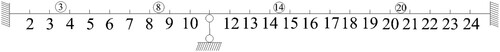
Table 1. Damage cases in Example 4.1.

Damage case	Damaged element(s)	Damage extent
Case 1	Element 8	20%
Case 2	Elements 3, 20	15%
	Element 8	20%
	Element 14	10%

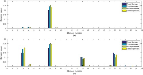
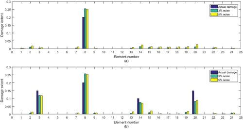
Figure 3 presents the calculated results of the proposed method, the GFM method with mode-shape expansion, and the GFM method. The first two methods use the first frequency and the corresponding translational deflections, while the last method uses the same frequency and the corresponding complete mode shape. It can be seen that the calculated results of these three methods are almost the same. They can exactly find the damaged elements. But, the proposed method and GFM method with mode-shape expansion do not need the values at rotation DOFs of the structure.

Figure 3. Calculated results for damage cases in Table 1: (a) Case 1, (b) Case 2.

Ansys 9.0 is utilized to output the first frequencies and modes corresponding to the intact structure and structures with actual damage and calculated damage by the proposed method. Here, the structure with actual damage means the structure with the damaged element(s) whose damage extent(s) is/are given in Table 1. The structure with calculated damage means the structure with the damaged element(s) whose damage extent(s) is/are determined by the proposed method. The hinge at node 11 is simulated by constraining transverse displacement of this node in Ansys. The rotation of this node is not specified. Table 2 lists the first frequencies corresponding to the intact structure and structures with actual damage and calculated damage for every damage case. It can been seen that for every case, the difference of the two first frequencies is small. The reason for presenting the frequency of the structure is that besides the incomplete mode shape, the proposed method also involves the frequency of the structure. Table 3 gives the relative errors of the first modes of the intact structure and structure with actual damage. Here the relative errors is calculated by the following formula (34) $e=\frac{{||\mathit{\phi }-{\mathit{\phi }}_a||}_2}{{||\mathit{\phi }||}_2}$(34) where $\mathit{\phi }$ and ${\mathit{\phi }}_a$ are the first modes corresponding to the intact structure and structure with actual damage, respectively. Table 4 presents the relative errors of the first modes of the structures with actual damage and calculated damage. Here the relative errors are calculated by the following formula: (35) $\overline{e}=\frac{{||{\mathit{\phi }}_a-{\mathit{\phi }}_c||}_2}{{||{\mathit{\phi }}_a||}_2}$(35) where ${\mathit{\phi }}_c$ is the first mode corresponding to the structure with calculated damage by the proposed method. It can be observed that the relative error is small for every case. This shows that the two first modes are almost the same for every case. Figure 4 presents every component of the difference of the first modes corresponding to the intact structure and the structure with actual damage. Figure 5 gives every component of the difference of the first modes corresponding to the structures with actual damage and calculated damage.

Figure 4. The components of the difference of the first modes corresponding to the intact structure and structure with actual damage in Example 4.1: (a) Case 1, (b) Case 2.

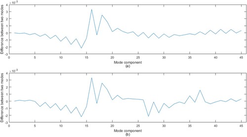
Figure 5. The components of the difference of the first modes corresponding to the structures with actual damage and calculated damage in Example 4.1: (a) Case 1, (b) Case 2.

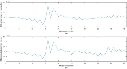
Table 2. The first frequencies of the intact structure and structures with actual damage and calculated damage in Example 4.1.

		Structure with	Structure with
Damage case	Intact structure	actual damage	calculated damage
Case 1	162.76	161.97	161.69
Case 2	162.76	161.40	161.28

Table 3. The relative errors of the first modes of the intact structure and structure with actual damage in Example 4.1.

Damage case	The relative error
Case 1	$1.4936\times {10}^{-2}$
Case 2	$1.7188\times {10}^{-2}$

Table 4. The relative errors of the first modes of the structures with actual damage and calculated damage in Example 4.1.

Damage case	The relative error
Case 1	$5.1686\times {10}^{-3}$
Case 2	$5.8972\times {10}^{-3}$

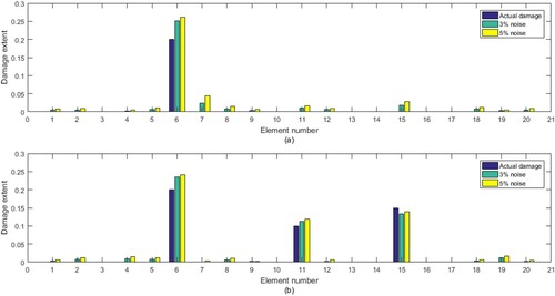
The proposed method has been performed in two random noise environments. The noise level of the natural frequency is $0.5\mathrm{\%}$, and the corresponding deflections are contaminated with $3\mathrm{\%}$ and $5\mathrm{\%}$ random noises, respectively. The noise environments are produced by the following formulas [45,50]: (36a) $\begin{array}{rl}{\overline{\omega }}_d^{\ast }& ={\omega }_d^{\ast }(1+r\rho )\end{array}$(36a) (36b) $\begin{array}{rl}{\overline{\mathit{\Phi }}}_{dj}^{\ast }& ={\mathbf{\Phi }}_{dj}(1+r_j\tilde{\rho }{v}_{max})\end{array}$(36b) where ${\omega }_d^{\ast }$ and ${\overline{\omega }}_d^{\ast }$ are natural frequencies of the damaged structure without and with noise, $r$ and $r_j$ are Gaussian random numbers with mean $0$ and variance $1$, $\rho$ and $\tilde{\rho }$ are the noise levels of the natural frequency and the deflection, respectively. ${\mathbf{\Phi }}_{dj}$ and ${\overline{\mathit{\Phi }}}_{dj}^{\ast }$ are the $j\text{th}$ deflections of the damaged structure without and with noise, and $v_{max}$ is the largest absolute value among all the deflections of the undamaged structure. For every noise environment, 1000 calculations have been done by the proposed method, mean value vectors of these results are given in Figure 6. It can be seen that the proposed method can also work for these two noise environments.

Figure 6. Calculated results for damage cases in Table 1 with two level noises: (a) Case 1, (b) Case 2.

Example 4.2:

Consider a three-span plane beam as shown in Figure 7. The length of the beam is $3.15\text{m}$. The cross section of the beam is square and its size is $0.3\text{m}\times 0.3\text{m}$. The beam is modelled with 21 equal elements of $0.15\text{m}$ in length. The material and geometric parameters of every element are as follows: Young’s modulus $E=3\times {10}^{10}\text{Pa}$, density $\rho =2,500\text{kg/}{\text{m}}^3$, and second moment of area $I_z=6.75\times {10}^{-4}{\text{m}}^4$. The structure has 21 elements and 22 nodes, and all the axial displacements are ignored. Thus every node has 2 DOFs except the four constrained nodes. The DOFs considered per node are a transverse displacement and a rotation. Two end nodes of the structure are completely constrained. The two hinges are at nodes 7 and 17, respectively. Each of them has one DOF, i.e. rotation DOF. Thus the total number of DOFs is 38. Two damage cases are considered, as shown in Table 5.

Figure 7. A three-span plane beam.

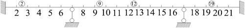
Table 5. Damage cases in Example 4.2.

Damage case	Damaged element(s)	Damage extent
Case 1	Element 2	15%
Case 2	Elements 2, 19	15%
	Element 9	20%
	Element 12	25%

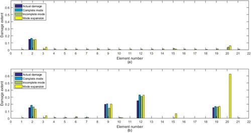
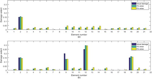
Damage locations and extents are calculated by the proposed method. Only the first frequency and the corresponding translational deflections are used. For comparison, damage locations and extents are also calculated by the GFM method combining with mode-shape expansion technique using the above frequency and translational deflections. In addition, they are calculated by the GFM method using the above frequency and the corresponding complete mode shape. All these calculated results are shown in Figure 8. It can be seen that all these methods can find the damaged elements. But, misjudgments are produced by the GFM method with mode-shape expansion. The calculated results of the proposed method and GFM method using the complete mode shape are almost the same. But the proposed method does not require the values at rotation DOFs of the structure.

Figure 8. Calculated results for damage cases in Table 5: (a) Case 1, (b) Case 2.

Ansys 9.0 is employed to provide the first frequencies and modes corresponding to the intact structure and structures with actual damage and calculated damage by our method. Table 6 presents the lowest frequencies corresponding to the structures with actual damage and calculated damage for every damage case. It can been seen that for the single damage case, the first frequencies are the same. For the multiple damages case, the first frequencies are a little different. Table 7 lists the relative errors of the first modes of the intact structure and structure with actual damage. Table 8 gives the relative errors of the first modes of the structures with actual damage and calculated damage. The formulas for computing relative errors are given in Equations (34) and (35). From Table 8, it can be seen that both of the relative errors are small. This indicates that the two first modes are almost the same for every case. Figure 9 gives every component of the difference of the first modes corresponding to the intact structure and structure with actual damage. Figure 10 lists every component of the difference of the first modes corresponding to the structures with actual damage and calculated damage by the proposed method.

Figure 9. The components of the difference of the first modes corresponding to the intact structure and structure with actual damage in Example 4.2: (a) Case 1, (b) Case 2.

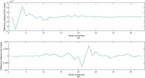
Figure 10. The components of the difference of the first modes corresponding to the structures with actual damage and calculated damage in Example 4.2: (a) Case 1, (b) Case 2.

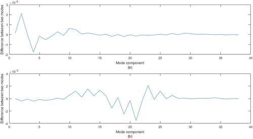
Table 6. The first frequencies of the intact structure and structures with actual damage and calculated damage in Example 4.2.

		Structure with	Structure with
Damage case	Intact structure	actual damage	calculated damage
Case 1	336.12	336.04	336.04
Case 2	336.12	327.98	326.05

Table 7. The relative errors of the first modes of the intact structure and structure with actual damage in Example 4.2.

Damage case	The relative error
Case 1	$1.7999\times {10}^{-3}$
Case 2	$2.9430\times {10}^{-2}$

Table 8. The relative errors of the first modes of the structures with actual damage and calculated damage in Example 4.2.

Damage case	The relative error
Case 1	$7.2147\times {10}^{-5}$
Case 2	$1.4218\times {10}^{-2}$

The proposed method has been carried out in two random noise environments. The method of imposing the noise and levels are the same as those in Example 4.1, as given in Equation (36). For every noise environment, 1000 calculations have been performed, mean value vectors of these results are listed in Figure 11. It can be seen that the proposed method can also exactly find the damaged elements for these two noise environments.

Figure 11. Calculated results for damage cases in Table 5 with two level noises: (a) Case 1, (b) Case 2.

Example 4.3:

Consider a plane truss structure as shown in Figure 12. The length and height of the structure are $10\text{m}$ and $2\text{m}$. The modulus of elasticity and density for the material are $E=2\times {10}^{11}Pa$ and $\rho =7800\text{kg/}{\text{m}}^3$, respectively. The structure is discretized into a finite element model with 20 elements and 10 nodes. Every node has 2 DOFs except the 2 constrainted nodes. The 2 DOFs include the horizontal and vertical displacements of each node. Two supported nodes are completely constrained. Thus the total number of DOFs of the structure is 16. The cross-sectional areas of all elements are $5\times {10}^{-3}{\text{m}}^2$. Two damage cases are considered, as shown in Table 9.

Figure 13 presents the calculated results of the proposed method, the GFM method with mode-shape expansion, and the GFM method. The first two methods use the first frequency and the corresponding vertical deflections, while the last method uses the same frequency and the corresponding complete mode shape. It can be seen that for the single damage case, the calculated results of these three methods are almost the same. They can exactly find the unique damaged element. For the multiple damages case, the proposed method and GFM method work well, while several misjudgments are produced and a damaged element is missed by the GFM method with mode-shape expansion.

Figure 12. A plane truss structure.

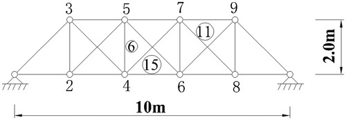
Figure 13. Calculated results for damage cases in Table 9: (a) Case 1, (b) Case 2.

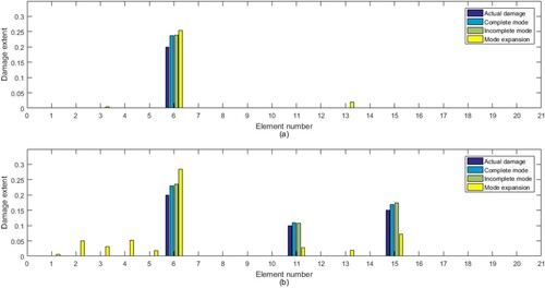
Table 9. Damage cases in Example 4.3.

Damage case	Damaged element(s)	Damage extent
Case 1	Element 6	20%
Case 2	Element 6	20%
	Element 11	10%
	Element 15	15%

Ansys 9.0 is utilized to provide the first frequencies and modes corresponding to the intact structure and structures with actual damage and calculated damage by our method. Table 10 presents the first frequencies corresponding to the intact structure and structures with actual damage and calculated damage for every damage case. Table 11 provides the relative error of the first modes corresponding to the intact structure and structure with actual damage. Table 12 lists the relative error of the first modes corresponding to the structures with actual damage and calculated damage by the proposed method. It can been observed that for every case, the differences of the two first frequencies and modes are very small. Figure 14 gives every component of the difference of the first modes corresponding to the intact structure and the structure with actual damage. Figure 15 exhibits every component of the difference of the first modes corresponding to the structures with actual damage and calculated damage.

Figure 14. The components of the difference of the first modes corresponding to the intact structure and structure with actual damage in Example 4.3: (a) Case 1, (b) Case 2.

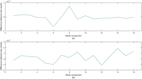
Figure 15. The components of the difference of the first modes corresponding to the structures with actual damage and calculated damage in Example 4.3: (a) Case 1, (b) Case 2.

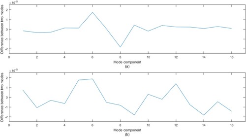
Table 10. The first frequencies of the intact structure and structures with actual damage and calculated damage in Example 4.3.

		Structure with	Structure with
Damage case	Intact structure	actual damage	calculated damage
Case 1	49.008	48.990	48.986
Case 2	49.008	48.845	48.823

Table 11. The relative errors of the first modes of the intact structure and structure with actual damage in Example 4.3.

Damage case	The relative error
Case 1	$1.5693\times {10}^{-3}$
Case 2	$4.8171\times {10}^{-3}$

Table 12. The relative errors of the first modes of the structures with actual damage and calculated damage in Example 4.3.

Damage case	The relative error
Case 1	$3.7963\times {10}^{-4}$
Case 2	$6.5530\times {10}^{-4}$

The proposed method has been carried out in two random noise environments. The way about how to impose the noise are the same as those in Example 4.1, see the corresponding part of Example 4.1. Figure 16 presents the results with two different noise levels. It can be seen that the proposed method can work well for these two noise environments.

Figure 16. Calculated results for damage cases in Table 9 with two level noises: (a) Case 1, (b) Case 2.

From the above three examples, it can be observed that for the single damage case, the proposed method, the GFM method with mode-shape expansion, and the GFM method can find the unique damaged element. But, the GFM method with mode-shape expansion may produce a few misjudgments. For the multiple damages case, the proposed method and GFM method can exactly find the damaged elements. The GFM method with mode-shape expansion can produce some misjudgements and miss the a few damaged elements. Thus the performances of the proposed method and GFM method are superior to that of the GFM method with mode-shape expansion. However, the GFM method needs the first frequency and the corresponding complete mode shape, our method only involves the first frequency and the corresponding incomplete mode shape data.

5. Conclusion

A new damage detection method for incomplete mode shape data is presented. Differing from ways of most detection methods for handling incomplete data, expansion or reduction method is not involved. The proposed method makes use of the GFM and the partition of the involved matrices. A nonnegative least square model is established. The number of variables in the model is a little more than that of structural elements. Numerical examples show that the proposed method is superior to the GFM method combining with mode-shape expansion technique. It can exactly find the damaged elements, both for the single damage case and multiple damages case. The proposed method can obtain almost the same results as those of GFM method. But, the GFM method requires several low-order frequencies and the corresponding complete mode shapes, our method does not require complete mode shapes. More importantly, the idea for handling incomplete mode shape data in this paper can be applied to other detection approaches.

Although the proposed method does not require the complete mode shapes, but some components of the mode shapes are involved. As we all know, the measurement error of mode shape is larger than that of frequency in the process of the structural dynamic test. This limits the application of the method to some extent.

Disclosure statement

No potential conflict of interest was reported by the author(s).

Additional information

Funding

The work was supported by the Natural Science Foundation of China [Grant numbers 11672118 and 11401463] and the Sun Yat-sen University Research Grant for Youth Scholars.

References

- Feng DM, Feng MQ. Computer vision for SHM of civil infrastructure: from dynamic response measurement to damage detection—a review. Eng Struct. 2018;156:105–117.
- Li J, Li ZG, Zhong HX, et al. Structural damage detection using generalized flexibility matrix and changes in natural frequencies. AIAA J. 2012;50(5):1072–1078.
- Palacz M. Spectral methods for modelling of wave propagation in structures in terms of damage detection—a review. Appl Sci. 2018;8(7):1124.
- Smith CB, Hernandez EM. Detection of spatially sparse damage using impulse response sensitivity and LASSO regularization. Inverse Probl Sci Eng. 2019;27(1):1–16.
- Stepinski T, Uhl T, Staszewski W. Advanced structural damage detection: from theory to engineering applications. Chichester: John Wiley & Sons; 2013.
- Zhang C, Gao YW, Huang JP, et al. Damage identification in bridge structures subject to moving vehicle based on extended Kalman filter with l1-norm regularization. Inverse Probl Sci Eng. 2020;28(2):144–174.
- Koh CG, Perry MJ. Structural identification and damage detection using genetic algorithms. London: Taylor & Francis Group; 2010.
- Alexandrino PDL, Gomes GF, Cunha SS. A robust optimization for damage detection using multiobjective genetic algorithm neural network and fuzzy decision making. Inverse Probl Sci Eng. 2020;28(1):21–46.
- Carden EP, Fanning P. Vibration based condition monitoring: a review. Struct Health Monit. 2004;3:355–377.
- Ghasemi MR, Nobahari M, Shabakhty N. Enhanced optimization-based structural damage detection method using modal strain energy and modal frequencies. Eng Comput. 2018;34(3):637–647.
- Ghannadi P, Kourehli SS. Model updating and damage detection in multi-story shear frames using salp swarm algorithm. Earthq Struct. 2019;17:63–73.
- Ghannadi P, Kourehli SS. Multiverse optimizer for structural damage detection: numerical study and experimental validation. Struct Des Tall Spec Build. 2020;29:e1777.
- Ghannadi P, Kourehli SS. Structural damage detection based on MAC flexibility and frequency using moth-flame algorithm. Struct Eng Mech. 2019;70:649–659.
- Ding ZH, Fu KS, Deng W, et al. A modified artificial Bee colony algorithm for structural damage identification under varying temperature based on a novel objective function. Appl Math Model. 2020;88:122–141.
- Shokrani Y, Dertimanis VK, Chatzi EN, et al. On the use of mode shape curvatures for damage localization under varying environmental conditions. Struct Control Health Monit. 2018;25(4):e2132.
- Lu ZR, Lin XX, Chen YM, et al. Hybrid sensitivity matrix for damage identification in axially functionally graded beams. Appl Math Model. 2017;41:604–617.
- Yan WJ, Ren WX. Closed-form modal flexibility sensitivity and its application to structural damage detection without modal truncation error. J Vib Control. 2014;20(12):1816–1830.
- Altunışık AC, Okur FY, Karaca S, et al. Vibration-based damage detection in beam structures with multiple cracks: modal curvature vs. modal flexibility methods. Nondestr Test Eval. 2019;34:33–53.
- Altunışık AC, Okur FY, Kahya V. Automated model updating of multiple cracked cantilever beams for damage detection. J Constr Steel Res. 2017;138:499–512.
- Altunışık AC, Okur FY, Kahya V. Modal parameter identification and vibration based damage detection of a multiple cracked cantilever beam. Eng Fail Anal. 2017;79:154–170.
- Altunışık AC, Okur FY, Kahya V. Structural identification of a cantilever beam with multiple cracks: modeling and validation. Int J Mech Sci. 2017;130:74–89.
- Kahya V, Karaca S, Okur FY, et al. Damage localization in laminated composite beams with multiple edge cracks based on vibration measurements. Iran J Sci Tech Trans Civ Eng. 2020;45:74–87. https://doi.org/https://doi.org/10.1007/s40996-020-00393-x.
- Pandey AK, Biswas M. Damage detection in structures using changes in flexibility. J Sound Vib. 1994;169(1):3–17.
- Yang QW, Liu JK. Damage identification by the eigenparameter decomposition of structural flexibility change. Int J Numer Methods Eng. 2009;78(4):444–459.
- Li J, Wu BS, Zeng QC, et al. A generalized flexibility matrix based approach for structural damage detection. J Sound Vib. 2010;329(22):4583–4587.
- Ashory MR, Masoumi M, Jamshidi E, et al. Using continuous wavelet transform of generalized flexibility matrix in damage identification. J Vibroeng. 2013;15:512–519.
- Masoumi M, Jamshidi E, Bamdad M. Application of generalized flexibility matrix in damage identification using imperialist competitive algorithm. J Civil Eng KSCE. 2015;19(4):994–1001.
- Katebi L, Tehranizadeh M, Mohammadgholibeyki N. A generalized flexibility matrix-based model updating method for damage detection of plane truss and frame structures. J Civil Struct Health Monit. 2018;8(2):301–314.
- Liu HF, Li ZG. An improved generalized flexibility matrix approach for structural damage detection. Inverse Probl Sci Eng. 2020;28(6):877–893.
- Liu FS, Chen WW, Wang WY. An expansion method dealing with spatial incompleteness of measured mode shapes of beam structures. Appl Math Inf Sci. 2014;8(2):651–656.
- Ghannadi P, Kourehli SS. An effective method for damage assessment based on limited measured locations in skeletal structures. Adv Struct Eng. 2020;24(1):183–195. https://doi.org/https://doi.org/10.1177/1369433220947193.
- Ghannadi P, Kourehli SS, Noori M, et al. Efficiency of grey wolf optimization algorithm for damage detection of skeletal structures via expanded mode shapes. Adv Struct Eng. 2020;23(13):2850–2865.
- Ghannadi P, Kourehli SS. Data-driven method of damage detection using sparse sensors installation by SEREPa. J Civ Struct Health Monit. 2019;9(4):459–475.
- Kourehli SS. Prediction of unmeasured mode shapes and structural damage detection using least squares support vector machine. Struct Monit Maint. 2018;5:379–390.
- Ghannadi P, Kourehli SS. Investigation of the accuracy of different finite element model reduction techniques. Struct Monit Maint. 2018;5:417–428.
- Arefi SL, Gholizad A. Damage identification of structures by reduction of dynamic matrices using the modified modal strain energy method. Struct Monit Maint. 2020;7:125–147.
- Arefi SL, Gholizad A, Seyedpoor SM. A modified index for damage detection of structures using improved reduction system method. Smart Struct Syst. 2020;25:1–22.
- Levine-West M, Milman M, Kissil A. Mode shape expansion techniques for prediction – experimental evaluation. AIAA J. 1996;34(4):821–829.
- Liu FS. Direct mode-shape expansion of a spatially incomplete measured mode by a hybrid-vector modification. J Sound Vib. 2011;330(18–19):4633–4645.
- Guyan RJ. Reduction of stiffness and mass matrices. AIAA J. 1965;3(2):380–380.
- Friswell MI, Mottershead JE. Finite element model updating in structural dynamics. Alphen aan den Rijn: Wolters Kluwer; 1995.
- Au FTK, Cheng YS, Tham LG, et al. Structural damage detection based on a micro-genetic algorithm using incomplete and noisy modal test data. J Sound Vib. 2003;259(5):1081–1094.
- Li HJ, Wang JR, Hu SLJ. Using incomplete modal data for damage detection in offshore jacket structures. Ocean Eng. 2008;35(17–18):1793–1799.
- Hosseinzadeh AZ, Amiri GG, Razzaghi SAS, et al. Structural damage detection using sparse sensors installation by optimization procedure based on the modal flexibility matrix. J Sound Vib. 2016;381:65–82.
- Shahri AHH, Ghorbani-Tanha AK. Damage detection via closed-form sensitivity matrix of modal kinetic energy change ratio. J Sound Vib. 2017;401:268–281.
- Yin T, Jiang QH, Yuen KV. Vibration-based damage detection for structural connections using incomplete modal data by Bayesian approach and model reduction technique. Eng Struct. 2017;132:260–277.
- Lawson CL, Hanson RJ. Solving least square problems. Philadelphia: SIAM; 1995.
- Horn RA, Johnson CR. Topics in matrix analysis. Cambridge: Cambridge University Press; 1991.
- Golub GH, Van Loan CF. Matrix computations. 4th ed. Baltimore: The Johns Hopkins University Press; 2013.
- Shi ZY, Law SS, Zhang LM. Structural damage detection from modal strain energy change. J Eng Mech ASCE. 2000;126(12):1216–1223.