Unknown source identification problem for space-time fractional diffusion equation: optimal error bound analysis and regularization method

Abstract

In this paper, the problem of unknown source identification for the space-time fractional diffusion equation is studied. In this equation, the time fractional derivative used is a new fractional derivative, namely, Caputo-Fabrizio fractional derivative. We have illustrated that this problem is an ill-posed problem. Under the assumption of a priori bound, we obtain the optimal error bound analysis of the problem under the source condition. Moreover, we use a modified quasi-boundary regularization method and Landweber iterative regularization method to solve this ill-posed problem. Based on a priori and a posteriori regularization parameter selection rules, the corresponding convergence error estimates of the two regularization methods are obtained, respectively. Compared with the modified quasi-boundary regularization method, the convergence error estimate of Landweber iterative regularization method is order-optimal. Finally, the advantages, stability and effectiveness of the two regularization methods are illustrated by examples with different properties.

Keywords:

• Inverse problem
• Caputo-Fabrizio fractional derivative
• space-time fractional diffusion equation
• optimal error bound
• unknown source identification

2010 Mathematics Subject Classifications:

• 35R25
• 47A52
• 35R30

1. Introduction

In the past few decades, the fractional diffusion equation was attracted much attention from many scholars. For fractional derivatives, different fractional derivatives are used in different fractional diffusion equations. There are many kinds of fractional derivatives, such as Caputo fractional derivative, Riesz fractional derivative, Grunwald Letnikov fractional derivative, Riemann-Liouville fractional derivative and so on. In order to solve the problem of singular kernel of fractional derivative, Caputo and Fabrizio developed a new fractional derivative with smooth kernel, called fractional Caputo-Fabrizio derivative (FCFD) in 2015 [1]. It could describe the inhomogeneity of materials and the fluctuation of different scales. About the direct problem of fractional Caputo-Fabrizio derivative (FCFD) equation, there are a lot of researches results. Losada and Nieto studied some properties of FCFD [2]. The following were some well-posed problems of differential equations with FCFD studied by some scholars, such as Cauchy problem, uniqueness of solutions, existence of solutions, etc. In [3], the authors studied the Cauchy problem of the space-time fractional diffusion equation, where the time fractional derivative was a new fractional derivative Caputo-Fabrizio fractional derivative. Firstly, the expression of the solution of the linear diffusion equation was obtained by Laplace transform, proving the uniqueness of the solution. Secondly, under the global Lipschitz assumption, the regularity of weak solutions in linear and nonlinear cases was studied, and the existence of local mild solutions was given under the local Lipschitz assumption. In [4], Xiangcheng Zheng and Hong Wang studied a class of nonlinear with variable order FCFD fractional order ordinary differential equation. It was proved that the problem was well-posed. The method was further extended and the well-posedness results of linear partial differential equations were proved. In [5], Al-Salti considered a class of boundary value problem for time fractional heat conduction equations with FCFD. The existence and uniqueness of the solution were proved by the method of separation of variables and the initial value problem of fractional order differential. The Caputo-Fabrizio fractional heat conduction equation was transformed into Volterra integral equation to solve. Different solutions were given for different parameters. As a differential operator, FCFD had a wide range of applications. It was applied to many models in many fields, such as dynamic system, biomedicine, electro magnetics and so on. In [6], Baleanu proposed a new FCFD model that included an index kernel. The uniqueness of the solution was proved. The convergence was analysed. Through numerical experiments, it was proved that the new fractional order model was better than the integer order model with ordinary time derivative. In [7], Al-khedhairi proposed a financial model with non-smooth FCFD. The existence and uniqueness of the solution of the model was proved. The local stability was analysed and the key dynamic properties of the model were studied. In [8], the authors consider the case of linear fractional differential equations: ${}_{CF}{D}_{a,t}^{\alpha }u\left(t\right)-\lambda u\left(t\right)=f\left(t\right),t\ge a,$where $1<\alpha <2$, $a\in (-\mathrm{\infty },t)$ and ${}_{CF}{D}_{a,t}^{\alpha }\nu \left(t\right)=\frac{1}{2-\alpha }{\int }_a^t\exp (-\frac{\alpha }{1-\alpha }(t-s\left)\right)\frac{{\mathrm{\partial }}^2\nu \left(s\right)}{\mathrm{\partial }{s}^2}\mathrm{d}s$, and studied the explicit form of the general solution of fixed point. On this basis, the uniqueness of the solution to the initial value problem of nonlinear differential equations was studied. In [9,10], the form of numerical solution and algorithm of differential equations with FCFD were mainly studied. In [9], the authors introduced the second-order scheme for the distribution of particle anomalous motion function and derived a spatial fractional diffusion equation with time FCFD based on a continuous time random walk model ${}_0^{CF}{D}_t^{\gamma }u(x,y,t)=\frac{{\mathrm{\partial }}^{\alpha }u(x,y,t)}{\mathrm{\partial }|x{|}^{\alpha }}+\frac{{\mathrm{\partial }}^{\text{β}}u(x,y,t)}{\mathrm{\partial }|y{|}^{\text{β}}}+f(x,y,t).$It was shown that the scheme was unconditionally stable. Through theoretical proof and numerical verification, the stability of the scheme was proved and the optimal estimation was obtained. In [10], based on the new fractional derivative FCFD, the authors introduced the Crank-Nicolson difference scheme for solving the fractional Cattaneo equation: $\frac{\mathrm{\partial }u(x,t)}{\mathrm{\partial }t}+\frac{{\mathrm{\partial }}^{\alpha }u(x,t)}{\mathrm{\partial }{t}^{\alpha }}=\frac{{\mathrm{\partial }}^{2}u(x,t)}{\mathrm{\partial }{x}^2}+f(x,t),$where $(x,t)=[0,L]\times [0,T]$, $1<\alpha <2$, $f\in C[0,T]$. On the basis of uniform division, a priori estimate of discrete $L^{\mathrm{\infty }}\left(L^2\right)$ error with optimal order of convergence speed $O({\tau }^2+h^2)$ was established. Numerical experiments verified the applicability and accuracy of the format and provide support for theoretical analysis.

In recent years, involved in fractional differential equations, Caputo fractional derivative and Riemann-Liouville fractional derivative are the most common fractional derivatives in the inverse problem literature. Moreover, most fractional differential equations only do fractional operations on time, not spatial fractional order. To our knowledge, so far, few papers have discussed the inverse problem of Caputo-Fabrizio fractional derivative. There is no literature to use the regularization method to deal with the ill-posed problem of differential equations containing Caputo-Fabrizio fractional derivative.

Nowadays, it is a hot topic in the field of inverse problems to deal with ill-posed problems by regularization method. There are many regularization methods to deal with ill-posed problem. In the early days, most scholars used Tikhonov regularization method [11,12] to deal with inverse problems. It is one of the oldest regularization methods. Later, on the basis of Tikhonov regularization method, some scholars studied the modified Tikhonov regularization method [13], the fractional Tikhonov regularization method [14,15] and the simplified Tikhonov regularization method [16]. In dealing with the inverse problem of bounded domain, the regularization methods are as follows: quasi-boundary regularization method [17–19], the truncation regularization method [20,21], a modified quasi-boundary regularization method [22], a mollification regularization method [23], quasi-reversibility regularization method [24,25], Landweber iterative regularization method [26–28], etc. In solving the inverse problem in unbounded domain, the common regularization methods are Fourier truncation regularization method [29–32]. In [33], Liu and Feng considered a backward problem of spatial fractional diffusion equation, and constructed a regularization method based on the improved ‘kernel’ idea, namely the improved kernel method. The modified kernel method can also deal with more ill-posed problem [34–37].

In this paper, we first prove the uniqueness of the solution of problem (1(1) $\left\{\begin{array}{ll}{}_{CF}{D}_{0,t}^{\alpha }u(x,t)+(-L{)}^{s}u(x,t)=f(x\left)q\right(t),& \mathrm{i}\mathrm{n}\mathrm{\Omega }\times (0,T),\\ u(x,t)=0,& \mathrm{o}\mathrm{n}\mathrm{\partial }\mathrm{\Omega }\times (0,T),\\ u(x,0)=\phi \left(x\right),& \mathrm{i}\mathrm{n}\left\{0\right\}\times \mathrm{\Omega },\\ u(x,T)=g\left(x\right),& x\in \mathrm{\Omega },\end{array}\right.$(1) ), and illustrate the ill-posedness of the inverse problem (1(1) $\left\{\begin{array}{ll}{}_{CF}{D}_{0,t}^{\alpha }u(x,t)+(-L{)}^{s}u(x,t)=f(x\left)q\right(t),& \mathrm{i}\mathrm{n}\mathrm{\Omega }\times (0,T),\\ u(x,t)=0,& \mathrm{o}\mathrm{n}\mathrm{\partial }\mathrm{\Omega }\times (0,T),\\ u(x,0)=\phi \left(x\right),& \mathrm{i}\mathrm{n}\left\{0\right\}\times \mathrm{\Omega },\\ u(x,T)=g\left(x\right),& x\in \mathrm{\Omega },\end{array}\right.$(1) ), in other words, the solution does not depend continuously on the measured data. Secondly, we use the modified quasi-boundary regularization method to solve the ill-posed problem (1(1) $\left\{\begin{array}{ll}{}_{CF}{D}_{0,t}^{\alpha }u(x,t)+(-L{)}^{s}u(x,t)=f(x\left)q\right(t),& \mathrm{i}\mathrm{n}\mathrm{\Omega }\times (0,T),\\ u(x,t)=0,& \mathrm{o}\mathrm{n}\mathrm{\partial }\mathrm{\Omega }\times (0,T),\\ u(x,0)=\phi \left(x\right),& \mathrm{i}\mathrm{n}\left\{0\right\}\times \mathrm{\Omega },\\ u(x,T)=g\left(x\right),& x\in \mathrm{\Omega },\end{array}\right.$(1) ). Based on a priori and a posteriori regularization parameter selection rules, we give the convergence error estimates between the exact solution and the regularization solution. However, the convergence error estimates obtained by the modified quasi-boundary regularization method will lead to saturation phenomenon. In addition, we propose a second regularization method, Landweber iterative regularization method, to solve this ill-posed problem. Through the study, we find that the error estimation results obtained by Landweber iterative regularization method will not produce saturation phenomenon, and the convergence error estimates under the a priori and a posteriori regularization parameter choice rules are order optimal.

In this paper, we consider the following problem: (1) $\left\{\begin{array}{ll}{}_{CF}{D}_{0,t}^{\alpha }u(x,t)+(-L{)}^{s}u(x,t)=f(x\left)q\right(t),& \mathrm{i}\mathrm{n}\mathrm{\Omega }\times (0,T),\\ u(x,t)=0,& \mathrm{o}\mathrm{n}\mathrm{\partial }\mathrm{\Omega }\times (0,T),\\ u(x,0)=\phi \left(x\right),& \mathrm{i}\mathrm{n}\left\{0\right\}\times \mathrm{\Omega },\\ u(x,T)=g\left(x\right),& x\in \mathrm{\Omega },\end{array}\right.$(1) where $0<\alpha <1$, $0<s\le 1$, Ω is a bounded domain in ${\mathbb{R}}^d(d=1,2,3)$ with sufficient glossy boundary $\mathrm{\partial }\mathrm{\Omega }$. ${}_{CF}{D}_{0,t}^{\alpha }$ is the Caputo-Fabrizio operator for fractional derivatives of order α which is defined as follows: assume a>0, $\nu \in {\mathbb{H}}^1(0,a)$, and $\alpha \in (0,1)$, for a function with a first derivative ν, its Caputo-Fabrizio fractional derivative is defined as [5]: ${}_{CF}{D}_{0,t}^{\alpha }\nu \left(t\right)=\frac{1}{1-\alpha }{\int }_0^t\exp \left(-\frac{\alpha }{1-\alpha }(t-z)\right)\frac{\mathrm{\partial }\nu \left(z\right)}{\mathrm{\partial }z}\mathrm{d}z,\mathrm{f}\mathrm{o}\mathrm{r}t\ge 0.$In problem (1(1) $\left\{\begin{array}{ll}{}_{CF}{D}_{0,t}^{\alpha }u(x,t)+(-L{)}^{s}u(x,t)=f(x\left)q\right(t),& \mathrm{i}\mathrm{n}\mathrm{\Omega }\times (0,T),\\ u(x,t)=0,& \mathrm{o}\mathrm{n}\mathrm{\partial }\mathrm{\Omega }\times (0,T),\\ u(x,0)=\phi \left(x\right),& \mathrm{i}\mathrm{n}\left\{0\right\}\times \mathrm{\Omega },\\ u(x,T)=g\left(x\right),& x\in \mathrm{\Omega },\end{array}\right.$(1) ), when $f\left(x\right)$ are known, the problem is well-being problem. If $f\left(x\right)$ is unknown, using the additional condition $u(x,T)=g\left(x\right),$ we can get the space-dependent source term $f\left(x\right)$. But in practice, $g\left(x\right)$ can only be obtained by measurement, so there will be errors between the measured data and the exact data.

Assumption 1.1

We assume that the measured data function $g^{\delta }\left(x\right)$ and the exact data function $g\left(x\right)$ satisfy (2) $\parallel g^{\delta }(\cdot )-g(\cdot )\parallel \le \delta ,$(2) where the constant $\delta >0$ represents a noise level and $\parallel \cdot \parallel$ denotes the $L^2\left(\mathrm{\Omega }\right)$ norm.

Definition 1.1

Without loss of generality, admit a family of eigenvalues $0<{\lambda }_1\le {\lambda }_2\le \cdots \le {\lambda }_n\le \cdots ,$ $\underset{n\to \mathrm{\infty }}{lim}{\lambda }_n=+\mathrm{\infty }$, with the function set $\{X_n{\}}_{n=1}^{\mathrm{\infty }}$ constituting an orthonormal basis in space $L^2\left(\mathrm{\Omega }\right)$.

Denote the eigenvalues of the fractional power operators $(-L)$ as ${\lambda }_n$ and the corresponding eigenfunctions as $X_n\left(x\right)\in {\mathbb{H}}^2\left(\mathrm{\Omega }\right)\cap {\mathbb{H}}_0^1\left(\mathrm{\Omega }\right)$, then we can get $\left\{\begin{array}{ll}(-L{)}^s{X}_n(x)={\lambda }_n^s{X}_n(x),& \mathrm{i}\mathrm{n}\mathrm{\Omega },0<s\le 1,\\ X_n\left(x\right)=0,& \mathrm{o}\mathrm{n}\mathrm{\partial }\mathrm{\Omega }.\end{array}\right.$According to the result in [3], the solution of the problem (1(1) $\left\{\begin{array}{ll}{}_{CF}{D}_{0,t}^{\alpha }u(x,t)+(-L{)}^{s}u(x,t)=f(x\left)q\right(t),& \mathrm{i}\mathrm{n}\mathrm{\Omega }\times (0,T),\\ u(x,t)=0,& \mathrm{o}\mathrm{n}\mathrm{\partial }\mathrm{\Omega }\times (0,T),\\ u(x,0)=\phi \left(x\right),& \mathrm{i}\mathrm{n}\left\{0\right\}\times \mathrm{\Omega },\\ u(x,T)=g\left(x\right),& x\in \mathrm{\Omega },\end{array}\right.$(1) ) is (3) $\begin{array}{rl}u(x,t)& =\sum _{n=1}^{\mathrm{\infty }}\left[\frac{1}{1+{\lambda }_n^s(1-\alpha )}\exp \left(\frac{-\alpha {\lambda }_n^{s}t}{1+{\lambda }_n^s(1-\alpha )}\right){\phi }_n\right.\\ & \left.+\frac{f_n}{1+{\lambda }_n^s(1-\alpha )}{\int }_0^{t}q\left(z\right)\exp \left(\frac{\alpha {\lambda }_n^s(z-t)}{1+{\lambda }_n^s(1-\alpha )}\right)\mathrm{d}z\right]X_n\left(x\right)\\ & :=\sum _{n=1}^{\mathrm{\infty }}\left[Q_n\left(t\right){\phi }_n+f_n{\int }_0^{t}q\left(z\right)Q_n(t-z)\mathrm{d}z\right]X_n\left(x\right),\end{array}$(3) where $Q_n\left(t\right)=\frac{1}{1+{\lambda }_n^s(1-\alpha )}\exp \left(\frac{-\alpha {\lambda }_n^{s}t}{1+{\lambda }_n^s(1-\alpha )}\right)$, ${\phi }_n=\left(\phi \right(x),X_n(x\left)\right)$, and $f_n=\left(f\right(x),X_n(x\left)\right)$ are the Fourier coefficients. Applying additional condition $u(x,T)=g\left(x\right)$ and combining with formula (3(3) $\begin{array}{rl}u(x,t)& =\sum _{n=1}^{\mathrm{\infty }}\left[\frac{1}{1+{\lambda }_n^s(1-\alpha )}\exp \left(\frac{-\alpha {\lambda }_n^{s}t}{1+{\lambda }_n^s(1-\alpha )}\right){\phi }_n\right.\\ & \left.+\frac{f_n}{1+{\lambda }_n^s(1-\alpha )}{\int }_0^{t}q\left(z\right)\exp \left(\frac{\alpha {\lambda }_n^s(z-t)}{1+{\lambda }_n^s(1-\alpha )}\right)\mathrm{d}z\right]X_n\left(x\right)\\ & :=\sum _{n=1}^{\mathrm{\infty }}\left[Q_n\left(t\right){\phi }_n+f_n{\int }_0^{t}q\left(z\right)Q_n(t-z)\mathrm{d}z\right]X_n\left(x\right),\end{array}$(3) ), we can get (4) $\begin{array}{rl}g\left(x\right)& =\sum _{n=1}^{\mathrm{\infty }}\left[\frac{1}{1+{\lambda }_n^s(1-\alpha )}\exp \left(\frac{-\alpha {\lambda }_n^{s}T}{1+{\lambda }_n^s(1-\alpha )}\right){\phi }_n\right.\\ & \left.+\frac{f_n}{1+{\lambda }_n^s(1-\alpha )}{\int }_0^{T}q\left(z\right)\exp \left(\frac{\alpha {\lambda }_n^s(z-T)}{1+{\lambda }_n^s(1-\alpha )}\right)\mathrm{d}z\right]X_n\left(x\right)\\ & :=\sum _{n=1}^{\mathrm{\infty }}\left[Q_n\left(T\right){\phi }_n+f_n{\int }_0^{T}q\left(z\right)Q_n(T-z)\mathrm{d}z\right]X_n\left(x\right).\end{array}$(4) Moreover, we have (5) $g_n=Q_n\left(T\right){\phi }_n+f_n{\int }_0^{t}q\left(z\right)Q_n(T-z)\mathrm{d}z,$(5) where $Q_n\left(T\right)=\frac{1}{1+{\lambda }_n^s(1-\alpha )}\exp \left(\frac{-\alpha {\lambda }_n^{s}T}{1+{\lambda }_n^s(1-\alpha )}\right)$, and $g_n=\left(g\right(x),X_n(x\left)\right)$ is the Fourier coefficients.

Let $h\left(x\right)=g\left(x\right)-\sum _{n=1}^{\mathrm{\infty }}{Q}_n\left(T\right){\phi }_n{X}_n\left(x\right)$, then $h_n=g_n-Q_n\left(T\right){\phi }_n.$ Therefore, (4(4) $\begin{array}{rl}g\left(x\right)& =\sum _{n=1}^{\mathrm{\infty }}\left[\frac{1}{1+{\lambda }_n^s(1-\alpha )}\exp \left(\frac{-\alpha {\lambda }_n^{s}T}{1+{\lambda }_n^s(1-\alpha )}\right){\phi }_n\right.\\ & \left.+\frac{f_n}{1+{\lambda }_n^s(1-\alpha )}{\int }_0^{T}q\left(z\right)\exp \left(\frac{\alpha {\lambda }_n^s(z-T)}{1+{\lambda }_n^s(1-\alpha )}\right)\mathrm{d}z\right]X_n\left(x\right)\\ & :=\sum _{n=1}^{\mathrm{\infty }}\left[Q_n\left(T\right){\phi }_n+f_n{\int }_0^{T}q\left(z\right)Q_n(T-z)\mathrm{d}z\right]X_n\left(x\right).\end{array}$(4) ) and (5(5) $g_n=Q_n\left(T\right){\phi }_n+f_n{\int }_0^{t}q\left(z\right)Q_n(T-z)\mathrm{d}z,$(5) ) can be rewritten as (6) $\begin{array}{rl}h\left(x\right)& =\sum _{n=1}^{\mathrm{\infty }}\left[f_n{\int }_0^{T}q\left(z\right)Q_n(T-z)\mathrm{d}z\right]X_n\left(x\right),\end{array}$(6) (7) $\begin{array}{rl}{h}_n& =f_n{\int }_0^{T}q\left(z\right)Q_n(T-z)\mathrm{d}z,\end{array}$(7) where $h_n=\left(h\right(x),X_n(x\left)\right)$ is the Fourier coefficients.

Consequently, we obtain the exact solution of the source term as follows (8) $f\left(x\right)=\sum _{n=1}^{\mathrm{\infty }}\frac{h_n}{{\int }_0^{T}q\left(z\right)Q_n(T-z)\mathrm{d}z}{X}_n\left(x\right).$(8) Due to $h_n=g_n-Q_n\left(T\right){\phi }_n$, then $h_n^{\delta }=g_n^{\delta }-Q_n\left(T\right){\phi }_n$. Consequently, $\begin{array}{rl}{h}_n^{\delta }-h_n& =g_n^{\delta }-Q_n\left(T\right){\phi }_n-g_n+Q_n\left(T\right){\phi }_n\\ & =g_n^{\delta }-g_n.\end{array}$Therefore, according to (2(2) $\parallel g^{\delta }(\cdot )-g(\cdot )\parallel \le \delta ,$(2) ), we have (9) $\parallel h^{\delta }(\cdot )-h(\cdot )\parallel \le \delta .$(9) The organizational structure of this paper is as follows. In the second section, we analyse the uniqueness of the solution and ill-posedness of the problem (1(1) $\left\{\begin{array}{ll}{}_{CF}{D}_{0,t}^{\alpha }u(x,t)+(-L{)}^{s}u(x,t)=f(x\left)q\right(t),& \mathrm{i}\mathrm{n}\mathrm{\Omega }\times (0,T),\\ u(x,t)=0,& \mathrm{o}\mathrm{n}\mathrm{\partial }\mathrm{\Omega }\times (0,T),\\ u(x,0)=\phi \left(x\right),& \mathrm{i}\mathrm{n}\left\{0\right\}\times \mathrm{\Omega },\\ u(x,T)=g\left(x\right),& x\in \mathrm{\Omega },\end{array}\right.$(1) ). In addition, the conditional stability result is also given. In the third section, we first give some preliminary results, and then use these preliminary results to obtain the optimal error bound estimates of the problem (1(1) $\left\{\begin{array}{ll}{}_{CF}{D}_{0,t}^{\alpha }u(x,t)+(-L{)}^{s}u(x,t)=f(x\left)q\right(t),& \mathrm{i}\mathrm{n}\mathrm{\Omega }\times (0,T),\\ u(x,t)=0,& \mathrm{o}\mathrm{n}\mathrm{\partial }\mathrm{\Omega }\times (0,T),\\ u(x,0)=\phi \left(x\right),& \mathrm{i}\mathrm{n}\left\{0\right\}\times \mathrm{\Omega },\\ u(x,T)=g\left(x\right),& x\in \mathrm{\Omega },\end{array}\right.$(1) ). Next, we use the modified quasi-boundary regularization method to solve the inverse problem (1(1) $\left\{\begin{array}{ll}{}_{CF}{D}_{0,t}^{\alpha }u(x,t)+(-L{)}^{s}u(x,t)=f(x\left)q\right(t),& \mathrm{i}\mathrm{n}\mathrm{\Omega }\times (0,T),\\ u(x,t)=0,& \mathrm{o}\mathrm{n}\mathrm{\partial }\mathrm{\Omega }\times (0,T),\\ u(x,0)=\phi \left(x\right),& \mathrm{i}\mathrm{n}\left\{0\right\}\times \mathrm{\Omega },\\ u(x,T)=g\left(x\right),& x\in \mathrm{\Omega },\end{array}\right.$(1) ). In Section 4, we obtain the convergence error estimates between the regularized solution and the exact solution under the a priori and a posteriori regularization parameter selection rules. In Section 5, we present a second regularization method, Landweber iterative regularization method, to deal with this ill-posed problem. In Section 6, we compare the error estimates obtained by two regularization methods for the inverse problem (1(1) $\left\{\begin{array}{ll}{}_{CF}{D}_{0,t}^{\alpha }u(x,t)+(-L{)}^{s}u(x,t)=f(x\left)q\right(t),& \mathrm{i}\mathrm{n}\mathrm{\Omega }\times (0,T),\\ u(x,t)=0,& \mathrm{o}\mathrm{n}\mathrm{\partial }\mathrm{\Omega }\times (0,T),\\ u(x,0)=\phi \left(x\right),& \mathrm{i}\mathrm{n}\left\{0\right\}\times \mathrm{\Omega },\\ u(x,T)=g\left(x\right),& x\in \mathrm{\Omega },\end{array}\right.$(1) ). In Section 7, three numerical examples of different properties are given. In Section 8, we make a brief summary of the whole paper.

2. Conditional stability results, uniqueness and ill-posed analysis for inverse problem (1)

In this section, we mainly discuss uniqueness of solution, the ill-posed analysis and conditional stability of the unknown source identification problem of inverse problem (1(1) $\left\{\begin{array}{ll}{}_{CF}{D}_{0,t}^{\alpha }u(x,t)+(-L{)}^{s}u(x,t)=f(x\left)q\right(t),& \mathrm{i}\mathrm{n}\mathrm{\Omega }\times (0,T),\\ u(x,t)=0,& \mathrm{o}\mathrm{n}\mathrm{\partial }\mathrm{\Omega }\times (0,T),\\ u(x,0)=\phi \left(x\right),& \mathrm{i}\mathrm{n}\left\{0\right\}\times \mathrm{\Omega },\\ u(x,T)=g\left(x\right),& x\in \mathrm{\Omega },\end{array}\right.$(1) ).

Definition 2.1

For any $\gamma >0$ and $0<s\le 1$, defined (10) $D\left(\right(-L^s{)}^{\gamma })=\left\{\varphi \in L^2\left(\mathrm{\Omega }\right)|\sum _{n=1}^{\mathrm{\infty }}\left({\lambda }_n^s{)}^{2\gamma }|\right(\varphi ,X_n){|}^2<\mathrm{\infty }\right\},$(10) where $(\cdot ,\cdot )$ is the inner product in $L^2\left(\mathrm{\Omega }\right)$. Then $D\left(\right(-L^s{)}^{\gamma })$ is a Hilbert space with the norm (11) $\parallel \varphi {\parallel }_{D\left(\right(-L^s{)}^{\gamma })}:={\left(\sum _{n=1}^{\mathrm{\infty }}\left({\lambda }_n^s{)}^{2\gamma }|\right(\varphi ,X_n){|}^2\right)}^{\frac{1}{2}}.$(11)

Some Lemmas and Theorems given below are the results of conditional stability and some conclusions, which can help us analyse the ill-posed of inverse problem (1(1) $\left\{\begin{array}{ll}{}_{CF}{D}_{0,t}^{\alpha }u(x,t)+(-L{)}^{s}u(x,t)=f(x\left)q\right(t),& \mathrm{i}\mathrm{n}\mathrm{\Omega }\times (0,T),\\ u(x,t)=0,& \mathrm{o}\mathrm{n}\mathrm{\partial }\mathrm{\Omega }\times (0,T),\\ u(x,0)=\phi \left(x\right),& \mathrm{i}\mathrm{n}\left\{0\right\}\times \mathrm{\Omega },\\ u(x,T)=g\left(x\right),& x\in \mathrm{\Omega },\end{array}\right.$(1) ). It is applicable to the whole paper.

Lemma 2.1

For any $0<\alpha <1$ and $0<s\le 1$, we obtain (12) $(1+{\lambda }_n^s(1-\alpha \left)\right)\exp \left(\frac{\alpha {\lambda }_n^{s}T}{1+{\lambda }_n^s(1-\alpha )}\right)\le C_0\exp \left(\frac{\alpha T}{1-\alpha }\right){\lambda }_n^s,$(12) where $C_0=max\{\overline{C},\underset{\_}{C}\}.$

Proof.

Due to $\frac{\alpha {\lambda }_n^{s}T}{1+{\lambda }_n^s(1-\alpha )}<\frac{\alpha {\lambda }_n^{s}T}{(1-\alpha ){\lambda }_n^s}=\frac{\alpha T}{1-\alpha }$, according to function $\exp \left(z\right)$ is an increasing function, we can get (13) $\exp \left(\frac{\alpha {\lambda }_n^{s}T}{1+{\lambda }_n^s(1-\alpha )}\right)\le \exp \left(\frac{\alpha T}{1-\alpha }\right).$(13) Combining (13(13) $\exp \left(\frac{\alpha {\lambda }_n^{s}T}{1+{\lambda }_n^s(1-\alpha )}\right)\le \exp \left(\frac{\alpha T}{1-\alpha }\right).$(13) ) and $0<\alpha <1$, we obtain $(1+{\lambda }_n^s(1-\alpha \left)\right)\left(\exp \left(\frac{\alpha {\lambda }_n^{s}T}{1+{\lambda }_n^s(1-\alpha )}\right)\right)\le (1+{\lambda }_n^s)\exp \left(\frac{\alpha T}{1-\alpha }\right).$If $0<{\lambda }_n^s<1$, we have $\begin{array}{rl}(1+{\lambda }_n^s)\exp \left(\frac{\alpha T}{1-\alpha }\right)& \le 2\exp \left(\frac{\alpha T}{1-\alpha }\right)\\ & =2\frac{{\lambda }_n^s}{{\lambda }_n^s}\exp \left(\frac{\alpha T}{1-\alpha }\right)\le \frac{2}{{\lambda }_1^s}\exp \left(\frac{\alpha T}{1-\alpha }\right){\lambda }_n^s\\ & :=\overline{C}\exp \left(\frac{\alpha T}{1-\alpha }\right){\lambda }_n^s,\end{array}$where $\overline{C}=\frac{2}{{\lambda }_1^s}$.

If ${\lambda }_n^s\ge 1$, we have $(1+{\lambda }_n^s(1-\alpha \left)\right)\left(\exp \left(\frac{\alpha {\lambda }_n^{s}T}{1+{\lambda }_n^s(1-\alpha )}\right)\right)\le 2\exp \left(\frac{\alpha T}{1-\alpha }\right){\lambda }_n^s:=\underset{\_}{C}\exp \left(\frac{\alpha T}{1-\alpha }\right){\lambda }_n^s,$where $\underset{\_}{C}=2$.

Therefore, we can get $(1+{\lambda }_n^s(1-\alpha \left)\right)\exp \left(\frac{\alpha {\lambda }_n^{s}T}{1+{\lambda }_n^s(1-\alpha )}\right)\le C_0\exp \left(\frac{\alpha T}{1-\alpha }\right){\lambda }_n^s,$where $C_0=max\{\overline{C},\underset{\_}{C}\}.$

The proof of Lemma 2.1 is completed.

Theorem 2.1

Let $q\left(t\right)\in C[0,T]$ satisfy $q\left(t\right)>q\left(0\right)>0$ for all $t\in [0,T]$. Therefore, the solution $u(x,t)$ and $f\left(x\right)$ of inverse problem (1(1) $\left\{\begin{array}{ll}{}_{CF}{D}_{0,t}^{\alpha }u(x,t)+(-L{)}^{s}u(x,t)=f(x\left)q\right(t),& \mathrm{i}\mathrm{n}\mathrm{\Omega }\times (0,T),\\ u(x,t)=0,& \mathrm{o}\mathrm{n}\mathrm{\partial }\mathrm{\Omega }\times (0,T),\\ u(x,0)=\phi \left(x\right),& \mathrm{i}\mathrm{n}\left\{0\right\}\times \mathrm{\Omega },\\ u(x,T)=g\left(x\right),& x\in \mathrm{\Omega },\end{array}\right.$(1) ) is unique.

Proof.

According to $\exp \left(\frac{\alpha {\lambda }_n^s(z-t)}{1+{\lambda }_n^s(1-\alpha )}\right)=\exp \left(-\frac{\alpha {\lambda }_n^s(t-z)}{1+{\lambda }_n^s(1-\alpha )}\right)$, if $z\le t$, we can get $\exp \left(\frac{\alpha {\lambda }_n^s(z-t)}{1+{\lambda }_n^s(1-\alpha )}\right)>0.$ According to Lemma 2.1, we have (14) $\begin{array}{rl}{\int }_0^{T}q\left(z\right)Q_n(T-z)\mathrm{d}z& ={\int }_0^{T}q\left(z\right)\frac{1}{(1+{\lambda }_n^s(1-\alpha \left)\right)}\exp \left(-\frac{\alpha {\lambda }_n^s(T-z)}{1+{\lambda }_n^s(1-\alpha )}\right)\mathrm{d}z\\ & \ge q_0{\int }_0^T\frac{1}{(1+{\lambda }_n^s(1-\alpha \left)\right)}\exp \left(-\frac{\alpha {\lambda }_n^s(T-z)}{1+{\lambda }_n^s(1-\alpha )}\right)\mathrm{d}z\\ & \ge \frac{q_0}{C_0{\lambda }_n^s}{\int }_0^T\exp \left(-\frac{\alpha (T-z)}{1-\alpha }\right)\mathrm{d}z\\ & =\frac{q_0(1-\alpha )}{C_0\alpha {\lambda }_n^s}\left(1-\exp \left(-\frac{\alpha T}{1-\alpha }\right)\right).\end{array}$(14) According to $q_0>0,0<\alpha <1,{\lambda }_n>0$ and $\exp (-\frac{\alpha T}{1-\alpha })<1$, we know (15) ${\int }_0^{T}q\left(z\right)Q_n(T-z)\mathrm{d}z\ge \frac{q_0(1-\alpha )}{C_0\alpha {\lambda }_n^s}\left(1-\exp \left(-\frac{\alpha T}{1-\alpha }\right)\right):=C_1\frac{1}{{\lambda }_n^s}>0,$(15) where $C_1=\frac{q_0(1-\alpha )}{C_0\alpha }(1-\exp (-\frac{\alpha T}{1-\alpha }\left)\right)$.

From (7(7) $\begin{array}{rl}{h}_n& =f_n{\int }_0^{T}q\left(z\right)Q_n(T-z)\mathrm{d}z,\end{array}$(7) ), if $h\left(x\right)=0$, that is $g\left(x\right)=\phi \left(x\right)=0$, we have $f\left(x\right)=0.$ Further, according to (3(3) $\begin{array}{rl}u(x,t)& =\sum _{n=1}^{\mathrm{\infty }}\left[\frac{1}{1+{\lambda }_n^s(1-\alpha )}\exp \left(\frac{-\alpha {\lambda }_n^{s}t}{1+{\lambda }_n^s(1-\alpha )}\right){\phi }_n\right.\\ & \left.+\frac{f_n}{1+{\lambda }_n^s(1-\alpha )}{\int }_0^{t}q\left(z\right)\exp \left(\frac{\alpha {\lambda }_n^s(z-t)}{1+{\lambda }_n^s(1-\alpha )}\right)\mathrm{d}z\right]X_n\left(x\right)\\ & :=\sum _{n=1}^{\mathrm{\infty }}\left[Q_n\left(t\right){\phi }_n+f_n{\int }_0^{t}q\left(z\right)Q_n(t-z)\mathrm{d}z\right]X_n\left(x\right),\end{array}$(3) ), we know $u(x,t)=0.$

The proof of Theorem 2.1 is completed.

Due to $n\to \mathrm{\infty }$, ${\lambda }_n\to \mathrm{\infty }$, i.e.$\frac{1}{Q_n(T-z)}\to \mathrm{\infty }$. Then, it can be concluded from formula (8(8) $f\left(x\right)=\sum _{n=1}^{\mathrm{\infty }}\frac{h_n}{{\int }_0^{T}q\left(z\right)Q_n(T-z)\mathrm{d}z}{X}_n\left(x\right).$(8) ) that the small perturbation of $g\left(x\right)$ will cause a great change of $f\left(x\right)$, which is a ill-posed problem. Next, we will give the conditional stability results of the source term $f\left(x\right)$. In order to discuss the convergence of errors, we make the following assumptions:

Assumption 2.1

It is assumed that $f\left(x\right)\in D\left(\right(-L^s{)}^{\frac{p}{2}})$ satisfy the following a priori bound condition (16) $\parallel f(\cdot ){\parallel }_{D\left(\right(-L^s{)}^{\frac{p}{2}})}={\left(\sum _{n=1}^{\mathrm{\infty }}\left({\lambda }_n^s{)}^p|\right(f,X_n){|}^2\right)}^{\frac{1}{2}}\le E,$(16) where $0<s\le 1$, both E and p are positive constants.

Theorem 2.2

Suppose $f\left(x\right)\in D\left(\right(-L^s{)}^{\frac{p}{2}})$ satisfies the a priori bound condition (16(16) $\parallel f(\cdot ){\parallel }_{D\left(\right(-L^s{)}^{\frac{p}{2}})}={\left(\sum _{n=1}^{\mathrm{\infty }}\left({\lambda }_n^s{)}^p|\right(f,X_n){|}^2\right)}^{\frac{1}{2}}\le E,$(16) ), the following results are obtained (17) $\parallel f(\cdot )\parallel \le C_2{E}^{\frac{2}{p+2}}\parallel h(\cdot ){\parallel }^{\frac{p}{p+2}},p>0,$(17) where $C_2=(C_1^{-1}{)}^{\frac{p}{p+2}}$.

Proof.

According to the formula for the solution of source term $f\left(x\right)$ and using the Hölder inequality, we can get (18) $\begin{array}{rl}\parallel f(\cdot ){\parallel }^2& =\sum _{n=1}^{\mathrm{\infty }}{f}_n^2=\sum _{n=1}^{\mathrm{\infty }}{\left(\frac{1}{{\int }_0^{T}q\left(z\right)Q_n(T-z)\mathrm{d}z}\right)}^2{h}_n^2\\ & =\sum _{n=1}^{\mathrm{\infty }}{\left(\frac{1}{{\int }_0^{T}q\left(z\right)Q_n(T-z)\mathrm{d}z}\right)}^2{h}_n^{\frac{4}{p+2}}{h}_n^{\frac{2p}{p+2}}\\ & =\sum _{n=1}^{\mathrm{\infty }}{\left(\frac{h_n^2}{{\left({\int }_0^{T}q\left(z\right)Q_n(T-z)\mathrm{d}z\right)}^{p+2}}\right)}^{\frac{2}{p+2}}{\left(h_n^2\right)}^{\frac{p}{p+2}}\\ & \le {\left(\sum _{n=1}^{\mathrm{\infty }}\frac{h_n^2}{{\left({\int }_0^{T}q\left(z\right)Q_n(T-z)\mathrm{d}z\right)}^{p+2}}\right)}^{\frac{2}{p+2}}{\left(\sum _{n=1}^{\mathrm{\infty }}{h}_n^2\right)}^{\frac{p}{p+2}}.\end{array}$(18) According to Lemma 2.1, (15(15) ${\int }_0^{T}q\left(z\right)Q_n(T-z)\mathrm{d}z\ge \frac{q_0(1-\alpha )}{C_0\alpha {\lambda }_n^s}\left(1-\exp \left(-\frac{\alpha T}{1-\alpha }\right)\right):=C_1\frac{1}{{\lambda }_n^s}>0,$(15) ) and (16(16) $\parallel f(\cdot ){\parallel }_{D\left(\right(-L^s{)}^{\frac{p}{2}})}={\left(\sum _{n=1}^{\mathrm{\infty }}\left({\lambda }_n^s{)}^p|\right(f,X_n){|}^2\right)}^{\frac{1}{2}}\le E,$(16) ), we obtain (19) $\begin{array}{rl}& \sum _{n=1}^{\mathrm{\infty }}\frac{h_n^2}{{\left({\int }_0^{T}q\left(z\right)Q_n(T-z)\mathrm{d}z\right)}^{p+2}}\\ & =\sum _{n=1}^{\mathrm{\infty }}\frac{1}{{\left({\int }_0^{T}q\left(z\right)Q_n(T-z)\mathrm{d}z\right)}^p}\frac{h_n^2}{{\left({\int }_0^{T}q\left(z\right)Q_n(T-z)\mathrm{d}z\right)}^2}\\ & \le \left(C_1^{-1}{)}^p\sum _{n=1}^{\mathrm{\infty }}{f}_n^2\right({\lambda }_n^s{)}^p\\ & \le (C_1^{-1}{)}^p{E}^2.\end{array}$(19) Let us take formula (19(19) $\begin{array}{rl}& \sum _{n=1}^{\mathrm{\infty }}\frac{h_n^2}{{\left({\int }_0^{T}q\left(z\right)Q_n(T-z)\mathrm{d}z\right)}^{p+2}}\\ & =\sum _{n=1}^{\mathrm{\infty }}\frac{1}{{\left({\int }_0^{T}q\left(z\right)Q_n(T-z)\mathrm{d}z\right)}^p}\frac{h_n^2}{{\left({\int }_0^{T}q\left(z\right)Q_n(T-z)\mathrm{d}z\right)}^2}\\ & \le \left(C_1^{-1}{)}^p\sum _{n=1}^{\mathrm{\infty }}{f}_n^2\right({\lambda }_n^s{)}^p\\ & \le (C_1^{-1}{)}^p{E}^2.\end{array}$(19) ) into formula (18(18) $\begin{array}{rl}\parallel f(\cdot ){\parallel }^2& =\sum _{n=1}^{\mathrm{\infty }}{f}_n^2=\sum _{n=1}^{\mathrm{\infty }}{\left(\frac{1}{{\int }_0^{T}q\left(z\right)Q_n(T-z)\mathrm{d}z}\right)}^2{h}_n^2\\ & =\sum _{n=1}^{\mathrm{\infty }}{\left(\frac{1}{{\int }_0^{T}q\left(z\right)Q_n(T-z)\mathrm{d}z}\right)}^2{h}_n^{\frac{4}{p+2}}{h}_n^{\frac{2p}{p+2}}\\ & =\sum _{n=1}^{\mathrm{\infty }}{\left(\frac{h_n^2}{{\left({\int }_0^{T}q\left(z\right)Q_n(T-z)\mathrm{d}z\right)}^{p+2}}\right)}^{\frac{2}{p+2}}{\left(h_n^2\right)}^{\frac{p}{p+2}}\\ & \le {\left(\sum _{n=1}^{\mathrm{\infty }}\frac{h_n^2}{{\left({\int }_0^{T}q\left(z\right)Q_n(T-z)\mathrm{d}z\right)}^{p+2}}\right)}^{\frac{2}{p+2}}{\left(\sum _{n=1}^{\mathrm{\infty }}{h}_n^2\right)}^{\frac{p}{p+2}}.\end{array}$(18) ), we have $\parallel f(\cdot ){\parallel }^2\le (C_1^{-1}{)}^{\frac{2p}{p+2}}{E}^{\frac{4}{p+2}}{\left(\sum _{n=1}^{\mathrm{\infty }}{h}_n^2\right)}^{\frac{p}{p+2}}.$Therefore, $\parallel f(\cdot )\parallel \le C_2{E}^{\frac{2}{p+2}}\parallel h(\cdot ){\parallel }^{\frac{p}{p+2}},p>0,$where $C_2=(C_1^{-1}{)}^{\frac{p}{p+2}}$. We have finished the proof of Theorem 2.2.

3. Preliminary results and optimal error bound of the problem (1)

3.1. Preliminaries

Suppose that X and Y are infinite dimensional Hilbert spaces. $K:X\to Y$ is regarded as a linear injective operator of X and Y, and K has a non-closed range $R\left(K\right)$.

Consider the following operator Equation [38–42]: (20) $Kx=y.$(20) All operators $R:Y\to X$ can be seen as a special method to solve the inverse problem (20(20) $Kx=y.$(20) ). The approximate solution of operator Equation (20(20) $Kx=y.$(20) ) is expressed by $R\left(y^{\delta }\right)$. Assume that $y^{\delta }\in Y$ is the noise data obtained by measurement and satisfies (21) $\parallel y^{\delta }(\cdot )-y(\cdot )\parallel \le \delta ,$(21) where δ is the noise level.

Suppose M be a bounded set. For $M\subset X$, based on assumption (21(21) $\parallel y^{\delta }(\cdot )-y(\cdot )\parallel \le \delta ,$(21) ), the worst case error $\mathrm{\Delta }(\delta ,R)$ of X in set M identified by $y^{\delta }$ is defined as follows [39–41,43]: (22) $\mathrm{\Delta }(\delta ,R):=sup\{\parallel R{y}^{\delta }-x\parallel \mid x\in M,y^{\delta }\in Y,\parallel Kx-y^{\delta }\parallel \le \delta \}.$(22) The definition of the optimal error bound (or the best possible error bound) is the infimum of all mappings $R:Y\to X$: (23) $\omega \left(\delta \right):=\underset{R}{inf}\mathrm{\Delta }(\delta ,R).$(23) Next, let us review some of the best results.

Set $M=M_{\phi ,E}$ is considered as a set of elements that satisfy the source condition, i.e. (24) $M_{\phi ,E}=\{x\in X\mid x=[\phi \left(K^{\ast }K\right){]}^{\frac{1}{2}}v,\parallel v\parallel \le E\},$(24) where the operator function $\phi \left(K^{\ast }K\right)$ is defined spectral representation [41,44,45] (25) $\phi \left(K^{\ast }K\right)={\int }_0^a\phi \left(\lambda \right)\mathrm{d}{E}_{\lambda }.$(25) In (25(25) $\phi \left(K^{\ast }K\right)={\int }_0^a\phi \left(\lambda \right)\mathrm{d}{E}_{\lambda }.$(25) ), $K^{\ast }K={\int }_0^a\lambda \mathrm{d}{E}_{\lambda }$ is the spectral decomposition of operator $K^{\ast }K$, $E_{\lambda }$ is the spectrum family of operator $K^{\ast }K$, a denotes a constant and satisfies $\parallel K^{\ast }K\parallel \le a$. $\phi \left(\lambda \right)$ is a strictly convex function, and $\phi \left(\lambda \right)\in C\left(\sigma \right(K^{\ast }K\left)\right)$, $\phi \left(0\right)=0$. The spectrum of operator $K^{\ast }K$ is denoted by $\sigma \left(K^{\ast }K\right)$.

A method $R_0$ is called [38,46]:

1. Optimal on the set M if $\mathrm{\Delta }(\delta ,R)=\omega (\delta ,E)$.

2. Order optimal on the set M if $\mathrm{\Delta }(\delta ,R)\le C\omega (\delta ,E)$ with $C\ge 1$.

In order to obtain the optimal error bound (or the best possible error bound) of error $\mathrm{\Delta }(\delta ,R)$ in the worst case defined in formula (22(22) $\mathrm{\Delta }(\delta ,R):=sup\{\parallel R{y}^{\delta }-x\parallel \mid x\in M,y^{\delta }\in Y,\parallel Kx-y^{\delta }\parallel \le \delta \}.$(22) ), we need to make some assumptions for the function φ. Suppose the function φ in formula (24(24) $M_{\phi ,E}=\{x\in X\mid x=[\phi \left(K^{\ast }K\right){]}^{\frac{1}{2}}v,\parallel v\parallel \le E\},$(24) ) satisfies the following assumptions:

Assumption 3.1

([38,41,45]) In formula (24(24) $M_{\phi ,E}=\{x\in X\mid x=[\phi \left(K^{\ast }K\right){]}^{\frac{1}{2}}v,\parallel v\parallel \le E\},$(24) ), $\phi \left(\lambda \right):(0,a]\to (0,\mathrm{\infty })$ is a continuous function, then it has the following properties:

1. $\underset{\lambda \to 0}{lim}\phi \left(\lambda \right)=0$.

2. φ is strictly monotonically increasing on $(0,a]$.

3. $\rho \left(\lambda \right)=\lambda {\phi }^{-1}\left(\lambda \right):(0,\phi (a\left)\right]\to (0,a\phi (a\left)\right]$ is convex.

According to the above assumptions, the following theorem estimates give the general formula for finding the optimal error bound.

Theorem 3.1

[38,41,43,45]

Let the expression of $M_{\phi ,E}$ be given by formula (24(24) $M_{\phi ,E}=\{x\in X\mid x=[\phi \left(K^{\ast }K\right){]}^{\frac{1}{2}}v,\parallel v\parallel \le E\},$(24) ), and let Assumption 3.1 be hold and $\frac{{\delta }^2}{E^2}\in \sigma \left(K^{\ast }K\phi \right(K^{\ast }K\left)\right)$, then (26) $\omega (\delta ,M_{\phi ,E})=E\sqrt{{\rho }^{-1}\left(\frac{{\delta }^2}{E^2}\right)}.$(26)

From Theorem 3.1, we can get the best possible error bound. This is a best result, but when we use it in a problem, two difficulties may arise. First of all, it is hard to know the convexity of ρ, which is sometimes violated. Second, even for small $\delta ,\frac{{\delta }^2}{E^2}$ may not belong to $\sigma \left(K^{\ast }K\phi \right(K^{\ast }K\left)\right)$. We will use the following two conclusions to deal with these two difficulties.

Lemma 3.1

[47]

If ρ is not necessarily convex, we have

1. $E\sqrt{{\rho }^{-1}\left(\frac{{\delta }^2}{E^2}\right)}\le \omega (\delta ,M_{\phi ,E})\le \sqrt{2}E\sqrt{{\rho }^{-1}\left(\frac{{\delta }^2}{E^2}\right)}$ for $\frac{{\delta }^2}{E^2}\in \sigma \left(K^{\ast }K\phi \right(K^{\ast }K\left)\right)$.

2. $\omega (\delta ,M_{\phi ,E})\le \sqrt{2}E\sqrt{{\rho }^{-1}\left(\frac{{\delta }^2}{E^2}\right)}$ for $\frac{{\delta }^2}{E^2}\notin \sigma \left(K^{\ast }K\phi \right(K^{\ast }K\left)\right)$.

Lemma 3.2

[47]

Let $K^{\ast }K$ be compact and let ${\lambda }_1>{\lambda }_2>\cdots$ be the ordered eigenvalued of $K^{\ast }K$. If there exists a constant k>0 such that $\phi \left({\lambda }_{i+1}\right)\ge k\phi \left({\lambda }_i\right)$ for all $i\in N$, then $\omega (\delta ,M_{\phi ,E})\ge \sqrt{k}E\sqrt{{\rho }^{-1}\left(\frac{{\delta }^2}{E^2}\right)}$for $\delta \in (0,{\delta }_1],$ where ${\delta }_1=E\sqrt{{\lambda }_1\phi \left({\lambda }_1\right)}$.

3.2. Optimal error bound for problem (1)

In this section, we mainly study the optimal error bound of problem (1(1) $\left\{\begin{array}{ll}{}_{CF}{D}_{0,t}^{\alpha }u(x,t)+(-L{)}^{s}u(x,t)=f(x\left)q\right(t),& \mathrm{i}\mathrm{n}\mathrm{\Omega }\times (0,T),\\ u(x,t)=0,& \mathrm{o}\mathrm{n}\mathrm{\partial }\mathrm{\Omega }\times (0,T),\\ u(x,0)=\phi \left(x\right),& \mathrm{i}\mathrm{n}\left\{0\right\}\times \mathrm{\Omega },\\ u(x,T)=g\left(x\right),& x\in \mathrm{\Omega },\end{array}\right.$(1) ). We only discuss the identification space-dependent source term $f\left(x\right)$, where $f\left(x\right)\in M_{p,E}$, $M_{p,E}$ is as follows (27) $f\left(x\right)\in M_{p,E}=\{f\in L^2(\mathrm{\Omega })\mid \parallel f{\parallel }_{D\left(\right(-L^s{)}^{\frac{p}{2}})}\le E,p>0\},$(27) where $\parallel f{\parallel }_{D\left(\right(-L^s{)}^{\frac{p}{2}})}=\sum _{n=1}^{\mathrm{\infty }}\left(\right({\lambda }_n^s{)}^p(f,X_n{)}^2{)}^{\frac{1}{2}}$ is a norm in Sobolev space.

Problem (1(1) $\left\{\begin{array}{ll}{}_{CF}{D}_{0,t}^{\alpha }u(x,t)+(-L{)}^{s}u(x,t)=f(x\left)q\right(t),& \mathrm{i}\mathrm{n}\mathrm{\Omega }\times (0,T),\\ u(x,t)=0,& \mathrm{o}\mathrm{n}\mathrm{\partial }\mathrm{\Omega }\times (0,T),\\ u(x,0)=\phi \left(x\right),& \mathrm{i}\mathrm{n}\left\{0\right\}\times \mathrm{\Omega },\\ u(x,T)=g\left(x\right),& x\in \mathrm{\Omega },\end{array}\right.$(1) ) is transformed into an operator equation by operator $K:L^2\left(\mathrm{\Omega }\right)\to L^2\left(\mathrm{\Omega }\right)$: (28) $Kf\left(x\right)=h\left(x\right).$(28) From $h\left(x\right)=\sum _{n=1}^{\mathrm{\infty }}\left[{\int }_0^{T}q\right(z)\frac{1}{1+{\lambda }_n^s(1-\alpha )}\exp (\frac{-\alpha {\lambda }_n^s(T-z)}{1+{\lambda }_n^s(1-\alpha )})\mathrm{d}z{f}_n]X_n\left(x\right),$ we have (29) $Kf\left(x\right)=\sum _{n=1}^{\mathrm{\infty }}{\int }_0^{T}q\left(z\right)\frac{1}{1+{\lambda }_n^s(1-\alpha )}\exp \left(\frac{-\alpha {\lambda }_n^s(T-z)}{1+{\lambda }_n^s(1-\alpha )}\right)\mathrm{d}z{f}_n{X}_n\left(x\right),$(29) where $f_n=\left(f\right(x),X_n(\cdot \left)\right)$.

So, we obtain $K={\int }_0^{T}q\left(z\right)\frac{1}{1+{\lambda }_n^s(1-\alpha )}\exp \left(\frac{-\alpha {\lambda }_n^s(T-z)}{1+{\lambda }_n^s(1-\alpha )}\right)\mathrm{d}z.$For the convenience of subsequent discussion, in this section, let $q\left(z\right)=1$. So, $K:L^2\left(\mathrm{\Omega }\right)\to L^2\left(\mathrm{\Omega }\right)$ can be written as follows (30) $K={\int }_0^T\frac{1}{1+{\lambda }_n^s(1-\alpha )}\exp \left(\frac{-\alpha {\lambda }_n^s(T-z)}{1+{\lambda }_n^s(1-\alpha )}\right)\mathrm{d}z,$(30) where ${\lambda }_n$ is the eigenvalues of the operator L.

Due to $K^{\ast }={\int }_0^T\frac{1}{1+{\lambda }_n^s(1-\alpha )}\exp \left(\frac{-\alpha {\lambda }_n^s(T-z)}{1+{\lambda }_n^s(1-\alpha )}\right)\mathrm{d}z,$ then (31) $K{K}^{\ast }=K^{\ast }K={\left({\int }_0^T\frac{1}{1+{\lambda }_n^s(1-\alpha )}\exp \left(\frac{-\alpha {\lambda }_n^s(T-z)}{1+{\lambda }_n^s(1-\alpha )}\right)\mathrm{d}z\right)}^2.$(31) Now let us reconstruct (27(27) $f\left(x\right)\in M_{p,E}=\{f\in L^2(\mathrm{\Omega })\mid \parallel f{\parallel }_{D\left(\right(-L^s{)}^{\frac{p}{2}})}\le E,p>0\},$(27) ) into (24(24) $M_{\phi ,E}=\{x\in X\mid x=[\phi \left(K^{\ast }K\right){]}^{\frac{1}{2}}v,\parallel v\parallel \le E\},$(24) ), and we can get the following proposition:

Proposition 3.1

Considering the operator equation in formula (28(28) $Kf\left(x\right)=h\left(x\right).$(28) ), the set M given in formula (27(27) $f\left(x\right)\in M_{p,E}=\{f\in L^2(\mathrm{\Omega })\mid \parallel f{\parallel }_{D\left(\right(-L^s{)}^{\frac{p}{2}})}\le E,p>0\},$(27) ) is equivalent to the general source set: (32) $M_{p,E}=\left\{f\right(x)\in L^2(\mathrm{\Omega })\mid \parallel \phi [K^{\ast }K]{\parallel }^{-\frac{1}{2}}\le E\},$(32) where $\phi =\phi \left(\lambda \right)$ is given in the form of the following parameters (33) $\left\{\begin{array}{l}\lambda \left(l\right)={\left({\int }_0^T\frac{1}{1+l^s(1-\alpha )}\exp \left(\frac{-\alpha l^s(T-z)}{1+l^s(1-\alpha )}\right)\mathrm{d}z\right)}^2,\\ \phi \left(l\right)=(l^s{)}^{-p},\end{array}\right.1\le l<\mathrm{\infty }.$(33)

Proof.

By a priori bound condition $\parallel f\left(x\right){\parallel }_{D\left(\right(-L^s{)}^{\frac{p}{2}})}\le E,$ we get the following inequality (34) $\parallel \left(L^s{)}^{\frac{p}{2}}f\right(x)\parallel \le E.$(34) From (32(32) $M_{p,E}=\left\{f\right(x)\in L^2(\mathrm{\Omega })\mid \parallel \phi [K^{\ast }K]{\parallel }^{-\frac{1}{2}}\le E\},$(32) ) and (34(34) $\parallel \left(L^s{)}^{\frac{p}{2}}f\right(x)\parallel \le E.$(34) ), we obtain the expression of operator function $\phi \left(K^{\ast }K\right)$: (35) $\phi \left(K^{\ast }K\right)=(L^s{)}^{-p}.$(35) Combining with (31(31) $K{K}^{\ast }=K^{\ast }K={\left({\int }_0^T\frac{1}{1+{\lambda }_n^s(1-\alpha )}\exp \left(\frac{-\alpha {\lambda }_n^s(T-z)}{1+{\lambda }_n^s(1-\alpha )}\right)\mathrm{d}z\right)}^2.$(31) ), we obtain the function $\phi \left(\lambda \right)$ in (33(33) $\left\{\begin{array}{l}\lambda \left(l\right)={\left({\int }_0^T\frac{1}{1+l^s(1-\alpha )}\exp \left(\frac{-\alpha l^s(T-z)}{1+l^s(1-\alpha )}\right)\mathrm{d}z\right)}^2,\\ \phi \left(l\right)=(l^s{)}^{-p},\end{array}\right.1\le l<\mathrm{\infty }.$(33) ).

We have finished the proof of Proposition 3.1.

Proposition 3.2

The function $\phi \left(\lambda \right)$ defined by (33(33) $\left\{\begin{array}{l}\lambda \left(l\right)={\left({\int }_0^T\frac{1}{1+l^s(1-\alpha )}\exp \left(\frac{-\alpha l^s(T-z)}{1+l^s(1-\alpha )}\right)\mathrm{d}z\right)}^2,\\ \phi \left(l\right)=(l^s{)}^{-p},\end{array}\right.1\le l<\mathrm{\infty }.$(33) ) is continuous and has the following properties:

1. $\underset{\lambda \to 0}{lim}\phi \left(\lambda \right)=0$.

2. φ is a strictly monotonically increasing function.

3. $\rho \left(\lambda \right)=\lambda {\phi }^{-1}\left(\lambda \right)$ is a strictly monotonically increasing function and expressed in the form of parameters: (36) $\left\{\begin{array}{l}\lambda \left(l\right)=(l^s{)}^{-p},\\ \rho \left(l\right)=(l^s{)}^{-p}{\left({\int }_0^T\frac{1}{1+l^s(1-\alpha )}\exp \left(\frac{-\alpha l^s(T-z)}{1+l^s(1-\alpha )}\right)\mathrm{d}z\right)}^2,\end{array}\right.1\le l<\mathrm{\infty }.$(36)

4. ${\rho }^{-1}\left(\lambda \right)$ is a strictly monotonically increasing function and expressed in the form of parameters: (37) $\left\{\begin{array}{l}\lambda \left(l\right)=(l^s{)}^{-p}{\left({\int }_0^T\frac{1}{1+l^s(1-\alpha )}\exp \left(\frac{-\alpha l^s(T-z)}{1+l^s(1-\alpha )}\right)\mathrm{d}z\right)}^2,\\ {\rho }^{-1}\left(l\right)=(l^s{)}^{-p},\end{array}\right.1\le l<\mathrm{\infty }.$(37)

5. The inverse function ${\rho }^{-1}\left(l\right)$ satisfies: (38) ${\rho }^{-1}\left(\lambda \right)=(C_{\alpha ,T}{)}^{\frac{2p}{p+2}}{\lambda }^{\frac{p}{p+2}}\mathrm{f}\mathrm{o}\mathrm{r}\lambda \to 0,$(38) where $C_{\alpha ,T}=\frac{\alpha }{1-\exp \left(\frac{-\alpha T}{1-\alpha }\right)}.$

Proof.

Conclusions (i), (ii), (iii) and (iv) are obvious, and we only prove conclusion $\left(v\right)$. We can prove the (38(38) ${\rho }^{-1}\left(\lambda \right)=(C_{\alpha ,T}{)}^{\frac{2p}{p+2}}{\lambda }^{\frac{p}{p+2}}\mathrm{f}\mathrm{o}\mathrm{r}\lambda \to 0,$(38) ) formula by proving $\underset{\lambda \to 0}{lim}F\left(\lambda \right)=1$, where $\begin{array}{rl}F\left(\lambda \right)& =\frac{{\rho }^{-1}\left(\lambda \right)}{(\frac{\alpha }{1-\exp \left(\frac{-\alpha T}{1-\alpha }\right)}{)}^{\frac{2p}{p+2}}{\lambda }^{\frac{p}{p+2}}}.\\ \underset{\lambda \to 0}{lim}F\left(\lambda \right)& =\underset{l\to \mathrm{\infty }}{lim}\frac{{\rho }^{-1}\left(\lambda \right)}{{\left(\frac{\alpha }{1-\exp \left(\frac{-\alpha T}{1-\alpha }\right)}\right)}^{\frac{2p}{p+2}}{\lambda }^{\frac{p}{p+2}}}\\ & =\underset{l\to \mathrm{\infty }}{lim}\frac{(l^s{)}^{-p}}{{\left(\frac{\alpha }{1-\exp \left(\frac{-\alpha T}{1-\alpha }\right)}\right)}^{\frac{2p}{p+2}}{\left((l^s{)}^{-p}{\left({\int }_0^T\frac{1}{1+l^s(1-\alpha )}\exp \left(\frac{-\alpha l^{s}T}{1+l^s(1-\alpha )}\right)\mathrm{d}z\right)}^2\right)}^{\frac{p}{p+2}}}\\ & =\underset{l\to \mathrm{\infty }}{lim}\frac{1}{{\left(\frac{\alpha }{1-\exp \left(\frac{-\alpha T}{1-\alpha }\right)}\right)}^{\frac{2p}{p+2}}{\left(\left(l^s\right)\left({\int }_0^T\frac{1}{1+l^s(1-\alpha )}\exp \left(\frac{-\alpha l^{s}T}{1+l^s(1-\alpha )}\right)\mathrm{d}z\right)\right)}^{\frac{2p}{p+2}}}\\ & =\underset{l\to \mathrm{\infty }}{lim}\frac{1}{{\left(\frac{\alpha }{1-\exp \left(\frac{-\alpha T}{1-\alpha }\right)}\right)}^{\frac{2p}{p+2}}{\left(\frac{l^s}{\alpha l^s}\exp \left(\frac{\alpha l^s(z-T)}{1+l^s(1-\alpha )}\right){|}_0^T\right)}^{\frac{2p}{p+2}}}\\ & =\underset{l\to \mathrm{\infty }}{lim}\frac{1}{{\left(\frac{\alpha }{1-\exp \left(\frac{-\alpha T}{1-\alpha }\right)}\right)}^{\frac{2p}{p+2}}{\left(\frac{1}{\alpha }\left(1-\exp \left(\frac{-\alpha l^{s}T}{1+l^s(1-\alpha )}\right)\right)\right)}^{\frac{2p}{p+2}}}\\ & =\underset{l\to \mathrm{\infty }}{lim}\frac{1}{{\left(\frac{\alpha }{1-\exp \left(\frac{-\alpha T}{1-\alpha }\right)}\right)}^{\frac{2p}{p+2}}{\left(\frac{1}{\alpha }\left(1-\exp \left(\frac{-\alpha T}{\frac{1}{l^s}+(1-\alpha )}\right)\right)\right)}^{\frac{2p}{p+2}}}\\ & =\underset{l\to \mathrm{\infty }}{lim}\frac{1}{{\left(\frac{\alpha }{1-\exp \left(\frac{-\alpha T}{1-\alpha }\right)}\right)}^{\frac{2p}{p+2}}{\left(\frac{1}{\alpha }\left(1-\exp \left(\frac{-\alpha T}{1-\alpha }\right)\right)\right)}^{\frac{2p}{p+2}}}\\ & =1.\end{array}$We have finished the proof of Proposition 3.2.

Theorem 3.2

Suppose noise assumption (9(9) $\parallel h^{\delta }(\cdot )-h(\cdot )\parallel \le \delta .$(9) ) and (27(27) $f\left(x\right)\in M_{p,E}=\{f\in L^2(\mathrm{\Omega })\mid \parallel f{\parallel }_{D\left(\right(-L^s{)}^{\frac{p}{2}})}\le E,p>0\},$(27) ) hold. Therefore, the optimal error bound of the inverse problem (1(1) $\left\{\begin{array}{ll}{}_{CF}{D}_{0,t}^{\alpha }u(x,t)+(-L{)}^{s}u(x,t)=f(x\left)q\right(t),& \mathrm{i}\mathrm{n}\mathrm{\Omega }\times (0,T),\\ u(x,t)=0,& \mathrm{o}\mathrm{n}\mathrm{\partial }\mathrm{\Omega }\times (0,T),\\ u(x,0)=\phi \left(x\right),& \mathrm{i}\mathrm{n}\left\{0\right\}\times \mathrm{\Omega },\\ u(x,T)=g\left(x\right),& x\in \mathrm{\Omega },\end{array}\right.$(1) ) are as follows:

1. If $\frac{{\delta }^2}{E^2}\in \sigma \left(K^{\ast }K\phi \right(K^{\ast }K\left)\right)$ and $\delta \to 0$, we obtain (39) $(C_{\alpha ,T}{)}^{\frac{p}{p+2}}{\delta }^{\frac{p}{p+2}}{E}^{\frac{2}{p+2}}\le \omega (\delta ,M_{p,E})\le \sqrt{2}(C_{\alpha ,T}{)}^{\frac{p}{p+2}}{\delta }^{\frac{p}{p+2}}{E}^{\frac{2}{p+2}}.$(39)

2. If $\frac{{\delta }^2}{E^2}\notin \sigma \left(K^{\ast }K\phi \right(K^{\ast }K\left)\right)$ and $\delta \to 0$, we obtain (40) ${\left(\frac{1}{4}\right)}^{\frac{p}{2}}(C_{\alpha ,T}{)}^{\frac{p}{p+2}}{\delta }^{\frac{p}{p+2}}{E}^{\frac{2}{p+2}}\le \omega (\delta ,M_{p,E})\le \sqrt{2}(C_{\alpha ,T}{)}^{\frac{p}{p+2}}{\delta }^{\frac{p}{p+2}}{E}^{\frac{2}{p+2}}.$(40)

Proof.

From (38(38) ${\rho }^{-1}\left(\lambda \right)=(C_{\alpha ,T}{)}^{\frac{2p}{p+2}}{\lambda }^{\frac{p}{p+2}}\mathrm{f}\mathrm{o}\mathrm{r}\lambda \to 0,$(38) ), we have (41) $E\sqrt{{\rho }^{-1}\left(\frac{{\delta }^2}{E^2}\right)}=(C_{\alpha ,T}{)}^{\frac{p}{p+2}}{\delta }^{\frac{p}{p+2}}{E}^{\frac{2}{p+2}}.$(41) Consequently, according to Lemma 3.1, we obtain conclusion (i).

According to (33(33) $\left\{\begin{array}{l}\lambda \left(l\right)={\left({\int }_0^T\frac{1}{1+l^s(1-\alpha )}\exp \left(\frac{-\alpha l^s(T-z)}{1+l^s(1-\alpha )}\right)\mathrm{d}z\right)}^2,\\ \phi \left(l\right)=(l^s{)}^{-p},\end{array}\right.1\le l<\mathrm{\infty }.$(33) ), we have (42) $\frac{\phi \left({\lambda }_{i+1}\right)}{\phi \left({\lambda }_i\right)}=\frac{(i^2{)}^p}{(i+1{)}^{2p}}\ge {\left(\frac{1}{4}\right)}^p.$(42) In Lemma 3.2, take $k=(\frac{1}{4}{)}^p$, we can get conclusion (ii). We have finished the proof of Theorem 3.2.

In the next section, we mainly introduce the first regularization method to deal with inverse problem (1(1) $\left\{\begin{array}{ll}{}_{CF}{D}_{0,t}^{\alpha }u(x,t)+(-L{)}^{s}u(x,t)=f(x\left)q\right(t),& \mathrm{i}\mathrm{n}\mathrm{\Omega }\times (0,T),\\ u(x,t)=0,& \mathrm{o}\mathrm{n}\mathrm{\partial }\mathrm{\Omega }\times (0,T),\\ u(x,0)=\phi \left(x\right),& \mathrm{i}\mathrm{n}\left\{0\right\}\times \mathrm{\Omega },\\ u(x,T)=g\left(x\right),& x\in \mathrm{\Omega },\end{array}\right.$(1) ), namely the modified quasi-boundary regularization method.

4. A modified quasi-boundary regularization method and convergence estimation

In this section, we first give the regularization solution of a modified quasi-boundary regularization method corresponding to the exact solution $f\left(x\right)$ of the inverse problem (1(1) $\left\{\begin{array}{ll}{}_{CF}{D}_{0,t}^{\alpha }u(x,t)+(-L{)}^{s}u(x,t)=f(x\left)q\right(t),& \mathrm{i}\mathrm{n}\mathrm{\Omega }\times (0,T),\\ u(x,t)=0,& \mathrm{o}\mathrm{n}\mathrm{\partial }\mathrm{\Omega }\times (0,T),\\ u(x,0)=\phi \left(x\right),& \mathrm{i}\mathrm{n}\left\{0\right\}\times \mathrm{\Omega },\\ u(x,T)=g\left(x\right),& x\in \mathrm{\Omega },\end{array}\right.$(1) ). Secondly, the a priori and a posteriori Hölder-type error convergence estimates are given by using a priori and a posteriori regularization parameter selection rule.

We can transform the ill-posed problem (1(1) $\left\{\begin{array}{ll}{}_{CF}{D}_{0,t}^{\alpha }u(x,t)+(-L{)}^{s}u(x,t)=f(x\left)q\right(t),& \mathrm{i}\mathrm{n}\mathrm{\Omega }\times (0,T),\\ u(x,t)=0,& \mathrm{o}\mathrm{n}\mathrm{\partial }\mathrm{\Omega }\times (0,T),\\ u(x,0)=\phi \left(x\right),& \mathrm{i}\mathrm{n}\left\{0\right\}\times \mathrm{\Omega },\\ u(x,T)=g\left(x\right),& x\in \mathrm{\Omega },\end{array}\right.$(1) ) into the following integral equation for analysis: $\left(Kf\right)\left(x\right):={\int }_{\mathrm{\Omega }}k(x,\xi )f\left(\xi \right)\mathrm{d}\xi =h\left(x\right),$where $k(x,\xi )=\sum _{n=1}^{\mathrm{\infty }}{\int }_0^{T}q\left(z\right)Q_n(T-z)\mathrm{d}z{X}_n\left(x\right)X_n\left(\xi \right).$Obviously kernel function $k(x,\xi )=k(\xi ,x)$, so $K$ is a self-adjoint operator.

Due to $X_n\left(x\right)$ is a set of standard orthogonal bases in $L^2\left(\mathrm{\Omega }\right)$. So, it is easy to know that (43) $\begin{array}{rl}{\sigma }_n& ={\int }_0^{T}q\left(z\right)\frac{1}{1+{\lambda }_n^s(1-\alpha )}\exp \left(\frac{-\alpha {\lambda }_n^s(T-z)}{1+{\lambda }_n^s(1-\alpha )}\right)\mathrm{d}z\\ & ={\int }_0^{T}q\left(z\right)Q_n(T-z)\mathrm{d}z,n=1,2,3,\dots ,\end{array}$(43) is the singular value of operator K.

For the standard quasi-boundary regularization method, its main idea is to add a penalty term to the termination data, that is, $u(x,T)=g^{\delta }\left(x\right)-\mu f\left(x\right)$, then the regularization solution of the inverse problem can be obtained. In this paper, in order to solve the inverse problem (1(1) $\left\{\begin{array}{ll}{}_{CF}{D}_{0,t}^{\alpha }u(x,t)+(-L{)}^{s}u(x,t)=f(x\left)q\right(t),& \mathrm{i}\mathrm{n}\mathrm{\Omega }\times (0,T),\\ u(x,t)=0,& \mathrm{o}\mathrm{n}\mathrm{\partial }\mathrm{\Omega }\times (0,T),\\ u(x,0)=\phi \left(x\right),& \mathrm{i}\mathrm{n}\left\{0\right\}\times \mathrm{\Omega },\\ u(x,T)=g\left(x\right),& x\in \mathrm{\Omega },\end{array}\right.$(1) ), we use a modified quasi-boundary regularization method, i.e. replacing $u(x,T)=g\left(x\right)$ with $u_{\mu }^{\delta }(x,T)+\mu (-L^s)f_{\mu }^{\delta }\left(x\right)=g^{\delta }\left(x\right)$. The regularization solution $f_{\mu }^{\delta }\left(x\right)$ can be obtained by the following system of equations: (44) $\left\{\begin{array}{ll}{}_{CF}{D}_{0,t}^{\alpha }{u}_{\mu }^{\delta }(x,t)+(-L{)}^s{u}_{\mu }^{\delta }(x,t)=f_{\mu }^{\delta }(x\left)q\right(t),& \mathrm{i}\mathrm{n}\mathrm{\Omega }\times (0,T),\\ u_{\mu }^{\delta }(x,t)=0,& \mathrm{o}\mathrm{n}\mathrm{\partial }\mathrm{\Omega }\times (0,T),\\ u_{\mu }^{\delta }(x,0)=\phi \left(x\right),& \mathrm{i}\mathrm{n}\left\{0\right\}\times \mathrm{\Omega },\\ u_{\mu }^{\delta }(x,T)+\mu (-L^s)f_{\mu }^{\delta }\left(x\right)=g^{\delta }\left(x\right),& x\in \mathrm{\Omega },\end{array}\right.$(44) where $\mu >0$ is a regularization parameter.

Next, we will show that $f_{\mu }^{\delta }\left(x\right)$ is the regularization solution of the source term $f\left(x\right)$ in problem (1(1) $\left\{\begin{array}{ll}{}_{CF}{D}_{0,t}^{\alpha }u(x,t)+(-L{)}^{s}u(x,t)=f(x\left)q\right(t),& \mathrm{i}\mathrm{n}\mathrm{\Omega }\times (0,T),\\ u(x,t)=0,& \mathrm{o}\mathrm{n}\mathrm{\partial }\mathrm{\Omega }\times (0,T),\\ u(x,0)=\phi \left(x\right),& \mathrm{i}\mathrm{n}\left\{0\right\}\times \mathrm{\Omega },\\ u(x,T)=g\left(x\right),& x\in \mathrm{\Omega },\end{array}\right.$(1) ). By separating the variables, we can get the following form of $u_{\mu }^{\delta }(x,t)$ (45) $\begin{array}{rl}{u}_{\mu }^{\delta }(x,t)& =\sum _{n=1}^{\mathrm{\infty }}\left[\frac{1}{1+{\lambda }_n^s(1-\alpha )}\exp \left(\frac{-\alpha {\lambda }_n^{s}t}{1+{\lambda }_n^s(1-\alpha )}\right){\phi }_n\right.\\ & \left.+\frac{1}{1+{\lambda }_n^s(1-\alpha )}\left(f_{\mu }^{\delta }{)}_n{\int }_0^{t}q\right(z)\exp \left(\frac{\alpha {\lambda }_n^s(z-t)}{1+{\lambda }_n^s(1-\alpha )}\right)\mathrm{d}z\right]X_n\left(x\right)\\ & :=\sum _{n=1}^{\mathrm{\infty }}\left[Q_n\left(t\right){\phi }_n+\left(f_{\mu }^{\delta }{)}_n{\int }_0^{t}q\right(z\left)Q_n\right(t-z)\mathrm{d}z\right]X_n\left(x\right),\end{array}$(45) where $(f_{\mu }^{\delta }{)}_n=(f_{\mu }^{\delta }\left(x\right),X_n\left(x\right)).$ According to $u_{\mu }^{\delta }(x,T)+\mu (-L^s)f_{\mu }^{\delta }\left(x\right)=g^{\delta }\left(x\right),$ we obtain (46) $Q_n\left(T\right){\phi }_n+\left(f_{\mu }^{\delta }{)}_n{\int }_0^{T}q\right(z\left)Q_n\right(T-z)\mathrm{d}z+\mu {\lambda }_n^s(f_{\mu }^{\delta }{)}_n=g_n^{\delta },$(46) where $g_n^{\delta }=\left(g^{\delta }\right(x),X_n(x\left)\right)$.

Thus, according to $h_n^{\delta }=g_n^{\delta }-Q_n\left(T\right){\phi }_n$ and (46(46) $Q_n\left(T\right){\phi }_n+\left(f_{\mu }^{\delta }{)}_n{\int }_0^{T}q\right(z\left)Q_n\right(T-z)\mathrm{d}z+\mu {\lambda }_n^s(f_{\mu }^{\delta }{)}_n=g_n^{\delta },$(46) ), we have (47) $(f_{\mu }^{\delta }{)}_n=\frac{h_n^{\delta }}{{\int }_0^{T}q\left(z\right)Q_n(T-z)\mathrm{d}z+\mu {\lambda }_n^s},$(47) where $h_n^{\delta }=\left(h^{\delta }\right(x),X_n(x\left)\right)$.

Consequently, we have (48) $f_{\mu }^{\delta }\left(x\right)=\sum _{n=1}^{\mathrm{\infty }}\frac{h_n^{\delta }}{{\int }_0^{T}q\left(z\right)Q_n(T-z)\mathrm{d}z+\mu {\lambda }_n^s}{X}_n\left(x\right).$(48) The regularization solution with exact measurable data is as follows: (49) $f_{\mu }\left(x\right)=\sum _{n=1}^{\mathrm{\infty }}\frac{h_n}{{\int }_0^{T}q\left(z\right)Q_n(T-z)\mathrm{d}z+\mu {\lambda }_n^s}{X}_n\left(x\right).$(49)

4.1. The error convergent estimate with an a priori regularization parameter choice rule

Theorem 4.1

Suppose $q\left(t\right)\in C[0,T]$ satisfy $q\left(t\right)>q_0>0$, $t\in [0,T]$. Assuming that the a priori bound condition (16(16) $\parallel f(\cdot ){\parallel }_{D\left(\right(-L^s{)}^{\frac{p}{2}})}={\left(\sum _{n=1}^{\mathrm{\infty }}\left({\lambda }_n^s{)}^p|\right(f,X_n){|}^2\right)}^{\frac{1}{2}}\le E,$(16) ) and noise assumption (9(9) $\parallel h^{\delta }(\cdot )-h(\cdot )\parallel \le \delta .$(9) ) hold, the exact solution of problem (1(1) $\left\{\begin{array}{ll}{}_{CF}{D}_{0,t}^{\alpha }u(x,t)+(-L{)}^{s}u(x,t)=f(x\left)q\right(t),& \mathrm{i}\mathrm{n}\mathrm{\Omega }\times (0,T),\\ u(x,t)=0,& \mathrm{o}\mathrm{n}\mathrm{\partial }\mathrm{\Omega }\times (0,T),\\ u(x,0)=\phi \left(x\right),& \mathrm{i}\mathrm{n}\left\{0\right\}\times \mathrm{\Omega },\\ u(x,T)=g\left(x\right),& x\in \mathrm{\Omega },\end{array}\right.$(1) ) is given by (6(6) $\begin{array}{rl}h\left(x\right)& =\sum _{n=1}^{\mathrm{\infty }}\left[f_n{\int }_0^{T}q\left(z\right)Q_n(T-z)\mathrm{d}z\right]X_n\left(x\right),\end{array}$(6) ). Let the regularization solution of the modified quasi-boundary regularization method be expressed as (48(48) $f_{\mu }^{\delta }\left(x\right)=\sum _{n=1}^{\mathrm{\infty }}\frac{h_n^{\delta }}{{\int }_0^{T}q\left(z\right)Q_n(T-z)\mathrm{d}z+\mu {\lambda }_n^s}{X}_n\left(x\right).$(48) ), and the convergence error estimates of the following Hölder-type are obtained

1. If 0<p<4 and choose $\mu =(\frac{\delta }{E}{)}^{\frac{4}{p+2}}$, we obtain the following error estimate result: (50) $\parallel f_{\mu }^{\delta }(\cdot )-f(\cdot )\parallel \le \left(\frac{1}{2\sqrt{C_1}}+C_3\right)E^{\frac{2}{p+2}}{\delta }^{\frac{p}{p+2}}.$(50)

2. If $p\ge 4$ and choose $\mu =(\frac{\delta }{E}{)}^{\frac{2}{3}}$, we obtain the following error estimate result: (51) $\parallel f_{\mu }^{\delta }(\cdot )-f(\cdot )\parallel \le \left(\frac{1}{2\sqrt{C_1}}+C_4\right)E^{\frac{1}{3}}{\delta }^{\frac{2}{3}},$(51)

where $C_3=\frac{C_1^{-\frac{p}{4}}(\frac{4}{p}-1{)}^{1-\frac{p}{4}}}{\frac{4}{p}},$$C_4=C_1^{-1}{\lambda }_1^{s(2-\frac{p}{2})}$.

Proof.

By the triangle inequality, we know (52) $\parallel f_{\mu }^{\delta }(\cdot )-f(\cdot )\parallel \le \parallel f_{\mu }^{\delta }(\cdot )-f_{\mu }(\cdot )\parallel +\parallel f_{\mu }(\cdot )-f(\cdot )\parallel .$(52) We first give the error estimate of the first term in inequality (52(52) $\parallel f_{\mu }^{\delta }(\cdot )-f(\cdot )\parallel \le \parallel f_{\mu }^{\delta }(\cdot )-f_{\mu }(\cdot )\parallel +\parallel f_{\mu }(\cdot )-f(\cdot )\parallel .$(52) ). According to (48(48) $f_{\mu }^{\delta }\left(x\right)=\sum _{n=1}^{\mathrm{\infty }}\frac{h_n^{\delta }}{{\int }_0^{T}q\left(z\right)Q_n(T-z)\mathrm{d}z+\mu {\lambda }_n^s}{X}_n\left(x\right).$(48) ), (49(49) $f_{\mu }\left(x\right)=\sum _{n=1}^{\mathrm{\infty }}\frac{h_n}{{\int }_0^{T}q\left(z\right)Q_n(T-z)\mathrm{d}z+\mu {\lambda }_n^s}{X}_n\left(x\right).$(49) ) and (9(9) $\parallel h^{\delta }(\cdot )-h(\cdot )\parallel \le \delta .$(9) ), we obtain the following result (53) $\begin{array}{rl}\parallel f_{\mu }^{\delta }(\cdot )-f_{\mu }(\cdot ){\parallel }^2& =∥\sum _{n=1}^{\mathrm{\infty }}\frac{h_n^{\delta }}{{\int }_0^{T}q\left(z\right)Q_n(T-z)\mathrm{d}z+\mu {\lambda }_n^s}{X}_n\left(x\right)\\ & {-\sum _{n=1}^{\mathrm{\infty }}\frac{h_n}{{\int }_0^{T}q\left(z\right)Q_n(T-z)\mathrm{d}z+\mu {\lambda }_n^s}{X}_n\left(x\right)∥}^2\\ & ={∥\sum _{n=1}^{\mathrm{\infty }}\frac{1}{{\int }_0^{T}q\left(z\right)Q_n(T-z)\mathrm{d}z+\mu {\lambda }_n^s}(h_n^{\delta }-h_n)X_n\left(x\right)∥}^2\\ & =\sum _{n=1}^{\mathrm{\infty }}{\left(\frac{1}{{\int }_0^{T}q\left(z\right)Q_n(T-z)\mathrm{d}z+\mu {\lambda }_n^s}\right)}^2(h_n^{\delta }-h_n{)}^2\\ & \le \underset{n\ge 1}{sup}\left(A_1\right(n){)}^2{\delta }^2,\end{array}$(53) where $A_1\left(n\right)=\frac{1}{{\int }_0^{T}q\left(z\right)Q_n(T-z)\mathrm{d}z+\mu {\lambda }_n^s}$.

Using Lemma 2.1 and (15(15) ${\int }_0^{T}q\left(z\right)Q_n(T-z)\mathrm{d}z\ge \frac{q_0(1-\alpha )}{C_0\alpha {\lambda }_n^s}\left(1-\exp \left(-\frac{\alpha T}{1-\alpha }\right)\right):=C_1\frac{1}{{\lambda }_n^s}>0,$(15) ), we have $A_1\left(n\right)\le \frac{1}{\frac{C_1}{{\lambda }_n^s}+\mu {\lambda }_n^s}\le \frac{1}{2\sqrt{C_1}}{\mu }^{-\frac{1}{2}}.$Consequently, according to (9(9) $\parallel h^{\delta }(\cdot )-h(\cdot )\parallel \le \delta .$(9) ), we can get (54) $\parallel f_{\mu }^{\delta }(\cdot )-f_{\mu }(\cdot )\parallel \le \frac{1}{2\sqrt{C_1}}{\mu }^{-\frac{1}{2}}\delta .$(54) In the next moment, we give the error estimate of the second term in formula (52(52) $\parallel f_{\mu }^{\delta }(\cdot )-f(\cdot )\parallel \le \parallel f_{\mu }^{\delta }(\cdot )-f_{\mu }(\cdot )\parallel +\parallel f_{\mu }(\cdot )-f(\cdot )\parallel .$(52) ).

From (49(49) $f_{\mu }\left(x\right)=\sum _{n=1}^{\mathrm{\infty }}\frac{h_n}{{\int }_0^{T}q\left(z\right)Q_n(T-z)\mathrm{d}z+\mu {\lambda }_n^s}{X}_n\left(x\right).$(49) ), we can deduce that (55) $\begin{array}{rl}& \parallel f_{\mu }(\cdot )-f(\cdot ){\parallel }^2\\ & ={∥\sum _{n=1}^{\mathrm{\infty }}\frac{h_n}{{\int }_0^{T}q\left(z\right)Q_n(T-z)\mathrm{d}z+\mu {\lambda }_n^s}{X}_n\left(x\right)-\sum _{n=1}^{\mathrm{\infty }}\frac{h_n}{{\int }_0^{T}q\left(z\right)Q_n(T-z)\mathrm{d}z}{X}_n\left(x\right)∥}^2\\ & ={∥\sum _{n=1}^{\mathrm{\infty }}\frac{h_n{\int }_0^{T}q\left(z\right)Q_n(T-z)\mathrm{d}z-h_n\left({\int }_0^{T}q\right(z\left)Q_n\right(T-z)\mathrm{d}z+\mu {\lambda }_n^s)}{{\int }_0^{T}q\left(z\right)Q_n(T-z)\mathrm{d}z\left({\int }_0^{T}q\right(z\left)Q_n\right(T-z)\mathrm{d}z+\mu {\lambda }_n^s)}{X}_n\left(x\right)∥}^2\\ & ={∥\sum _{n=1}^{\mathrm{\infty }}\frac{-h_n\mu {\lambda }_n^s}{{\int }_0^{T}q\left(z\right)Q_n(T-z)\mathrm{d}z\left({\int }_0^{T}q\right(z\left)Q_n\right(T-z)\mathrm{d}z+\mu {\lambda }_n^s)}{X}_n\left(x\right)∥}^2\\ & =\sum _{n=1}^{\mathrm{\infty }}{\left(\frac{h_n}{{\int }_0^{T}q\left(z\right)Q_n(T-z)\mathrm{d}z}\right)}^2{\left(\frac{\mu {\lambda }_n^s}{{\int }_0^{T}q\left(z\right)Q_n(T-z)\mathrm{d}z+\mu {\lambda }_n^s}\right)}^2.\end{array}$(55) By a priori bound condition (16(16) $\parallel f(\cdot ){\parallel }_{D\left(\right(-L^s{)}^{\frac{p}{2}})}={\left(\sum _{n=1}^{\mathrm{\infty }}\left({\lambda }_n^s{)}^p|\right(f,X_n){|}^2\right)}^{\frac{1}{2}}\le E,$(16) ), we have $\begin{array}{rl}& \parallel f_{\mu }(\cdot )-f(\cdot ){\parallel }^2\\ & =\sum _{n=1}^{\mathrm{\infty }}{\left(\frac{h_n}{{\int }_0^{T}q\left(z\right)Q_n(T-z)\mathrm{d}z}\right)}^2{\left(\frac{\mu {\lambda }_n^s}{{\int }_0^{T}q\left(z\right)Q_n(T-z)\mathrm{d}z+\mu {\lambda }_n^s}\right)}^2\left({\lambda }_n^s{)}^p\right({\lambda }_n^s{)}^{-p}\\ & =\sum _{n=1}^{\mathrm{\infty }}{f}_n^2\left({\lambda }_n^s{)}^p{\left(\frac{\mu {\lambda }_n^s}{{\int }_0^{T}q\left(z\right)Q_n(T-z)\mathrm{d}z+\mu {\lambda }_n^s}\right)}^2\right({\lambda }_n^s{)}^{-p}\\ & \le \underset{n\ge 1}{sup}\left(A_2\right(n\left){)}^2\sum _{n=1}^{\mathrm{\infty }}{f}_n^2\right({\lambda }_n^s{)}^p\\ & \le \underset{n\ge 1}{sup}\left(A_2\right(n){)}^2{E}^2,\end{array}$where $A_2\left(n\right)=\frac{\mu {\lambda }_n^s}{{\int }_0^{T}q\left(z\right)Q_n(T-z)\mathrm{d}z+\mu {\lambda }_n^s}({\lambda }_n^s{)}^{-\frac{p}{2}}$.

Using Lemma 2.1 and (15(15) ${\int }_0^{T}q\left(z\right)Q_n(T-z)\mathrm{d}z\ge \frac{q_0(1-\alpha )}{C_0\alpha {\lambda }_n^s}\left(1-\exp \left(-\frac{\alpha T}{1-\alpha }\right)\right):=C_1\frac{1}{{\lambda }_n^s}>0,$(15) ), we can get the following result $A_2\left(n\right)\le \frac{\mu {\lambda }_n^s}{\mu {\lambda }_n^s+C_1\frac{1}{{\lambda }_n^s}}\cdot {\lambda }_n^{-\frac{p}{2}s}=\frac{\mu {\lambda }_n^{s(2-\frac{p}{2})}}{\mu {\lambda }_n^{2s}+C_1}.$Let $H\left(y\right)=\frac{\mu y^{2-\frac{p}{2}}}{\mu y^2+C_1},$where $y={\lambda }_n^s$.

If 0<p<4, due to $\underset{y\to 0}{lim}H\left(y\right)=0$ and $\underset{y\to \mathrm{\infty }}{lim}H\left(y\right)=0$.

Consequently, $H\left(y\right)\le \underset{y\in (0,+\mathrm{\infty })}{sup}H\left(y\right)\le H\left(y_0\right),$where $y_0\in (0,+\mathrm{\infty })$, and $y_0$ satisfies $H^{\mathrm{\prime }}\left(y_0\right)=0$.

According to the expression of $H\left(y\right)$, we have $H^{\mathrm{\prime }}\left(y\right)=\frac{(2-\frac{p}{2})\mu y^{1-\frac{p}{2}}(\mu y^2+C_1)-2\mu y\cdot \mu y^{2-\frac{p}{2}}}{(\mu y^2+C_1{)}^2},$i.e.$y_0=(\frac{C_1(4-p)}{\mu p}{)}^{\frac{1}{2}}.$ Then, (56) $H\left(y\right)\le H\left(y_0\right)=\frac{C_1^{-\frac{p}{4}}{\left(\frac{4}{p}-1\right)}^{1-\frac{p}{4}}}{\frac{4}{p}}{\mu }^{\frac{p}{4}}.$(56) If $p\ge 4$, $y={\lambda }_n^s\ge {\lambda }_1^s>0$, we have (57) $H\left(y\right)=\frac{\mu y^{2-\frac{p}{2}}}{\mu y^2+C_1}=\frac{\mu }{\mu y^2+C_1}\cdot \frac{1}{y^{\frac{p}{2}-2}}\le \frac{\mu }{C_1}\cdot \frac{1}{{\lambda }_1^{s(\frac{p}{2}-2)}}=C_1^{-1}{\lambda }_1^{s(2-\frac{p}{2})}\mu .$(57) According to (56(56) $H\left(y\right)\le H\left(y_0\right)=\frac{C_1^{-\frac{p}{4}}{\left(\frac{4}{p}-1\right)}^{1-\frac{p}{4}}}{\frac{4}{p}}{\mu }^{\frac{p}{4}}.$(56) ) and(57(57) $H\left(y\right)=\frac{\mu y^{2-\frac{p}{2}}}{\mu y^2+C_1}=\frac{\mu }{\mu y^2+C_1}\cdot \frac{1}{y^{\frac{p}{2}-2}}\le \frac{\mu }{C_1}\cdot \frac{1}{{\lambda }_1^{s(\frac{p}{2}-2)}}=C_1^{-1}{\lambda }_1^{s(2-\frac{p}{2})}\mu .$(57) ), we obtain (58) $A_2\left(n\right)\le \left\{\begin{array}{ll}\frac{C_1^{-\frac{p}{4}}(\frac{4}{p}-1{)}^{1-\frac{p}{4}}}{\frac{4}{p}}{\mu }^{\frac{p}{4}}:=C_3{\mu }^{\frac{p}{4}},& 0<p<4,\\ C_1^{-1}{\lambda }_1^{s(2-\frac{p}{2})}\mu :=C_4\mu ,& p\ge 4,\end{array}\right.$(58) where $C_3=\frac{C_1^{-\frac{p}{4}}(\frac{4}{p}-1{)}^{1-\frac{p}{4}}}{\frac{4}{p}},C_4=C_1^{-1}{\lambda }_1^{s(2-\frac{p}{2})}.$

Consequently, (59) $\parallel f_{\mu }(\cdot )-f(\cdot )\parallel \le \left\{\begin{array}{ll}{C}_{3}E{\mu }^{\frac{p}{4}},& 0<p<4,\\ C_{4}E\mu ,& p\ge 4.\end{array}\right.$(59) Regularization parameter μ selection rules are as follows: (60) $\mu =\left\{\begin{array}{ll}{\left(\frac{\delta }{E}\right)}^{\frac{4}{p+2}},& 0<p<4,\\ {\left(\frac{\delta }{E}\right)}^{\frac{2}{3}},& p\ge 4.\end{array}\right.$(60) Combining (52(52) $\parallel f_{\mu }^{\delta }(\cdot )-f(\cdot )\parallel \le \parallel f_{\mu }^{\delta }(\cdot )-f_{\mu }(\cdot )\parallel +\parallel f_{\mu }(\cdot )-f(\cdot )\parallel .$(52) ), (54(54) $\parallel f_{\mu }^{\delta }(\cdot )-f_{\mu }(\cdot )\parallel \le \frac{1}{2\sqrt{C_1}}{\mu }^{-\frac{1}{2}}\delta .$(54) ), (59(59) $\parallel f_{\mu }(\cdot )-f(\cdot )\parallel \le \left\{\begin{array}{ll}{C}_{3}E{\mu }^{\frac{p}{4}},& 0<p<4,\\ C_{4}E\mu ,& p\ge 4.\end{array}\right.$(59) ) and (60(60) $\mu =\left\{\begin{array}{ll}{\left(\frac{\delta }{E}\right)}^{\frac{4}{p+2}},& 0<p<4,\\ {\left(\frac{\delta }{E}\right)}^{\frac{2}{3}},& p\ge 4.\end{array}\right.$(60) ), we can get the convergence error estimate (61) $\parallel f_{\mu }^{\delta }(\cdot )-f(\cdot )\parallel \le \left\{\begin{array}{ll}\left(\frac{1}{2\sqrt{C_1}}+C_3\right)E^{\frac{2}{p+2}}{\delta }^{\frac{p}{p+2}},& 0<p<4,\\ \left(\frac{1}{2\sqrt{C_1}}+C_4\right)E^{\frac{1}{3}}{\delta }^{\frac{2}{3}},& p\ge 4.\end{array}\right.$(61) We have finished the proof of Theorem 4.1.

4.2. The error convergent estimate with an a posteriori parameter choice rule

In this section, we give a selection rule of the a posteriori regularization parameter, that is, we choose the regularization parameter μ in regularization resolution by using Morozov's discrepancy principle [43]. In Theorem 2.2, under the results of conditional stability, we can obtain the error convergence estimate between the regularization solution (48(48) $f_{\mu }^{\delta }\left(x\right)=\sum _{n=1}^{\mathrm{\infty }}\frac{h_n^{\delta }}{{\int }_0^{T}q\left(z\right)Q_n(T-z)\mathrm{d}z+\mu {\lambda }_n^s}{X}_n\left(x\right).$(48) ) and the exact solution.

Morozov's discrepancy principle for our case is to find μ such that (62) $\parallel K{f}_{\mu }^{\delta }(\cdot )-h^{\delta }(\cdot )\parallel =\tau \delta ,$(62) where $\tau >1$ is constant.

Lemma 4.1

Let $\rho \left(\mu \right)=\parallel K{f}_{\mu }^{\delta }(\cdot )-h^{\delta }(\cdot )\parallel ,$ then the following properties are established

1. $\rho \left(\mu \right)$ is a continuous function;

2. $\underset{\mu \to 0}{lim}\rho \left(\mu \right)=0;$

3. $\underset{\mu \to +\mathrm{\infty }}{lim}\rho \left(\mu \right)=\parallel h^{\delta }(\cdot )\parallel ;$

4. $\rho \left(\mu \right)$ is a strictly increasing function over $\mu \in (0,+\mathrm{\infty }).$

Proof.

According to $\rho \left(\mu \right)={\left(\sum _{n=1}^{\mathrm{\infty }}{\left(\frac{\mu {\lambda }_n^s}{{\int }_0^{T}q\left(z\right)Q_n(T-z)\mathrm{d}z+\mu {\lambda }_n^s}\right)}^2(h_n^{\delta }{)}^2\right)}^{\frac{1}{2}},$it can be seen that these four properties are obvious.

Remark 4.1

By the Lemma 4.1, if $\parallel h^{\delta }(\cdot )\parallel \ge \tau \delta >0$, μ selected by formula (62(62) $\parallel K{f}_{\mu }^{\delta }(\cdot )-h^{\delta }(\cdot )\parallel =\tau \delta ,$(62) ) is unique.

Lemma 4.2

If $0<\mu <1$, we can get (63) $\frac{1}{\mu }\le \left\{\begin{array}{ll}{\left(\frac{C_5}{\tau -1}\right)}^{\frac{4}{p+2}}{\left(\frac{E}{\delta }\right)}^{\frac{4}{p+2}},& 0<p<2,\\ \left(\frac{C_6}{\tau -1}\right)\frac{E}{\delta },& p\ge 2,\end{array}\right.$(63)

where $C_5=\frac{q_1}{\alpha }\frac{C_1^{-(\frac{p}{4}+\frac{1}{2})}(p+2)(\frac{2-p}{p+2}{)}^{\frac{1}{2}-\frac{p}{4}}}{4},C_6=\frac{q_1}{\alpha C_1}{\lambda }_1^{s(1-\frac{p}{2})}.$

Proof.

According to (62(62) $\parallel K{f}_{\mu }^{\delta }(\cdot )-h^{\delta }(\cdot )\parallel =\tau \delta ,$(62) ) and (9(9) $\parallel h^{\delta }(\cdot )-h(\cdot )\parallel \le \delta .$(9) ), we have $\begin{array}{rl}\tau \delta & =\parallel K{f}_{\mu }^{\delta }(\cdot )-h^{\delta }(\cdot )\parallel \\ & =∥\sum _{n=1}^{\mathrm{\infty }}\frac{\mu {\lambda }_n^s}{{\int }_0^{T}q\left(z\right)Q_n(T-z)\mathrm{d}z+\mu {\lambda }_n^s}{h}_n^{\delta }{X}_n\left(x\right)∥\\ & \le ∥\sum _{n=1}^{\mathrm{\infty }}\frac{\mu {\lambda }_n^s}{{\int }_0^{T}q\left(z\right)Q_n(T-z)\mathrm{d}z+\mu {\lambda }_n^s}(h_n^{\delta }-h_n)X_n\left(x\right)∥\\ & +∥\sum _{n=1}^{\mathrm{\infty }}\frac{\mu {\lambda }_n^s}{{\int }_0^{T}q\left(z\right)Q_n(T-z)\mathrm{d}z+\mu {\lambda }_n^s}{h}_n{X}_n\left(x\right)∥\\ & \le \delta +I.\end{array}$By a priori bound condition (16(16) $\parallel f(\cdot ){\parallel }_{D\left(\right(-L^s{)}^{\frac{p}{2}})}={\left(\sum _{n=1}^{\mathrm{\infty }}\left({\lambda }_n^s{)}^p|\right(f,X_n){|}^2\right)}^{\frac{1}{2}}\le E,$(16) ), we obtain $\begin{array}{rl}I& =∥\sum _{n=1}^{\mathrm{\infty }}\frac{\mu {\lambda }_n^s}{{\int }_0^{T}q\left(z\right)Q_n(T-z)\mathrm{d}z+\mu {\lambda }_n^s}{h}_n{X}_n\left(x\right)∥\\ & =∥\sum _{n=1}^{\mathrm{\infty }}\frac{\mu {\lambda }_n^s{\int }_0^{T}q\left(z\right)Q_n(T-z)\mathrm{d}z}{{\int }_0^{T}q\left(z\right)Q_n(T-z)\mathrm{d}z+\mu {\lambda }_n^s}\left({\lambda }_n^s{)}^{-\frac{p}{2}}\frac{h_n}{{\int }_0^{T}q\left(z\right)Q_n(T-z)\mathrm{d}z}\right({\lambda }_n^s{)}^{\frac{p}{2}}{X}_n\left(x\right)∥\\ & ={\left(\sum _{n=1}^{\mathrm{\infty }}{\left(\frac{\mu {\lambda }_n^s{\int }_0^{T}q\left(z\right)Q_n(T-z)\mathrm{d}z}{{\int }_0^{T}q\left(z\right)Q_n(T-z)\mathrm{d}z+\mu {\lambda }_n^s}({\lambda }_n^s{)}^{-\frac{p}{2}}\right)}^2{f}_n^2({\lambda }_n^s{)}^p\right)}^{\frac{1}{2}}\\ & \le \underset{n\ge 1}{sup}{A}_3\left(n\right){\left(\sum _{n=1}^{\mathrm{\infty }}{f}_n^2({\lambda }_n^s{)}^p\right)}^{\frac{1}{2}}\\ & \le E\underset{n\ge 1}{sup}{A}_3\left(n\right),\end{array}$where $A_3\left(n\right)=\frac{\mu {\lambda }_n^s{\int }_0^{T}q\left(z\right)Q_n(T-z)\mathrm{d}z}{{\int }_0^{T}q\left(z\right)Q_n(T-z)\mathrm{d}z+\mu {\lambda }_n^s}({\lambda }_n^s{)}^{-\frac{p}{2}}$.

According to $Q_n\left(t\right)=\frac{1}{1+{\lambda }_n^s(1-\alpha )}\exp \left(\frac{-\alpha {\lambda }_n^{s}t}{1+{\lambda }_n^s(1-\alpha )}\right)$, we have (64) $\begin{array}{rl}{\int }_0^{T}q\left(z\right)Q_n(T-z)\mathrm{d}z& =\frac{1}{1+{\lambda }_n^s(1-\alpha )}{\int }_0^{T}q\left(z\right)\exp \left(\frac{\alpha {\lambda }_n^s(z-T)}{1+{\lambda }_n^s(1-\alpha )}\right)\mathrm{d}z\\ & \le \parallel q{\parallel }_{C[0,T]}\cdot \frac{1}{1+{\lambda }_n^s(1-\alpha )}{\int }_0^T\exp \left(\frac{\alpha {\lambda }_n^s(z-T)}{1+{\lambda }_n^s(1-\alpha )}\right)\mathrm{d}z\\ & =\parallel q{\parallel }_{C[0,T]}\cdot \frac{1}{\alpha {\lambda }_n^s}\left(\exp \left(\frac{\alpha {\lambda }_n^s(z-T)}{1+{\lambda }_n^s(1-\alpha )}\right)\right){|}_0^T\\ & =\parallel q{\parallel }_{C[0,T]}\cdot \frac{1}{\alpha {\lambda }_n^s}\left(1-\exp \left(\frac{-\alpha {\lambda }_n^{s}T}{1+{\lambda }_n^s(1-\alpha )}\right)\right)\\ & \le \parallel q{\parallel }_{C[0,T]}\frac{1}{\alpha {\lambda }_n^s}\\ & :=q_1\frac{1}{\alpha {\lambda }_n^s},\end{array}$(64) where $q_1=\parallel q{\parallel }_{C[0,T]}$.

Using Lemma 2.1 and (64(64) $\begin{array}{rl}{\int }_0^{T}q\left(z\right)Q_n(T-z)\mathrm{d}z& =\frac{1}{1+{\lambda }_n^s(1-\alpha )}{\int }_0^{T}q\left(z\right)\exp \left(\frac{\alpha {\lambda }_n^s(z-T)}{1+{\lambda }_n^s(1-\alpha )}\right)\mathrm{d}z\\ & \le \parallel q{\parallel }_{C[0,T]}\cdot \frac{1}{1+{\lambda }_n^s(1-\alpha )}{\int }_0^T\exp \left(\frac{\alpha {\lambda }_n^s(z-T)}{1+{\lambda }_n^s(1-\alpha )}\right)\mathrm{d}z\\ & =\parallel q{\parallel }_{C[0,T]}\cdot \frac{1}{\alpha {\lambda }_n^s}\left(\exp \left(\frac{\alpha {\lambda }_n^s(z-T)}{1+{\lambda }_n^s(1-\alpha )}\right)\right){|}_0^T\\ & =\parallel q{\parallel }_{C[0,T]}\cdot \frac{1}{\alpha {\lambda }_n^s}\left(1-\exp \left(\frac{-\alpha {\lambda }_n^{s}T}{1+{\lambda }_n^s(1-\alpha )}\right)\right)\\ & \le \parallel q{\parallel }_{C[0,T]}\frac{1}{\alpha {\lambda }_n^s}\\ & :=q_1\frac{1}{\alpha {\lambda }_n^s},\end{array}$(64) ) to reduce $A_3\left(n\right)$, we obtain $\begin{array}{rl}{A}_3\left(n\right)& \le \frac{\mu {\lambda }_n^s{\int }_0^{T}q\left(z\right)Q_n(T-z)\mathrm{d}z}{C_1\frac{1}{{\lambda }_n^s}+\mu {\lambda }_n^s}\cdot ({\lambda }_n^s{)}^{-\frac{p}{2}}\\ & \le \frac{\mu {\lambda }_n^s{q}_1\frac{1}{\alpha {\lambda }_n^s}}{C_1\frac{1}{{\lambda }_n^s}+\mu {\lambda }_n^s}\cdot ({\lambda }_n^s{)}^{-\frac{p}{2}}\\ & =\frac{q_1}{\alpha }\cdot \frac{\mu ({\lambda }_n^s{)}^{1-\frac{p}{2}}}{C_1+\mu ({\lambda }_n^s{)}^2}.\end{array}$Let $H\left(r\right)=\frac{q_1}{\alpha }\frac{\mu r^{(1-\frac{p}{2})}}{C_1+\mu r^2},$where $r={\lambda }_n^s$.

If 0<p<2, let $H^{\mathrm{\prime }}\left(r_0\right)=0$.

According to the expression of $H\left(r\right)$, we have $H^{\mathrm{\prime }}\left(r\right)=\frac{q_1}{\alpha }\frac{(1-\frac{p}{2})\mu r^{-\frac{p}{2}}(\mu r^2+C_1)-2\mu r\cdot \mu r^{1-\frac{p}{2}}}{(\mu r^2+C_1{)}^2},$Let $H^{\mathrm{\prime }}\left(r\right)=0$, we can get $r_0=(\frac{2-p}{p+2}{C}_1\mu {)}^{\frac{1}{2}}.$

Then, (65) $H\left(r\right)\le H\left(r_0\right)=\frac{q_1}{\alpha }\frac{C_1^{-(\frac{p}{4}+\frac{1}{2})}(p+2)(\frac{2-p}{p+2}{)}^{\frac{1}{2}-\frac{p}{4}}}{4}{\mu }^{\frac{p+2}{4}}.$(65) If $p\ge 2$, $H\left(r\right)=\frac{q_1}{\alpha }\frac{\mu }{C_1+\mu r^2}\cdot \frac{1}{r^{(\frac{p}{2}-1)}},$due to $r={\lambda }_n^s\ge {\lambda }_1^s$, so (66) $H\left(r\right)\le \frac{q_1}{\alpha }\frac{\mu }{C_1+\mu r^2}\cdot \frac{1}{{\lambda }_1^{s(\frac{p}{2}-1)}}\le \frac{q_1}{\alpha C_1}{\lambda }_1^{s(1-\frac{p}{2})}\mu .$(66) Consequently, (67) $A_3\left(n\right)\le \left\{\begin{array}{ll}\frac{q_1}{\alpha }\frac{C_1^{-(\frac{p}{4}+\frac{1}{2})}(p+2)(\frac{2-p}{p+2}{)}^{\frac{1}{2}-\frac{p}{4}}}{4}{\mu }^{\frac{p+2}{4}}:=C_5{\mu }^{\frac{p+2}{4}},& 0<p<2,\\ \frac{q_1}{\alpha C_1}{\lambda }_1^{s(1-\frac{p}{2})}\mu :=C_6\mu ,& p\ge 2.\end{array}\right.$(67) Then, $(\tau -1)\delta \le \left\{\begin{array}{ll}{C}_{5}E{\mu }^{\frac{p+2}{4}},& 0<p<2,\\ C_{6}E\mu ,& p\ge 2.\end{array}\right.$Therefore, we have (68) $\frac{1}{\mu }\le \left\{\begin{array}{ll}{\left(\frac{C_5}{\tau -1}\right)}^{\frac{4}{p+2}}{\left(\frac{E}{\delta }\right)}^{\frac{4}{p+2}},& 0<p<2,\\ \left(\frac{C_6}{\tau -1}\right)\frac{E}{\delta },& p\ge 2,\end{array}\right.$(68) where $C_5=\frac{q_1}{\alpha }\frac{C_1^{-(\frac{p}{4}+\frac{1}{2})}(p+2)(\frac{2-p}{p+2}{)}^{\frac{1}{2}-\frac{p}{4}}}{4},C_6=\frac{q_1}{\alpha C_1}{\lambda }_1^{s(1-\frac{p}{2})}.$

We have finished the proof of Lemma 4.2.

Theorem 4.2

Suppose $q\left(t\right)\in C[0,T]$ satisfy $q\left(t\right)>q_0>0$, $t\in [0,T]$. Let the a posteriori regularization parameter selection rule satisfy Morozov's discrepancy principle (62(62) $\parallel K{f}_{\mu }^{\delta }(\cdot )-h^{\delta }(\cdot )\parallel =\tau \delta ,$(62) ). The a priori bound condition (16(16) $\parallel f(\cdot ){\parallel }_{D\left(\right(-L^s{)}^{\frac{p}{2}})}={\left(\sum _{n=1}^{\mathrm{\infty }}\left({\lambda }_n^s{)}^p|\right(f,X_n){|}^2\right)}^{\frac{1}{2}}\le E,$(16) ) and noise assumption (9(9) $\parallel h^{\delta }(\cdot )-h(\cdot )\parallel \le \delta .$(9) ) hold. There are two results as follows:

1. If 0<p<2, we obtain the following error estimation result: (69) $\parallel f_{\mu }^{\delta }(\cdot )-f(\cdot )\parallel \le \left(\frac{1}{2\sqrt{C_1}}{\left(\frac{C_5}{\tau -1}\right)}^{\frac{2}{p+2}}+C_2(\tau +1{)}^{\frac{p}{p+2}}\right)E^{\frac{2}{p+2}}{\delta }^{\frac{p}{p+2}}.$(69)

2. If $p\ge 2$, we obtain the following error estimation result: (70) $\parallel f_{\mu }^{\delta }(\cdot )-f(\cdot )\parallel \le \left(\frac{1}{2\sqrt{C_1}}\left(\frac{C_6}{\tau -1}\right)+C_2(\tau +1{)}^{\frac{1}{2}}\right)E^{\frac{1}{2}}{\delta }^{\frac{1}{2}}.$(70)

Proof.

We prove the conclusion through the following three steps:

Firstly, by triangle inequality, we have (71) $\parallel f_{\mu }^{\delta }(\cdot )-f(\cdot )\parallel \le \parallel f_{\mu }^{\delta }(\cdot )-f_{\mu }(\cdot )\parallel +\parallel f_{\mu }(\cdot )-f(\cdot )\parallel .$(71) Secondly, we give an estimate for the second term in formula (71(71) $\parallel f_{\mu }^{\delta }(\cdot )-f(\cdot )\parallel \le \parallel f_{\mu }^{\delta }(\cdot )-f_{\mu }(\cdot )\parallel +\parallel f_{\mu }(\cdot )-f(\cdot )\parallel .$(71) ). From (55(55) $\begin{array}{rl}& \parallel f_{\mu }(\cdot )-f(\cdot ){\parallel }^2\\ & ={∥\sum _{n=1}^{\mathrm{\infty }}\frac{h_n}{{\int }_0^{T}q\left(z\right)Q_n(T-z)\mathrm{d}z+\mu {\lambda }_n^s}{X}_n\left(x\right)-\sum _{n=1}^{\mathrm{\infty }}\frac{h_n}{{\int }_0^{T}q\left(z\right)Q_n(T-z)\mathrm{d}z}{X}_n\left(x\right)∥}^2\\ & ={∥\sum _{n=1}^{\mathrm{\infty }}\frac{h_n{\int }_0^{T}q\left(z\right)Q_n(T-z)\mathrm{d}z-h_n\left({\int }_0^{T}q\right(z\left)Q_n\right(T-z)\mathrm{d}z+\mu {\lambda }_n^s)}{{\int }_0^{T}q\left(z\right)Q_n(T-z)\mathrm{d}z\left({\int }_0^{T}q\right(z\left)Q_n\right(T-z)\mathrm{d}z+\mu {\lambda }_n^s)}{X}_n\left(x\right)∥}^2\\ & ={∥\sum _{n=1}^{\mathrm{\infty }}\frac{-h_n\mu {\lambda }_n^s}{{\int }_0^{T}q\left(z\right)Q_n(T-z)\mathrm{d}z\left({\int }_0^{T}q\right(z\left)Q_n\right(T-z)\mathrm{d}z+\mu {\lambda }_n^s)}{X}_n\left(x\right)∥}^2\\ & =\sum _{n=1}^{\mathrm{\infty }}{\left(\frac{h_n}{{\int }_0^{T}q\left(z\right)Q_n(T-z)\mathrm{d}z}\right)}^2{\left(\frac{\mu {\lambda }_n^s}{{\int }_0^{T}q\left(z\right)Q_n(T-z)\mathrm{d}z+\mu {\lambda }_n^s}\right)}^2.\end{array}$(55) ), we can get $\begin{array}{rl}K\left(f_{\mu }\right(x)-f(x\left)\right)& =\sum _{n=1}^{\mathrm{\infty }}{h}_n\left(\frac{-\mu {\lambda }_n^s}{{\int }_0^{T}q\left(z\right)Q_n(T-z)\mathrm{d}z+\mu {\lambda }_n^s}\right)X_n\left(x\right)\\ & =\sum _{n=1}^{\mathrm{\infty }}(h_n-h_n^{\delta })\left(\frac{-\mu {\lambda }_n^s}{{\int }_0^{T}q\left(z\right)Q_n(T-z)\mathrm{d}z+\mu {\lambda }_n^s}\right)X_n\left(x\right)\\ & +\sum _{n=1}^{\mathrm{\infty }}{h}_n^{\delta }\left(\frac{-\mu {\lambda }_n^s}{{\int }_0^{T}q\left(z\right)Q_n(T-z)\mathrm{d}z+\mu {\lambda }_n^s}\right)X_n\left(x\right).\end{array}$From (9(9) $\parallel h^{\delta }(\cdot )-h(\cdot )\parallel \le \delta .$(9) ) and (62(62) $\parallel K{f}_{\mu }^{\delta }(\cdot )-h^{\delta }(\cdot )\parallel =\tau \delta ,$(62) ), we have $\begin{array}{rl}\parallel K\left(f_{\mu }\right(\cdot )-f(\cdot \left)\right)\parallel & =∥\sum _{n=1}^{\mathrm{\infty }}{h}_n\left(\frac{\mu {\lambda }_n^s}{{\int }_0^{T}q\left(z\right)Q_n(T-z)\mathrm{d}z+\mu {\lambda }_n^s}\right)X_n\left(x\right)∥\\ & =∥\sum _{n=1}^{\mathrm{\infty }}(h_n-h_n^{\delta })\left(\frac{-\mu {\lambda }_n^s}{{\int }_0^{T}q\left(z\right)Q_n(T-z)\mathrm{d}z+\mu {\lambda }_n^s}\right)X_n\left(x\right)\\ & +\sum _{n=1}^{\mathrm{\infty }}{h}_n^{\delta }\left(\frac{-\mu {\lambda }_n^s}{{\int }_0^{T}q\left(z\right)Q_n(T-z)\mathrm{d}z+\mu {\lambda }_n^s}\right)X_n\left(x\right)∥\\ & \le ∥\sum _{n=1}^{\mathrm{\infty }}(h_n-h_n^{\delta })\left(\frac{\mu {\lambda }_n^s}{{\int }_0^{T}q\left(z\right)Q_n(T-z)\mathrm{d}z+\mu {\lambda }_n^s}\right)X_n\left(x\right)∥\\ & +∥\sum _{n=1}^{\mathrm{\infty }}{h}_n^{\delta }\left(\frac{\mu {\lambda }_n^s}{{\int }_0^{T}q\left(z\right)Q_n(T-z)\mathrm{d}z+\mu {\lambda }_n^s}\right)X_n\left(x\right)∥\\ & \le \delta +\tau \delta =(\tau +1)\delta .\end{array}$By a priori bound condition (16(16) $\parallel f(\cdot ){\parallel }_{D\left(\right(-L^s{)}^{\frac{p}{2}})}={\left(\sum _{n=1}^{\mathrm{\infty }}\left({\lambda }_n^s{)}^p|\right(f,X_n){|}^2\right)}^{\frac{1}{2}}\le E,$(16) ), we know $\begin{array}{rl}& \parallel f_{\mu }(\cdot )-f(\cdot ){\parallel }_{D\left(\right(-L^s{)}^{\frac{p}{2}})}\\ & ={\left(\sum _{n=1}^{\mathrm{\infty }}{\left(\frac{h_n}{{\int }_0^{T}q\left(z\right)Q_n(T-z)\mathrm{d}z}\frac{-\mu {\lambda }_n^s}{{\int }_0^{T}q\left(z\right)Q_n(T-z)\mathrm{d}z+\mu {\lambda }_n^s}({\lambda }_n^s{)}^{\frac{p}{2}}\right)}^2\right)}^{\frac{1}{2}}\\ & \le {\left(\sum _{n=1}^{\mathrm{\infty }}{\left(\frac{h_n}{{\int }_0^{T}q\left(z\right)Q_n(T-z)\mathrm{d}z}\right)}^2({\lambda }_n^s{)}^p\right)}^{\frac{1}{2}}\\ & ={\left(\sum _{n=1}^{\mathrm{\infty }}{f}_n^2({\lambda }_n^s{)}^p\right)}^{\frac{1}{2}}\\ & \le E.\end{array}$By Theorem 2.2, we deduce that (72) $\parallel f_{\mu }(\cdot )-f(\cdot )\parallel \le C_2(\tau +1{)}^{\frac{p}{p+2}}{E}^{\frac{2}{p+2}}{\delta }^{\frac{p}{p+2}}.$(72) Finally, we give an estimate for the first term in formula (71(71) $\parallel f_{\mu }^{\delta }(\cdot )-f(\cdot )\parallel \le \parallel f_{\mu }^{\delta }(\cdot )-f_{\mu }(\cdot )\parallel +\parallel f_{\mu }(\cdot )-f(\cdot )\parallel .$(71) ). According to the proof result of the first term in Theorem 4.1, we have (73) $\parallel f_{\mu }^{\delta }(\cdot )-f_{\mu }(\cdot )\parallel \le \frac{1}{2\sqrt{C_1}}{\mu }^{-\frac{1}{2}}\delta .$(73) According to Lemma 4.2, we can get (74) $\parallel f_{\mu }^{\delta }(\cdot )-f_{\mu }(\cdot )\parallel \le \left\{\begin{array}{ll}\frac{1}{2\sqrt{C_1}}{\left(\frac{C_5}{\tau -1}\right)}^{\frac{2}{p+2}}{E}^{\frac{2}{p+2}}{\delta }^{\frac{p}{p+2}},& 0<p<2,\\ \frac{1}{2\sqrt{C_1}}\left(\frac{C_6}{\tau -1}\right)E^{\frac{1}{2}}{\delta }^{\frac{1}{2}},& p\ge 2.\end{array}\right.$(74) From (71(71) $\parallel f_{\mu }^{\delta }(\cdot )-f(\cdot )\parallel \le \parallel f_{\mu }^{\delta }(\cdot )-f_{\mu }(\cdot )\parallel +\parallel f_{\mu }(\cdot )-f(\cdot )\parallel .$(71) ), (72(72) $\parallel f_{\mu }(\cdot )-f(\cdot )\parallel \le C_2(\tau +1{)}^{\frac{p}{p+2}}{E}^{\frac{2}{p+2}}{\delta }^{\frac{p}{p+2}}.$(72) ) and (74(74) $\parallel f_{\mu }^{\delta }(\cdot )-f_{\mu }(\cdot )\parallel \le \left\{\begin{array}{ll}\frac{1}{2\sqrt{C_1}}{\left(\frac{C_5}{\tau -1}\right)}^{\frac{2}{p+2}}{E}^{\frac{2}{p+2}}{\delta }^{\frac{p}{p+2}},& 0<p<2,\\ \frac{1}{2\sqrt{C_1}}\left(\frac{C_6}{\tau -1}\right)E^{\frac{1}{2}}{\delta }^{\frac{1}{2}},& p\ge 2.\end{array}\right.$(74) ), we have (75) $\begin{array}{rl}\parallel f_{\mu }^{\delta }(\cdot )-f(\cdot )\parallel & \le C_2(\tau +1{)}^{\frac{p}{p+2}}{E}^{\frac{2}{p+2}}{\delta }^{\frac{p}{p+2}}+\left\{\begin{array}{ll}\frac{1}{2\sqrt{C_1}}{\left(\frac{C_5}{\tau -1}\right)}^{\frac{2}{p+2}}{E}^{\frac{2}{p+2}}{\delta }^{\frac{p}{p+2}},& 0<p<2\\ \frac{1}{2\sqrt{C_1}}\left(\frac{C_6}{\tau -1}\right)E^{\frac{1}{2}}{\delta }^{\frac{1}{2}},& p\ge 2\end{array}\right.\\ & =\left\{\begin{array}{ll}\left(\frac{1}{2\sqrt{C_1}}{\left(\frac{C_5}{\tau -1}\right)}^{\frac{2}{p+2}}+C_2(\tau +1{)}^{\frac{p}{p+2}}\right)E^{\frac{2}{p+2}}{\delta }^{\frac{p}{p+2}},& 0<p<2,\\ \left(\frac{1}{2\sqrt{C_1}}\left(\frac{C_6}{\tau -1}\right)+C_2(\tau +1{)}^{\frac{1}{2}}\right)E^{\frac{1}{2}}{\delta }^{\frac{1}{2}},& p\ge 2.\end{array}\right.\end{array}$(75) We have finished the proof of Theorem 4.2.

In the next section, we propose the second regularization method for solving inverse problem (1(1) $\left\{\begin{array}{ll}{}_{CF}{D}_{0,t}^{\alpha }u(x,t)+(-L{)}^{s}u(x,t)=f(x\left)q\right(t),& \mathrm{i}\mathrm{n}\mathrm{\Omega }\times (0,T),\\ u(x,t)=0,& \mathrm{o}\mathrm{n}\mathrm{\partial }\mathrm{\Omega }\times (0,T),\\ u(x,0)=\phi \left(x\right),& \mathrm{i}\mathrm{n}\left\{0\right\}\times \mathrm{\Omega },\\ u(x,T)=g\left(x\right),& x\in \mathrm{\Omega },\end{array}\right.$(1) ), namely, Landweber iterative regularization method. The a priori and a posteriori convergence error estimates are given under the selection rules of a priori and a posteriori regularization parameter.

5. Landweber iterative regularization method and convergence analysis

Now let us solve the corresponding regularization solution $f^{m,\delta }\left(x\right)$ of Landweber iterative regularization method for inverse problem (1(1) $\left\{\begin{array}{ll}{}_{CF}{D}_{0,t}^{\alpha }u(x,t)+(-L{)}^{s}u(x,t)=f(x\left)q\right(t),& \mathrm{i}\mathrm{n}\mathrm{\Omega }\times (0,T),\\ u(x,t)=0,& \mathrm{o}\mathrm{n}\mathrm{\partial }\mathrm{\Omega }\times (0,T),\\ u(x,0)=\phi \left(x\right),& \mathrm{i}\mathrm{n}\left\{0\right\}\times \mathrm{\Omega },\\ u(x,T)=g\left(x\right),& x\in \mathrm{\Omega },\end{array}\right.$(1) ). If we replace equation Kf = h with operator equation $f=(I-a{K}^{\ast }K)f+a{K}^{\ast }h$, we can obtain the regularization solution $f^{m,\delta }\left(x\right)$. The iterative scheme is as follows: (76) $f^{0,\delta }\left(x\right)=0,f^{m,\delta }\left(x\right)=(I-a{K}^{\ast }K)f^{m-1,\delta }\left(x\right)+a{K}^{\ast }{h}^{\delta }\left(x\right),m=1,2,3,\dots ,$(76) where a is called the relaxation factor, I is a unit operator, m is the iterative step number, $m$ is called the regularization parameter and satisfies $0<a<\frac{1}{\parallel K{\parallel }^2}$.

Let operator $R_m:L^2\left(\Omega \right)\to L^2\left(\Omega \right)$ be as follows: ${\mathcal{R}}_m=a\sum _{k=0}^{m-1}(I-a{K}^{\ast }K{)}^k{K}^{\ast },m=1,2,3,\dots .$So, by direct calculation, we obtain $f^{m,\delta }\left(x\right)={\mathcal{R}}_m{h}^{\delta }\left(x\right)=a\sum _{k=0}^{m-1}(I-a{K}^{\ast }K{)}^k{K}^{\ast }{h}^{\delta }(x).$By the singular values (43(43) $\begin{array}{rl}{\sigma }_n& ={\int }_0^{T}q\left(z\right)\frac{1}{1+{\lambda }_n^s(1-\alpha )}\exp \left(\frac{-\alpha {\lambda }_n^s(T-z)}{1+{\lambda }_n^s(1-\alpha )}\right)\mathrm{d}z\\ & ={\int }_0^{T}q\left(z\right)Q_n(T-z)\mathrm{d}z,n=1,2,3,\dots ,\end{array}$(43) ) of the operator $K$ and (76(76) $f^{0,\delta }\left(x\right)=0,f^{m,\delta }\left(x\right)=(I-a{K}^{\ast }K)f^{m-1,\delta }\left(x\right)+a{K}^{\ast }{h}^{\delta }\left(x\right),m=1,2,3,\dots ,$(76) ), we obtain the Landweber iterative regularization solution (77) $f^{m,\delta }\left(x\right)=\sum _{n=1}^{\mathrm{\infty }}\frac{1-(1-a({\int }_0^{T}q\left(z\right)Q_n(T-z)\mathrm{d}z{)}^2{)}^m}{{\int }_0^{T}q\left(z\right)Q_n(T-z)\mathrm{d}z}{h}_n^{\delta }{X}_n\left(x\right),$(77) where $h_n^{\delta }=\left(h^{\delta }\right(x),X_n(x\left)\right)$.

The regularization solution with accurate measurable data is as follows (78) $f^m\left(x\right)=\sum _{n=1}^{\mathrm{\infty }}\frac{1-(1-a({\int }_0^{T}q\left(z\right)Q_n(T-z)\mathrm{d}z{)}^2{)}^m}{{\int }_0^{T}q\left(z\right)Q_n(T-z)\mathrm{d}z}{h}_n{X}_n\left(x\right).$(78) Next, we discuss the a priori and a posteriori convergence error estimates by Landweber iterative regularization method. Iteration step number $\mathbf{m}$ must be known. Based on two kinds of regularization parameter selection rules, we give the Hölder-type convergence estimates between the regularization solution and the exact solution, respectively.

5.1. The convergent error estimate with an a priori parameter choice rule

Theorem 5.1

Suppose $q\left(t\right)\in C[0,T]$ satisfy $q\left(t\right)>q_0>0$, $t\in [0,T]$. Assuming that a priori condition (16(16) $\parallel f(\cdot ){\parallel }_{D\left(\right(-L^s{)}^{\frac{p}{2}})}={\left(\sum _{n=1}^{\mathrm{\infty }}\left({\lambda }_n^s{)}^p|\right(f,X_n){|}^2\right)}^{\frac{1}{2}}\le E,$(16) ) and the noise assumption (9(9) $\parallel h^{\delta }(\cdot )-h(\cdot )\parallel \le \delta .$(9) ) hold, and the exact solution of the problem (1(1) $\left\{\begin{array}{ll}{}_{CF}{D}_{0,t}^{\alpha }u(x,t)+(-L{)}^{s}u(x,t)=f(x\left)q\right(t),& \mathrm{i}\mathrm{n}\mathrm{\Omega }\times (0,T),\\ u(x,t)=0,& \mathrm{o}\mathrm{n}\mathrm{\partial }\mathrm{\Omega }\times (0,T),\\ u(x,0)=\phi \left(x\right),& \mathrm{i}\mathrm{n}\left\{0\right\}\times \mathrm{\Omega },\\ u(x,T)=g\left(x\right),& x\in \mathrm{\Omega },\end{array}\right.$(1) ) is formula (6(6) $\begin{array}{rl}h\left(x\right)& =\sum _{n=1}^{\mathrm{\infty }}\left[f_n{\int }_0^{T}q\left(z\right)Q_n(T-z)\mathrm{d}z\right]X_n\left(x\right),\end{array}$(6) ). The corresponding Landweber iterative regularization solution $f^{m,\delta }\left(x\right)$ is represented by the formula (77(77) $f^{m,\delta }\left(x\right)=\sum _{n=1}^{\mathrm{\infty }}\frac{1-(1-a({\int }_0^{T}q\left(z\right)Q_n(T-z)\mathrm{d}z{)}^2{)}^m}{{\int }_0^{T}q\left(z\right)Q_n(T-z)\mathrm{d}z}{h}_n^{\delta }{X}_n\left(x\right),$(77) ). If we select the regularization parameter $m=\lfloor b\rfloor$, where (79) $b={\left(\frac{E}{\delta }\right)}^{\frac{4}{p+2}},$(79) then we obtain the following convergence error estimate (80) $\parallel f^{m,\delta }(\cdot )-f(\cdot )\parallel \le C_7{E}^{\frac{2}{p+2}}{\delta }^{\frac{p}{p+2}},$(80) where $\lfloor b\rfloor$ denotes the largest integer less than or equal to b and $C_7=\sqrt{a}+(\frac{p}{a{C}_1^2}{)}^{\frac{p}{4}}$ is positive constant.

Proof.

By the triangle inequality, we have (81) $\parallel f^{m,\delta }(\cdot )-f(\cdot )\parallel \le \parallel f^{m,\delta }(\cdot )-f^m(\cdot )\parallel +\parallel f^m(\cdot )-f(\cdot )\parallel .$(81) On the one hand, from (77(77) $f^{m,\delta }\left(x\right)=\sum _{n=1}^{\mathrm{\infty }}\frac{1-(1-a({\int }_0^{T}q\left(z\right)Q_n(T-z)\mathrm{d}z{)}^2{)}^m}{{\int }_0^{T}q\left(z\right)Q_n(T-z)\mathrm{d}z}{h}_n^{\delta }{X}_n\left(x\right),$(77) ), (78(78) $f^m\left(x\right)=\sum _{n=1}^{\mathrm{\infty }}\frac{1-(1-a({\int }_0^{T}q\left(z\right)Q_n(T-z)\mathrm{d}z{)}^2{)}^m}{{\int }_0^{T}q\left(z\right)Q_n(T-z)\mathrm{d}z}{h}_n{X}_n\left(x\right).$(78) ), and (9(9) $\parallel h^{\delta }(\cdot )-h(\cdot )\parallel \le \delta .$(9) ), we obtain $\begin{array}{rl}\parallel f^{m,\delta }(\cdot )-f^m(\cdot ){\parallel }^2& =\parallel \sum _{n=1}^{\mathrm{\infty }}\frac{1-(1-a({\int }_0^{T}q\left(z\right)Q_n(T-z)\mathrm{d}z{)}^2{)}^m}{{\int }_0^{T}q\left(z\right)Q_n(T-z)\mathrm{d}z}{h}_n^{\delta }{X}_n\left(x\right)\\ & -\sum _{n=1}^{\mathrm{\infty }}\frac{1-(1-a({\int }_0^{T}q\left(z\right)Q_n(T-z)\mathrm{d}z{)}^2{)}^m}{{\int }_0^{T}q\left(z\right)Q_n(T-z)\mathrm{d}z}{h}_n{X}_n\left(x\right){\parallel }^2\\ & =\parallel \sum _{n=1}^{\mathrm{\infty }}\frac{1-(1-a({\int }_0^{T}q\left(z\right)Q_n(T-z)\mathrm{d}z{)}^2{)}^m}{{\int }_0^{T}q\left(z\right)Q_n(T-z)\mathrm{d}z}(h_n^{\delta }-h_n)X_n\left(x\right){\parallel }^2\\ & \le \sum _{n=1}^{\mathrm{\infty }}\frac{(1-(1-a\left({\int }_0^{T}q\right(z\left)Q_n\right(T-z)\mathrm{d}z{)}^2{)}^m{)}^2}{\left({\int }_0^{T}q\right(z\left)Q_n\right(T-z)\mathrm{d}z{)}^2}{\delta }^2\\ & \le \underset{n\ge 1}{sup}\left(B_1\right(n){)}^2{\delta }^2,\end{array}$where $B_1\left(n\right):=\frac{1-(1-a({\int }_0^{T}q\left(z\right)Q_n(T-z)\mathrm{d}z{)}^2{)}^m}{{\int }_0^{T}q\left(z\right)Q_n(T-z)\mathrm{d}z}$.

Because ${\sigma }_n$ is the singular value of operator K, and $0<a<\frac{1}{\parallel K{\parallel }^2}$, so we obtain $0<a\left({\int }_0^{T}q\right(z\left)Q_n\right(T-z)\mathrm{d}z{)}^2<1$.

If 0<x<1, we have inequality $x<\sqrt{x}.$Consequently, $\begin{array}{rl}& 1-{\left(1-a{\left({\int }_0^{T}q\left(z\right)Q_n(T-z)\mathrm{d}z\right)}^2\right)}^m\\ & \le \sqrt{1-{\left(1-a{\left({\int }_0^{T}q\left(z\right)Q_n(T-z)\mathrm{d}z\right)}^2\right)}^m}.\end{array}$Applying Bernoulli inequality $(1-x{)}^h\ge 1-hx$, we can get $\sqrt{1-{\left(1-a{\left({\int }_0^{T}q\left(z\right)Q_n(T-z)\mathrm{d}z\right)}^2\right)}^m}\le \sqrt{am}{\int }_0^{T}q\left(z\right)Q_n(T-z)\mathrm{d}z,$i.e. $B_1\left(n\right)\le \sqrt{am}.$So, we have (82) $\parallel f^{m,\delta }(\cdot )-f^m(\cdot )\parallel \le \underset{n\ge 1}{sup}{B}_1\left(n\right)\delta \le \sqrt{am}\delta .$(82) On the other hand, by Lemma 2.1, (15(15) ${\int }_0^{T}q\left(z\right)Q_n(T-z)\mathrm{d}z\ge \frac{q_0(1-\alpha )}{C_0\alpha {\lambda }_n^s}\left(1-\exp \left(-\frac{\alpha T}{1-\alpha }\right)\right):=C_1\frac{1}{{\lambda }_n^s}>0,$(15) ) and (78(78) $f^m\left(x\right)=\sum _{n=1}^{\mathrm{\infty }}\frac{1-(1-a({\int }_0^{T}q\left(z\right)Q_n(T-z)\mathrm{d}z{)}^2{)}^m}{{\int }_0^{T}q\left(z\right)Q_n(T-z)\mathrm{d}z}{h}_n{X}_n\left(x\right).$(78) ), we have $\begin{array}{rl}\parallel f^m(\cdot )-f(\cdot ){\parallel }^2& =\parallel \sum _{n=1}^{\mathrm{\infty }}\frac{1-(1-a({\int }_0^{T}q\left(z\right)Q_n(T-z)\mathrm{d}z{)}^2{)}^m}{{\int }_0^{T}q\left(z\right)Q_n(T-z)\mathrm{d}z}{h}_n{X}_n\left(x\right)\\ & -\sum _{n=1}^{\mathrm{\infty }}\frac{1}{{\int }_0^{T}q\left(z\right)Q_n(T-z)\mathrm{d}z}{h}_n{X}_n\left(x\right){\parallel }^2\\ & =\parallel \sum _{n=1}^{\mathrm{\infty }}\frac{-(1-a({\int }_0^{T}q\left(z\right)Q_n(T-z)\mathrm{d}z{)}^2{)}^m}{{\int }_0^{T}q\left(z\right)Q_n(T-z)\mathrm{d}z}{h}_n{X}_n\left(x\right){\parallel }^2\\ & =\sum _{n=1}^{\mathrm{\infty }}{\left(1-a{\left({\int }_0^{T}q\left(z\right)Q_n(T-z)\mathrm{d}z\right)}^2\right)}^{2m}\left({\lambda }_n^s{)}^{-p}\right({\lambda }_n^s{)}^p{f}_n^2\\ & \le \underset{n\ge 1}{sup}\left(B_2\right(n\left){)}^2\sum _{n=1}^{\mathrm{\infty }}\right({\lambda }_n^s{)}^p{f}_n^2\\ & \le \underset{n\ge 1}{sup}\left(B_2\right(n){)}^2{E}^2,\end{array}$where $B_2\left(n\right):=(1-a({\int }_0^{T}q\left(z\right)Q_n(T-z)\mathrm{d}z{)}^2{)}^m({\lambda }_n^s{)}^{-\frac{p}{2}}$.

According to Lemma 2.1 and (15(15) ${\int }_0^{T}q\left(z\right)Q_n(T-z)\mathrm{d}z\ge \frac{q_0(1-\alpha )}{C_0\alpha {\lambda }_n^s}\left(1-\exp \left(-\frac{\alpha T}{1-\alpha }\right)\right):=C_1\frac{1}{{\lambda }_n^s}>0,$(15) ), we have $B_2\left(n\right)\le {\left(1-a{\left(\frac{C_1}{{\lambda }_n^s}\right)}^2\right)}^m({\lambda }_n^s{)}^{-\frac{p}{2}}.$Let $F\left(r\right):=(1-a(\frac{C_1}{r}{)}^2{)}^m(r{)}^{-\frac{p}{2}}$, $r:={\lambda }_n^s$.

Assume $r_0$ satisfies $F^{\mathrm{\prime }}\left(r_0\right)=0$, according to the $F\left(r\right)$ expression, we can get $F^{\mathrm{\prime }}\left(r\right)=\left(-\frac{p}{2}\right)(r{)}^{-\frac{p}{2}-1}\cdot {\left(1-a{\left(\frac{C_1}{r}\right)}^2\right)}^m+m{\left(1-a{\left(\frac{C_1}{r}\right)}^2\right)}^{m-1}\cdot 2a{C}_1^2(r{)}^{-3-\frac{p}{2}}.$Let $F^{\mathrm{\prime }}\left(r\right)=0$, we have $r_0={\left(\frac{a{C}_1^2(4m+p)}{p}\right)}^{\frac{1}{2}}.$So, $F\left(r\right)\le F\left(r_0\right)\le {\left(1-\frac{p}{4m+p}\right)}^m{\left(\frac{p}{a{C}_1^2}\right)}^{\frac{p}{4}}(m+1{)}^{-\frac{p}{4}}\le {\left(\frac{p}{a{C}_1^2}\right)}^{\frac{p}{4}}(m+1{)}^{-\frac{p}{4}},$then, $B_2\left(n\right)\le {\left(\frac{p}{a{C}_1^2}\right)}^{\frac{p}{4}}(m+1{)}^{-\frac{p}{4}}.$Therefore, (83) $\parallel f^m(\cdot )-f(\cdot )\parallel \le {\left(\frac{p}{a{C}_1^2}\right)}^{\frac{p}{4}}(m+1{)}^{-\frac{p}{4}}E.$(83) Combining (79(79) $b={\left(\frac{E}{\delta }\right)}^{\frac{4}{p+2}},$(79) ), (81(81) $\parallel f^{m,\delta }(\cdot )-f(\cdot )\parallel \le \parallel f^{m,\delta }(\cdot )-f^m(\cdot )\parallel +\parallel f^m(\cdot )-f(\cdot )\parallel .$(81) ), (82(82) $\parallel f^{m,\delta }(\cdot )-f^m(\cdot )\parallel \le \underset{n\ge 1}{sup}{B}_1\left(n\right)\delta \le \sqrt{am}\delta .$(82) ) and (83(83) $\parallel f^m(\cdot )-f(\cdot )\parallel \le {\left(\frac{p}{a{C}_1^2}\right)}^{\frac{p}{4}}(m+1{)}^{-\frac{p}{4}}E.$(83) ), we obtain $\parallel f^{m,\delta }(\cdot )-f(\cdot )\parallel \le \left(\sqrt{a}+{\left(\frac{p}{a{C}_1^2}\right)}^{\frac{p}{4}}\right)E^{\frac{2}{p+2}}{\delta }^{\frac{p}{p+2}}:=C_7{E}^{\frac{2}{p+2}}{\delta }^{\frac{p}{p+2}},$where $C_7=\sqrt{a}+(\frac{p}{a{C}_1^2}{)}^{\frac{p}{4}}$. The proof of Theorem 5.1 is finished.

5.2. The convergent error estimate with an a posteriori parameter choice rule

In this section, based on the Morozov discrepancy principle [43], we give the a posteriori regularization parameter selection rule and obtain the convergence error estimate under the a posteriori regularization parameter selection rule.

Let $\tau >1$ be a given constant. The method of selecting the a posteriori regularization parameter $m=m\left(\delta \right)\in {\mathbb{N}}_0$ is that the iteration stops when $\mathbf{m}$ satisfies (84) $\parallel K{f}^{m,\delta }(\cdot )-h^{\delta }(\cdot )\parallel \le \tau \delta$(84) for the first time, where $\parallel h^{\delta }\parallel \ge \tau \delta$ is constant.

Lemma 5.1

Let $\rho \left(m\right)=\parallel K{f}^{m,\delta }(\cdot )-h^{\delta }(\cdot )\parallel ,$ so we can get the following properties

1. $\rho \left(m\right)$ is a continuous function;

2. $\underset{m\to 0}{lim}\rho \left(m\right)=\parallel h^{\delta }\parallel ;$

3. $\underset{m\to +\mathrm{\infty }}{lim}\rho \left(m\right)=0;$

4. $\rho \left(m\right)$ is a strictly decreasing function for any $m\in (0,+\mathrm{\infty }).$

Proof.

We can easily get these properties by formula $\rho \left(m\right)={\left(\sum _{n=1}^{\mathrm{\infty }}(1-a({\int }_0^{T}q\left(z\right)Q_n(T-z)\mathrm{d}z{)}^2{)}^{2m}(h_n^{\delta }{)}^2\right)}^{\frac{1}{2}}.\text{■}$

Remark 5.1

By the Lemma 5.1, the uniqueness of $\mathbf{m}$ is selected by the method of formula (84(84) $\parallel K{f}^{m,\delta }(\cdot )-h^{\delta }(\cdot )\parallel \le \tau \delta$(84) ).

Lemma 5.2

For a given constant $\tau >1$, it is assumed that the a priori bound condition (16(16) $\parallel f(\cdot ){\parallel }_{D\left(\right(-L^s{)}^{\frac{p}{2}})}={\left(\sum _{n=1}^{\mathrm{\infty }}\left({\lambda }_n^s{)}^p|\right(f,X_n){|}^2\right)}^{\frac{1}{2}}\le E,$(16) ), the regularization solution of inverse problem (1(1) $\left\{\begin{array}{ll}{}_{CF}{D}_{0,t}^{\alpha }u(x,t)+(-L{)}^{s}u(x,t)=f(x\left)q\right(t),& \mathrm{i}\mathrm{n}\mathrm{\Omega }\times (0,T),\\ u(x,t)=0,& \mathrm{o}\mathrm{n}\mathrm{\partial }\mathrm{\Omega }\times (0,T),\\ u(x,0)=\phi \left(x\right),& \mathrm{i}\mathrm{n}\left\{0\right\}\times \mathrm{\Omega },\\ u(x,T)=g\left(x\right),& x\in \mathrm{\Omega },\end{array}\right.$(1) ) and noise assumption (9(9) $\parallel h^{\delta }(\cdot )-h(\cdot )\parallel \le \delta .$(9) ) hold. If the regularization parameter is chosen based on Morozov's discrepancy principle (84(84) $\parallel K{f}^{m,\delta }(\cdot )-h^{\delta }(\cdot )\parallel \le \tau \delta$(84) ), then the regularization parameter $m=m\left(\delta \right)$ satisfies the inequality (85) $m\le {\left(\frac{q_1}{\alpha (\tau -1)}\right)}^{\frac{4}{p+2}}\left(\frac{p+2}{a{C}_1^2}\right){\left(\frac{E}{\delta }\right)}^{\frac{4}{p+2}}.$(85)

Proof.

Owing to $|1-a\left({\int }_0^{T}q\right(z\left)Q_n\right(T-z)\mathrm{d}z{)}^2|<1$, combining (9(9) $\parallel h^{\delta }(\cdot )-h(\cdot )\parallel \le \delta .$(9) ) and (77(77) $f^{m,\delta }\left(x\right)=\sum _{n=1}^{\mathrm{\infty }}\frac{1-(1-a({\int }_0^{T}q\left(z\right)Q_n(T-z)\mathrm{d}z{)}^2{)}^m}{{\int }_0^{T}q\left(z\right)Q_n(T-z)\mathrm{d}z}{h}_n^{\delta }{X}_n\left(x\right),$(77) ), we obtain (86) $\begin{array}{rl}\tau \delta \le \parallel K{f}^{m-1,\delta }(\cdot )-h^{\delta }(\cdot )\parallel & =∥\sum _{n=1}^{\mathrm{\infty }}-(1-a({\int }_0^{T}q\left(z\right)Q_n(T-z)\mathrm{d}z{)}^2{)}^{m-1}{h}_n^{\delta }{X}_n\left(x\right)∥\\ & \le ∥\sum _{n=1}^{\mathrm{\infty }}(1-a({\int }_0^{T}q\left(z\right)Q_n(T-z)\mathrm{d}z{)}^2{)}^{m-1}(h_n^{\delta }-h_n)X_n\left(x\right)∥\\ & +∥\sum _{n=1}^{\mathrm{\infty }}(1-a({\int }_0^{T}q\left(z\right)Q_n(T-z)\mathrm{d}z{)}^2{)}^{m-1}{h}_n{X}_n\left(x\right)∥\\ & \le \delta +∥\sum _{n=1}^{\mathrm{\infty }}(1-a({\int }_0^{T}q\left(z\right)Q_n(T-z)\mathrm{d}z{)}^2{)}^{m-1}{h}_n{X}_n\left(x\right)∥.\end{array}$(86) According to (16(16) $\parallel f(\cdot ){\parallel }_{D\left(\right(-L^s{)}^{\frac{p}{2}})}={\left(\sum _{n=1}^{\mathrm{\infty }}\left({\lambda }_n^s{)}^p|\right(f,X_n){|}^2\right)}^{\frac{1}{2}}\le E,$(16) ), we have $\begin{array}{rl}& ∥\sum _{n=1}^{\mathrm{\infty }}{\left(1-a{\left({\int }_0^{T}q\left(z\right)Q_n(T-z)\mathrm{d}z\right)}^2\right)}^{m-1}{h}_n{X}_n\left(x\right)∥\\ & =∥\sum _{n=1}^{\mathrm{\infty }}{\left(1-a{\left({\int }_0^{T}q\left(z\right)Q_n(T-z)\mathrm{d}z\right)}^2\right)}^{m-1}\\ & \times {\int }_0^{T}q\left(z\right)Q_n(T-z)\mathrm{d}z\left({\lambda }_n^s{)}^{-\frac{p}{2}}\right({\lambda }_n^s{)}^{\frac{p}{2}}{f}_n{X}_n\left(x\right)\phantom{{\left(1-a{\left({\int }_0^{T}q\left(z\right)Q_n(T-z)\mathrm{d}z\right)}^2\right)}^{m-1}}∥\\ & =\left(\sum _{n=1}^{\mathrm{\infty }}\left({\left(1-a{\left({\int }_0^{T}q\left(z\right)Q_n(T-z)\mathrm{d}z\right)}^2\right)}^{m-1}\right.\right.\\ & \times {\left.{\left.{\int }_0^{T}q\left(z\right)Q_n(T-z)\mathrm{d}z({\lambda }_n^s{)}^{-\frac{p}{2}}\right)}^2{\left(({\lambda }_n^s{)}^{\frac{p}{2}}{f}_n\phantom{{\left(1-a{\left({\int }_0^{T}q\left(z\right)Q_n(T-z)\mathrm{d}z\right)}^2\right)}^{m-1}}\right)}^2\right)}^{\frac{1}{2}}\\ & \le \underset{n\ge 1}{sup}{B}_3\left(n\right){\left(\sum _{n=1}^{\mathrm{\infty }}{\left(({\lambda }_n^s{)}^{\frac{p}{2}}{f}_n\right)}^2\right)}^{\frac{1}{2}}\\ & \le \underset{n\ge 1}{sup}{B}_3\left(n\right)E,\end{array}$where $B_3\left(n\right):=(1-a({\int }_0^{T}q\left(z\right)Q_n(T-z)\mathrm{d}z{)}^2{)}^{m-1}{\int }_0^{T}q\left(z\right)Q_n(T-z)\mathrm{d}z({\lambda }_n^s{)}^{-\frac{p}{2}}$.

According to Lemma 2.1, (15(15) ${\int }_0^{T}q\left(z\right)Q_n(T-z)\mathrm{d}z\ge \frac{q_0(1-\alpha )}{C_0\alpha {\lambda }_n^s}\left(1-\exp \left(-\frac{\alpha T}{1-\alpha }\right)\right):=C_1\frac{1}{{\lambda }_n^s}>0,$(15) ) and (64(64) $\begin{array}{rl}{\int }_0^{T}q\left(z\right)Q_n(T-z)\mathrm{d}z& =\frac{1}{1+{\lambda }_n^s(1-\alpha )}{\int }_0^{T}q\left(z\right)\exp \left(\frac{\alpha {\lambda }_n^s(z-T)}{1+{\lambda }_n^s(1-\alpha )}\right)\mathrm{d}z\\ & \le \parallel q{\parallel }_{C[0,T]}\cdot \frac{1}{1+{\lambda }_n^s(1-\alpha )}{\int }_0^T\exp \left(\frac{\alpha {\lambda }_n^s(z-T)}{1+{\lambda }_n^s(1-\alpha )}\right)\mathrm{d}z\\ & =\parallel q{\parallel }_{C[0,T]}\cdot \frac{1}{\alpha {\lambda }_n^s}\left(\exp \left(\frac{\alpha {\lambda }_n^s(z-T)}{1+{\lambda }_n^s(1-\alpha )}\right)\right){|}_0^T\\ & =\parallel q{\parallel }_{C[0,T]}\cdot \frac{1}{\alpha {\lambda }_n^s}\left(1-\exp \left(\frac{-\alpha {\lambda }_n^{s}T}{1+{\lambda }_n^s(1-\alpha )}\right)\right)\\ & \le \parallel q{\parallel }_{C[0,T]}\frac{1}{\alpha {\lambda }_n^s}\\ & :=q_1\frac{1}{\alpha {\lambda }_n^s},\end{array}$(64) ), we have (87) $\begin{array}{rl}{B}_3\left(n\right)& \le {\left(1-a{\left(\frac{C_1}{{\lambda }_n^s}\right)}^2\right)}^{m-1}({\lambda }_n^s{)}^{-\frac{p}{2}}{q}_1\frac{1}{\alpha {\lambda }_n^s}\\ & \le \frac{q_1}{\alpha }{\left(1-a{\left(\frac{C_1}{{\lambda }_n^s}\right)}^2\right)}^{m-1}({\lambda }_n^s{)}^{-\frac{p}{2}-1}.\end{array}$(87) Let $F\left(h\right):=\frac{q_1}{\alpha }(1-a(\frac{C_1}{h}{)}^2{)}^{m-1}(h{)}^{-\frac{p}{2}-1}$, $h:={\lambda }_n^s$.

Assume $h^{\ast }$ satisfies $F^{{}^{\mathrm{\prime }}}\left(h^{\ast }\right)=0$, according to the $F\left(h\right)$ expression, we have $\begin{array}{rl}{F}^{\mathrm{\prime }}\left(h\right)& =\frac{q_1}{\alpha }(m-1){\left(1-a{\left(\frac{C_1}{{\lambda }_n^s}\right)}^2\right)}^{m-2}\cdot 2a{C}_1^2(h{)}^{-\frac{p}{2}-4}\\ & +\frac{q_1}{\alpha }\left(-\frac{p}{2}-1\right)(h{)}^{-\frac{p}{2}-2}{\left(1-a{\left(\frac{C_1}{{\lambda }_n^s}\right)}^2\right)}^{m-1}.\end{array}$Let $F^{{}^{\mathrm{\prime }}}\left(h\right)=0$, we obtain $h^{\ast }={\left(\frac{a{C}_1^2(4m+p-2)}{(p+2)}\right)}^{\frac{1}{2}}.$So $\begin{array}{rl}F\left(h\right)\le F\left(h^{\ast }\right)& =\frac{q_1}{\alpha }{\left(1-\frac{a{C}_1^2(p+2)}{a{C}_1^2(4m+p-2)}\right)}^{m-1}{\left(\frac{a{C}_1^2(4m+p-2)}{(p+2)}\right)}^{-\frac{p+2}{4}}\\ & \le \frac{q_1}{\alpha }{\left(\frac{p+2}{a{C}_1^2}\right)}^{\frac{p+2}{4}}{m}^{-\frac{p+2}{4}}.\end{array}$Consequently, $B_3\left(n\right)\le \frac{q_1}{\alpha }{\left(\frac{p+2}{a{C}_1^2}\right)}^{\frac{p+2}{4}}{m}^{-\frac{p+2}{4}}.$Therefore, we obtain (88) $\begin{array}{rl}∥\sum _{n=1}^{\mathrm{\infty }}{\left(1-a{\left({\int }_0^{T}q\left(z\right)Q_n(T-z)\mathrm{d}z\right)}^2\right)}^{m-1}{h}_n{X}_n\left(x\right)∥& \le \underset{n\ge 1}{sup}{B}_3\left(n\right)E\\ & \le \frac{q_1}{\alpha }{\left(\frac{p+2}{a{C}_1^2}\right)}^{\frac{p+2}{4}}{m}^{-\frac{p+2}{4}}E.\end{array}$(88) Combining (86(86) $\begin{array}{rl}\tau \delta \le \parallel K{f}^{m-1,\delta }(\cdot )-h^{\delta }(\cdot )\parallel & =∥\sum _{n=1}^{\mathrm{\infty }}-(1-a({\int }_0^{T}q\left(z\right)Q_n(T-z)\mathrm{d}z{)}^2{)}^{m-1}{h}_n^{\delta }{X}_n\left(x\right)∥\\ & \le ∥\sum _{n=1}^{\mathrm{\infty }}(1-a({\int }_0^{T}q\left(z\right)Q_n(T-z)\mathrm{d}z{)}^2{)}^{m-1}(h_n^{\delta }-h_n)X_n\left(x\right)∥\\ & +∥\sum _{n=1}^{\mathrm{\infty }}(1-a({\int }_0^{T}q\left(z\right)Q_n(T-z)\mathrm{d}z{)}^2{)}^{m-1}{h}_n{X}_n\left(x\right)∥\\ & \le \delta +∥\sum _{n=1}^{\mathrm{\infty }}(1-a({\int }_0^{T}q\left(z\right)Q_n(T-z)\mathrm{d}z{)}^2{)}^{m-1}{h}_n{X}_n\left(x\right)∥.\end{array}$(86) ) and (88(88) $\begin{array}{rl}∥\sum _{n=1}^{\mathrm{\infty }}{\left(1-a{\left({\int }_0^{T}q\left(z\right)Q_n(T-z)\mathrm{d}z\right)}^2\right)}^{m-1}{h}_n{X}_n\left(x\right)∥& \le \underset{n\ge 1}{sup}{B}_3\left(n\right)E\\ & \le \frac{q_1}{\alpha }{\left(\frac{p+2}{a{C}_1^2}\right)}^{\frac{p+2}{4}}{m}^{-\frac{p+2}{4}}E.\end{array}$(88) ), we obtain $(\tau -1)\delta \le \frac{q_1}{\alpha }{\left(\frac{p+2}{a{C}_1^2}\right)}^{\frac{p+2}{4}}{m}^{-\frac{p+2}{4}}E,$i.e. $m\le {\left(\frac{q_1}{\alpha (\tau -1)}\right)}^{\frac{4}{p+2}}\left(\frac{p+2}{a{C}_1^2}\right){\left(\frac{E}{\delta }\right)}^{\frac{4}{p+2}}.$The proof of Lemma 5.2 is completed.

Lemma 5.3

According to (9(9) $\parallel h^{\delta }(\cdot )-h(\cdot )\parallel \le \delta .$(9) ) and (84(84) $\parallel K{f}^{m,\delta }(\cdot )-h^{\delta }(\cdot )\parallel \le \tau \delta$(84) ), we have (89) $\parallel K\left(f^m\right(\cdot )-f(\cdot \left)\right)\parallel \le (\tau +1)\delta .$(89)

Proof.

We note $\begin{array}{rl}K\left(f^m\right(\cdot )-f(\cdot \left)\right)& =\sum _{n=1}^{\mathrm{\infty }}-{\left(1-a{\left({\int }_0^{T}q\left(z\right)Q_n(T-z)\mathrm{d}z\right)}^2\right)}^m{h}_n{X}_n\left(x\right)\\ & =\sum _{n=1}^{\mathrm{\infty }}-{\left(1-a{\left({\int }_0^{T}q\left(z\right)Q_n(T-z)\mathrm{d}z\right)}^2\right)}^m(h_n-h_n^{\delta })X_n\left(x\right)\\ & +\sum _{n=1}^{\mathrm{\infty }}-{\left(1-a{\left({\int }_0^{T}q\left(z\right)Q_n(T-z)\mathrm{d}z\right)}^2\right)}^m{h}_n^{\delta }{X}_n\left(x\right),\end{array}$i.e. (90) $\begin{array}{rl}\parallel K\left(f^m\right(\cdot )-f(\cdot \left)\right)\parallel & =∥\sum _{n=1}^{\mathrm{\infty }}-{\left(1-a{\left({\int }_0^{T}q\left(z\right)Q_n(T-z)\mathrm{d}z\right)}^2\right)}^m{h}_n{X}_n\left(x\right)∥\\ & =∥\sum _{n=1}^{\mathrm{\infty }}-{\left(1-a{\left({\int }_0^{T}q\left(z\right)Q_n(T-z)\mathrm{d}z\right)}^2\right)}^m(h_n-h_n^{\delta })X_n\left(x\right)\\ & +\sum _{n=1}^{\mathrm{\infty }}-{\left(1-a{\left({\int }_0^{T}q\left(z\right)Q_n(T-z)\mathrm{d}z\right)}^2\right)}^m{h}_n^{\delta }{X}_n\left(x\right)∥\\ & \le ∥\sum _{n=1}^{\mathrm{\infty }}{\left(1-a{\left({\int }_0^{T}q\left(z\right)Q_n(T-z)\mathrm{d}z\right)}^2\right)}^m(h_n-h_n^{\delta })X_n\left(x\right)∥\\ & +∥\sum _{n=1}^{\mathrm{\infty }}{\left(1-a{\left({\int }_0^{T}q\left(z\right)Q_n(T-z)\mathrm{d}z\right)}^2\right)}^m{h}_n^{\delta }{X}_n\left(x\right)∥\\ & \le (\tau +1)\delta .\end{array}$(90) The proof of Lemma 5.3 is completed.

Theorem 5.2

Assume $q\left(t\right)\in C[0,T]$ satisfy $q\left(t\right)>q_0>0$, $t\in [0,T]$. Let $f^{m,\delta }\left(x\right)$ be the Landweber iterative regularization solution corresponding to the exact solution $f\left(x\right)$ of inverse problem (1(1) $\left\{\begin{array}{ll}{}_{CF}{D}_{0,t}^{\alpha }u(x,t)+(-L{)}^{s}u(x,t)=f(x\left)q\right(t),& \mathrm{i}\mathrm{n}\mathrm{\Omega }\times (0,T),\\ u(x,t)=0,& \mathrm{o}\mathrm{n}\mathrm{\partial }\mathrm{\Omega }\times (0,T),\\ u(x,0)=\phi \left(x\right),& \mathrm{i}\mathrm{n}\left\{0\right\}\times \mathrm{\Omega },\\ u(x,T)=g\left(x\right),& x\in \mathrm{\Omega },\end{array}\right.$(1) ). It is assumed that the noise assumption (9(9) $\parallel h^{\delta }(\cdot )-h(\cdot )\parallel \le \delta .$(9) ) and the a priori condition (16(16) $\parallel f(\cdot ){\parallel }_{D\left(\right(-L^s{)}^{\frac{p}{2}})}={\left(\sum _{n=1}^{\mathrm{\infty }}\left({\lambda }_n^s{)}^p|\right(f,X_n){|}^2\right)}^{\frac{1}{2}}\le E,$(16) ) hold, and the regularization parameter $m=m\left(\delta \right)$ satisfies the iteration stopping criterion (84(84) $\parallel K{f}^{m,\delta }(\cdot )-h^{\delta }(\cdot )\parallel \le \tau \delta$(84) ). Therefore, we obtain the convergence error estimates as follows: (91) $\parallel f^{m,\delta }(\cdot )-f(\cdot )\parallel \le C_8{E}^{\frac{2}{p+2}}{\delta }^{\frac{p}{p+2}},$(91) where $C_8:=\left(\frac{p+2}{C_1^2}{)}^{\frac{1}{2}}\right(\frac{q_1}{\alpha (\tau -1)}{)}^{\frac{2}{p+2}}+C_2(\tau +1{)}^{\frac{p}{p+2}}$ is positive constant.

Proof.

According to the triangle inequality, we obtain (92) $\parallel f^{m,\delta }(\cdot )-f(\cdot )\parallel \le \parallel f^{m,\delta }(\cdot )-f^m(\cdot )\parallel +\parallel f^m(\cdot )-f(\cdot )\parallel .$(92) Using Lemma 5.2 and (82(82) $\parallel f^{m,\delta }(\cdot )-f^m(\cdot )\parallel \le \underset{n\ge 1}{sup}{B}_1\left(n\right)\delta \le \sqrt{am}\delta .$(82) ), we have (93) $\begin{array}{rl}\parallel f^{m,\delta }(\cdot )-f^m(\cdot )\parallel & \le \sqrt{am}\delta \\ & \le \sqrt{a}{\left(\frac{p+2}{a{C}_1^2}\right)}^{\frac{1}{2}}{\left(\frac{q_1}{\alpha (\tau -1)}\right)}^{\frac{2}{p+2}}{E}^{\frac{2}{p+2}}{\delta }^{\frac{p}{p+2}}\\ & ={\left(\frac{p+2}{C_1^2}\right)}^{\frac{1}{2}}{\left(\frac{q_1}{\alpha (\tau -1)}\right)}^{\frac{2}{p+2}}{E}^{\frac{2}{p+2}}{\delta }^{\frac{p}{p+2}}.\end{array}$(93) According to (16(16) $\parallel f(\cdot ){\parallel }_{D\left(\right(-L^s{)}^{\frac{p}{2}})}={\left(\sum _{n=1}^{\mathrm{\infty }}\left({\lambda }_n^s{)}^p|\right(f,X_n){|}^2\right)}^{\frac{1}{2}}\le E,$(16) ), we have $\begin{array}{rl}\parallel f^m(\cdot )-f(\cdot ){\parallel }_{D\left(\right(-L^s){)}^{\frac{p}{2}}}& ={\left(\sum _{n=1}^{\mathrm{\infty }}\frac{(1-a({\int }_0^{T}q\left(z\right)Q_n(T-z)\mathrm{d}z{)}^2{)}^{2m}}{\left({\int }_0^{T}q\right(z\left)Q_n\right(T-z)\mathrm{d}z{)}^2}{h}_n^2({\lambda }_n^s{)}^p\right)}^{\frac{1}{2}}\\ & \le {\left(\sum _{n=1}^{\mathrm{\infty }}\frac{h_n^2}{\left({\int }_0^{T}q\right(z\left)Q_n\right(T-z)\mathrm{d}z{)}^2}({\lambda }_n^s{)}^p\right)}^{\frac{1}{2}}\\ & ={\left(\sum _{n=1}^{\mathrm{\infty }}{f}_n^2({\lambda }_n^s{)}^p\right)}^{\frac{1}{2}}\\ & \le E.\end{array}$Moreover, according to Theorem 2.2 and Lemma 5.3, we have (94) $\parallel f^m(\cdot )-f(\cdot )\parallel \le C_2(\tau +1{)}^{\frac{p}{p+2}}{E}^{\frac{2}{p+2}}{\delta }^{\frac{p}{p+2}}.$(94) Combining (92(92) $\parallel f^{m,\delta }(\cdot )-f(\cdot )\parallel \le \parallel f^{m,\delta }(\cdot )-f^m(\cdot )\parallel +\parallel f^m(\cdot )-f(\cdot )\parallel .$(92) ), (93(93) $\begin{array}{rl}\parallel f^{m,\delta }(\cdot )-f^m(\cdot )\parallel & \le \sqrt{am}\delta \\ & \le \sqrt{a}{\left(\frac{p+2}{a{C}_1^2}\right)}^{\frac{1}{2}}{\left(\frac{q_1}{\alpha (\tau -1)}\right)}^{\frac{2}{p+2}}{E}^{\frac{2}{p+2}}{\delta }^{\frac{p}{p+2}}\\ & ={\left(\frac{p+2}{C_1^2}\right)}^{\frac{1}{2}}{\left(\frac{q_1}{\alpha (\tau -1)}\right)}^{\frac{2}{p+2}}{E}^{\frac{2}{p+2}}{\delta }^{\frac{p}{p+2}}.\end{array}$(93) ) and (94(94) $\parallel f^m(\cdot )-f(\cdot )\parallel \le C_2(\tau +1{)}^{\frac{p}{p+2}}{E}^{\frac{2}{p+2}}{\delta }^{\frac{p}{p+2}}.$(94) ), we obtain $\parallel f^{m,\delta }(\cdot )-f(\cdot )\parallel \le C_8{E}^{\frac{2}{p+2}}{\delta }^{\frac{p}{p+2}},$where $C_8:=\left(\frac{p+2}{C_1^2}{)}^{\frac{1}{2}}\right(\frac{q_1}{\alpha (\tau -1)}{)}^{\frac{2}{p+2}}+C_2(\tau +1{)}^{\frac{p}{p+2}}$.

The proof of Theorem 5.2 is completed.

6. Analysis and comparison of the optimal approximation

In Sections 4 and 5, we use the modified quasi-boundary regularization method and Landweber iterative regularization method to obtain the regularization solution of problem (1(1) $\left\{\begin{array}{ll}{}_{CF}{D}_{0,t}^{\alpha }u(x,t)+(-L{)}^{s}u(x,t)=f(x\left)q\right(t),& \mathrm{i}\mathrm{n}\mathrm{\Omega }\times (0,T),\\ u(x,t)=0,& \mathrm{o}\mathrm{n}\mathrm{\partial }\mathrm{\Omega }\times (0,T),\\ u(x,0)=\phi \left(x\right),& \mathrm{i}\mathrm{n}\left\{0\right\}\times \mathrm{\Omega },\\ u(x,T)=g\left(x\right),& x\in \mathrm{\Omega },\end{array}\right.$(1) ), respectively. Based on the a priori bound condition (16(16) $\parallel f(\cdot ){\parallel }_{D\left(\right(-L^s{)}^{\frac{p}{2}})}={\left(\sum _{n=1}^{\mathrm{\infty }}\left({\lambda }_n^s{)}^p|\right(f,X_n){|}^2\right)}^{\frac{1}{2}}\le E,$(16) ), the a prioriand a posteriori error estimates are obtained under different regularization parameter selection rules. Next, we will compare the convergence error estimates of the two regularization methods.

For some regularization methods, the convergence error estimates obtained do not hold for all p, but only for some $0<p<p_0$. We call this phenomenon saturation effect. If a regularization method produces saturation effect, it means that the order of the error estimation between the corresponding regularized solution and the exact solution cannot be increased with the increase of the assumption of smoothness of the solution.

We choose $\parallel f(\cdot ){\parallel }_{D\left(\right(-L^s{)}^{\frac{p}{2}})}=\left(\sum _{n=1}^{\mathrm{\infty }}\right({\lambda }_n^s{)}^p|(f,X_n){|}^2{)}^{\frac{1}{2}}\le E$ as a priori bound condition(where p>0). From Tables 1, 2 and Theorem 3.2, whether a priori or a posteriori, the modified quasi-boundary regularization method will produce saturation effect compared with Landweber iterative regularization method. Compared with the modified quasi-boundary regularization method, the error estimates obtained by Landweber iterative regularization method are order-optimal.

Table 1. A priori convergence error estimates of two regularization methods.

Parameter selection rules	0<p<4	$p\ge 4$
A modified quasi-boundary	$E^{\frac{2}{p+2}}{\delta }^{\frac{2}{p+2}}$	$E^{\frac{1}{3}}{\delta }^{\frac{2}{3}}$
Landweber	$E^{\frac{2}{p+2}}{\delta }^{\frac{2}{p+2}}$	$E^{\frac{2}{p+2}}{\delta }^{\frac{2}{p+2}}$

Table 2. A posteriori convergence error estimates of two regularization methods.

Parameter selection rules	0<p<2	$p\ge 2$
A modified quasi-boundary	$E^{\frac{2}{p+2}}{\delta }^{\frac{2}{p+2}}$	$E^{\frac{1}{2}}{\delta }^{\frac{1}{2}}$
Landweber	$E^{\frac{2}{p+2}}{\delta }^{\frac{2}{p+2}}$	$E^{\frac{2}{p+2}}{\delta }^{\frac{2}{p+2}}$

From the above analysis, we know that under the a priori bound condition (16(16) $\parallel f(\cdot ){\parallel }_{D\left(\right(-L^s{)}^{\frac{p}{2}})}={\left(\sum _{n=1}^{\mathrm{\infty }}\left({\lambda }_n^s{)}^p|\right(f,X_n){|}^2\right)}^{\frac{1}{2}}\le E,$(16) ), the error estimation result obtained by Landweber iterative regularization method is order-optimal.

7. Numerical experiments

In this section, we illustrate the stability and effectiveness of the two regularization methods and the superiority of the Landweber iterative regularization method through several numerical examples with different properties.

The analytic solution of the problem (1(1) $\left\{\begin{array}{ll}{}_{CF}{D}_{0,t}^{\alpha }u(x,t)+(-L{)}^{s}u(x,t)=f(x\left)q\right(t),& \mathrm{i}\mathrm{n}\mathrm{\Omega }\times (0,T),\\ u(x,t)=0,& \mathrm{o}\mathrm{n}\mathrm{\partial }\mathrm{\Omega }\times (0,T),\\ u(x,0)=\phi \left(x\right),& \mathrm{i}\mathrm{n}\left\{0\right\}\times \mathrm{\Omega },\\ u(x,T)=g\left(x\right),& x\in \mathrm{\Omega },\end{array}\right.$(1) ) is difficult to obtain. Therefore, we construct the termination data $g\left(x\right)$ by solving the following well-posed problem. (95) $\left\{\begin{array}{ll}{}_{CF}{D}_{0,t}^{\alpha }u(x,t)+(-L{)}^{s}u(x,t)=f(x\left)q\right(t),& \mathrm{i}\mathrm{n}\mathrm{\Omega }\times (0,T),\\ u(x,t)=0,& \mathrm{o}\mathrm{n}\mathrm{\partial }\mathrm{\Omega }\times (0,T),\\ u(x,0)=\phi \left(x\right),& \mathrm{i}\mathrm{n}\left\{0\right\}\times \mathrm{\Omega },\end{array}\right.$(95) with the given data $f\left(x\right),q\left(t\right)$,$\phi \left(x\right)$.

In general, we assume $d=1,\mathrm{\Omega }=(0,1)$ and $\phi \left(x\right)=0$. In the finite difference algorithm, we make the grid size of space variable and time variable be $\mathrm{\Delta }x=\frac{1}{M}$ and $\mathrm{\Delta }t=\frac{1}{T}$ respectively. In space interval $[0,1]$, grid points are marked as $x_i=i\mathrm{\Delta }x,i=0,1,\dots ,M$, and in time interval $[0,T]$, grid points are marked as $t_n=n\mathrm{\Delta }t$, $n=0,1,\dots ,N$. For the function u on the grid point, we can approximately express it as $u_i^n\approx u(x_i,t_n)$.

To simplify the calculation, let $Lu=u_{xx}$. Then the space has the following discrete form: (96) $\left(L^s\right)u(x_i,t_n)\approx \frac{1}{(\mathrm{\Delta }x{)}^{2s}}(u_{i+1}^n-2u_i^n+u_{i-1}^n).$(96) The Caputo-Fabrizio fractional derivative is approximated by [48]: (97) ${}_{CF}{D}_{0,t}^{\alpha }u(x_i,t_n)\approx \frac{1}{\alpha \cdot \mathrm{\Delta }t}\sum _{j=1}^n(u_i^{n-j+1}-u_i^{n-j}){\omega }_j,$(97) where $i=1,2,\dots ,M-1$, $n=1,2,\dots ,N$ and ${\omega }_j=\exp (-\frac{j\alpha }{1-\alpha })-exp(-\frac{(j-1)\alpha }{1-\alpha })$. In (95(95) $\left\{\begin{array}{ll}{}_{CF}{D}_{0,t}^{\alpha }u(x,t)+(-L{)}^{s}u(x,t)=f(x\left)q\right(t),& \mathrm{i}\mathrm{n}\mathrm{\Omega }\times (0,T),\\ u(x,t)=0,& \mathrm{o}\mathrm{n}\mathrm{\partial }\mathrm{\Omega }\times (0,T),\\ u(x,0)=\phi \left(x\right),& \mathrm{i}\mathrm{n}\left\{0\right\}\times \mathrm{\Omega },\end{array}\right.$(95) ), according to initial condition and boundary condition, we can get a numerical solution for well-posed problem (95(95) $\left\{\begin{array}{ll}{}_{CF}{D}_{0,t}^{\alpha }u(x,t)+(-L{)}^{s}u(x,t)=f(x\left)q\right(t),& \mathrm{i}\mathrm{n}\mathrm{\Omega }\times (0,T),\\ u(x,t)=0,& \mathrm{o}\mathrm{n}\mathrm{\partial }\mathrm{\Omega }\times (0,T),\\ u(x,0)=\phi \left(x\right),& \mathrm{i}\mathrm{n}\left\{0\right\}\times \mathrm{\Omega },\end{array}\right.$(95) ) from the finite difference scheme (98) $\frac{1}{\alpha \cdot \mathrm{\Delta }t}\sum _{j=1}^n(u_i^{n-j+1}-u_i^{n-j}){\omega }_j=\frac{1}{(\mathrm{\Delta }x{)}^{2s}}(u_{i+1}^n-2u_i^n+u_{i-1}^n)+q\left(t_n\right)f\left(x_i\right).$(98) Denote $U^n=(u_1^n,u_2^n,\dots ,u_{M-1}^n{)}^T,F=(f\left(x_1\right),f\left(x_2\right),\dots ,f\left(x_{M-1}\right){)}^T$, then according to scheme (98(98) $\frac{1}{\alpha \cdot \mathrm{\Delta }t}\sum _{j=1}^n(u_i^{n-j+1}-u_i^{n-j}){\omega }_j=\frac{1}{(\mathrm{\Delta }x{)}^{2s}}(u_{i+1}^n-2u_i^n+u_{i-1}^n)+q\left(t_n\right)f\left(x_i\right).$(98) ), we obtain the following iterative scheme $\begin{array}{rl}A{U}^1& =q\left(t_1\right)F,\\ A{U}^n& =\sigma ({\text{β}}_1{U}^{n-1}+{\text{β}}_2{U}^{n-2}+\cdots +{\text{β}}_{n-1}{U}^1)+q\left(t_n\right)F,\end{array}$where $\sigma =\frac{1}{\alpha \cdot \mathrm{\Delta }t}$, ${\text{β}}_j={\omega }_j-{\omega }_{j+1}$.

A is a tridiagonal matrix given by $\begin{array}{rl}& A_{(M-1)\times (M-1)}\\ & =\left(\begin{array}{ccccc}\frac{2}{(\mathrm{\Delta }x{)}^{2s}}+\sigma & -\frac{1}{(\mathrm{\Delta }x{)}^{2s}}& & & \\ -\frac{1}{(\mathrm{\Delta }x{)}^{2s}}& \frac{2}{(\mathrm{\Delta }x{)}^{2s}}+\sigma & -\frac{1}{(\mathrm{\Delta }x{)}^{2s}}& & \\ & -\frac{1}{(\mathrm{\Delta }x{)}^{2s}}& \frac{2}{(\mathrm{\Delta }x{)}^{2s}}+\sigma & \ddots & \\ & & \ddots & \ddots & -\frac{1}{(\mathrm{\Delta }x{)}^{2s}}\\ & & & -\frac{1}{(\mathrm{\Delta }x{)}^{2s}}& \frac{2}{(\mathrm{\Delta }x{)}^{2s}}+\sigma \end{array}\right).\end{array}$For the regularization problem (44(44) $\left\{\begin{array}{ll}{}_{CF}{D}_{0,t}^{\alpha }{u}_{\mu }^{\delta }(x,t)+(-L{)}^s{u}_{\mu }^{\delta }(x,t)=f_{\mu }^{\delta }(x\left)q\right(t),& \mathrm{i}\mathrm{n}\mathrm{\Omega }\times (0,T),\\ u_{\mu }^{\delta }(x,t)=0,& \mathrm{o}\mathrm{n}\mathrm{\partial }\mathrm{\Omega }\times (0,T),\\ u_{\mu }^{\delta }(x,0)=\phi \left(x\right),& \mathrm{i}\mathrm{n}\left\{0\right\}\times \mathrm{\Omega },\\ u_{\mu }^{\delta }(x,T)+\mu (-L^s)f_{\mu }^{\delta }\left(x\right)=g^{\delta }\left(x\right),& x\in \mathrm{\Omega },\end{array}\right.$(44) ) corresponding to the modified quasi-boundary regularization method, we use the above finite difference scheme to discretize the first equation in (44(44) $\left\{\begin{array}{ll}{}_{CF}{D}_{0,t}^{\alpha }{u}_{\mu }^{\delta }(x,t)+(-L{)}^s{u}_{\mu }^{\delta }(x,t)=f_{\mu }^{\delta }(x\left)q\right(t),& \mathrm{i}\mathrm{n}\mathrm{\Omega }\times (0,T),\\ u_{\mu }^{\delta }(x,t)=0,& \mathrm{o}\mathrm{n}\mathrm{\partial }\mathrm{\Omega }\times (0,T),\\ u_{\mu }^{\delta }(x,0)=\phi \left(x\right),& \mathrm{i}\mathrm{n}\left\{0\right\}\times \mathrm{\Omega },\\ u_{\mu }^{\delta }(x,T)+\mu (-L^s)f_{\mu }^{\delta }\left(x\right)=g^{\delta }\left(x\right),& x\in \mathrm{\Omega },\end{array}\right.$(44) ), we obtain $\begin{array}{rl}A{V}^1& =q\left(t_1\right)F_{\mu }^{\delta },\\ A{V}^n& =\sigma ({\text{β}}_1{V}^{n-1}+{\text{β}}_2{V}^{n-2}+\cdots +{\text{β}}_{n-1}{V}^1)+q\left(t_n\right)F_{\mu }^{\delta },\end{array}$where $V^n=(v_1^n,v_2^n,\dots ,v_{M-1}^n)$ with $v_i^n,$ is the approximate value of $u_{\mu }^{\delta }(x_i,t_n)$ and $F_{\mu }^{\delta }=(f_1^{\delta },f_2^{\delta },\dots ,f_{M-1}^{\delta })$ with $f_i^{\delta }$ is the approximate value of regularization solution $f_{\mu }^{\delta }\left(x_i\right)$.

Moreover, we can infer the following relationship (99) $V_N=D{F}_{\mu }^{\delta },$(99) where D is a matrix.

In addition, according to the fourth formula in (44(44) $\left\{\begin{array}{ll}{}_{CF}{D}_{0,t}^{\alpha }{u}_{\mu }^{\delta }(x,t)+(-L{)}^s{u}_{\mu }^{\delta }(x,t)=f_{\mu }^{\delta }(x\left)q\right(t),& \mathrm{i}\mathrm{n}\mathrm{\Omega }\times (0,T),\\ u_{\mu }^{\delta }(x,t)=0,& \mathrm{o}\mathrm{n}\mathrm{\partial }\mathrm{\Omega }\times (0,T),\\ u_{\mu }^{\delta }(x,0)=\phi \left(x\right),& \mathrm{i}\mathrm{n}\left\{0\right\}\times \mathrm{\Omega },\\ u_{\mu }^{\delta }(x,T)+\mu (-L^s)f_{\mu }^{\delta }\left(x\right)=g^{\delta }\left(x\right),& x\in \mathrm{\Omega },\end{array}\right.$(44) ), we have (100) $v_i^N=g^{\delta }\left(x_i\right)+\mu \left(\frac{1}{(\mathrm{\Delta }x{)}^{2s}}(f_{i+1}^{\delta }-2f_i^{\delta }+f_{i-1}^{\delta })\right),i=1,2,\dots ,M-1.$(100) To transform (100(100) $v_i^N=g^{\delta }\left(x_i\right)+\mu \left(\frac{1}{(\mathrm{\Delta }x{)}^{2s}}(f_{i+1}^{\delta }-2f_i^{\delta }+f_{i-1}^{\delta })\right),i=1,2,\dots ,M-1.$(100) ) into matrix form, we have (101) $V_N=G^{\delta }-\mu Y{F}_{\mu }^{\delta },$(101) where $G^{\delta }=\left(g^{\delta }\right(x_1),g^{\delta }(x_2,\dots ,g^{\delta }\left(x_{M-1}\right)$, and Y is a tridiagonal matrix given by $Y_{(M-1)\times (M-1)}=\left(\begin{array}{ccccc}\frac{2}{(\mathrm{\Delta }x{)}^{2s}}& -\frac{1}{(\mathrm{\Delta }x{)}^{2s}}& & & \\ -\frac{1}{(\mathrm{\Delta }x{)}^{2s}}& \frac{2}{(\mathrm{\Delta }x{)}^{2s}}& -\frac{1}{(\mathrm{\Delta }x{)}^{2s}}& & \\ & -\frac{1}{(\mathrm{\Delta }x{)}^{2s}}& \frac{2}{(\mathrm{\Delta }x{)}^{2s}}& \ddots & \\ & & \ddots & \ddots & -\frac{1}{(\mathrm{\Delta }x{)}^{2s}}\\ & & & -\frac{1}{(\mathrm{\Delta }x{)}^{2s}}& \frac{2}{(\mathrm{\Delta }x{)}^{2s}}\end{array}\right).$From (99(99) $V_N=D{F}_{\mu }^{\delta },$(99) ) and (101(101) $V_N=G^{\delta }-\mu Y{F}_{\mu }^{\delta },$(101) ), we obtain the unknow source vector satisfies the following format (102) $(D+\mu Y)F_{\mu }^{\delta }=G^{\delta }.$(102) For the Landweber iterative regularization method, similar to the modified quasi-boundary regularization method, in solving the numerical problem of inverse problem (1(1) $\left\{\begin{array}{ll}{}_{CF}{D}_{0,t}^{\alpha }u(x,t)+(-L{)}^{s}u(x,t)=f(x\left)q\right(t),& \mathrm{i}\mathrm{n}\mathrm{\Omega }\times (0,T),\\ u(x,t)=0,& \mathrm{o}\mathrm{n}\mathrm{\partial }\mathrm{\Omega }\times (0,T),\\ u(x,0)=\phi \left(x\right),& \mathrm{i}\mathrm{n}\left\{0\right\}\times \mathrm{\Omega },\\ u(x,T)=g\left(x\right),& x\in \mathrm{\Omega },\end{array}\right.$(1) ), we need to find a matrix K to make $Kf=U^N=g^{\delta }$ hold. The matrix K satisfies the following conditions: $\begin{array}{rl}& K^1=\hat{A},\\ & K^2=\hat{A}-\sigma \sum _{j=0}^{n-2}({\omega }_{j+1}-{\omega }_j)K^{3-j},\\ & K^n=\hat{A}-\sigma \sum _{j=0}^{n-2}({\omega }_{j+1}-{\omega }_j)K^{n-j+1},n=3,\dots ,N,\\ & K=K^N,\end{array}$where ${\hat{A}}_{(M+1)\times (M+1)}=\left(\begin{array}{ccc}0& & \\ & A_{(M-1)\times (M-1)}^{-1}& \\ & & 0\end{array}\right).$Therefore, the regularization solution is obtained by the following formula: $f^{m,\delta }=a\sum _{k=0}^{m-1}(I-a{K}^{\ast }K{)}^k{K}^{\ast }{g}^{\delta }.$By adding random perturbation to noise data $g\left(x\right)$, the data with errors are obtained, $g^{\delta }=g+ϵ\left(rand\right(size\left(g\right)\left)\right),$where $rand(\cdot )$ can produce a random number with a mean value of 0 and a variance of 1, and ε represents the relative error level. The absolute error levels are as follows: (103) $\delta =\sqrt{\frac{1}{(M+1)}\sum _{i=1}^{M+1}(g_i-g_i^{\delta }{)}^2}.$(103) A priori regularization parameter is based on the smooth condition of the exact solution, which is difficult to obtain in general. For the two regularization methods, the a posteriori regularization parameter selection rule is selected as an example to prove the stability and effectiveness of the two regularization methods. By direct calculation, we obtain ${\lambda }_n=n^2$ and $X_n\left(x\right)=\sqrt{\frac{2}{\pi }}sinnx$ for $n=1,2,\dots$. Let T = 1, $p\left(t\right)=e^t$, $\tau =1.01$, p = 2, $s=\frac{1}{2}$. Choosing M = 100, N = 40, we give three examples of different properties.

Example 7.1

Consider smooth function $f\left(x\right)=\sin \left(7\pi x\right)\cdot e^x,x\in [0,1].$

Example 7.2

Consider piecewise smooth function $f\left(x\right)=\left\{\begin{array}{ll}0,& x\in [0,\frac{1}{4}),\\ 4(x-\frac{1}{4}),& x\in [\frac{1}{4},\frac{1}{2}),\\ -4(x-\frac{3}{4}),& x\in [\frac{1}{2},\frac{3}{4}),\\ 0,& x\in [\frac{3}{4},1].\end{array}\right.$

Example 7.3

Consider non-smooth function $f\left(x\right)=\left\{\begin{array}{ll}0,& x\in [0,0.2],\\ 1,& x\in (0.2,0.4],\\ 0,& x\in (0.4,0.6],\\ 1,& x\in (0.6,0.8],\\ 0,& x\in (0.8,1].\end{array}\right.$

Figure 1 shows the exact solution and its approximation solution under a modified quasi-boundary regularization method and Landweber iterative regularization method for $\alpha =0.2$ at different error level $ϵ=0.001,ϵ=0.0005,ϵ=0.0001$ with Example 7.1. Figure 2 shows the exact solution and its approximation solution under a modified quasi-boundary regularization method and Landweber iterative regularization method for $\alpha =0.9$ at different error level $ϵ=0.001,ϵ=0.0005,ϵ=0.0001$ with Example 7.1. Table 3 shows the comparison of absolute error of two regularization methods of Example 7.1 for different α with $ϵ=0.001,0.0005,0.0001$. Table 4 shows the comparison of two regularization methods of the CPU time of Example 7.1 for different α with $ϵ=0.001,0.0005,0.0001$.

Figure 1. The exact solution and approximate solution of two regularization methods of Example 7.1 with $\alpha =0.2$ for $ϵ=0.001,0.0005,0.0001$. (a) $\alpha =0.2,ϵ=0.001$ (b) $\alpha =0.2,ϵ=0.0005$ (c) $\alpha =0.2,ϵ=0.0001$. (a) $ϵ=0.001$. (b) $ϵ=0.0005$ and (c) $ϵ=0.0001$.

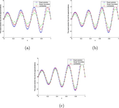
Figure 2. The exact solution and approximate solution of two regularization methods of Example 7.1 with $\alpha =0.9$ for $ϵ=0.001,0.0005,0.0001$. (a) $\alpha =0.9,ϵ=0.001$ (b) $\alpha =0.9,ϵ=0.0005$ (c) $\alpha =0.9,ϵ=0.0001$. (a) $ϵ=0.001$. (b) $ϵ=0.0005$ and (c) $ϵ=0.0001$.

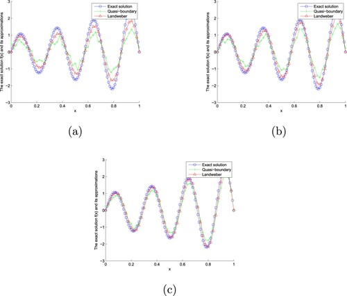
Table 3. Absolute error of two regularization methods of Example 7.1 for different α with $ϵ=0.001,0.0005,0.0001$.

α		0.2	0.4	0.6	0.8
$ϵ=0.001$	Modified quasi-boundary	0.1270	0.1263	0.1242	0.1215
	Landweber	0.0883	0.0833	0.0827	0.0807
$ϵ=0.0005$	Modified quasi-boundary	0.0837	0.0805	0.0786	0.0691
	Landweber	0.0697	0.0621	0.0534	0.0501
$ϵ=0.0001$	Modified quasi-boundary	0.0525	0.0513	0.0506	0.0498
	Landweber	0.0398	0.0371	0.0369	0.0297

Table 4. The CPU time of two regularization methods of Example 7.1 for different α with $ϵ=0.001,0.0005,0.0001$.

α		0.2	0.4	0.6	0.8
$ϵ=0.001$	Modified quasi-boundary	1.4344 s	1.4353 s	1.4425 s	1.4497 s
	Landweber	2.0065 s	2.1973 s	2.3469 s	2.5532 s
$ϵ=0.0005$	Modified quasi-boundary	1.4353 s	1.5084 s	1.5144 s	1.6435 s
	Landweber	3.0850 s	3.0648 s	3.1415 s	3.2095 s
$ϵ=0.0001$	Modified quasi-boundary	1.4518 s	1.4573 s	1.4671 s	1.4727 s
	Landweber	8.6979 s	9.1074 s	9.1760 s	11.9389 s

For the two regularization methods, in Figures 1 and 2, we find that the smaller the erroe level ε, the better the fitting effect. Moreover, the fitting effect of Landweber iterative regularization method is better than that of a modified quasi-boundary regularization method. From Table 3, we find that the smaller α and ε, the smaller the absolute error. Moreover, the error of Landweber iterative regularization method is smaller than that of a modified quasi-boundary regularization method. From Table 4, we find that when α is larger and ε is smaller, the CPU time is longer. In addition, the CPU time of the modified quasi-boundary regularization method is shorter than that of Landweber iterative regularization method.

Figure 3 shows the exact solution and its approximation solution under a modified quasi-boundary regularization method and Landweber iterative regularization method for $\alpha =0.2$ at different error level $ϵ=0.001,ϵ=0.0005,ϵ=0.0001$ with Example 7.2. Figure 4 shows the exact solution and its approximation solution under a modified quasi-boundary regularization method and Landweber iterative regularization method for $\alpha =0.9$ at different error level $ϵ=0.001,ϵ=0.0005,ϵ=0.0001$ with Example 7.2. Table 5 shows the comparison of absolute error of two regularization methods of Example 7.2 for different α with $ϵ=0.001,0.0005,0.0001$. Table 6 shows the comparison of two regularization methods of the CPU time of Example 7.2 for different α with $ϵ=0.001,0.0005,0.0001$.

Figure 3. The exact solution and approximate solution of two regularization methods of Example 7.2 with $\alpha =0.2$ for $ϵ=0.001,0.0005,0.0001$. (a).$\alpha =0.2,ϵ=0.001$ (b).$\alpha =0.2,ϵ=0.0005$ (c).$\alpha =0.2,ϵ=0.0001$. (a) $ϵ=0.001$. (b) $ϵ=0.0005$ and (c) $ϵ=0.0001$.

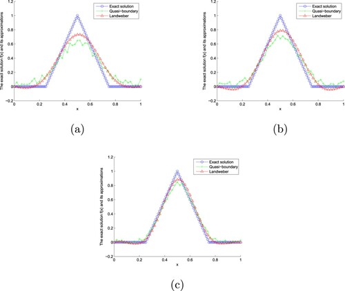
Figure 4. The exact solution and approximate solution of two regularization methods of Example 7.2 with $\alpha =0.9$ for $ϵ=0.001,0.0005,0.0001$. (a).$\alpha =0.9,ϵ=0.001$ (b).$\alpha =0.9,ϵ=0.0005$ (c).$\alpha =0.9,ϵ=0.0001$. (a) $ϵ=0.001$. (b) $ϵ=0.0005$ and (c) $ϵ=0.0001$.

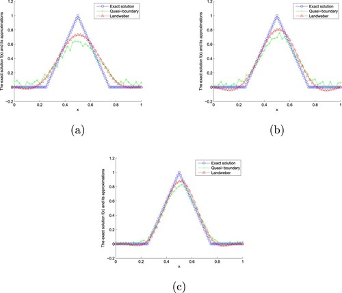
Table 5. Absolute error of two regularization methods of Example 7.2 for different α with $ϵ=0.001,0.0005,0.0001$.

α		0.2	0.4	0.6	0.8
$ϵ=0.001$	Modified quasi-boundary	1.3729 s	1.4792 s	1.4842 s	1.6794 s
	Landweber	3.9500 s	4.0414 s	4.2355 s	4.5106 s
$ϵ=0.0005$	Modified quasi-boundary	1.3997 s	1.4092 s	1.4627 s	1.5114 s
	Landweber	7.5961 s	7.8126 s	8.6522 s	9.4700 s
$ϵ=0.0001$	Modified quasi-boundary	1.4038 s	1.4465 s	1.4480 s	1.6885 s
	Landweber	53.1272 s	55.7849 s	64.6219 s	102.1137 s

Table 6. The CPU time of two regularization methods of Example 7.2 for different α with $ϵ=0.001,0.0005,0.0001$.

α		0.2	0.4	0.6	0.8
$ϵ=0.001$	Modified quasi-boundary	1.4344 s	1.4353 s	1.4425 s	1.4497 s
	Landweber	2.0065 s	2.1973 s	2.3469 s	2.5532 s
$ϵ=0.0005$	Modified quasi-boundary	1.4353 s	1.5084 s	1.5144 s	1.6435 s
	Landweber	3.0850 s	3.0648 s	3.1415 s	3.2095 s
$ϵ=0.0001$	Modified quasi-boundary	1.4518 s	1.4573 s	1.4671 s	1.4727 s
	Landweber	8.6979 s	9.1074 s	9.1760 s	11.9389 s

From Figures 3 and 4, we can find that the smaller ε is, the better the fitting effect is. In addition, compared with the modified quasi-boundary regularization method, the Landweber iterative regularization method is more effective. From Table 5, we find that the smaller α and ε are, the smaller the absolute error is. In addition, compared with the modified quasi-boundary regularization method, the error of Landweber iterative regularization method is smaller. From Table 6, we find that the larger α is, the smaller ε is, the longer the CPU time is. Moreover, the CPU time of the modified quasi-boundary regularization method is shorter than that of Landweber iterative regularization method.

Figure 5 shows the exact solution and its approximation solution under a modified quasi-boundary regularization method and Landweber iterative regularization method for $\alpha =0.2$ at different error level $ϵ=0.001,ϵ=0.0005,ϵ=0.0001$ with Example 7.3. Figure 6 shows the exact solution and its approximation solution under a modified quasi-boundary regularization method and Landweber iterative regularization method for $\alpha =0.9$ at different error level $ϵ=0.001,ϵ=0.0005,ϵ=0.0001$ with Example 7.3. Table 7 shows the comparison of absolute error of two regularization methods of Example 7.3 for different α with $ϵ=0.001,0.0005,0.0001$. Table 8 shows the comparison of two regularization methods of the CPU time of Example 7.3 for different α with $ϵ=0.001,0.0005,0.0001$.

Figure 5. The exact solution and approximate solution of two regularization methods of Example 7.3 with $\alpha =0.2$ for $ϵ=0.001,0.0005,0.0001$. (a).$\alpha =0.2,ϵ=0.001$ (b).$\alpha =0.2,ϵ=0.0005$ (c).$\alpha =0.2,ϵ=0.0001$. (a) $ϵ=0.001$. (b) $ϵ=0.0005$ and (c) $ϵ=0.0001$.

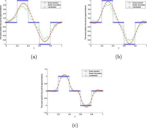
Figure 6. The exact solution and approximate solution of two regularization methods of Example 7.3 with $\alpha =0.9$ for $ϵ=0.001,0.0005,0.0001$. (a).$\alpha =0.9,ϵ=0.001$ (b).$\alpha =0.9,ϵ=0.0005$ (c).$\alpha =0.9,ϵ=0.0001$. (a) $ϵ=0.001$. (b) $ϵ=0.0005$ and (c) $ϵ=0.0001$.

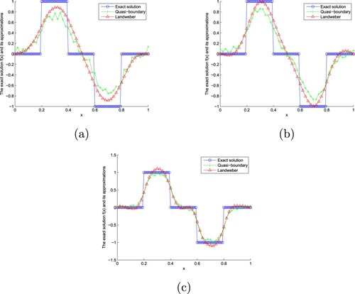
Table 7. Absolute error of two regularization methods of Example 7.3 for different α with $ϵ=0.001,0.0005,0.0001$.

α		0.2	0.4	0.6	0.8
$ϵ=0.001$	Modified quasi-boundary	0.6380	0.6176	0.5940	0.5684
	Landweber	0.3230	0.2987	0.2825	0.2471
$ϵ=0.0005$	Modified quasi-boundary	0.4678	0.4123	0.3875	0.3125
	Landweber	0.2910	0.2654	0.2034	0.1607
$ϵ=0.0001$	Modified quasi-boundary	0.3108	0.3081	0.2405	0.1897
	Landweber	0.2315	0.2017	0.1344	0.0764

Table 8. The CPU time of two regularization methods of Example 7.3 for different α with $ϵ=0.001,0.0005,0.0001$.

α		0.2	0.4	0.6	0.8
$ϵ=0.001$	Modified quasi-boundary	1.4292 s	1.4362 s	1.5370 s	1.5929 s
	Landweber	35.8379 s	42.8959 s	44.9801 s	54.7865 s
$ϵ=0.0005$	Modified quasi-boundary	1.3819 s	1.4017 s	1.4209 s	1.4765 s
	Landweber	47.6532 s	55.5486 s	59.7509 s	73.4390 s
$ϵ=0.0001$	Modified quasi-boundary	1.2366 s	1.4223 s	1.4257 s	1.6837 s
	Landweber	110.3082 s	138.9651 s	139.5039 s	162.1432 s

From Figures 5 and 6, we find that the smaller ε is, the better the fitting effect is. In addition, compared with the modified quasi-boundary regularization method, the Landweber iterative regularization method has better fitting effect. From Table 7, we find that the absolute error decreases with the increase of α and decreases with the decrease of ε. In addition, compared with the modified quasi-boundary regularization method, the error of Landweber iterative regularization method is smaller. From Table 8, we find that the larger α is, the smaller ε is, the longer the CPU time is. In addition, the CPU time of the modified quasi-boundary regularization method is shorter than that of Landweber iterative regularization method.

According to the above three examples of different properties, it can be proved that the absolute error obtained by Landweber iterative regularization method is smaller than that of a modified quasi-boundary regularization method for given α and ε. Moreover, through Figures 1–6, we find that the fitting effect of Landweber iterative regularization method is better than that of a modified quasi-boundary regularization method. Therefore, the Landweber iterative regularization method is more effective than the modified quasi-boundary regularization method. However, in terms of the CPU time, a modified quasi-boundary regularization method is shorter than Landweber iterative regularization method.

8. Conclusion

In this paper, the problem of unknown source identification for space-time fractional diffusion equation is studied. In this equation, the time fractional derivative is a new fractional derivative Caputo-Fabrizio fractional derivative. We prove that this problem is an ill-posed problem. Based on a priori assumption, the optimal error bound analysis of the problem under the source condition is obtained. In addition, we solve the inverse problem (1(1) $\left\{\begin{array}{ll}{}_{CF}{D}_{0,t}^{\alpha }u(x,t)+(-L{)}^{s}u(x,t)=f(x\left)q\right(t),& \mathrm{i}\mathrm{n}\mathrm{\Omega }\times (0,T),\\ u(x,t)=0,& \mathrm{o}\mathrm{n}\mathrm{\partial }\mathrm{\Omega }\times (0,T),\\ u(x,0)=\phi \left(x\right),& \mathrm{i}\mathrm{n}\left\{0\right\}\times \mathrm{\Omega },\\ u(x,T)=g\left(x\right),& x\in \mathrm{\Omega },\end{array}\right.$(1) ) by two different regularization methods. The convergence error estimates of the two regularization methods are obtained under a priori and a posteriori regularization parameter selection rules. Compared with the modified quasi-boundary regularization method, we prove that the convergence error estimates obtained by Landweber iterative regularization method are order optimal. Finally, numerical examples of several different properties are given to demonstrate the advantages and disadvantages, stability and effectiveness of the two regularization methods, and the advantages of the two regularization methods in dealing with the inverse problem.

Disclosure statement

No potential conflict of interest was reported by the authors.

Additional information

Funding

The project is supported by the National Natural Science Foundation of China [grant number 11961044], the Doctor Fund of Lan Zhou University of Technology.

References

- Caputo M, Fabrizio M. A new definition of fractional derivative without singular kernel. Progr Fract Differ Appl. 2015;1(2):73–85.
- Losada J, Nieto JJ. Properties of a new fractional derivative without singular kernel. Progr Fract Differ Appl. 2015;1(2):87–92.
- Tuan NH, Zhou Y. Well-posedness of an initial value problem for fractional diffusion equation with Caputo-Fabrizio derivative. Chaos Soliton Fract. 2020;138:109966.
- Zheng XC, Wang H, Fu HF. Well-posedness of fractional differential equations with variable-order Caputo-Fabrizio derivative. Chaos Soliton Fract. 2020;138:109966.
- Al-Salti N, Karimov E, Kerbal S. Boundary-value problems for fractional heat equation involving Caputo-Fabrizio derivative. New Trends Math Sci. 2016;4(4):79–89.
- Baleanu D, Jajarmi A, Mohammadi H, et al. A new study on the mathematical modelling of human liver with Caputo-Fabrizio fractional derivative. Chaos Soliton Fract. 2020;134:109705.
- Al-khedhairi A. Dynamical analysis and chaos synchronization of a fractional-order novel financial model based on Caputo-Fabrizio derivative. Eur Phys J Plus. 2019;134(10):532.
- Al-Salti N, Karimov E, Sadarangani K. On a differential equation with Caputo-Fabrizio fractional derivative of order 1<β≤2 and application to mass-spring-damper system. Progr Fract Differ Appl. 2016;2(4):257–263.
- Shi JK, Chen MH. A second-order accurate scheme for two-dimensional space fractional diffusion equations with time Caputo-Fabrizio fractional derivative. Appl Numer Math. 2020;151:246–262.
- Liu ZG, Cheng AJ, Li XL. A second order Crank-Nicolson scheme for fractional Cattaneo equation based on new fractional derivative. Appl Math Comput. 2017;311:361–374.
- Wang JG, Wei T, Zhou YB. Tikhonov regularization method for a backward problem for the time-fractional diffusion equation. Appl Math Model. 2013;37(18–19):8518–8532.
- Yang F, Zhang P, Li XX, et al. Tikhonov regularization method for identifying the space-dependent source for time-fractional diffusion equation on a columnar symmetric domain. Adv Differ Equ. 2020;2020:128.
- Yang F, Fu CL, Li XX. A modified tikhonov regularization method for the cauchy problem of Laplace equation. Acta Math Sci. 2015;35(6):1339–1348.
- Xiong XT, Xue X. A fractional Tikhonov regularization method for identifying a space-dependent source in the time-fractional diffusion equation. Appl Math Comput. 2019;349:292–303.
- Yang F, Pu Q, Li XX. The fractional Tikhonov regularization methods for identifying the initial value problem for a time-fractional diffusion equation. J Comput Appl Math. 2020;380:112998.
- Wang JG, Wei T, Zhou Y. Optimal error bound and simplified Tikhonov regularization method for a backward problem for the time-fractional diffusion equation. J Comput Appl Math. 2015;279(18–19):277–292.
- Feng XL, Eldén L. Solving a Cauchy problem for a 3D elliptic PDE with variable coefficients by a quasi-boundary-value method. Inverse Probl. 2014;30(1):015005.
- Yang F, Wang N, Li XX, et al. A quasi-boundary regularization method for identifying the initial value of time-fractional diffusion equation on spherically symmetric domain. Inverse Ill-posed Probl. 2019;27(5):609–621.
- Yang F, Sun YR, Li XX, et al. The quasi-boundary regularization value method for identifying the initial value of heat equation on a columnar symmetric domain. Numer Algor. 2019;82(2):623–639.
- Yang F, Zhang P, Li XX. The truncation method for the Cauchy problem of the inhomogeneous Helmholtz equation. Appl Anal. 2019;98(5):991–1004.
- Yang F, Pu Q, Li XX, et al. The truncation regularization method for identifying the initial value on non-homogeneous time-fractional diffusion-wave equations. Mathematics. 2019;7:1007.
- Wei T, Wang JG. A modified quasi-boundary value method for an inverse source problem of the time-fractional diffusion equation. Appl Numer Math. 2014;78:95–111.
- Yang F, Fu CL, Li XX. A mollification regularization method for unknown source in time-fractional diffusion equation. Int J Comput Math. 2014;91(7):1516–1534.
- Zhang HW, Qin HH, Wei T. A quasi-reversibility regularization method for the Cauchy problem of the Helmholtz equation. Int J Comput Math. 2011;88(4):839–850.
- Yang F, Fu CL. The quasi-reversibility regularization method for identifying the unknown source for time fractional diffusion equation. Appl Math Model. 2015;39(5–6):1500–1512.
- Yang F, Ren YP, Li XX. Landweber iteration regularization method for identifying unknown source on a columnar symmetric domain. Inverse Probl Sci Eng. 2018;26(8):1109–1129.
- Yang F, Liu X, Li XX. Landweber iteration regularization method for identifying unknown source of the modified Helmholtz equation. Bound Value Probl. 2017;2017(1):1–16.
- Yang F, Zhang Y, Li XX. Landweber iteration regularization method for identifying the initial value problem of the time-space fractional diffusion-wave equation. Numer Algor. 2020;83:1509–1530.
- Xiong XT, Fu CL, Li HF. Fourier regularization method of a sideways heat equation for determining surface heat flux. J Math Anal Appl. 2006;317(1):331–348.
- Li XX, Lei JL, Yang F. An a posteriori fourier regularization method for identifying the unknown source of the space-fractional diffusion equation. J Inequal Appl. 2014;2014(1):1–13.
- Yang F, Fu CL, Li XX, et al. The Fourier regularization method for identifying the unknown source for the modified Helmholtz equation. Acta Math Sci. 2014;34(4):1040–1047.
- Yang F, Fan P, Li XX, et al. Fourier truncation regularization method for a time-fractional backward diffusion problem with a nonlinear source. Mathematics. 2019;7(9):865.
- Liu SS, Feng LX. A posteriori regularization parameter choice rule for a modified kernel method for a time-fractional inverse diffusion problem. J Comput Appl Math. 2019;353:355–366.
- Liu SS, Feng LX. Optimal error bound and modified kernel method for a space-fractional backward diffusion problem. Adv Differ Equ. 2018;2018:268.
- Liu SS, Feng LX. A modified kernel method for a time-fractional inverse diffusion problem. Adv Differ Equ. 2015;2015:342.
- Yang F, Fu JL, Li XX. A potential-free field inverse Schrödinger problem: optimal error bound analysis and regularization method. Inverse Probl Sci Eng. 2020;28(9):1209–1252.
- Zhang ZQ, Ma YJ. A modified kernel method for numerical analytic continuation. Inverse Probl Sci Eng. 2013;21(5):840–853.
- Tautenhahn U. Optimality for ill-posed problems under general source conditions. Numer Funct Anal Optim. 1998;19(3–4):377–398.
- Ivanchov MI. The inverse problem of determining the heat source power for a parabolic equation under arbitrary boundary conditions. J Math Sci. 1998;88(3):432–436.
- Schr o¨er T, Tautenhahn U. On the optimal regularization methods for solving linear ill-posed problems. Z Anal Anwend. 1994;13(4):697–710.
- Tautenhahn U. Optimal stable approximations for the sideways heat equation. J Inverse Ill-Posed Probl. 1997;5(3):287–307.
- Vainikko G. On the optimality of methods for ill-posed problems. Z Anal Anwend. 1987;6(4):351–362.
- Hohage T. Regularization of exponentially ill-posed problems. Numer Funct Anal Optim. 2000;21(3–4):439–464.
- Engl HW, Hanke M, Neubauer A. Regularization of inverse problem. Dordrecht: Kluwer Academic Publishers; 1996.
- Tautenhahn U, Gorenflo R. On optimal regularization methods for fractional differentiation. J Anal Appl. 1999;18(2):449–467.
- Tautenhahn U. Optimal stable solution of Cauchy problems for elliptic equations. Z Anal Anwend. 1996;15:961–984.
- Hofmann B, Tautenhahn U, H a¨mrik U. Conditional stability estimates for ill-posed PDE problem by using interpolation. Preprint 2011–16, 2011. Available from: http://nbn-resolving.de/urn:nbn:de:bsz:ch1-qucosa-72654.
- Atangana A, Alqahtani RT. Numerical approximation of the space-time Caputo-Fabrizio fractional derivative and application to groundwater pollution equation. Adv Differ Equ. 2016;2016(1):156.