An inverse source identification by nonlinear optimization in a two-dimensional hyperbolic problem

Abstract

This study deals with the identification of source function from final time state observation in a two-dimensional hyperbolic problem. The solution to the direct problem is obtained by the weak solution approach and finite element method. In the part of the inverse problem, the trust-region method and Levenberg–Marquardt method, which are nonlinear least-squares optimization methods, are used for the identification of source function. The findings are presented with numerical examples.

KEYWORDS:

• Inverse problems
• hyperbolic equations
• finite elements method
• optimization

Mathematical Subject classifications:

• 34M50
• 35L50
• 65M60
• 65K10

1. Introduction

In abstract and applied mathematics, the hyperbolic problems related to wave equations have attracted the attention of many scientists. The desire to get some knowledge about the internal dynamics of the wave from its traceable behaviour has been the reason for this interest. In hyperbolic equations, solutions of the corresponding direct problems may have discontinuities, singular components of complicated structure. As it is known, the more stable an operator is, the harder it is to work with its inverse. In this respect, inverse problems for hyperbolic equations have always been popular.

Considering the spatial variables in the region $\text{x}\in \mathrm{\Omega }\subset {\mathbb{R}}^2$ and time variable in the interval $t\in (0,T]$, let us write the hyperbolic equation on the domain ${\text{Q}}_T:=(\text{x},t)\in \mathrm{\Omega }\times (0,T]$ in the form (1.1) $\begin{array}{rl}& \frac{{\mathrm{\partial }}^{2}u}{\mathrm{\partial }{t}^2}-\mathrm{\nabla }\cdot (c(\text{x})\mathrm{\nabla }u)+a(\text{x},t)u=\sigma (t)f(\text{x}),(\text{x},t)\in {\text{Q}}_T\end{array}$(1.1) (1.2) $\begin{array}{rl}& u(\text{x},0)=u_0(\text{x}),u_t(\text{x},0)=v_0(\text{x}),\text{x}\in \mathrm{\Omega }\end{array}$(1.2) (1.3) $\begin{array}{rl}& u(\text{x},t)=g(t),\text{x}\in \mathrm{\partial }\mathrm{\Omega },t\in (0,T]\end{array}$(1.3) where (1.4) $\begin{array}{rl}& c(\text{x})\in L_{\mathrm{\infty }}(\mathrm{\Omega })\text{and}c(\text{x})>0,a(\text{x},t)\in L_{\mathrm{\infty }}({\text{Q}}_T),\sigma (t)\in L_2(0,T],f(\text{x})\in L_2(\mathrm{\Omega })\\ & u_0(\text{x})\in H^1(\mathrm{\Omega }),v(\text{x})\in L_2(\mathrm{\Omega }),g(t)\in L_2(0,T].\end{array}$(1.4) In vibration modelling, the external forces with the form of separation of variables $\sigma (t)f(\text{x})$ have special meanings. For example, the selection of $\sigma (t)=\cos wt$ describes a harmonic spatial force. Generally, the problem (1.1)–(1.3) is admitted as a model for flexible waves corresponding to a point slipping source. This kind of point source can be connected with models in ground-penetrating radar, reflection seismology, oil and gas exploration and many other physical systems [1].

For a given source $\sigma (t)f(\text{x})$, obtaining the solution $u(\text{x},t)$ of the initial boundary value problem (1.1)–(1.3) is defined as the direct problem. We can conclude from [2] that under the conditions (1.4), the problem (1.1)–(1.3) has a weak solution $u\in C([0,T],H^1(\mathrm{\Omega }))$ with the weak derivatives $u_t\in C([0,T],L_2(\mathrm{\Omega }))$ and $u_{tt}\in C([0,T],H^{-1}(\mathrm{\Omega }))$. Also, this solution satisfies the following estimate: (1.5) $\begin{array}{rl}& \Vert u{\Vert }_{L_{\mathrm{\infty }}(0,T;H^1(\mathrm{\Omega }))}+\Vert u_t{\Vert }_{L_{\mathrm{\infty }}(0,T;L_2(\mathrm{\Omega }))}\\ & \le c({\Vert \sigma \Vert }_{L_2(0,T]}{\Vert f\Vert }_{L_2(\mathrm{\Omega })}+{\Vert u_0\Vert }_{H^1(\mathrm{\Omega })}+{\Vert v\Vert }_{L_2(\mathrm{\Omega })}+\Vert g\Vert {}_{L_2(0,T]})\end{array}$(1.5) Besides, the identification of any unknown data from a given observation related to the solution is defined as the inverse problem.

In this study, we consider the following inverse problem: (1.6) $\text{find the source function}f(\text{x})\text{from}\text{final time state observation}w(\text{x}):=u(\text{x},T;f(\text{x}))$(1.6) where $u(\text{x},T;f(\text{x}))$ represents the solution of the direct problem for a given source $f(\text{x})\in L_2(\mathrm{\Omega })$.

In the last decades, inverse source problems with the final time observation for hyperbolic problems have attracted great attention due to both their significance in engineering applications and significance in the theory of inverse problems [3–10].

The solution of the (1.6) inverse problem is achieved by minimizing the following least-squares functional (1.7) $F(f(\text{x}))=\Vert u(\text{x},T;f(\text{x}))-w(\text{x}){\Vert }^2$(1.7) On the other hand, these types of inverse problems are ill-posed according to Hadamard requirements which are existence, uniqueness and stability of the solution. There are many studies to overcome the ill-posedness by regularization techniques [4,11–14]

The layout of this article is as follows. In Section 2, we have applied the finite element method for weak solution to direct problem. In Section 3, we have implemented a trust-region algorithm and Levenberg–Marquardt method, which are interrelated methods, except for one point, for the identification problem. In the last section, we have tested the proposed methods on two numerical examples.

2. Weak formulation and finite element method for direct problem

Multiplying the equality of (1.1) by a test function $v$, which is zero on the boundary and integrating over the domain, we get the following integral equality for $t\in (0,T]$: ${\int }_{\mathrm{\Omega }}\ddot{u}v\text{dx}-{\int }_{\mathrm{\Omega }}\mathrm{\nabla }\cdot (c\mathrm{\nabla }u)v\text{dx}+{\int }_{\mathrm{\Omega }}auv\text{dx}={\int }_{\mathrm{\Omega }}\sigma (t)f(\text{x})v\text{dx}$and by Green’s formula, we have (2.1) ${\int }_{\mathrm{\Omega }}\ddot{u}v\text{dx}+{\int }_{\mathrm{\Omega }}(c\mathrm{\nabla }u)\cdot \mathrm{\nabla }v\text{dx}-{\int }_{\mathrm{\partial }\mathrm{\Omega }}(c\mathrm{\nabla }u)\cdot \text{n}v\text{ds}+{\int }_{\mathrm{\Omega }}auv\text{dx}={\int }_{\mathrm{\Omega }}\sigma (t)f(\text{x})v\text{dx}$(2.1) By the spaces $H_g^1=\{v:v_{L_2(\mathrm{\Omega })}+\mathrm{\nabla }{v}_{L_2(\mathrm{\Omega })}<\mathrm{\infty },{v|}_{\mathrm{\partial }\mathrm{\Omega }}=g\}$ and $H_0^1=\{v:v_{L_2(\mathrm{\Omega })}+\mathrm{\nabla }{v}_{L_2(\mathrm{\Omega })}<\mathrm{\infty },{v|}_{\mathrm{\partial }\mathrm{\Omega }}=0\}$, the variational formulation of the considered problem is:

find $u\in H_g^1$ such that for every fixed $t\in (0,T]$ and (2.2) ${\int }_{\mathrm{\Omega }}\ddot{u}v\text{dx}+{\int }_{\mathrm{\Omega }}(c\mathrm{\nabla }u)\cdot \mathrm{\nabla }v\text{dx}+{\int }_{\mathrm{\Omega }}auv\text{dx}={\int }_{\mathrm{\Omega }}\sigma (t)f(\text{x})v\text{dx},\mathrm{\forall }v\in H_0^1.$(2.2) Let us apply the finite element method to the direct problem. The domain $\mathrm{\Omega }$ is approximated by the union of $N_T$ elements $\mathrm{\Omega }\approx {\tau }^h\equiv \underset{i=1}{\overset{N_T}{\cup }}{\tau }_i$where ${\tau }_i$ is the $i$th element. The union of the elements is called ${\tau }^h$, and it is the finite element mesh for the domain $\mathrm{\Omega }$. The number $h$ indicates the size of the elements.

We seek the approximate solution in the form (2.3) $u^h(x,y,t)=\sum _{j=1}^{N_p}{U}_j(t){\varphi }_j(x,y)$(2.3) where $N_p$ is the number of the nodes. The basis function ${\varphi }_j(x,y)$ is the second-order Lagrangian shape functions ${\varphi }_j(x,y)=a_1+a_{2}x+a_{3}y+a_4{x}^2+a_{5}xy+a_6{y}^2.$The six coefficients $a_j$ of this polynomial are determined by requiring ${\varphi }_j(x_k,y_k)={\delta }_{jk},j,k=1,2,\dots ,N_p.$With these six parameters, we consider constructing a quadratic Lagrange polynomial by placing nodes at the vertices and mid-sides of a triangular element [15].

Now, considering the approximate solution $u^h$ in (2.2) ${\int }_{\mathrm{\Omega }}{\ddot{u}}_{h}v\text{dx}+{\int }_{\mathrm{\Omega }}(c\mathrm{\nabla }{u}^h)\cdot \mathrm{\nabla }v\text{dx}+{\int }_{\mathrm{\Omega }}a{u}^{h}v\text{dx}={\int }_{\mathrm{\Omega }}\sigma (t)f(\text{x})v\text{dx}$We get $\begin{array}{r}\sum _{j=1}^{N_p}{\ddot{u}}_j(t){\int }_{\mathrm{\Omega }}{\varphi }_{j}v\text{dx}+\sum _{j=1}^{N_p}{U}_j(t){\int }_{\mathrm{\Omega }}(c\mathrm{\nabla }{\varphi }_j)\cdot \mathrm{\nabla }v\text{dx}+\sum _{j=1}^{N_p}{U}_j(t){\int }_{\mathrm{\Omega }}a{\varphi }_{j}v\text{dx}={\int }_{\mathrm{\Omega }}\sigma (t)f(\text{x})v\text{dx}\end{array}$Choosing $v$ to be each of the basis functions ${\varphi }_i,i=1,\dots ,N_p$, we write $\begin{array}{rl}& \sum _{j=1}^{N_p}{\ddot{u}}_j(t){\int }_{\mathrm{\Omega }}{\varphi }_j{\varphi }_i\text{dx}+\sum _{j=1}^{N_p}{U}_j(t){\int }_{\mathrm{\Omega }}(c\mathrm{\nabla }{\varphi }_j)\cdot \mathrm{\nabla }{\varphi }_i\text{dx}+\sum _{j=1}^{N_p}{U}_j(t){\int }_{\mathrm{\Omega }}a{\varphi }_j{\varphi }_i\text{dx}\\ & ={\int }_{\mathrm{\Omega }}\sigma (t)f(\text{x}){\varphi }_i\text{dx},i=1,\dots ,N_p.\end{array}$So, we have $N_p$ unknowns and $N_p$ equations above, which will give a unique solution $U_1,U_2,\dots ,U_{N_p}$.

For solution vector $\text{U}=[U_1,U_2,\dots ,U_{N_p}{]}^{\text{T}}$, we can write the following time-dependent matrix equations: (2.4) $\text{M}\frac{{\text{d}}^2\text{U}}{\text{d}{t}^2}+\text{KU}+\text{A}(t)\text{U}=\text{F}(t)$(2.4) where $\text{M}=M_{ij}={\int }_{\mathrm{\Omega }}{\varphi }_j{\varphi }_i\text{dx},i=1,\dots ,N_p,j=1,\dots ,N_p,$ $\text{K}=K_{ij}={\int }_{\mathrm{\Omega }}(c\mathrm{\nabla }{\varphi }_j)\cdot \mathrm{\nabla }{\varphi }_i\text{dx},i=1,\dots ,N_p,j=1,\dots ,N_p,$ $\text{A}(t)=A_{i,j}={\int }_{\mathrm{\Omega }}a{\varphi }_j{\varphi }_i\text{dx},i=1,\dots ,N_p,j=1,\dots ,N_p,$

and $\text{F}(t)=F_i={\int }_{\mathrm{\Omega }}\sigma (t)f(\text{x}){\varphi }_i\text{dx},i=1,\dots ,N_p.$The equality of (2.4) is the system of second-order ordinary differential equation and the initial conditions come from (1.2) such as $U_j(0)=u_0(P_j),\frac{\text{d}{U}_j}{\text{d}t}(0)=v_0(P_j),j=1,\dots ,N_p$and by vector form ${\text{u}}_0=U_j(0)\text{and}{\text{v}}_0=\frac{\text{d}{U}_j}{\text{d}t}(0).$Hence, we have the system (2.5) $\begin{array}{rl}& \text{M}\frac{d^2\text{U}}{d{t}^2}+\text{KU}+\text{A}(t)\text{U}=\text{F}(t)\\ & {\text{u}}_0=\text{U}(0),{\text{v}}_0=\frac{\text{dU}}{\text{d}t}(0)\end{array}$(2.5) This system can be solved on the time interval $(0,T]$ by any of the numerical methods like Euler's method, Runge–Kutta method or an adaptive scheme. Although the requirement on $\mathrm{\Delta }t$ is not so stringent by an implicit method when solving the hyperbolic problems, we must not forget stability issues. In applying (2.5) to approximate a solution to the hyperbolic equation, we realize that the approximate solution is growing implausible in amplitude, and then the time step must be decreased.

The approximate solution $u^h$ satisfies the a priori estimate [15] (2.6) $\Vert u(t)-u^h(t)\Vert \le C{h}^2\left(\Vert \ddot{u}(t)\Vert +\underset{0}{\overset{t}{\int }}\Vert \ddot{u}(.,s)\Vert \text{d}s\right)$(2.6)

3. Solution of inverse identification problem

In order to get the unknown source function from the given final time observation by (1.7), we will use the nonlinear least-squares optimization for the problem (3.1) $f^{\ast }=\underset{f}{\text{argmin}}F(f(\text{x}))$(3.1) where $F(f(\text{x}))=\Vert u(\text{x},T;f(\text{x}))-w(\text{x}){\Vert }^2=\Vert \text{r}(f){\Vert }^2=\sum _{j=1}^{N_p}[u^h(P_j,T;f(P_j))-w(P_j){]}^2$and the components of $\text{r}(f)$ are defined as $r_j(f)=u^h(P_j,T;f(P_j))-w(P_j),j=1,2,\dots ,N_p$.

Considering the compatibility conditions, the structure of identified function $f(\text{x})$ is estimated and appropriate parameters $\text{c}=\{c_1,c_2,\dots ,c_m\}$ are included to this function. So, it is assumed that we want to get ${\text{c}}^{\ast }$, which is the minimum of the objective function $F(\text{c}):{\mathbb{R}}^m\stackrel{\text{r}}{\to }{\mathbb{R}}^{N_p}\to \mathbb{R}-.$Namely, the problem (3.1) is reformulated as follows: (3.2) $f^{\ast }:=F^{\ast }({\text{c}}^{\ast })=\underset{\text{c}}{\text{argmin}}\Vert u^h(P_j,T;f(P_j))-w(P_j){\Vert }^2$(3.2) Let us write the Taylor approximation by the degree 2 of $F$ around any $\text{c}$: $F(\text{c}+\mathrm{\Delta }\text{c})\cong L(\mathrm{\Delta }\text{c})=F(\text{c})+(\mathrm{\Delta }\text{c}{)}^{\text{T}}\text{g}+\frac{1}{2}(\mathrm{\Delta }\text{c}{)}^{\text{T}}\text{ B }(\mathrm{\Delta }\text{c})$where $L(\mathrm{\Delta }\text{c})$ is the quadratic approximation of $F(\text{c})$ around $\text{c}$, $\text{g}$ the gradient of $F(\text{c})$ computed at $\text{c}$, $\text{B}$ an approximation of the Hessian matrix $\text{H}$ of $F(\text{c})$ at $\text{c}$ and $\text{H}$ the real hessian matrix of $F(\text{c})$ at $\text{c}$.

Also, we know, from the optimization theory that if ${\text{c}}^{\ast }$ is a local minimizer, then $\text{g}({\text{c}}^{\ast })=0$ (Necessary condition for a local minimizer) and $(\mathrm{\Delta }\text{c}{)}^{\text{T}}\text{B}({\text{c}}^{\ast })(\mathrm{\Delta }\text{c})>\delta \Vert \mathrm{\Delta }\text{c}{\Vert }^2$ (Positive definiteness – Sufficient condition for a local minimizer), with some number $\delta >0$. So, we must always construct the positive definite $\text{B}$ matrix.

In the remaining of the paper, we use the 2-norm, $\Vert c\Vert =\sqrt{c_1^2+\dots +c_m^2}$.

On the other hand, we know, from the vector analysis that the gradient at $\text{c}$ is $\text{g}(\text{c})=\text{J}(\text{c}{)}^{\text{T}}\text{ r}(\text{c})$ where $\text{r}(\text{c})$ is the vector whose components are defined as follows: $r_j(\text{c})=u^h(P_j,T;f(P_j;\text{c}))-w(P_j),j=1,2,\dots ,N_p.$Hessian at $\text{c}$ is $\text{H}(\text{c})=\text{J}(\text{c}{)}^{\text{T}}\text{J}(\text{c})+\sum _{j=1}^{N_p}{r}_j(\text{c}){\text{r}}_j^{{}^{\mathrm{\prime }\mathrm{\prime }}}(\text{c})$ and approximation of Hessian at $\text{c}$ is $\text{B}(\text{c})=\text{J}(\text{c}{)}^{\text{T}}\text{J}(\text{c})$. Here, $\text{J}(\text{c})=[J_{ij}{]}_{N_p\times m}=\frac{\mathrm{\partial }{r}_i}{\mathrm{\partial }{c}_j}(\text{c})$ is the partial derivative (Jacobian) of $r_i$ with respect to $c_j$.

According to the Gauss–Newton method, the computation of the step $\mathrm{\Delta }\text{c}$ involves the solution of the linear system (3.3) $(\text{J}{(\text{c})}^{\text{T}}\text{J}(\text{c}))\mathrm{\Delta }\text{c}=-\text{J}(\text{c}{)}^{\text{T}}\text{r}(\text{c}).$(3.3) One difficulty of using the Gauss–Newton step is that the Jacobi matrix $\text{J}(\text{c})$ may be ill-conditioned, which normally leads to a very big step $\mathrm{\Delta }\text{c}$. And a very long step $\mathrm{\Delta }\text{c}$ usually causes the algorithm to break down, because of either numerical overflows or failure in line searches. So, when the Gauss–Newton method is used for ill-conditioned problems, it is not efficient about convergence relations. The main difficulty is that the step size $\mathrm{\Delta }\text{c}$ is too large and goes in a ‘bad’ direction that gives little reduction in the function.

We can handle this issue via the use of a Lagrange multiplier and thus replace the problem (3.4) $(\text{J}{(\text{c})}^{\text{T}}\text{J}(\text{c})+\lambda I)\mathrm{\Delta }\text{c}=-\text{J}(\text{c}{)}^{\text{T}}\text{r}(\text{c}),$(3.4) where $\lambda >0$ is the Lagrange multiplier for the constraint at the $k$th iteration.

The parameter $\lambda$ affects both the direction and the length of the step $\mathrm{\Delta }\text{c}$. Depending on the size of $\lambda$, the correction $\mathrm{\Delta }\text{c}$ can vary from a Gauss–Newton step for $\lambda =0$ to a very short step approximately in the steepest descent direction for large values of $\lambda$. As we see from these considerations, this parameter acts similar to the step control for the damped Gauss–Newton method, but it also changes the direction of the correction.

There are two effective methods for solving such nonlinear equations: Levenberg–Marquardt method, first given by Levenberg [16] and re-derived by Marquardt [17], and trust-region method [18,19]. They are both Gauss–Newton-based methods and expose quadratic speed of convergence near ${\text{c}}^{\ast }$.

The Levenberg–Marquardt step of (3.4) can be interpreted as solving the normal equations used in the Gauss–Newton method, but ‘shifted’ by a scaled identity matrix, so as to convert the problem from having an ill-conditioned (or positive semi-definite) matrix $\text{J}(\text{c}{)}^{\text{T}}\text{J}(\text{c})$ into a positive definite one. Notice that the positive definiteness implies that the Levenberg–Marquardt direction has always descent and, therefore, the method is well defined. During the process, the size of $\lambda$ is updated by controlling the gain ratio $\rho =\frac{\text{actual decrease}}{\text{predicted decrease}}=\frac{F(\text{c})-F(\text{c}+\mathrm{\Delta }\text{c})}{L(0)-L(\mathrm{\Delta }\text{c})}$A large value of $\rho$ implies that $L(\mathrm{\Delta }\text{c})$ is a good approximation to $F(\text{c}+\mathrm{\Delta }\text{c})$ and we can decrease $\lambda$ so that the next Levenberg–Marquardt step is closer to the Gauss–Newton step. If $\rho$ is small or negative then $L(\mathrm{\Delta }\text{c})$ is a poor approximation and we must increase $\lambda$ to get steepest descent direction and reduce the step length.

The Levenberg–Marquardt method’s algorithm is as follows;

Levenberg–Marquardt method’s algorithm

Table

begin

$k:=0$

found:= $\Vert \text{J}{({\text{c}}^k)}^{\text{T}}\text{r}({\text{c}}^k)\Vert \le {\epsilon }_1$, $\lambda :=\zeta \times \text{max}\{a_{ii}\}$

while (not found) and ($k<k_{\text{max}}$)

$k:=k+1$, Solve (3.4) for $\mathrm{\Delta }{\text{c}}_k$.

if $\Vert \mathrm{\Delta }{\text{c}}^k\Vert \le {\epsilon }_2(\Vert {\text{c}}^k\Vert +{\epsilon }_2)$

found:= true

else

${\text{c}}^{k+1}={\text{c}}^k+\mathrm{\Delta }{\text{c}}^k$

${\rho }_k={\displaystyle \frac{F({\text{c}}^k)-F({\text{c}}^{k+1})}{{\displaystyle \frac{1}{2}}\mathrm{\Delta }{({\text{c}}^k)}^{\text{T}}({\lambda }_k\mathrm{\Delta }({\text{c}}^k)-\text{J}{({\text{c}}^k)}^{\text{T}}\text{r}({\text{c}}^k))}}$

if ${\rho }_k>0$

${\text{c}}^{k+1}={\text{c}}^k$

$\text{found}:=\Vert \text{J}{({\text{c}}^{k+1})}^{\text{T}}\text{r}({\text{c}}^{k+1})\Vert \le {\epsilon }_1$

$\lambda :=\lambda \times \text{max}\left\{{\displaystyle \frac{1}{3}},1-{(2{\rho }_k-1)}^3\right\},\nu :=2$

else

$\lambda :=\lambda \times \nu$, $\nu :=2\times \nu$

End

The choice of $\zeta$ should be a small value, e.g. $\zeta ={10}^{-6}.$ $a_{ii}$ is computed by the diagonal components in $\text{J}({\text{c}}^0{)}^{\text{T}}\text{r}({\text{c}}^0)$. ${\epsilon }_1$, ${\epsilon }_2$ and $k_{\text{max}}$ are chosen by the user. The inequalities $\Vert \text{J}{({\text{c}}^k)}^{\text{T}}\text{r}({\text{c}}^k)\Vert \le {\epsilon }_1$ and $\Vert \mathrm{\Delta }{\text{c}}^k\Vert \le {\epsilon }_2(\Vert {\text{c}}^k\Vert +{\epsilon }_2)$ are appropriate stopping criteria and $k<k_{\text{max}}$ is a safeguard against an infinite loop.

On the other hand, reduction in the step size $\Vert \mathrm{\Delta }c\Vert$ is important. It can be proven that, if we apply a proper limitation on the step size $\Vert \mathrm{\Delta }c\Vert \le \delta$, we sustain global convergence even if $\text{J}(\text{c}{)}^{\text{T}}\text{J}(\text{c})$ is an indefinite matrix. The trust-region algorithm is based on this rule ($\delta$ is called the region radius).

In a trust-region method, it is assumed that the model is sufficiently accurate inside a ball with radius $\delta$(trust-region radius) centred at $\text{c}$ and the step $\mathrm{\Delta }\text{c}$ is to solution to a constrained optimization problem (3.5) $\begin{array}{cc}\text{minimize}& L[\mathrm{\Delta }(\text{c})]=F(\text{c})+{(\mathrm{\Delta }\text{c})}^{\text{T}}\text{g}+\frac{1}{2}{(\mathrm{\Delta }\text{c})}^{\text{T}}\text{ B }(\mathrm{\Delta }\text{c})\\ \text{subject to}& \Vert \mathrm{\Delta }\text{c}\Vert \le \delta \end{array}$(3.5) Indeed, a trust-region algorithm for nonlinear least-squares and Levenberg–Marquardt method are similar, apart from the bound $\delta$ is updated from iteration to iteration directly instead of updating parameter $\lambda$.

Trust-region method’s algorithm is as follows:

Trust-region method’s algorithm

Table

begin

$k:=0$, $\delta ={\delta }_0$

$\text{found: = }\Vert \text{J}{({\text{c}}^k)}^{\text{T}}\text{r}({\text{c}}^k)\Vert \le {\epsilon }_1$,

while (not found) and ($k<k_{\text{max}}$)

$k:=k+1$, Solve (3.4) for $\mathrm{\Delta }{\text{c}}_k$.

if $\Vert \mathrm{\Delta }{\text{c}}^k\Vert \le {\epsilon }_2(\Vert {\text{c}}^k\Vert +{\epsilon }_2)$

found:= true

else

${\text{c}}^{k+1}={\text{c}}^k+\mathrm{\Delta }{\text{c}}^k$

${\rho }_k={\displaystyle \frac{F({\text{c}}^k)-F({\text{c}}^{k+1})}{{\displaystyle \frac{1}{2}}\mathrm{\Delta }{({\text{c}}^k)}^{\text{T}}({\lambda }_k\mathrm{\Delta }({\text{c}}^k)-\text{J}{({\text{c}}^k)}^{\text{T}}\text{r}({\text{c}}^k))}}$

if ${\rho }_k>0$

${\text{c}}^{k+1}={\text{c}}^k$

$\text{found: = }\Vert \text{J}{({\text{c}}^{k+1})}^{\text{T}}\text{r}({\text{c}}^{k+1})\Vert \le {\epsilon }_1$

if ${\rho }_k>0.75$

$\delta :=\text{max}\{\delta ,3\Vert \mathrm{\Delta }{\text{c}}^k\Vert \}$

else if ${\rho }_k<0.25$

$\delta :=\delta /2$ found:= $\delta \le {\epsilon }_2(\Vert {\text{c}}^k\Vert +{\epsilon }_2)$

End

Modifying $\delta$ directly has the advantage of controlling and observing the length of $\mathrm{\Delta }\text{c}$ easily. Hence, nowadays, it is regarded that the trust-region approach is better than the original Levenberg–Marquardt method. A detailed information for the trust-region method can be found in [20,21].

4. Numerical illustrations

Now, we aim to test the explained process by giving on two problems. In solving these problems, we have used the MATLAB-2019 software.

Example 1 Consider the material occupying $\mathrm{\Omega }=\{(x,y):(x,y)\in (1,4)\times (1,5)\mathrm{\setminus }(2,3)\times (3,5)\}$.

On the time interval $t\in (0,1]$, we have the problem (4.1) $\begin{array}{rl}& \frac{{\mathrm{\partial }}^{2}u}{\mathrm{\partial }{t}^2}-\mathrm{\nabla }\cdot (\mathrm{\nabla }u)=\cos tf(\text{x}),(\text{x},t)\in {\text{Q}}_1\end{array}$(4.1) (4.2) $\begin{array}{rl}& u(\text{x},0)=0,u_t(\text{x},0)=0,\text{x}\in \mathrm{\Omega }\end{array}$(4.2) (4.3) $\begin{array}{rl}& u(\text{x},t)=0,\text{x}\in \mathrm{\partial }\mathrm{\Omega },t\in (0,1]\end{array}$(4.3)

and want to identify the $f(\text{x})$ source function from the final time state information (4.4) $w(\text{x})=u(\text{x},1)=\sin \pi x\sin \pi y\left(\cos \sqrt{2}\pi -\cos 1\right).$(4.4) The exact source function is $f(\text{x})=(1-2{\pi }^2)\sin \pi x\sin \pi y$.

Firstly, let us compute the solution of direct problem $f(\text{x})\to u(\text{x},1)$ by the finite element method.

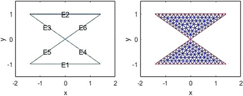
The domain $\mathrm{\Omega }$ is approximated by the union of $N_T$ elements such as $\mathrm{\Omega }\approx {\tau }^h\equiv \underset{i=1}{\overset{N_T}{\cup }}{\tau }_i.$In the following, there are the figures of the domain and a finite element mesh for the problem.

The numbers of elements and nodes are 1033 and 2188, respectively, for the mesh size $h=0.15$.

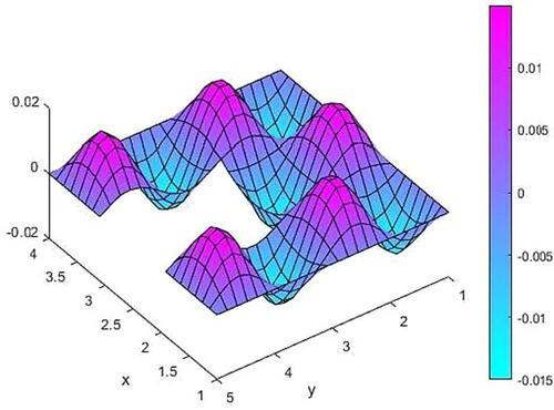
The exact solution $u(\text{x},1)$ and the calculated solution of the finite element method $u^h(\text{x},1)$ by (2.5) are presented in Figures 1–3.

Figure 1. The domain and finite element mesh for $h=0.15$.

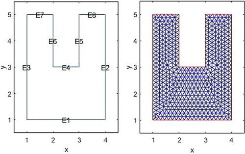
Figure 2. Exact wave function at $T=1$.

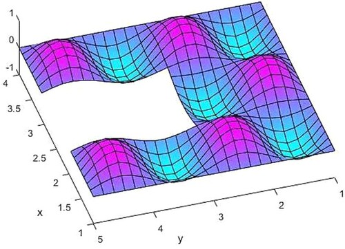
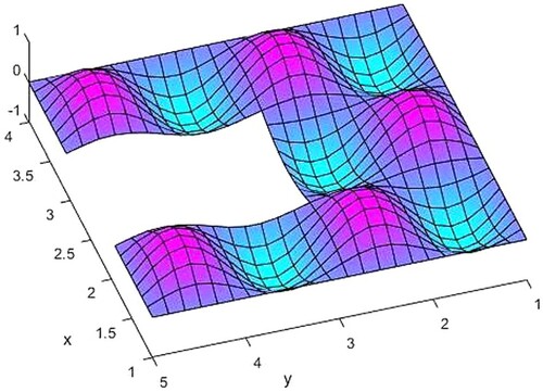
Figure 3. Calculated wave function at $T=1$.

Some error norm values corresponding different $h$ maximum mesh size are given in Table 1. Due to ill-conditioning of some matrices in (2.5), it can be seen by $h=0.15$ and $h=0.1$ in Table 1 that a smaller $h$ value gives a bigger error norm. Hence, we take the $h=0.15$ mesh size for this example. Figure 4 shows the error of the computation for this mesh size.

Figure 4. Error values for $h=0.15$.

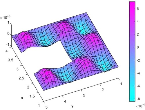
Table 1. Some $h$ and corresponding error norm values.

$\mathit{h}$	$\Vert \mathit{u}(\mathbf{\text{x}},1)-{\mathit{u}}^{\mathit{h}}(\mathbf{\text{x}},1)\Vert$
0.3	0.0775
0.25	0.0360
0.2	0.0127
0.15	0.0107
0.1	0.0532

Secondly, we deal with the solution of the inverse identification problem $w(\text{x})\to f(\text{x})$ by nonlinear least-squares optimization techniques.

From the given final time state function $w(\text{x})=\sin \pi x\sin \pi y\left(\cos \sqrt{2}\pi -\cos 1\right)$, we can estimate that the source function may have the form (4.5) $f(\text{x})=c\sin \pi x\sin \pi y.$(4.5) On the other hand, the exact source function leading to the given final time state function is $f_{\text{exact}}(\text{x})=(1-2{\pi }^2)\sin \pi x\sin \pi y\cong -18.7392\sin \pi x\sin \pi y.$The minimization is carried out by the single-parameter functional (4.6) $F(c)=\underset{c}{\text{argmin}}{u}^{0.15}(P_j,1;f(P_j))-w(P_j{)}^2.$(4.6) If minimization of this functional by the Levenberg–Marquardt method and trust-region method is carried out using MATLAB then the following outcomes are obtained.

For the Levenberg–Marquardt method, we get Table 2.

Table 2. Levenberg–Marquardt method.

Iteration	Function evaluations	Residual	First-order optimality	Lambda	Norm of step
0	3	339.808	18	0.1
1	6	8.75e−04	2.88e−02	0.001	18.6994
2	9	1.85787e−05	2.65e−05	0.001	2.9718e−02
3	12	1.8578e−05	6.57e−08	1e−05	2.7724e−05

Optimization is completed by the Levenberg–Marquardt method since the relative norm of the current step $(3.67\text{e}-09)$ is less than the value of the step tolerance $(1\text{e}-06)$. The found optimal parameter is ${\text{c}}_{\text{Levenberg}-\text{Marquardt}}^{\ast }=-18.72911864359083$. Hence, the identified source function is (4.7) $f_{\text{Levenberg}-\text{Marquardt}}^{\ast }(\text{x})=-18.72911864359083\sin \pi x\sin \pi y$(4.7) The residual norm given by (4.6) for this function is $F^{\ast }=1.857800410424216\text{e}-05$.

For the trust-region method, we get Table 3.

Table 3. Trust-region method.

Iteration	Function evaluations	Residual	First-order optimality	Norm of step
0	3	339.808	18
1	6	73.7256	8.38	10
2	9	4.888e−03	0.0687	8.80035
3	12	1.86689e−05	2.93e−04	7.09e−02
4	15	1.8578e−05	4.08e−07	3.09e−04

Optimization is completed by the trust-region method since the size of the gradient $(4.08\text{e}-07)$, which is the first-order optimality measure, is less than the value of the optimality tolerance $(1\text{e}-06)$. The found optimal parameter is ${\text{c}}_{\text{trust - region}}^{\ast }=-18.72911914110111$. Hence, the identified source function is (4.8) $f_{\text{trust - region}}^{\ast }(\text{x})=-18.72911914110111\sin \pi x\sin \pi y$(4.8) The residual norm given by (4.6) for this function is $F^{\ast }=1.857800460571223\text{e}-05$.

The difference between the optimal parameter values of two methods is $\Vert {\text{c}}_{\text{Levenberg}-\text{Marquardt}}^{\ast }-{\text{c}}_{\text{trust}-\text{region}}^{\ast }\Vert =4.9751\text{e}-07.$As seen the parameters of these methods are too close to each other. If we take the optimal parameter as ${\text{c}}_{}^{\ast }\cong -18.7291$ then we get the following error norm (4.9) $\Vert f_{\text{exact}}(\text{x})-f_{}^{\ast }(\text{x})\Vert =\mathrm{0.2310.}$(4.9) As seen in this example, the Levenberg–Marquardt method was able to calculate the result with the same success using less iteration.

Now, we will examine that the problem needs regularization process or not. To do this, we generate random noisy data $w_{\text{noisy}}(P_j)$. The noisy data are simulated as (4.10) $w_{\text{noisy}}(P_j)=w(P_j)+\rho (P_j)w(P_j)$(4.10) where $\rho (P_j)$ are random variables with the mean zero and standard deviation $\sigma$ given by $\sigma =\gamma$, where $\gamma$ represents the percentage of noise. The random variables $\rho (P_j)=\text{normrnd}(0,\sigma ,\text{length}(P_j))$ is generated by normrnd MATLAB function.

Firstly, we generate random noisy data with the percentage of 10% in the observation function and measure the difference between the source functions caused by this noise.

The optimal parameters accompanying with noisy source function are ${\text{c}}_{\text{trust}-\text{region}}^{\ast (\text{noisy})}-18.701749615205685$ and ${\text{c}}_{\text{Levenberg}-\text{Marquardt}}^{\ast (\text{noisy})}=-18.701748831381636$.

The 10% noise causes the $\frac{\Vert w_{\text{noisy}}(P_j)-w(P_j)\Vert }{\Vert w(P_j)\Vert }=0.1587$ norm between observation functions and $\frac{\Vert f^{\ast }(\text{x};w(P_j))-f^{\ast }(\text{x};w_{\text{noisy}}(P_j))\Vert }{\Vert f^{\ast }(\text{x};w(P_j))\Vert }=0.0018$ norm between source functions.

Secondly, we generate random noisy data with the percentage of 2% in the observation function and measure the difference between the source functions caused by this noise (Figures 5–8).

Figure 5. The difference between the exact and 10% noisy observation function.

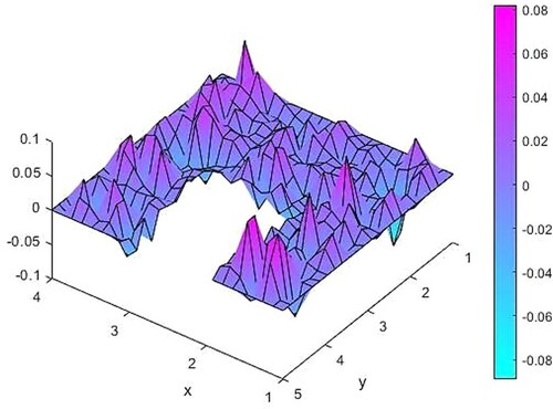
Figure 6. The difference between source functions corresponding to the exact and 10% noisy observation function.

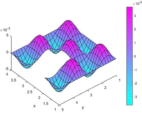
Figure 7. The difference between the exact and 2% noisy observation function.

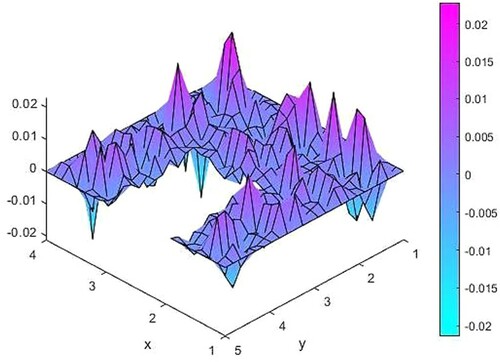
Figure 8. The difference between source functions corresponding to the exact and 2% noisy observation function.

The optimal parameters accompanying with noisy source function are ${\text{c}}_{\text{trust}-\text{region}}^{\ast (\text{noisy})}=-18.712029543267924$ and ${\text{c}}_{\text{Levenberg}-\text{Marquardt}}^{\ast (\text{noisy})}=-18.712029495721413$.

The 2% noise causes the $\frac{\Vert w_{\text{noisy}}(P_j)-w(P_j)\Vert }{\Vert w(P_j)\Vert }=0.0159$ norm between observation functions and $\frac{\Vert f^{\ast }(\text{x};w(P_j))-f^{\ast }(\text{x};w_{\text{noisy}}(P_j))\Vert }{\Vert f^{\ast }(\text{x};w(P_j))\Vert }=0.00091$ norm between source functions.

In Table 4, we present norms of some noisy observations and corresponding source function differences.

Table 4. Some noisy observations and source function differences.

Noise per cent	${\displaystyle \frac{\Vert w-w_{\text{noisy}}\Vert }{\Vert w\Vert }}$	$c_{\text{noisy}}^{\ast }$	${\displaystyle \frac{\Vert f(w)-f^{\ast }(w_{\text{noisy}})\Vert }{\Vert f(w)\Vert }}$	${\displaystyle \frac{\Vert u^{0.15}(c_{\text{noisy}}^{\ast })-w_{\text{noisy}}\Vert }{\Vert u^{0.15}(c_{\text{noisy}}^{\ast })\Vert }}$
20%	0.1587	−18.6944	0.0018	0.1586
10%	0.0779	−18.7017	0.00146	0.0778
2%	0.0159	−18.7120	0.00091	0.0158
1%	0.0079	−18.7208	0.00044	0.0078
0.5%	0.0039	−18.7292	5.34e−06	0.004
0	0	−18.7291	0	0

As seen from Table 4, while noise levels decrease, the corresponding source function differences also decrease. Hence, there is no need for regularization process.

Example 2 Consider the material occupying the domain bounded by the lines $y=\mp \frac{1}{\sqrt{2}}x$ and $y=\mp 1$.

On the time interval $t\in (0,2]$, we have the problem (4.11) $\begin{array}{rl}& \frac{{\mathrm{\partial }}^{2}u}{\mathrm{\partial }{t}^2}-\mathrm{\nabla }\cdot ((x+y)\mathrm{\nabla }u)+2u={\text{e}}^{\frac{t}{2}}f(\text{x}),(\text{x},t)\in {\text{Q}}_2\end{array}$(4.11) (4.12) $\begin{array}{rl}& u(\text{x},0)=x^2-2y^2,u_t(\text{x},0)=\frac{1}{2}(x^2-2y^2),\text{x}\in \mathrm{\Omega }\end{array}$(4.12) (4.13) $\begin{array}{rl}& u(\text{x},t)=\{\begin{array}{cc}0& \text{on }y=\mp \frac{1}{\sqrt{2}}x\\ {\text{e}}^{\frac{t}{2}}(x^2-2)& \text{on }y=\mp 1\end{array},t\in (0,2].\end{array}$(4.13)

and want to identify the $f(\text{x})$ source function from the final time state information (4.14) $w(\text{x})=u(\text{x},2)={\text{e}}^1(x^2-2y^2).$(4.14) The exact source function is $f(\text{x})=0.25x^2+5.5y^2$.

Firstly, let us compute the solution of direct problem $f(\text{x})\to u(\text{x},2)$ by finite element method.

In the following, there are the figures of domain and a finite element mesh for the problem (Figure 9).

Figure 9. The domain and finite element mesh for $h=0.15$.

The numbers of elements and nodes are 292 and 671, respectively, for the mesh size $h=0.15$.

The exact solution $u(\text{x},2)$ and the calculated solution of the finite element method $u^h(\text{x},2)$ by (2.5) are presented in Figures 10–12.

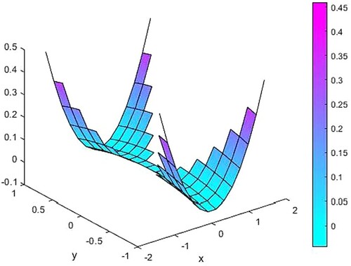
Figure 10. Exact wave function at $T=2$.

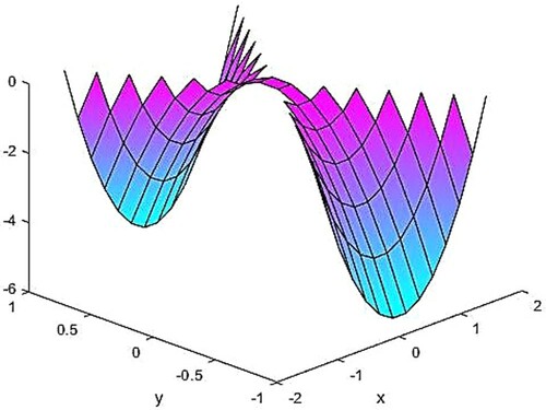
Figure 11. Calculated wave function at $T=2$.

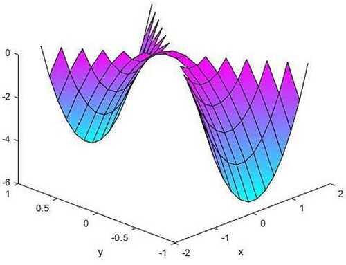
Figure 12. Error values for $h=0.15$_.

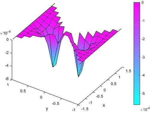
Figure 13. The difference between exact and 10% noisy observation function.

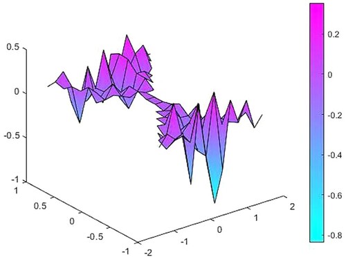
Figure 14. The difference between source functions corresponding to the exact and 10% noisy observation function.

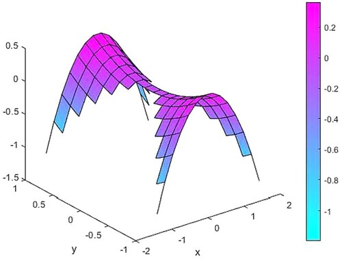
Figure 15. The difference between the exact and 2% noisy observation function.

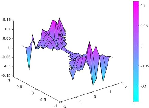
Figure 16. The difference between source functions corresponding to the exact and 2% noisy observation function.

Some error norm values corresponding different $h$ maximum mesh size are given in Table 5. Due to ill-conditioning of some matrices in (2.5), it can be seen by $h=0.15$ and $h=0.1$ in Table 1 that a smaller $h$ value gives a bigger error norm. Hence, we take the $h=0.15$ mesh size for this example. Figure 4 shows the error of the computation for this mesh size .

Table 5. Some $h$ and corresponding error norm values.

$\mathit{h}$	$\Vert \mathit{u}(\mathbf{\text{x}},2)-{\mathit{u}}^{\mathit{h}}(\mathbf{\text{x}},2)\Vert$
0.3	0.0230
0.25	0.0173
0.2	0.0101
0.15	0.0059
0.1	0.0068

Secondly, we deal with the solution of inverse identification problem $w(\text{x})\to f(\text{x})$ by nonlinear least-squares optimization techniques.

From a given final time state function $w(\text{x})=e^1(x^2-2y^2)$, we can estimate that the source function may have the form (4.15) $f(\text{x})=c_1{x}^2+c_2{y}^2.$(4.15) On the other hand, the exact source function leading to a given final time state function is (4.16) $f_{\text{exact}}(\text{x})=0.25x^2+5.5y^2$(4.16) The minimization is carried out by the single-parameter functional (4.17) $F(c_1,c_2)=\underset{(c_1,c_2)}{\text{argmin}}\Vert u^{0.15}(P_j,2;f(P_j))-w(P_j){\Vert }^2$(4.17) If minimization of this functional by the Levenberg–Marquardt method and trust-region method is carried out using MATLAB then the following outcomes are obtained.

For the Levenberg–Marquardt method, we get Table 6.

Table 6. Levenberg–Marquardt method.

Iteration	Function evaluations	Residual	First-order optimality	Lambda	Norm of step
0	5	50.1863	9.02	0.01
1	10	4.87921e−03	0.062	0.001	5.4247
2	15	7.75463e−05	0.00811	0.0001	0.229911
3	20	3.38125e−05	3.54e−06	1e−05	0.0100063
4	25	3.38123e−05	6.6e−07	1e−06	8.71107e−05
5	30	3.38123e−05	2.86e−07	1e−07	1.48894e−05

Optimization is completed by the Levenberg–Marquardt method since the final change in the sum of squares relative to its initial value is less than the value of the function tolerance $(1\text{e}-06)$. The found optimal parameter is ${\text{c}}_{\text{Levenberg}-\text{Marquardt}}^{\ast }=[0.246809936178489,5.500964113399660]$. Hence, the identified source function is (4.18) $f_{\text{Levenberg}-\text{Marquardt}}^{\ast }(\text{x})=0.246809936178489x^2+5.500964113399660y^2$(4.18) The residual norm given by (4.16) for this function is $F^{\ast }=3.381226871464835\text{e}-05$.

For the trust-region method, we get Table 7.

Table 7. Trust-region method.

Iteration	Function evaluations	Residual	First-order optimality	Norm of step
0	5	50.1863	9.02
1	10	7.07137e−05	0.00764	5.501
2	15	3.38123e−05	3.46e−06	0.00654803
3	20	3.38123e−05	1.12e−06	6.86794e−06

Optimization is completed by the trust-region method since the final change in the sum of squares relative to its initial value is less than the value of the function tolerance $(1\text{e}-06)$. The found optimal parameter is ${\text{c}}_{\text{trust - region}}^{\ast }=[0.246811657528541,5.500963848795268]$. Hence, the identified source function is (4.19) $f_{\text{trust - region}}^{\ast }(\text{x})=0.246811657528541x^2+5.500963848795268y^2$(4.19) The residual norm given by (4.6) for this function is $F^{\ast }=3.381227400848656\text{e}-05$.

The difference between the optimal parameter values of two methods is $\Vert {\text{c}}_{\text{Levenberg}-\text{Marquardt}}^{\ast }-{\text{c}}_{\text{trust - region}}^{\ast }\Vert =1.741568\text{e}-06.$As seen, the parameters of these methods are too close to each other. If we take the optimal parameter as ${\text{c}}_{}^{\ast }\cong [0.24681,5.50096]$ then we get the following error norm (4.20) $\Vert f_{\text{exact}}(\text{x})-f_{}^{\ast }(\text{x})\Vert =0.0398$(4.20) As seen in this example, the trust-region method was able to calculate the result with the same success using less iteration.

Now, we generate random noisy data $w_{\text{noisy}}(P_j)$ by (4.10) to decide the regularization process is needed or not (Figures 13–16).

Firstly, we generate random noisy data with the percentage of 10% in the observation function and measure the difference between the source functions caused by this noise.

The optimal parameters accompanying with noisy source function are ${\text{c}}_{\text{trust - region}}^{\ast (\text{noisy})}=[1.034134676584133,5.123458167646760]$ and ${\text{c}}_{\text{Levenberg}-\text{Marquardt}}^{\ast (\text{noisy})}=[1.016975683797493,5.127563889242101]$.

The 10% noise causes the $\frac{\Vert w_{\text{noisy}}(P_j)-w(P_j)\Vert }{\Vert w(P_j)\Vert }=0.0930$ norm between observation functions and $\frac{\Vert f^{\ast }(\text{x};w(P_j))-f^{\ast }(\text{x};w_{\text{noisy}}(P_j))\Vert }{\Vert f^{\ast }(\text{x};w(P_j))\Vert }=0.0986$ norm between source functions (for the trust-region method).

Secondly, we generate random noisy data with the percentage of 2% in the observation function and measure the difference between the source functions caused by this noise.

The optimal parameters accompanying with noisy source function are ${\text{c}}_{\text{trust - region}}^{\ast (\text{noisy})}=[-0.006929996321541,5.548445550509578]$ and ${\text{c}}_{\text{Levenberg}-\text{Marquardt}}^{\ast (\text{noisy})}=[-0.006472533875535,5.548249867102941]$.

The 2% noise causes the $\frac{\Vert w_{\text{noisy}}(P_j)-w(P_j)\Vert }{\Vert w(P_j)\Vert }=0.0194$ norm between observation functions and $\frac{\Vert f^{\ast }(\text{x};w(P_j))-f^{\ast }(\text{x};w_{\text{noisy}}(P_j))\Vert }{\Vert f^{\ast }(\text{x};w(P_j))\Vert }=0.0387$ norm between source functions (for the trust-region method).

In Table 8, we present norms of some noisy observations and corresponding source function differences.

Table 8. Some noisy observations and source function differences

Noise per cent	${\displaystyle \frac{\Vert w-w_{\text{noisy}}\Vert }{\Vert w\Vert }}$	${\text{c}}_{\text{noisy}}^{\ast }$	${\displaystyle \frac{\Vert f(w)-f^{\ast }(w_{\text{noisy}})\Vert }{\Vert f(w)\Vert }}$	${\displaystyle \frac{\Vert u^{0.15}({\text{c}}_{\text{noisy}}^{\ast })-w_{\text{noisy}}\Vert }{\Vert u^{0.15}({\text{c}}_{\text{noisy}}^{\ast })\Vert }}$
10%	0.0930	$\left[\begin{array}{c}1.03413,\\ 5.12345\end{array}\right]$	0.0986	0.0929
2%	$0.0194$	$\left[\begin{array}{c}-0.0069,\\ 5.54844\end{array}\right]$	$0.0387$	$0.0194$
0.5%	0.0050	$\left[\begin{array}{c}0.23461,\\ 5.49917\end{array}\right]$	0.0024	0.0051
0.05%	0.0005	$\left[\begin{array}{c}0.24491,\\ 5.50148\end{array}\right]$	2.6966e−05	0.0005
0%	0	$\left[\begin{array}{c}0.24681,\\ 5.50096\end{array}\right]$	0	0

As seen from Table 8, while noise levels decrease, the corresponding source function differences also decrease. Hence, there is no need for regularization process.

5. Conclusions

The trust-region and Levenberg–Marquardt methods which are nonlinear least-squares optimization methods are powerful tools for identification problems. The methods known to give successful results in one-dimensional problems have also yielded successful results in two-dimensional problems. The fact that the regularization operations are carried out within the methods eliminates the need for adding an extra regularization term to the objective function. This situation can be seen from Tables 4 and 8.

Although the difference between two methods is not much in the first example with one identified parameter, in the second example where two identified parameters are included, the trust-region method yielded less iterations than the Levenberg–Marquardt method, in compatible with general predictions.

Acknowledgements

We are very grateful to the reviewers for their comments and suggestions.

Disclosure statement

No potential conflict of interest was reported by the author(s).

References

- Aki K, Richards PG. Quantitative seismology theory and methods. New York: Freeman; 1980.
- Evans LC. Partial differential equations, 2nd edn. Graduate studies in mathematics, vol. 19. New York: American Mathematical Society; 2002.
- Kuliev GF. Problem of optimal control of the coefficients for hyperbolic equations. Izvestiya Vysshikh Uchebnykh Zavedenii. Matematika. 1985;3:39–44.
- Feng X, Sutton B, Leuhart S, et al. Identification problem for the wave equation with Neumann data input and Dirichlet data abservating. Nonlinear Anal. 2003;52(7):1777–1795.
- Maciąg A. The usage of wave polynomials in solving direct and inverse problems for two-dimensional wave equation. Int J Numer Method Biomed Eng. 2011;27(7):1107–1125.
- Tagiyev RK. On optimal control of the hyperbolic equation coefficients. Autom Remote Control. 2012;73(7):1145–1155.
- Hasanov A, Mukanova B. Relationship between representation formulas for unique regularized solutions of inverse source problems with final overdetermination and singular value decomposition of input–output operators. IMA J Appl Math. 2015;80:676–696.
- Subaşı M, Kaçar A. A variational technique for optimal boundary control in a hyperbolic problem. Appl Math Comput. 2012;218:6629–6636.
- Deiveegan A, Prakash P, Nieto JJ. Optimization method for identifying the source term in an inverse Wave equation. Electron J Diff Equat. 2017;2017(200):1–15.
- Subaşı M, Araz S. Numerical regularization of optimal control for the coefficient function in a wave equation. Iran J Sci Technol Trans A Sci. 2019;43:2325–2333.
- Eng HW, Scherzer O, Yamamato M. Uniqueness and stable determination of forcing terms in linear partial differential equations with overspecified boundary data. Inverse Probl. 1994;10:1253–1276.
- Yamamato M. On ill-posedness and a Tikhonov regularization for a multidimensional inverse hyperbolic problem. J Math Kyoto Univ. 1996;36:825–856.
- Cheng J, Yamamato M. One new strategy for a priori choice of regularization parameters in Tikhonov’s regularization. Inverse Probl. 2000;16:L31–L38.
- Kabanikhin SI, Satybaev AD, Shishlenin MA. Direct methods of solving multidimensional inverse hyperbolic problems. Utrecht: VSP Science Press; 2005.
- Larson MG, Bengzon F. The finite element method: theory, implementation, and applications. Berlin: Springer; 2010.
- Levenberg K. A method for the solution of certain nonlinear problems in least squares. Qart Appl Math. 1944;2:164–166.
- Marquardt DW. An algorithm for least-squares estimation of nonlinear inequalities. SIAM J Appl Math. 1963;11:431–441.
- Goldfeld SM, Quandt RE, Trotter HF. Maximization by quadratic hill-climbing. Econometrica. 1966;34(3):541–551.
- Sorensen DC. Newton's method with a model trust region modification. SIAM J Numer Anal. 1982;19(2):409–426.
- Conn AR, Gould NIM, Toint PL. Trust-region methods. Philadelphia: Society for Industrial and Applied Mathematics; 2000.
- Madsen K, Nielsen HB, Tingleff O. Methods for non-linear least squares problems, informatics and mathematical modelling. Kopenhag: Technical University of Denmark; 2004.