Estimation method for inverse problems with linear forward operator and its application to magnetization estimation from magnetic force microscopy images using deep learning

ABSTRACT

This study considers an inverse problem, where the corresponding forward problem is given by a finite-dimensional linear operator T. The inverse problem has the following form: $\left(\text{data}\right)=T\left(\text{unknown}\right).$ It is assumed that the number of patterns that the unknown quantity can take is finite. Then, even if $\text{Ker }T\ne \left\{0\right\},$ the unknown quantity may be uniquely determined from the data. This case is the subject of this study. We propose a method for solving this inverse problem using numerical calculations. A famous inverse problem requires the estimation of the unknown magnetization distribution or magnetic charge distribution in an anisotropic permanent magnet sample from the magnetic force microscopy images. It is known that the solution of this problem is not unique in general. In this work, we consider the case where a magnetic sample comprises cubic cells, and the unknown magnetic moment is oriented either upward or downward in each cell. This discretized problem is an example of the above-mentioned inverse problem: $\left(\text{data}\right)=T\left(\text{unknown}\right).$ Numerical calculations were carried out to solve this model problem employing our method and deep learning. The experimental results show that the magnetization can be estimated roughly up to a certain depth.

Keywords:

• Nonlinear inverse problem
• linear forward operator
• deep learning
• magnetic charge
• magnetic force microscopy

2010 Mathematics Subject Classifications:

• 45Q05
• 65R32
• 15A29

1. Introduction

Let $m,n\in \mathbb{N}$ and $\tilde{T}:{\mathbb{R}}^m\to {\mathbb{R}}^n$ be a linear operator. For a finite set $\mathcal{M}\subset {\mathbb{R}}^m,$ we consider the natural restriction of $\tilde{T}$ defined on $\mathcal{M}$ as $T=\tilde{T}{|}_{\mathcal{M}}:\mathcal{M}\to {\mathbb{R}}^n.$ In this study, we consider the inverse problems of the form: (1) $\text{estimate }\mu \in \mathcal{M}\text{ from observation data }f=T_{\delta }\left(\mu \right):=T\left(\mu \right)+\delta ,$(1) where $\delta \in {\mathbb{R}}^n$ denotes some noise and $\text{Ker }\tilde{T}=\left\{0\right\}$ may not hold. Since $\mathcal{M}$ is a finite set, the map $T:\mathcal{M}\to {\mathbb{R}}^n$ may be injective even if $\text{Ker }\tilde{T}\ne \left\{0\right\}.$ Then, $T^{-1}$ is often nonlinear.

The inverse problem of obtaining the spatial distributions of magnetic properties inside an object from experimental measurements has been investigated by numerous researchers (see [1]). In this study, we consider such a magnetic inverse problem, that is, the magnetization-distribution identification problem represented by an integral equation (see (2(2) $F_z^{\prime }\left(r\right)=\left(\mathcal{G}\rho \right)\left(r\right):={\int }_{M}G(r-r^{\prime })\rho \left(r^{\prime }\right)d{r}^{\prime },$(2) )). This problem requires the estimation of the unknown magnetization distribution or magnetic charge distribution in an anisotropic permanent magnet sample from its magnetic force microscopy (MFM) images. This integral equation is a Fredholm equation of the first kind, and its solution is generally not unique for the given data. In fact, in principle, it is impossible to determine the magnetic charge distribution inside a magnetic material from the MFM images (see [2,3]).

In this work, we assume that an anisotropic magnetic sample is composed of magnetic grains, where each grain has single magnetic domain structure and it is magnetically isolated from the neighbouring magnetic grains by non-magnetic boundary phase. Therefore, no magnetic domain walls exist in the sample. Further, we assume that the magnetic sample comprises cubic cells, and every magnetic grain is composed of one cell or a set of several cells. For example, an ideal hot-rolled magnet sample approximately has such a structure. We consider the following case. First, we apply a strong upward magnetic field to the magnetic sample to make the magnetized state, that is, to make the magnetic moments of all cells of this sample upward. Next, we apply a downward magnetic field to the sample. Then, the orientation of the magnetic moment of each cell either remains upwards or changes downwards. (When a magnetic grain is composed of several cells, the moments of those cells are oriented in the same direction.) To investigate the magnetic performance of the sample, our aim is to know at what positions inside the sample the magnetic moments are reversed from its MFM images as many as possible.

Since the magnet sample is assumed to consist of cubic cells, we discretize the integral equation and consider this discretized inverse problem as a model problem of (1(1) $\text{estimate }\mu \in \mathcal{M}\text{ from observation data }f=T_{\delta }\left(\mu \right):=T\left(\mu \right)+\delta ,$(1) ). Saito et al. [4] obtained the Green kernel function of the integral equation. Our analysis is based on their formulation. We aim to estimate the magnetization distribution on the surface of the magnet and as deep in the interior as possible. In this study, we propose a method of reconstruction (a sequential estimation-removal method). We conducted computational simulations using this method. The experimental results show that the discretized magnetization can be estimated roughly up to a certain depth. We did not conduct experiments using actual magnets; however, we consider that it is appropriate to employ the high-performance MFM developed by Saito et al. (see [5–7]) when conducting experiments using actual magnets. This MFM only detects the normal component of the magnetic field to a sample surface. In this study, we assume that such an MFM is used.

Various methods have been developed for reconstructing the internal magnetization distribution with some constraints or surface magnetization distribution from the MFM images, e.g. see [8–11], and [12]. However, the authors were unable to identify the research that solved our inverse problem.

The rest of this paper is organized as follows: In Section 2, we describe our magnetization-distribution identification problem and the cell discretization of this problem. This discretized problem is a model problem of the inverse problem (1(1) $\text{estimate }\mu \in \mathcal{M}\text{ from observation data }f=T_{\delta }\left(\mu \right):=T\left(\mu \right)+\delta ,$(1) ). In Section 3, we propose a method for solving the general inverse problem of the form (1(1) $\text{estimate }\mu \in \mathcal{M}\text{ from observation data }f=T_{\delta }\left(\mu \right):=T\left(\mu \right)+\delta ,$(1) ); we call it a sequential estimation-removal method (although it may be known by other names, the authors are unaware of them). This method is based on the idea of earlier estimating a part that can be estimated more accurately (Basic idea 3.2). We divide the target $\mu \in \mathcal{M}$ virtually into several parts, and each part is called a piece (in the case of our discretized magnetization-distribution identification problem, each piece corresponds to a set of several cells). In our proposed method, we estimate and virtually remove the pieces one-by-one from those that can be estimated more accurately. Consequently, the problem is localized, and the computational cost can be reduced. This method requires the linearity of T. In Section 4, we numerically consider the ill-posedness of the discretized magnetization-distribution identification problem and the original infinite-degrees-of-freedom problem, and the relationship between these problems using the results of our numerical experiments. As described in Sections 4.1 and 4.2, these problems are very ill-posed (cf. [2,3]). In Sections 5 and 6, we describe the results of the numerical experiments, in which we attempted to solve the discretized magnetization-distribution identification problem using our sequential estimation-removal method. This method is implemented by employing (artificial) neural networks as described in Section 5, and by utilizing an iterative algorithm as described in Section 6. These can be applied even if $T^{-1}$ is nonlinear. In particular, the set of neural networks obtained can act as an approximation of $T^{-1}.$ The results of our numerical experiments show that the discretized magnetization μ can be roughly estimated up to a certain depth. Moreover, based on our experiments, the estimation of μ from our method is more accurate than estimating μ at one time. Since we aimed to estimate the magnetic moments as much as possible, the difficulty of estimating this ill-posed inverse problem has been highlighted in Sections 5 and 6.

In Sections 4–6, we consider the following simple and basic case: each magnetic grain comprises only one cell and the orientation of the moments of the cells are independent of each other. Thus we used randomly generated artificial training data and test data, and we did not apply any regularization or any Bayesian prior distribution. To obtain higher accuracy estimates in a real situation, training data that approximates the actual magnetic moment configurations should be used, and some regularization or some Bayesian prior distribution representing the actual magnetic moment configurations should be adopted. We discuss these aspects somewhat in Section 7. Further, in Section 7, we describe an inverse gravimetric problem as a problem for which our method may be applicable.

2. Magnetization-distribution identification problem and its discretization

2.1. Problem

We consider the discretized magnetization-distribution identification problem described in Section 1 as a model problem of the inverse problem (1(1) $\text{estimate }\mu \in \mathcal{M}\text{ from observation data }f=T_{\delta }\left(\mu \right):=T\left(\mu \right)+\delta ,$(1) ). 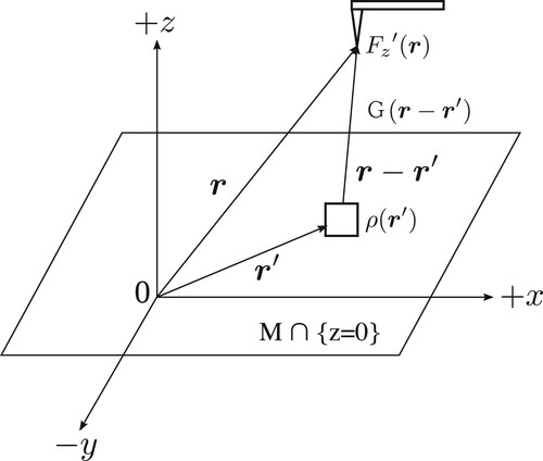This problem is a discretization of the problem of solving integral equation (2(2) $F_z^{\prime }\left(r\right)=\left(\mathcal{G}\rho \right)\left(r\right):={\int }_{M}G(r-r^{\prime })\rho \left(r^{\prime }\right)d{r}^{\prime },$(2) ). This integral-equation formulation is based on [4]. The anisotropic permanent magnet sample is denoted by M. Figure 1 shows the three-dimensional MFM tip Green function $G\left(r\right)$ $(r=(x,y,z)\in {\mathbb{R}}^3)$ for a dipole type MFM tip, and the rectangle is $M\cap \{z=0\}.$ Here, we consider the Green function for a point magnetic charge. The magnetization for the dipole type MFM tip is regarded as an infinitesimal magnetic dipole moment, which gives the maximum spatial resolution. In Figure 1, the z-axis represents the normal direction to the surface of the sample M. Let $F_z^{\prime }\left(r\right)$ denote the magnetic force gradient along the z direction at the position r, that is, $F_z^{\prime }\left(r\right)$ is an $\mathbb{R}$-valued function corresponding to the signal amplitude of an MFM image at r. Then, $F_z^{\prime }\left(r\right)$ is given by the convolution integral of the point magnetic charge distribution $\rho \left(r\right)$ with $G\left(r\right)$ as (2) $F_z^{\prime }\left(r\right)=\left(\mathcal{G}\rho \right)\left(r\right):={\int }_{M}G(r-r^{\prime })\rho \left(r^{\prime }\right)d{r}^{\prime },$(2) where $r^{\prime }=(x^{\prime },y^{\prime },z^{\prime })$ runs through sample M, $r^{\prime }\in M,$ and $d{r}^{\prime }=d{x}^{\prime }d{y}^{\prime }d{z}^{\prime }.$ Let $m=(m_x,m_y,m_z)$ denote the magnetization of the MFM tip. In a real situation, both the magnetization components $m_x$ and $m_y$ are 0. In the following, we normalize $m_z/4\pi {\mu }_0$ to 1, where ${\mu }_0$ denotes the vacuum permeability. Then, $G\left(r\right)$ is represented by (3) $G\left(r\right)=\frac{15z^3-9z\left(x^2+y^2+z^2\right)}{{\left(x^2+y^2+z^2\right)}^{7/2}}.$(3) Note that $G(r-r^{\prime })$ does not become ∞ because the MFM tip is far from the magnetic sample. Our (infinite-degrees-of-freedom) inverse problem requires determining the unknown distribution ρ from the observation data $F_z^{\prime }.$

Figure 1. MFM.

2.2. Simple discretization

Integral Equation (2(2) $F_z^{\prime }\left(r\right)=\left(\mathcal{G}\rho \right)\left(r\right):={\int }_{M}G(r-r^{\prime })\rho \left(r^{\prime }\right)d{r}^{\prime },$(2) ) is a linear Fredholm equation of the first kind. In general, the solution ρ is not unique for given data $F_z^{\prime }$ (see [2,3]). In this study, as described in Section 1, we consider the following basic and ideal discretized problem of Equation (2(2) $F_z^{\prime }\left(r\right)=\left(\mathcal{G}\rho \right)\left(r\right):={\int }_{M}G(r-r^{\prime })\rho \left(r^{\prime }\right)d{r}^{\prime },$(2) ) as a model problem of (1(1) $\text{estimate }\mu \in \mathcal{M}\text{ from observation data }f=T_{\delta }\left(\mu \right):=T\left(\mu \right)+\delta ,$(1) ).

1. All magnetic samples are cuboids of the same size (see Remark 2.1).

2. Every magnetic sample is always on the same horizontal plane, and all the observation points are common to all samples.

3. The MFM probe tip can be considered as a point magnetic dipole.

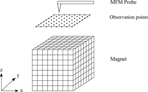
4. Every magnetic sample is divided into small cubic cells as in Figure 2; we call it cell discretization. Each cell or a set of several cells is a magnetic grain with single magnetic domain structure. (Although it is false if the boundary of a magnetic grain cuts the cell, we consider that it is limited to this case (see Experimental claim 4.3).) Every magnetic grain is magnetically isolated from the neighbouring magnetic grains by the non-magnetic boundary phase.

5. The length of each side of every cubic cell is normalized to 1.

6. The normalized value of the magnetic moment is 1 (upward) or $-1$ (downward) in each cell. (When a magnetic grain comprises several cells, the moments of those cells are oriented in the same direction.)

Remark 2.1

Further, if we discretize the space around the magnetic sample into cells, we do not need assumption (i). Then, assumption (ii) is ‘the normalized value of the magnetic moment is 1 (upward), $-1$ (downward), or 0 (space) in each cell’. In this case, the estimation is more difficult than in the case of assumption (i) because the estimation is to select one out of three possibilities. However, it is known which cells are included in the space, that is, which cells have the 0-value moment. The difficulty is mitigated if the information can be used for estimation.

Figure 2. Cell discretization.

We let $n_{\mu },n_x,n_y$ and $n_z$ denote the total number of cells, the number of cells in the x-axis direction, in the y-axis direction and in the z-axis direction, respectively. Therefore, $n_{\mu }=n_x{n}_y{n}_z,$ and the cells can be numbered as $c_1,\dots ,c_{n_z},$ $c_{n_z+1},\dots ,c_{n_z+n_z},c_{2n_z+1},\dots ,c_{2n_z+n_z},\dots ,c_{(n_x{n}_y-1)n_z+1},\dots ,c_{(n_x{n}_y-1)n_z+n_z}.c_{2n_z+1},\dots ,c_{2n_z+n_z},\dots ,c_{(n_x{n}_y-1)n_z+1},\dots ,c_{(n_x{n}_y-1)n_z+n_z}.c_{2n_z+1},\dots ,c_{2n_z+n_z},\dots ,c_{(n_x{n}_y-1)n_z+1},\dots ,c_{(n_x{n}_y-1)n_z+n_z}$. Here, suffix $i=a{n}_z+b$ $(a=0,\dots ,n_x{n}_y-1,b=1,\dots ,n_z)$ means that the position of the cell is ath in the horizontal (x –y plane) direction and bth in the vertical direction from the top. (The order in the horizontal direction is determined appropriately.)

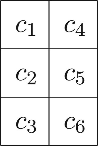
Example 2.2

We consider the case of $n_{\mu }=6,$ $n_x=2,$ $n_y=1,$ and $n_z=3.$ Then, the numbering of cells is as shown in Figure 3.

Figure 3. Numbering cells.

Let ${\mu }_i$ denote the magnetic moment of cell $c_i;$ then, ${\mu }_i=1$ (upward) or ${\mu }_i=-1$ (downward). We consider the magnetic charge of each cell, which is determined from its moment. If ${\mu }_i=1,$ then the values of charges are 1 and $-1$ at the top and bottom faces of cell $c_i,$ respectively. If ${\mu }_i=-1,$ then the values of charges are $-1$ and 1 at the top and bottom faces of cell $c_i,$ respectively. The values of charges are zero inside each cell and at all vertical faces of each cell. In addition to assumption (vi), we assume

(vii)

The values of the charge of the top/bottom face are centred at the centre point of the top/bottom face.

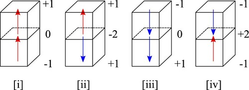
Next, we consider two vertically adjacent cells. The centre points of adjacent faces of these two cells are the same, and the value of the magnetic charge at this point is the sum of the values at the two adjacent centre points. Thus the value is $-2$, 0 or 2. Therefore, when the cell-discretized magnetic sample M comprises only two vertically adjacent cells, the possible values of charges are $-2$, $-1$, 0, 1 and 2. Figure 4 illustrates the magnetic moments (up or down arrows) and charges in the four possible cases. Next, we consider the general case. By identifying overlapping points, the total number of the centre points of the top and bottom faces of all cells is given by $n_{\rho }:=n_x{n}_y(n_z+1).$ These points can be numbered as $p_1,\dots ,p_{n_z+1},$ $p_{(n_z+1)+1},\dots ,p_{(n_z+1)+(n_z+1)},$ $p_{2(n_z+1)+1},\dots ,p_{2(n_z+1)+(n_z+1)},$ …, $p_{(n_x{n}_y-1)(n_z+1)+1},\dots ,p_{(n_x{n}_y-1)(n_z+1)+(n_z+1)}.$ Here, suffix $j=a(n_z+1)+b$ of $p_j$ $(a=0,\dots ,n_x{n}_y-1,b=1,\dots ,n_z+1)$ means that the position of the charge is ath in the horizontal (x –y plane) direction and bth in the vertical direction from the top. The order in the horizontal direction is the same as that of the cells. Let ${\rho }_j$ denote the magnetic charge at $p_j.$ Then, ${\rho }_j=-2,-1,0,1$ or 2.

Figure 4. Magnetic moments and charges.

Let $n_o$ denote the number of the observation points, where we observe the values of $F_z^{\prime }$ at these points. We number these points appropriately as $o_1,o_2,\dots ,o_{n_o},$ and we let $f_k$ denote the value of $F_z^{\prime }\left(r\right)$ at $o_k.$ Next, we define (4) $g_{kj}:=G(o_k-p_j).$(4) This is a discretization of (3(3) $G\left(r\right)=\frac{15z^3-9z\left(x^2+y^2+z^2\right)}{{\left(x^2+y^2+z^2\right)}^{7/2}}.$(3) ). Put $f:=\left[\begin{array}{c}{f}_1\\ f_2\\ ⋮\\ f_{n_o}\end{array}\right],G:=\left[\begin{array}{ccc}{g}_{11}& \cdots & g_{1n_{\rho }}\\ g_{21}& \cdots & g_{2n_{\rho }}\\ ⋮& ⋮& ⋮\\ g_{n_{o}1}& \cdots & g_{n_o{n}_{\rho }}\end{array}\right],\rho :=\left[\begin{array}{c}{\rho }_1\\ {\rho }_2\\ ⋮\\ {\rho }_{n_{\rho }}\end{array}\right].$Thus, we have a discretized equation of (2(2) $F_z^{\prime }\left(r\right)=\left(\mathcal{G}\rho \right)\left(r\right):={\int }_{M}G(r-r^{\prime })\rho \left(r^{\prime }\right)d{r}^{\prime },$(2) ), (5) $f=G\rho .$(5)

The relationship between ${\mu }_i$ and ${\rho }_j$ is as follows. Put $R:=\left[\begin{array}{cccc}{R}_1& 0& \cdots & 0\\ 0& R_2& \cdots & 0\\ ⋮& ⋮& \ddots & ⋮\\ 0& 0& \cdots & R_{n_x{n}_y}\end{array}\right],\mu :=\left[\begin{array}{c}{\mu }_1\\ {\mu }_2\\ ⋮\\ {\mu }_{n_{\mu }}\end{array}\right],$where ${\mu }_i$ denotes the moment of $c_i$ $(i=1,\dots ,n_{\mu })$ and $R_1,\dots ,R_{n_x{n}_y}$ are $(n_z+1)\times n_z$ matrices such that $R_1=\cdots =R_{n_x{n}_y}=\left[\begin{array}{ccccccc}1& 0& 0& \cdots & 0& 0& 0\\ -1& 1& 0& \cdots & 0& 0& 0\\ 0& -1& 1& \cdots & 0& 0& 0\\ ⋮& ⋮& & & & ⋮& ⋮\\ 0& 0& 0& \cdots & -1& 1& 0\\ 0& 0& 0& \cdots & 0& -1& 1\\ 0& 0& 0& \cdots & 0& 0& -1\end{array}\right].$Then, we have $\rho =R\mu .$ Thus our discretized (noiseless) inverse problem is now to solve the following system of linear equations: (6) $GR\mu =f.$(6) This equation is the same as Equation (1(1) $\text{estimate }\mu \in \mathcal{M}\text{ from observation data }f=T_{\delta }\left(\mu \right):=T\left(\mu \right)+\delta ,$(1) ) with $m=n_{\mu },$ $n=n_o,$ $T=GR,$ and $\delta =0.$ Since each ${\mu }_i$ is either 1 or $-1,$ the total number of possible patterns that μ can take is $2^{n_{\mu }}.$ Let $\mathcal{M}$ be the set of the all patterns, that is, $\mathcal{M}=\left\{\mu :\text{ each }{\mu }_i\text{ is 1 or }-1\right\}=\{-1,1{\}}^{n_{\mu }}.$Then, GR is a map from $\mathcal{M}\subset {\mathbb{R}}^{n_{\mu }}$ to ${\mathbb{R}}^{n_o}.$ We call $\mu \in \mathcal{M}$ a moment vector. Since $\mathcal{M}$ is a finite set, GR may have the inverse map even if $\dim n_o<\dim n_{\mu }.$

We consider the discretized inverse problem (6(6) $GR\mu =f.$(6) ) under assumption (i)–(vii); however, the original inverse problem is (2(2) $F_z^{\prime }\left(r\right)=\left(\mathcal{G}\rho \right)\left(r\right):={\int }_{M}G(r-r^{\prime })\rho \left(r^{\prime }\right)d{r}^{\prime },$(2) ). In the rest of this subsection, we consider the relationship between these two problems. Let $O\subset {\mathbb{R}}^3$ denote an observation area, that is, O is an area containing all the observation points. In Figure 2, O is a two-dimensional square. Let $\parallel \cdot {\parallel }_O$ and $\parallel \cdot {\parallel }_M$ denote appropriate norms of a function defined on O and M, respectively, e.g. they are the $L^2$ norms. Then, for Equation (2(2) $F_z^{\prime }\left(r\right)=\left(\mathcal{G}\rho \right)\left(r\right):={\int }_{M}G(r-r^{\prime })\rho \left(r^{\prime }\right)d{r}^{\prime },$(2) ), there exists C > 0 such that $\parallel F_z^{\prime }{\parallel }_O=\parallel \mathcal{G}\rho {\parallel }_O\le C\parallel \rho {\parallel }_M$for every ρ because $G(r-r^{\prime })$ $(r\in O,r^{\prime }\in M)$ is bounded on $O\times M.$ Only in the rest of this subsection, we denote the length of each side of every cell by Δ and write ${\rho }_{\mathrm{\Delta }}$ as ρ, $G_{\mathrm{\Delta }}$ as G, and $f_{\mathrm{\Delta }}$ as f in the discretized Equation (5(5) $f=G\rho .$(5) ). We can consider that the vectors $f_{\mathrm{\Delta }}$ and ${\rho }_{\mathrm{\Delta }}$ are piecewise constant functions defined on O and M, respectively. (Note that the components of these vectors are labelled with $n_o$ points in O and $n_{\rho }$ points in M, respectively.) Then, we have $\parallel F_z^{\prime }-\mathcal{G}{\rho }_{\mathrm{\Delta }}{\parallel }_O=\parallel \mathcal{G}\rho -\mathcal{G}{\rho }_{\mathrm{\Delta }}{\parallel }_O\le C\parallel \rho -{\rho }_{\mathrm{\Delta }}{\parallel }_M$and $\parallel \mathcal{G}{\rho }_{\mathrm{\Delta }}-f_{\mathrm{\Delta }}{\parallel }_O=\parallel \mathcal{G}{\rho }_{\mathrm{\Delta }}-G_{\mathrm{\Delta }}{\rho }_{\mathrm{\Delta }}{\parallel }_O\le \parallel \mathcal{G}-G_{\mathrm{\Delta }}\parallel \parallel {\rho }_{\mathrm{\Delta }}{\parallel }_M,$where $\parallel \mathcal{G}-G_{\mathrm{\Delta }}\parallel$ is the operator norm of $\mathcal{G}-G_{\mathrm{\Delta }}.$ Note that $\parallel \mathcal{G}-G_{\mathrm{\Delta }}\parallel \to 0$ as $\mathrm{\Delta }\to 0$ because the integral kernel of $\mathcal{G}$ is smooth, and there exists $C^{\prime }>0$ such that $\parallel {\rho }_{\mathrm{\Delta }}{\parallel }_M<C^{\prime }$ for every $\mathrm{\Delta }>0$ because $|{\rho }_j|\le 2.$ Therefore, by using $\parallel F_z^{\prime }-f_{\mathrm{\Delta }}{\parallel }_O\le \parallel F_z^{\prime }-\mathcal{G}{\rho }_{\mathrm{\Delta }}{\parallel }_O+\parallel \mathcal{G}{\rho }_{\mathrm{\Delta }}-f_{\mathrm{\Delta }}{\parallel }_O,$ we have a stability property: $f_{\mathrm{\Delta }}\to F_z^{\prime }$ as $\mathrm{\Delta }\to 0$ and ${\rho }_{\mathrm{\Delta }}\to \rho .$ This stability property ensures the validity of the discretized approximation of the ‘forward’ problem, that is, the problem of determining $F_z^{\prime }$ from ρ. However, our inverse problem does not have such a stability property. We consider this in Section 4.2.

2.3. Selection of pieces of $\mathcal{M}$

In Section 1, we introduced the concept of a piece of $\mathcal{M}.$ Each piece of $\mathcal{M}$ is a subset of $\mathcal{M},$ and the sum of all pieces is $\mathcal{M}.$ It is important to select pieces appropriately for problem (1(1) $\text{estimate }\mu \in \mathcal{M}\text{ from observation data }f=T_{\delta }\left(\mu \right):=T\left(\mu \right)+\delta ,$(1) ). The properties that pieces are expected to satisfy are described in Sections 3.2 and 3.3. For the inverse problem (6(6) $GR\mu =f.$(6) ), the following pieces (i.e. subsets) of $\mathcal{M}$ can be naturally obtained.

For a moment vector $\mu =[{\mu }_1,\dots ,{\mu }_{n_{\mu }}{]}^t\in \mathcal{M}$ ($[\cdot {]}^t$ denotes the transpose) defined in Section 2.2 and $\ell =1,2,\dots ,n_z,$ define ${\mu }_{\left[\ell \right]}={\left[{\mu }_{\left[\ell \right],1},{\mu }_{\left[\ell \right],2},\dots ,{\mu }_{\left[\ell \right],n_{\mu }}\right]}^t\in {\mathbb{R}}^{n_{\mu }}$by ${\mu }_{\left[\ell \right],i}:=\left\{\begin{array}{ll}{\mu }_i,& \text{if }i=\ell ,n_z+\ell ,2n_z+\ell ,\dots ,(n_x{n}_y-1)n_z+\ell \\ 0,& \text{otherwise.}\end{array}\right.$Consequently, the ith component of ${\mu }_{\left[\ell \right]}$ is equal to the ith component of μ if the component is the magnetic moment of one of the ℓth cells vertically from the top of M, and otherwise, the ith component of ${\mu }_{\left[\ell \right]}$ is 0. For example, the non-zero components of ${\mu }_{\left[1\right]}$ correspond to the cells of the top surface of M. (Furthermore, see Example 2.3.) We define ${\mathcal{M}}_{\left[\ell \right]}:=\left\{{\mu }_{\left[\ell \right]}:\mu \in \mathcal{M}\right\}\subset {\mathbb{R}}^{n_{\mu }}(\ell =1,2,\dots ,n_z)$and we call ${\mathcal{M}}_{\left[\ell \right]}$ the ℓth piece of $\mathcal{M}.$ In particular, ${\mathcal{M}}_{\left[1\right]}$ and ${\mathcal{M}}_{\left[\overline{m}\right]}$ are called the top piece and the bottom piece, respectively. Furthermore, ${\mathcal{M}}_{\left[\ell \right]}$ with a small value of ℓ is called an upper piece while ${\mathcal{M}}_{\left[\ell \right]}$ with a large value of ℓ is called a lower piece. Then, we have (7) $\mu =\sum _{\ell =1}^{n_z}{\mu }_{\left[\ell \right]}.$(7) There exists a natural projection $\mathcal{M}=\left\{\mu =\sum _{\ell =1}^{n_z}{\mu }_{\left[\ell \right]}:{\mu }_{\left[\ell \right]}\in {\mathcal{M}}_{\left[\ell \right]}\right\}⟵\underset{\ell =1}{\overset{n_z}{⨁}}{\mathcal{M}}_{\left[\ell \right]}\subset \underset{\ell =1}{\overset{n_z}{⨁}}{\mathbb{R}}^{n_{\mu }},$where the symbol ⊕ denotes the direct sum of vector spaces or their subsets. However, ${\mathcal{M}}_{\left[\ell \right]}\subset \mathcal{M}$ does not hold because μ does not have zero components and ${\mu }_{\left[\ell \right]}$ has zero components.

Example 2.3

We consider the case of Example 2.2. The cells $\{c_1,c_2,\dots ,c_6\}$ corresponding to the elements $[{\mu }_1,{\mu }_2,\dots ,{\mu }_6{]}^t$ are as shown in Figure 3. Then, for $\mu =[{\mu }_1,{\mu }_2,\dots ,{\mu }_6{]}^t,$ we have ${\mu }_{\left[1\right]}=[{\mu }_1,0,0,{\mu }_4,0,0{]}^t,$ ${\mu }_{\left[2\right]}=[0,{\mu }_2,0,0,{\mu }_5,0{]}^t,$ and ${\mu }_{\left[3\right]}=[0,0,{\mu }_3,0,0,{\mu }_6{]}^t.$ In this case, the sets of cells corresponding to nonzero components of ${\mathcal{M}}_{\left[1\right]},$ ${\mathcal{M}}_{\left[2\right]},$ and ${\mathcal{M}}_{\left[3\right]}$ are $\{c_1,c_4\},$ $\{c_2,c_5\},$ and $\{c_3,c_6\},$ respectively.

In the following, we often identify a piece with the set of cells corresponding to it.

3. Inverse problem with a linear forward operator and a sequential estimation-removal method

In this section, we consider the general inverse problems of the form (1(1) $\text{estimate }\mu \in \mathcal{M}\text{ from observation data }f=T_{\delta }\left(\mu \right):=T\left(\mu \right)+\delta ,$(1) ).

3.1. Inverse problem with a linear forward operator

Let $m,n,$ T, $\tilde{T}$ and $\mathcal{M}\subset {\mathbb{R}}^m$ be the integers, operators and set as described in Section 1. In the following, we aim to develop an estimation method for the inverse problems of the form (1(1) $\text{estimate }\mu \in \mathcal{M}\text{ from observation data }f=T_{\delta }\left(\mu \right):=T\left(\mu \right)+\delta ,$(1) ) with $\text{Ker }\tilde{T}\ne \left\{0\right\}$ and $\delta \ne 0.$ Since $\mathcal{M}$ is a finite set, $T:\mathcal{M}\to {\mathbb{R}}^n$ may be injective even if $\text{Ker }\tilde{T}\ne \left\{0\right\}.$ Then, the inverse map $T^{-1}:T\left(\mathcal{M}\right)\to \mathcal{M}$ exists. However, it is often nonlinear as per the following lemma.

Lemma 3.1

Let L and $L^{\prime }$ be the linear subspaces spanned by $\mathcal{M}$ and $T\left(\mathcal{M}\right),$ respectively. Assume that $L\cap \text{Ker }\tilde{T}\ne \left\{0\right\}$ and $T:\mathcal{M}\to T\left(\mathcal{M}\right)$ is injective. Then, $T^{-1}:T\left(\mathcal{M}\right)\to \mathcal{M}$ cannot be extended to a linear map $L^{\prime }\to L.$

Proof.

Since $T:L\to L^{\prime }$ is linear, we have $\dim L^{\prime }\le \dim L.$ If $T^{-1}:T\left(\mathcal{M}\right)\to \mathcal{M}$ has a linear extension, we have $\dim L^{\prime }\ge \dim L.$ Therefore, $\dim L^{\prime }=\dim L.$ Then, $\tilde{T}:L\to L^{\prime }$ is also injective. Hence, $L\cap \text{Ker }\tilde{T}=\left\{0\right\}.$ This contradicts the assumption that $L\cap \text{Ker }\tilde{T}\ne \left\{0\right\}.$

Even if T is not injective, there may exist subsets ${\mathcal{M}}_I,{\mathcal{M}}_C$ of ${\mathbb{R}}^m$ such that every $\mu \in \mathcal{M}$ has a unique decomposition of the form: $\mu ={\mu }_I+{\mu }_C,{\mu }_I\in {\mathcal{M}}_I,{\mu }_C\in {\mathcal{M}}_C$and ${\mu }_I$ can be uniquely determined by $T\left(\mu \right).$ For simplicity, we denote the map (8) $T\left(\mathcal{M}\right)⟶{\mathcal{M}}_I,T\left(\mu \right)=T\left({\mu }_I\right)+T\left({\mu }_C\right)⟼{\mu }_I$(8) by $T^{-1}.$ In general, the map $T\left({\mu }_I\right)\mapsto {\mu }_I$ is also nonlinear. The set of all the vectors of the form of (15(15) $\sum _{\ell =1}^{\overline{\overline{m}}}{\mu }_{\left[\ell \right]},$(15) ) below is an example of ${\mathcal{M}}_I$ (if $\delta =0).$

From Section 4 onward, we consider the (discretized) magnetization-distribution identification problem described in Section 2. It is an example of the above-mentioned inverse problem. In this problem, $\mathcal{M}=\{-1,1{\}}^m$ and (practically) $\text{Ker }\tilde{T}\ne \left\{0\right\}.$ However, in some cases, the inverse map $T^{-1}$ exists and it is (practically) nonlinear. (The linear space L spanned by $\mathcal{M}$ is ${\mathbb{R}}^m.$ Therefore, $L\cap \text{Ker }\tilde{T}\ne \left\{0\right\},$ and the nonlinearity of $T^{-1}:T\left(\mathcal{M}\right)\to \mathcal{M}$ is obtained using Lemma 3.1.) Therefore, it is difficult to solve the inverse problem by employing a linear algebra method. We aim to construct a map N that approximates $T^{-1},$ $N\approx T^{-1},$ for example, by machine learning (deep learning). Further, this map N is expected to be as robust as possible to noise.

3.2. A sequential estimation-removal method

Machine learning is often computationally expensive. In the numerical experiments conducted on our magnetic inverse problem, the deep learning for constructing a neural network, $N\approx T^{-1},$ stopped before the value of the loss function becomes small enough. (One of the reasons we think is described in Section 3.4.) Therefore, we divide the problem as follows. Let $\overline{m}\in \mathbb{N},$ $\overline{m}\le m$ and ${\mathcal{M}}_{\left[1\right]},{\mathcal{M}}_{\left[2\right]},\dots ,{\mathcal{M}}_{\left[\overline{m}\right]}$ be subsets of ${\mathbb{R}}^m$ such that, every $\mu \in \mathcal{M}$ has a unique decomposition of the form: (9) $\mu =\sum _{\ell =1}^{\overline{m}}{\mu }_{\left[\ell \right]}\left({\mu }_{\left[\ell \right]}\in {\mathcal{M}}_{\left[\ell \right]}\right),$(9) where $\sum$ denotes the sum of vectors in ${\mathbb{R}}^m$ (see (7(7) $\mu =\sum _{\ell =1}^{n_z}{\mu }_{\left[\ell \right]}.$(7) )). As described in Section 2.3, there exists a natural projection $\mathcal{M}=\left\{\sum _{\ell =1}^{n_z}{\mu }_{\left[\ell \right]}:{\mu }_{\left[\ell \right]}\in {\mathcal{M}}_{\left[\ell \right]}\right\}⟵\underset{\ell =1}{\overset{\overline{m}}{⨁}}{\mathcal{M}}_{\left[\ell \right]}.$However, ${\mathcal{M}}_{\left[\ell \right]}\subset \mathcal{M}$ may not hold, and we call ${\mathcal{M}}_{\left[\ell \right]}$ the ℓth piece of $\mathcal{M}.$

If T is injective, there exists the inverse map N, i.e. $N\left(T\right(\mu \left)\right)=\mu .$ Therefore, we can consider maps $N_{\left[1\right]},N_{\left[2\right]},\dots ,N_{\left[\overline{m}\right]}$ such that $N_{\left[\ell \right]}\left(T\right(\mu \left)\right)={\mu }_{\left[\ell \right]}.$Moreover, for $f=T_{\delta }\left(\mu \right)=T\left(\mu \right)+\delta$ with $\text{Ker }\tilde{T}\ne \left\{0\right\},$ it may be expected that the following holds: $N_{\left[\ell \right]}\left(f\right)=N_{\left[\ell \right]}\left(T_{\delta }\left(\mu \right)\right)\approx {\mu }_{\left[\ell \right]}.$If we have these maps, we can estimate μ as $\mu \approx \sum _{\ell =1}^{\overline{m}}{N}_{\left[\ell \right]}\left(f\right).$This method independently estimates ${\mu }_{\left[1\right]},{\mu }_{\left[2\right]},\dots ,{\mu }_{\left[\overline{m}\right]}$ and does not require the linearity of T. In the numerical experiments on our ill-posed magnetic inverse problem, this method was superior to the above-mentioned method that estimates μ at once. However, its performance was considerably inadequate even if $\delta =0.$ Therefore, we propose a reconstruction method (sequential estimation-removal method) based on the following idea:

Basic idea 3.2: A piece that can be accurately estimated should be estimated earlier.

In this method, we employ the linearity of T to solve the inverse problem (1(1) $\text{estimate }\mu \in \mathcal{M}\text{ from observation data }f=T_{\delta }\left(\mu \right):=T\left(\mu \right)+\delta ,$(1) ).

Let $\parallel \cdot {\parallel }_O$ denote a norm on ${\mathbb{R}}^n.$ To realize Basic idea 3.2, we expect that the pieces ${\mathcal{M}}_{\left[1\right]},{\mathcal{M}}_{\left[2\right]},\dots ,{\mathcal{M}}_{\left[\overline{m}\right]}$ are selected such that the value of $\parallel T\left({\mu }_{\left[\ell \right]}\right){\parallel }_O$ decreases as the value of ℓ increases. First, we expect that the selection satisfies (10) ${∥T\left({\mu }_{[\ell +1]}\right)∥}_O<{∥T\left({\mu }_{\left[\ell \right]}\right)∥}_O$(10) for all $\mu \in \mathcal{M}$ and $\ell =1,\dots ,\overline{m}-1.$ We call this property piece monotonicity. If this property cannot be obtained, we expect the following property holds:

• For every $\mu \in \mathcal{M}$ and every $\ell =1,\dots ,\overline{m},$ it holds that $\dim {\mu }_{\left[\ell \right]}=m/\overline{m}.$ (In our magnetic inverse problem, this implies that every piece corresponds to the same number of cells.)

•  (10(10) ${∥T\left({\mu }_{[\ell +1]}\right)∥}_O<{∥T\left({\mu }_{\left[\ell \right]}\right)∥}_O$(10) ) holds if ${\mu }_{\left[\ell \right]}={\mu }_{[\ell +1]}$ as $m/\overline{m}$-dimensional vectors, where the order of the elements is properly determined (see Example 3.3).

We call this property weak piece monotonicity. As described in Section 2.3, we call ${\mathcal{M}}_{\left[\ell \right]}$ with a small value of ℓ an upper piece while ${\mathcal{M}}_{\left[\ell \right]}$ with a large value of ℓ a lower piece. In particular, ${\mathcal{M}}_{\left[1\right]}$ and ${\mathcal{M}}_{\left[\overline{m}\right]}$ are called the top piece and the bottom piece, respectively. To realize Basic idea 3.2, we expect that a piece closer to the top piece can be estimated more accurately. In Section 4.3, it is experimentally shown that the pieces obtained in Section 2.3 for our magnetic inverse problem satisfy piece monotonicity for $\ell =1,\dots ,m^{\prime }$ with some $m^{\prime }$ $\le \overline{m}=10$ (see Table 7) and weak piece monotonicity for $\ell =1,\dots ,\overline{m}=10$ (see Table 9). In Assumption 3.5, we will describe other properties that pieces are expected to satisfy, and in Section 3.3, we will describe some conditions for Assumption 3.5 to hold.

Example 3.3

We consider the case of the discretized magnetization-distribution identification problem described in Section 2. For example, in the same case of $m=n_{\mu }=6$ and $\overline{m}=n_z=3$ as in Examples 2.2 and 2.3, we consider ${\mu }_{\left[1\right]}=[1,0,0,-1,0,0{]}^t,$ ${\mu }_{\left[2\right]}=[0,1,0,0,-1,0{]}^t,$ and ${\mu }_{\left[3\right]}=[0,0,1,0,0,-1{]}^t$ to be equal to each other as $2(=m/\overline{m})$-dimensional vectors.

We consider a reconstruction method based on Basic idea 3.2. First, we consider the case where $\text{Ker }\tilde{T}=\left\{0\right\}$ and $\delta =0,$ that is, the well-posed case. For $\mu \in \mathcal{M}$ and ${\mu }_{\left[\ell \right]}\in {\mathcal{M}}_{\left[\ell \right]}$ $(\ell =1,2,\dots ,\overline{m})$ given by (9(9) $\mu =\sum _{\ell =1}^{\overline{m}}{\mu }_{\left[\ell \right]}\left({\mu }_{\left[\ell \right]}\in {\mathcal{M}}_{\left[\ell \right]}\right),$(9) ), we define ${\mu }_{\left[\ell \right]\downarrow }:=\sum _{k=\ell }^{\overline{m}}{\mu }_{\left[k\right]},f_{\left[\ell \right]}:=T\left({\mu }_{\left[\ell \right]}\right),f_{\left[\ell \right]\downarrow }:=\sum _{k=\ell }^{\overline{m}}{f}_{\left[k\right]}.$Then, ${\mu }_{\left[1\right]\downarrow }=\mu .$ Using the linearity of T, we have, for $\ell =1,\dots ,\overline{m},$ $T\left({\mu }_{\left[\ell \right]\downarrow }\right)=\sum _{k=\ell }^{\overline{m}}T\left({\mu }_{\left[k\right]}\right)=\sum _{k=\ell }^{\overline{m}}{f}_{\left[k\right]}=f_{\left[\ell \right]\downarrow },$and then, $f_{\left[1\right]\downarrow }=f$ and $T^{-1}\left(f_{\left[\ell \right]\downarrow }\right)={\mu }_{\left[\ell \right]\downarrow }.$Therefore, for $\ell =1,2,\dots ,\overline{m},$ there exists $T_{\left[\ell \right]}^{-1}$ such that it outputs ${\mu }_{\left[\ell \right]}$ to the input $f_{\left[\ell \right]\downarrow },$ i.e. (11) $T_{\left[\ell \right]}^{-1}\left(f_{\left[\ell \right]\downarrow }\right)={\mu }_{\left[\ell \right]}={\left.{\mu }_{\left[\ell \right]\downarrow }\right|}_{{\mathcal{M}}_{\left[\ell \right]}}\left(\ell =1,2,\dots ,\overline{m}\right).$(11) Note that $T_{\left[\ell \right]}^{-1}$ does not give ${\mu }_{\left[\ell \right]\downarrow }$ but ${\mu }_{\left[\ell \right]}$ from $f_{\left[\ell \right]\downarrow }.$ Thus we can use $T_{\left[\ell \right]}^{-1}$ $(\ell =1,2,\dots ,\overline{m})$ to obtain μ from a given f by the following procedure.

Procedure 3.4

1. Put $\ell =1.$

2. Calculate ${\mu }_{\left[1\right]}=T_{\left[1\right]}^{-1}\left(f\right)\text{and}{f}_{\left[1\right]}=T\left({\mu }_{\left[1\right]}\right).$

3. $\ell \leftarrow \ell +1.$

4. Calculate (12) ${\mu }_{\left[\ell \right]}=T_{\left[\ell \right]}^{-1}\left(f_{\left[\ell \right]\downarrow }\right)=T_{\left[\ell \right]}^{-1}\left(f-\sum _{k=1}^{\ell -1}{f}_{\left[k\right]}\right),$(12) and if $\ell <\overline{m},$ calculate $f_{\left[\ell \right]}=T\left({\mu }_{\left[\ell \right]}\right).$

5. If $\ell =\overline{m},$ stop the procedure. Otherwise, go back to step 3.

This procedure outputs $\mu =\sum _{\ell =1}^{\overline{m}}{\mu }_{\left[\ell \right]}.$In this procedure, the pieces are estimated and removed one-by-one from the top. We call this method a sequential estimation-removal method.

In general, $\text{Ker }\tilde{T}$ may not be equal to $\left\{0\right\},$ and there exists some noise $\delta \ne 0$ in (1(1) $\text{estimate }\mu \in \mathcal{M}\text{ from observation data }f=T_{\delta }\left(\mu \right):=T\left(\mu \right)+\delta ,$(1) ). Therefore, we may not execute Procedure 3.4. In this case, we aim to obtain as much information regarding μ as possible. In the following, we assume that, for every $f=T_{\delta }\left(\mu \right)=T\left(\mu \right)+\delta ,$ there exists ${\delta }_{\left[\ell \right]\downarrow }\in {\mathbb{R}}^n$ such that $f_{\left[\ell \right]\downarrow }=T\left({\mu }_{\left[\ell \right]\downarrow }\right)+{\delta }_{\left[\ell \right]\downarrow }$ for $\ell =1,2,\dots ,\overline{m}.$ Set $\begin{array}{rl}{\mathcal{M}}_{\left[\ell \right]\downarrow }& :=\left\{\sum _{k=\ell }^{\overline{m}}{m}_{\left[k\right]}:m_{\left[k\right]}\in {\mathcal{M}}_{\left[k\right]}\right\}⟵\underset{k=\ell }{\overset{\overline{m}}{⨁}}{\mathcal{M}}_{\left[k\right]},\\ & \text{where the symbol }⟵\text{ means a natural projection,}\\ {\mathcal{F}}_{\left[\ell \right]\downarrow }& :=\left\{T\left(\nu \right):\nu \in {\mathcal{M}}_{\left[\ell \right]\downarrow }\right\},\\ {\mathrm{\Delta }}_{\left[\ell \right]\downarrow }& :=\left\{\eta \in {\mathbb{R}}^n:\text{possible noise for the elements of {}{\mathcal{F}}_{\left[\ell \right]\downarrow }\text{}}\right\},\\ {\mathcal{D}}_{\left[\ell \right]\downarrow }& :=\left\{T\left(\nu \right)+\eta :\nu \in {\mathcal{M}}_{\left[\ell \right]\downarrow },\eta \in {\mathrm{\Delta }}_{\left[\ell \right]\downarrow }\right\}.\end{array}$Then, ${\mathcal{F}}_{\left[\ell \right]\downarrow }$ and ${\mathcal{D}}_{\left[\ell \right]\downarrow }$ are the sets of components of the ℓth and lower pieces of all possible observation data values for the case where $\delta =0$ and $\delta \ne 0,$ respectively. We have ${\mathcal{M}}_{\left[1\right]\downarrow }=\mathcal{M},$ and set $\mathrm{\Delta }:={\mathrm{\Delta }}_{\left[1\right]\downarrow }.$ Here, considering that $\mathcal{M}$ is a finite set, we assume the following.

Assumption 3.5

1. (For the case where $\delta =0$)

   There exist $\overline{\overline{m}}\in \mathbb{N},$ $\overline{\overline{m}}\le \overline{m},$ and $T_{\left[\ell \right]}^{-1}:{\mathcal{F}}_{\left[\ell \right]\downarrow }\to {\mathcal{M}}_{\left[\ell \right]\downarrow }$ $(\ell =1,2,\dots ,\overline{\overline{m}})$ such that (13) $T_{\left[\ell \right]}^{-1}\left(f_{\left[\ell \right]\downarrow }\right)={\mu }_{\left[\ell \right]}$(13) holds for every $f=T\left(\mu \right)$ $(\mu \in \mathcal{M}).$

2. (For the case where $\delta \ne 0$)

   There exist $\overline{\overline{m}}\in \mathbb{N},$ $\overline{\overline{m}}\le \overline{m},$ and $T_{\left[\ell \right]}^{-1}:{\mathcal{D}}_{\left[\ell \right]\downarrow }\to {\mathcal{M}}_{\left[\ell \right]\downarrow }$ $(\ell =1,2,\dots ,\overline{\overline{m}})$ such that (14) $T_{\left[\ell \right]}^{-1}\left(f_{\left[\ell \right]\downarrow }\right)={\mu }_{\left[\ell \right]}$(14) holds for every $f=T_{\delta }\left(\mu \right)$ $(\mu \in \mathcal{M},\delta \in \mathrm{\Delta }).$

In this assumption, $\text{Ker }\tilde{T}$ may or may not be $\left\{0\right\}.$ If $\text{Ker }\tilde{T}=\left\{0\right\},$ Assumption 3.5 (i) always holds for $\overline{\overline{m}}=\overline{m}$ (see (11(11) $T_{\left[\ell \right]}^{-1}\left(f_{\left[\ell \right]\downarrow }\right)={\mu }_{\left[\ell \right]}={\left.{\mu }_{\left[\ell \right]\downarrow }\right|}_{{\mathcal{M}}_{\left[\ell \right]}}\left(\ell =1,2,\dots ,\overline{m}\right).$(11) )). $T_{\left[\ell \right]}^{-1}$ in (14(14) $T_{\left[\ell \right]}^{-1}\left(f_{\left[\ell \right]\downarrow }\right)={\mu }_{\left[\ell \right]}$(14) ) is an extension of $T_{\left[\ell \right]}^{-1}$ in (13(13) $T_{\left[\ell \right]}^{-1}\left(f_{\left[\ell \right]\downarrow }\right)={\mu }_{\left[\ell \right]}$(13) ) to the case where $\delta \ne 0.$ Based on Assumption 3.5, Procedure 3.4 can be rewritten as follows.

Procedure 3.6

Suppose that Assumption 3.5 is satisfied.

• Steps 1, 2 and 3 are the same steps in Procedure 3.4.

• Steps 4 and 5 are steps 4 and 5 in Procedure 3.4, where $\overline{m}$ is replaced by $\overline{\overline{m}}.$

This procedure does not output μ. Instead, it outputs (15) $\sum _{\ell =1}^{\overline{\overline{m}}}{\mu }_{\left[\ell \right]},$(15) that is, ${\mu }_{[\overline{\overline{m}}+1]},\dots ,{\mu }_{\left[\overline{m}\right]}$ cannot be estimated. Even when we define maps that estimate them in some sense, the estimated results may contain errors.

In the experiments in Sections 5 and 6, we use Procedure 3.4 even if $\overline{\overline{m}}<\overline{m}$ to test how deep (large ℓ) a piece our method can estimate. Deep learning in Section 5 and the iterative method in Section 6 can be formally applied even if $\overline{\overline{m}}<\overline{m}.$

3.3. Selection of pieces of $\mathcal{M}$

We consider piece monotonicity and weak piece monotonicity to be a naturally expected property of pieces to realize Basic idea 3.2. To execute Procedure 3.6, we must obtain pieces ${\mathcal{M}}_{\left[1\right]},$ …, ${\mathcal{M}}_{\left[\overline{\overline{m}}\right]}$ earlier and construct maps $T_{\left[1\right]}^{-1},$ …, $T_{\left[\overline{\overline{m}}\right]}^{-1}$ that satisfy Assumption 3.5. This assumption requires that the pieces satisfy some properties, which are somewhat different from (weak) piece monotonicity. This is considered here. Previous to it, we describe the stability/instability of the inverse problem (1(1) $\text{estimate }\mu \in \mathcal{M}\text{ from observation data }f=T_{\delta }\left(\mu \right):=T\left(\mu \right)+\delta ,$(1) ). We distinguish the elements of $\mathcal{M}$ with a superscript index as ${\mu }^{\left(\alpha \right)}.$ Let $\parallel \cdot {\parallel }_M$ denote a norm on ${\mathbb{R}}^m,$ and (16) $\begin{array}{rl}{r}^{\left(\alpha \text{β}\right)}& :=\frac{{∥T\left({\mu }^{\left(\alpha \right)}\right)-T\left({\mu }^{\left(\text{β}\right)}\right)∥}_O}{{∥{\mu }^{\left(\alpha \right)}-{\mu }^{\left(\text{β}\right)}∥}_M}(\alpha \ne \text{β}),\\ r^{min}& :=min\left\{r^{\left(\alpha \text{β}\right)}:{\mu }^{\left(\alpha \right)},{\mu }^{\left(\text{β}\right)}\in \mathcal{M},\alpha \ne \text{β}\right\}.\end{array}$(16) If $r^{min}>0,$ then the inverse problem (1(1) $\text{estimate }\mu \in \mathcal{M}\text{ from observation data }f=T_{\delta }\left(\mu \right):=T\left(\mu \right)+\delta ,$(1) ) with $\delta =0$ has a unique solution, and (17) ${∥{\mu }^{\left(\alpha \right)}-{\mu }^{\left(\text{β}\right)}∥}_M\le \frac{1}{r^{min}}{∥T\left({\mu }^{\left(\alpha \right)}\right)-T\left({\mu }^{\left(\text{β}\right)}\right)∥}_O$(17) holds for every ${\mu }^{\left(\alpha \right)}$ and ${\mu }^{\left(\text{β}\right)}.$ As the value of $r^{min}$ increases, the stability of the inverse problem (1(1) $\text{estimate }\mu \in \mathcal{M}\text{ from observation data }f=T_{\delta }\left(\mu \right):=T\left(\mu \right)+\delta ,$(1) ) increases. In fact, if ${\mu }^{\left(\alpha \right)}\ne {\mu }^{\left(\text{β}\right)}$ holds and $r^{min}$ is sufficiently large, then the values of $T\left({\mu }^{\left(\alpha \right)}\right)$ and $T\left({\mu }^{\left(\text{β}\right)}\right)$ are very different from each other.

For selecting pieces of $\mathcal{M},$ we consider a sufficient condition for Assumption 3.5 to hold (Lemma 3.8) and make the same consideration as above for each piece. Previously, we consider the following lemma that provides a sufficient condition for Assumption 3.5 (ii) to hold.

Lemma 3.7

Let $\ell \in \{1,2,\dots ,\overline{m}\}.$ Assume that (18) $2\underset{\eta \in {\mathrm{\Delta }}_{\left[\ell \right]\downarrow }}{sup}{∥\eta ∥}_O<{∥T\left({\mu }_{\left[\ell \right]\downarrow }^{\left(\alpha \right)}\right)-T\left({\mu }_{\left[\ell \right]\downarrow }^{\left(\text{β}\right)}\right)∥}_O$(18) is satisfied for ℓ and every ${\mu }^{\left(\alpha \right)},{\mu }^{\left(\text{β}\right)}\in \mathcal{M},$ $\alpha \ne \text{β}.$ Then, Assumption 3.5 (ii) holds for ℓ.

Proof.

Let $g=T\left({\mu }_{\left[\ell \right]\downarrow }\right)+{\delta }_{\left[\ell \right]\downarrow }$ $({\mu }_{\left[\ell \right]\downarrow }\in {\mathcal{M}}_{\left[\ell \right]\downarrow },{\delta }_{\left[\ell \right]\downarrow }\in {\mathrm{\Delta }}_{\left[\ell \right]\downarrow }).$ From (18(18) $2\underset{\eta \in {\mathrm{\Delta }}_{\left[\ell \right]\downarrow }}{sup}{∥\eta ∥}_O<{∥T\left({\mu }_{\left[\ell \right]\downarrow }^{\left(\alpha \right)}\right)-T\left({\mu }_{\left[\ell \right]\downarrow }^{\left(\text{β}\right)}\right)∥}_O$(18) ), we have that, for every ${\mu }^{\prime }\in \mathcal{M}$ with ${\mu }_{\left[\ell \right]}^{\prime }\ne {\mu }_{\left[\ell \right]},$ $\begin{array}{rl}& {∥T\left({\mu }_{\left[\ell \right]\downarrow }^{\prime }\right)-g∥}_O={∥T\left({\mu }_{\left[\ell \right]\downarrow }^{\prime }\right)-T\left({\mu }_{\left[\ell \right]\downarrow }\right)-{\delta }_{\left[\ell \right]\downarrow }∥}_O\\ & \ge {∥T\left({\mu }_{\left[\ell \right]\downarrow }^{\prime }\right)-T\left({\mu }_{\left[\ell \right]\downarrow }\right)∥}_O-{∥{\delta }_{\left[\ell \right]\downarrow }∥}_O>2\underset{\eta \in {\mathrm{\Delta }}_{\left[\ell \right]\downarrow }}{sup}{∥\eta ∥}_O-{∥{\delta }_{\left[\ell \right]\downarrow }∥}_O>{∥{\delta }_{\left[\ell \right]\downarrow }∥}_O.\end{array}$Further, ${∥T\left({\mu }_{\left[\ell \right]\downarrow }\right)-g∥}_O={∥{\delta }_{\left[\ell \right]\downarrow }∥}_O.$Thus we have ${\mu }_{\left[\ell \right]\downarrow }=\underset{\nu \in {\mathcal{M}}_{\left[\ell \right]\downarrow }}{\text{argmin}}{∥T\left(\nu \right)-g∥}_O.$Therefore, we can define $T_{\left[\ell \right]}^{-1}:{\mathcal{D}}_{\left[\ell \right]\downarrow }\to {\mathcal{M}}_{\left[\ell \right]\downarrow }$ by $\begin{array}{}& T_{\left[\ell \right]}^{-1}\left(g\right):={\left.\left(\underset{\nu \in {\mathcal{M}}_{\left[\ell \right]\downarrow }}{\text{argmin}}{∥T\left(\nu \right)-g∥}_O\right)\right|}_{{\mathcal{M}}_{\left[\ell \right]}}\end{array}$

The value of the left-hand side of (18(18) $2\underset{\eta \in {\mathrm{\Delta }}_{\left[\ell \right]\downarrow }}{sup}{∥\eta ∥}_O<{∥T\left({\mu }_{\left[\ell \right]\downarrow }^{\left(\alpha \right)}\right)-T\left({\mu }_{\left[\ell \right]\downarrow }^{\left(\text{β}\right)}\right)∥}_O$(18) ) is determined by noise. We separate the noise-independent part from (18(18) $2\underset{\eta \in {\mathrm{\Delta }}_{\left[\ell \right]\downarrow }}{sup}{∥\eta ∥}_O<{∥T\left({\mu }_{\left[\ell \right]\downarrow }^{\left(\alpha \right)}\right)-T\left({\mu }_{\left[\ell \right]\downarrow }^{\left(\text{β}\right)}\right)∥}_O$(18) ), that is, we consider an inequality for T that is similar to (17(17) ${∥{\mu }^{\left(\alpha \right)}-{\mu }^{\left(\text{β}\right)}∥}_M\le \frac{1}{r^{min}}{∥T\left({\mu }^{\left(\alpha \right)}\right)-T\left({\mu }^{\left(\text{β}\right)}\right)∥}_O$(17) ) for each piece in the following lemma. This is inequality (19(19) ${∥{\mu }_{\left[\ell \right]}^{\left(\alpha \right)}-{\mu }_{\left[\ell \right]}^{\left(\text{β}\right)}∥}_M\le C_{\left[\ell \right]}{∥T\left({\mu }_{\left[\ell \right]\downarrow }^{\left(\alpha \right)}\right)-T\left({\mu }_{\left[\ell \right]\downarrow }^{\left(\text{β}\right)}\right)∥}_O$(19) ). This inequality represents the difficulty of the estimation independent of noise.

Lemma 3.8

Let $\ell \in \{1,2,\dots ,\overline{m}\}.$ For ℓ, consider the conditions that there exists $C_{\left[\ell \right]}>0$ such that

1. it holds that (19) ${∥{\mu }_{\left[\ell \right]}^{\left(\alpha \right)}-{\mu }_{\left[\ell \right]}^{\left(\text{β}\right)}∥}_M\le C_{\left[\ell \right]}{∥T\left({\mu }_{\left[\ell \right]\downarrow }^{\left(\alpha \right)}\right)-T\left({\mu }_{\left[\ell \right]\downarrow }^{\left(\text{β}\right)}\right)∥}_O$(19) for every ${\mu }^{\left(\alpha \right)},{\mu }^{\left(\text{β}\right)}\in \mathcal{M},$

2. it holds that (20) $2C_{\left[\ell \right]}\underset{\eta \in {\mathrm{\Delta }}_{\left[\ell \right]\downarrow }}{sup}{∥\eta ∥}_O<{∥{\mu }_{\left[\ell \right]}^{\left(\alpha \right)}-{\mu }_{\left[\ell \right]}^{\left(\text{β}\right)}∥}_M$(20) for every ${\mu }^{\left(\alpha \right)},{\mu }^{\left(\text{β}\right)}\in \mathcal{M},$ $\alpha \ne \text{β}.$

Put $L:=\{1,2,\dots ,\overline{\overline{m}}\}.$ If and only if every $\ell \in L$ satisfies Lemma 3.8 (i), then Assumption 3.5 (i) holds. If every $\ell \in L$ satisfies Lemma 3.8 (i) and (ii), then Assumption 3.5 (ii) holds.

Proof.

The first case can be shown via a straightforward calculation. We show the second case. By employing (19(19) ${∥{\mu }_{\left[\ell \right]}^{\left(\alpha \right)}-{\mu }_{\left[\ell \right]}^{\left(\text{β}\right)}∥}_M\le C_{\left[\ell \right]}{∥T\left({\mu }_{\left[\ell \right]\downarrow }^{\left(\alpha \right)}\right)-T\left({\mu }_{\left[\ell \right]\downarrow }^{\left(\text{β}\right)}\right)∥}_O$(19) ) and (20(20) $2C_{\left[\ell \right]}\underset{\eta \in {\mathrm{\Delta }}_{\left[\ell \right]\downarrow }}{sup}{∥\eta ∥}_O<{∥{\mu }_{\left[\ell \right]}^{\left(\alpha \right)}-{\mu }_{\left[\ell \right]}^{\left(\text{β}\right)}∥}_M$(20) ), we have $2C_{\left[\ell \right]}\underset{\eta \in {\mathrm{\Delta }}_{\left[\ell \right]\downarrow }}{sup}{∥\eta ∥}_O<{∥{\mu }_{\left[\ell \right]}^{\left(\alpha \right)}-{\mu }_{\left[\ell \right]}^{\left(\text{β}\right)}∥}_M\le C_{\left[\ell \right]}{∥T\left({\mu }_{\left[\ell \right]\downarrow }^{\left(\alpha \right)}\right)-T\left({\mu }_{\left[\ell \right]\downarrow }^{\left(\text{β}\right)}\right)∥}_O.$Therefore, (18(18) $2\underset{\eta \in {\mathrm{\Delta }}_{\left[\ell \right]\downarrow }}{sup}{∥\eta ∥}_O<{∥T\left({\mu }_{\left[\ell \right]\downarrow }^{\left(\alpha \right)}\right)-T\left({\mu }_{\left[\ell \right]\downarrow }^{\left(\text{β}\right)}\right)∥}_O$(18) ) holds.

In Lemma 3.8, as the value of $C_{\left[\ell \right]}$ decreases, it becomes easier to distinguish between ${\mu }_{\left[\ell \right]}^{\left(\alpha \right)}$ and ${\mu }_{\left[\ell \right]}^{\left(\text{β}\right)}.$ To apply Lemma 3.8 to the inverse problem (1(1) $\text{estimate }\mu \in \mathcal{M}\text{ from observation data }f=T_{\delta }\left(\mu \right):=T\left(\mu \right)+\delta ,$(1) ), it is desirable for us to know the value of $min{C}_{\left[\ell \right]}.$ Define (21) $r_{\left[\ell \right]\downarrow }^{\left(\alpha \text{β}\right)}:=\frac{{∥T\left({\mu }_{\left[\ell \right]\downarrow }^{\left(\alpha \right)}\right)-T\left({\mu }_{\left[\ell \right]\downarrow }^{\left(\text{β}\right)}\right)∥}_O}{{∥{\mu }_{\left[\ell \right]}^{\left(\alpha \right)}-{\mu }_{\left[\ell \right]}^{\left(\text{β}\right)}∥}_M}(\alpha \ne \text{β})$(21) and (22) $r_{\left[\ell \right]}:=min\left\{r_{\left[\ell \right]\downarrow }^{\left(\alpha \text{β}\right)}:{\mu }_{\left[\ell \right]}^{\left(\alpha \right)},{\mu }_{\left[\ell \right]}^{\left(\text{β}\right)}\in {\mathcal{M}}_{\left[\ell \right]},\alpha \ne \text{β}\right\}.$(22) Then, if $r_{\left[\ell \right]}\ne 0,$ $min{C}_{\left[\ell \right]}=1/r_{\left[\ell \right]}$ holds and inequality (20(20) $2C_{\left[\ell \right]}\underset{\eta \in {\mathrm{\Delta }}_{\left[\ell \right]\downarrow }}{sup}{∥\eta ∥}_O<{∥{\mu }_{\left[\ell \right]}^{\left(\alpha \right)}-{\mu }_{\left[\ell \right]}^{\left(\text{β}\right)}∥}_M$(20) ) can be rewritten as (23) $\frac{2}{r_{\left[\ell \right]}}\underset{\eta \in {\mathrm{\Delta }}_{\left[\ell \right]\downarrow }}{sup}{∥\eta ∥}_O<{∥{\mu }_{\left[\ell \right]}^{\left(\alpha \right)}-{\mu }_{\left[\ell \right]}^{\left(\text{β}\right)}∥}_M.$(23) As the value of $\parallel T\left({\mu }_{\left[\ell \right]\downarrow }^{\left(\alpha \right)}\right)-T\left({\mu }_{\left[\ell \right]\downarrow }^{\left(\text{β}\right)}\right){\parallel }_O$ increases, it becomes easier to distinguish between ${\mu }_{\left[\ell \right]}^{\left(\alpha \right)}$ and ${\mu }_{\left[\ell \right]}^{\left(\text{β}\right)}.$ In general, if the values of $\parallel T\left({\mu }_{\left[\ell \right]}\right){\parallel }_O$ $({\mu }_{\left[\ell \right]}\in {\mathcal{M}}_{\left[\ell \right]})$ are large, it may hold that the values of $\parallel T\left({\mu }_{\left[\ell \right]}^{\left(\alpha \right)}\right)-T\left({\mu }_{\left[\ell \right]}^{\left(\text{β}\right)}\right){\parallel }_O$ are also large. Therefore, we expect piece monotonicity (otherwise weak piece monotonicity) holds.

Thus, the preparation procedure prior to Procedures 3.4 and 3.6 is given below. In the case where $\delta \ne 0,$ it is particularly useful if the range of values of $\parallel {\mu }_{\left[\ell \right]}^{\left(\alpha \right)}-{\mu }_{\left[\ell \right]}^{\left(\text{β}\right)}{\parallel }_M$ $(\alpha \ne \text{β})$ is approximately the same for $\ell =1,2,\dots ,\overline{\overline{m}}.$ (Our discretized magnetization-distribution identification problem satisfies this property of this range.)

Procedure 3.9

1.

1. Select ${\mathcal{M}}_{\left[1\right]},{\mathcal{M}}_{\left[2\right]},$ $\dots ,{\mathcal{M}}_{\left[\overline{m}\right]}$ satisfying (24) $r_{\left[1\right]}\ge r_{\left[2\right]}\ge \cdots \ge r_{\left[\overline{m}\right]}\left(\text{if possible, }{r}_{\left[1\right]}>r_{\left[2\right]}>\cdots >r_{\left[\overline{m}\right]}\right)$(24) and Assumption 3.5 (i) (when $\delta =0$) or (ii) (when $\delta \ne 0$) for $\ell =1,2,\dots ,\overline{\overline{m}}.$ In addition, it is desirable that piece monotonicity (10(10) ${∥T\left({\mu }_{[\ell +1]}\right)∥}_O<{∥T\left({\mu }_{\left[\ell \right]}\right)∥}_O$(10) ), otherwise weak piece monotonicity, be satisfied for as many $\ell =1,\dots ,\overline{m}-1$ as possible.

2.

2. Construct a map $N_{\left[\ell \right]}\approx T_{\left[\ell \right]}^{-1}$ that approximately satisfies Assumption 3.5 from the top piece $(\ell =1)$ to the lowest possible piece. For example, $N_{\left[\ell \right]}$ is a neural network whose activation function is the rectified linear function, and the loss function for training is given by the mean squared error: (25) ${∥N_{\left[\ell \right]}\left(T\left({\mu }_{\left[\ell \right]\downarrow }\right)\right)-{\mu }_{\left[\ell \right]}∥}_M^2.$(25)

In step 2 of Procedure 3.9, such a neural network $N_{\left[\ell \right]}$ is a piecewise linear function and $N_{\left[\ell \right]}\left(g\right)$ is well defined for every $g\in {\mathbb{R}}^n.$ It is expected that $N_{\left[\ell \right]}$ maps every g close to $T\left({\mu }_{\left[\ell \right]\downarrow }\right)$ to ${\mu }_{\left[\ell \right]},$ that is, Assumption 3.5 holds approximately.

Since Assumption 3.5 provides the existence of $T_{\left[\ell \right]}^{-1}$ only for $\ell =1,\dots ,\overline{\overline{m}},$ Procedure 3.6 may not accurately estimate ${\mu }_{[\overline{\overline{m}}+1]},\dots ,{\mu }_{\left[\overline{m}\right]}$ in general. If we attempt to estimate them, errors may occur. Moreover, the errors of the estimates made at the upper piece are transmitted to the lower piece.

3.4. Complexity/number of linear regions

Assume that pieces ${\mathcal{M}}_{\left[1\right]},{\mathcal{M}}_{\left[2\right]},\dots ,{\mathcal{M}}_{\left[\overline{m}\right]}$ satisfy piece monotonicity or weak piece monotonicity. Then, ${\mu }_{[\ell +1]}$ may be more difficult to estimate than ${\mu }_{\left[\ell \right]},$ that is, for $\mu ,{\mu }^{\prime }\in \mathcal{M},$ the distinction between ${\mu }_{[\ell +1]}$ and ${\mu }_{[\ell +1]}^{\prime }$ may be more difficult to identify than the distinction between ${\mu }_{\left[\ell \right]}$ and ${\mu }_{\left[\ell \right]}^{\prime }.$ Now, we sketch one of the reasons.

As an example, we consider the following case: ${\mu }^{\left(a\right)},{\mu }^{\left(b\right)}\in {\mathcal{M}}_{\left[1\right]},$ ${\mu }^{\left(c\right)},{\mu }^{\left(d\right)}\in {\mathcal{M}}_{\left[2\right]},$ $\begin{array}{rl}{∥T\left({\mu }^{\left(c\right)}\right)∥}_O\ll {∥T\left({\mu }^{\left(a\right)}\right)∥}_O,& {∥T\left({\mu }^{\left(c\right)}\right)∥}_O\ll {∥T\left({\mu }^{\left(b\right)}\right)∥}_O,\\ {∥T\left({\mu }^{\left(d\right)}\right)∥}_O\ll {∥T\left({\mu }^{\left(a\right)}\right)∥}_O,& {∥T\left({\mu }^{\left(d\right)}\right)∥}_O\ll {∥T\left({\mu }^{\left(b\right)}\right)∥}_O,\end{array}$and ${∥T\left({\mu }^{\left(c\right)}\right)-T\left({\mu }^{\left(d\right)}\right)∥}_O\ll {∥T\left({\mu }^{\left(a\right)}\right)-T\left({\mu }^{\left(b\right)}\right)∥}_O.$

Figure 5 illustrates this case. Set ${\mu }^{\left(1\right)}:={\mu }^{\left(a\right)}+{\mu }^{\left(c\right)},$ ${\mu }^{\left(2\right)}:={\mu }^{\left(a\right)}+{\mu }^{\left(d\right)},$ ${\mu }^{\left(3\right)}:={\mu }^{\left(b\right)}+{\mu }^{\left(c\right)}$ and ${\mu }^{\left(4\right)}:={\mu }^{\left(b\right)}+{\mu }^{\left(d\right)}.$ We consider identifying ${\mu }^{\left(a\right)},\dots ,{\mu }^{\left(d\right)}$ from (noiseless) observation data $T\left({\mu }^{\left(1\right)}\right),\dots ,T\left({\mu }^{\left(4\right)}\right).$ If $N_{\left[\ell \right]}$ is a neural network whose activation function is the rectified linear function, the identification performance of $N_{\left[\ell \right]}$ depends on the number and shape of linear regions in the input space (see [13]). Therefore, we consider using straight lines to identify ${\mu }^{\left(1\right)},\dots ,{\mu }^{\left(4\right)},$ or ${\mu }^{\left(a\right)},\dots ,{\mu }^{\left(d\right)}.$

1. In the input space of $N^{\left(1\right)},$ we can distinguish between $\left\{T\right({\mu }^{\left(1\right)}),T({\mu }^{\left(2\right)}\left)\right\}$ and $\left\{T\right({\mu }^{\left(3\right)}),T({\mu }^{\left(4\right)}\left)\right\}$ by one straight line (e.g. $L_1$). Therefore, we can distinguish between ${\mu }^{\left(a\right)}$ and ${\mu }^{\left(b\right)}$ by one straight line.

2. Next, we can distinguish between ${\mu }^{\left(c\right)}$ and ${\mu }^{\left(d\right)}$ by one straight line using our sequential estimation-removal method because we can obtain $T\left({\mu }^{\left(c\right)}\right)$ and $T\left({\mu }^{\left(d\right)}\right)$ by $T\left({\mu }^{\left(c\right)}\right)=T\left({\mu }^{\left(1\right)}\right)-T\left({\mu }^{\left(a\right)}\right)=T\left({\mu }^{\left(3\right)}\right)-T\left({\mu }^{\left(b\right)}\right)$ and $T\left({\mu }^{\left(d\right)}\right)=T\left({\mu }^{\left(2\right)}\right)-T\left({\mu }^{\left(a\right)}\right)=T\left({\mu }^{\left(4\right)}\right)-T\left({\mu }^{\left(b\right)}\right),$ respectively.

Figure 5. Complexity

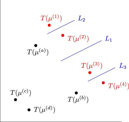
Thus, using our sequential estimation-removal method, we can identify ${\mu }^{\left(a\right)},\dots ,{\mu }^{\left(d\right)}$ (or ${\mu }^{\left(1\right)},\dots ,{\mu }^{\left(4\right)})$ by one straight line twice. However, three straight lines are required to distinguish between $\left\{T\right({\mu }^{\left(1\right)}),T({\mu }^{\left(3\right)}\left)\right\}$ and $\left\{T\right({\mu }^{\left(2\right)}),$ $T\left({\mu }^{\left(4\right)}\right)\}$ (e.g. $L_1,$ $L_2,$ and $L_3$). Therefore, only one straight line is required to distinguish between ${\mu }^{\left(a\right)}$ and ${\mu }^{\left(b\right)},$ but three straight lines are required to distinguish between ${\mu }^{\left(c\right)}$ and ${\mu }^{\left(d\right)}$ directly from the observation values. These mean that $T\left({\mu }^{\left(c\right)}\right)$ and $T\left({\mu }^{\left(d\right)}\right)$ are ‘buried’ in $T\left({\mu }^{\left(a\right)}\right)$ and $T\left({\mu }^{\left(b\right)}\right).$

4. Some numerical analysis of our discretized magnetic inverse problem

4.1. ‘Practical’ rank of matrix G

We consider the rank of matrix G. As described below, a ‘practical’ rank of G is significantly low. Since the fractional value of (4(4) $g_{kj}:=G(o_k-p_j).$(4) ) for given $(o_k,p_j)$ is usually not divisible and all components of G will be different from one another, the ‘exact’ rank of G probably will be full. However, in practice, two almost parallel row (or column) vectors should be considered to be exactly parallel. Thus we examine how parallel the row vectors of G are by applying the following procedure. (The modified Gram-Schmidt algorithm was used in implementing this procedure.)

Procedure 4.1

Let $g_k$ $(k=1,2,\dots ,n_o)$ denote the k-th normalized row vector of G. (If ${\overline{g}}_k$ is the kth row vector of G, then $g_k={\overline{g}}_k/\parallel {\overline{g}}_k\parallel ,$ where $\parallel \cdot \parallel$ denotes the Euclidean norm in ${\mathbb{R}}^{n_{\rho }}.$)

1.	1. Let $ϵ>0$ be a sufficiently small real number. Set $n=1.$ Let $L_1$ be the linear space spanned by $g_1$ and $u_1:=g_1.$
2.	2. Using the basis $\{u_1,\dots ,u_n\}$ of $L_n,$ calculate $u_r:=g_r-\sum _{k=1}^n\left(g_r\text{{ }\bullet \text{}}{v}_k\right)v_k,$for $r=n+1,\dots ,n_o,$ where $\$\bullet \$$ denotes the inner product.
3.	3. Calculate $h:=\underset{r=n+1,\dots ,n_o}{argmax}\parallel u_r\parallel .$Then, swap $u_{n+1}$ and $u_h,$ and swap $g_{n+1}$ and $g_h.$
4.	4. If $\parallel u_{n+1}\parallel >ϵ,$ let $L_{n+1}$ be the linear space spanned by $\{u_1,\dots ,u_n,u_{n+1}\}.$ If $\parallel u_{n+1}\parallel \le ϵ,$ stop the procedure and output $\{u_1,\dots ,u_n\}.$
5.	If $n+1=n_o,$ stop the procedure and output $\{u_1,\dots ,u_{n_o}\}.$ If $n+1<n_o,$ set $n\leftarrow n+1$ and go back to step 2.

Remark 4.2

The distribution of $\{\parallel u_n\parallel \}$ given by Procedure 4.1 depends on the order of $g_k$ specified by k. Step 2 determines this order except the selection of $g_1.$

In our numerical experiments, we set $ϵ=0.0001$ and recorded the values of $\{\parallel u_n\parallel \}$ ($\left\{u_n\right\}$ is the output). These values represent a ‘practical’ rank of G. In fact, if the value of $\parallel u_n\parallel$ is below a certain threshold (for example 0.01), we consider that $g_n$ belongs to the linear space spanned by $g_1,\dots ,g_{n-1}$ in our numerical calculations. Some results of experiments using this procedure are presented in Tables 1–4.

Table 1. ‘Practical’ rank of G (observation points: $20\times 20\times 1$).

	Charges
Length $\parallel u_n\parallel$	$20\times 20\times 10$	$20\times 20\times 6$	$20\times 20\times 1$
$\parallel u_n\parallel \ge 0.9$	400	21	9
$0.1\le \parallel u_n\parallel <0.9$	0	71	19
$0.01\le \parallel u_n\parallel <0.1$	0	94	29

Table 2. ‘Practical’ rank of G (Observation points: $20\times 20\times 4$).

	Charges
Length $\parallel u_n\parallel$	$20\times 20\times 10$	$20\times 20\times 6$	$20\times 20\times 1$
$\parallel u_n\parallel \ge 0.9$	399	22	8
$0.1\le \parallel u_n\parallel <0.9$	66	76	22
$0.01\le \parallel u_n\parallel <0.1$	214	99	29

Table 3. ‘Practical’ rank of G (observation points: $40\times 40\times 1$).

	Charges
Length $\parallel u_n\parallel$	$20\times 20\times 10$	$20\times 20\times 6$	$20\times 20\times 1$
$\parallel u_n\parallel \ge 0.9$	355	22	9
$0.1\le \parallel u_n\parallel <0.9$	45	79	22
$0.01\le \parallel u_n\parallel <0.1$	370	93	27

Table 4. ‘Practical’ rank of G (Observation points: $40\times 40\times 2$).

	Charges
Length $\parallel u_n\parallel$	$20\times 20\times 10$	$20\times 20\times 6$	$20\times 20\times 1$
$\parallel u_n\parallel \ge 0.9$	352	22	8
$0.1\le \parallel u_n\parallel <0.9$	65	78	24
$0.01\le \parallel u_n\parallel <0.1$	359	103	27

In these tables, ‘charge: $20\times 20\times h$’ means that $n_{\rho }$ $(n_{\rho }=20\times 20\times h)$ magnetic charge points $p_1,p_2,\dots ,p_{n_{\rho }}$ are arranged as follows: 20 points in the x direction at intervals of 1, 20 points in the y direction at intervals of 1 and h points in the z direction at intervals of 1. Furthermore, ‘observation points: $w_1\times w_2\times h$’ has almost the same meaning. However, when $w_1=w_2=40,$ the interval in the x direction and that in the y direction are 0.5. In Tables 1–4, the distances between the top plane of charge points and the bottom plane of observation points are 1, 5 and 10 when the number of charges is $20\times 20\times 10,$ $20\times 20\times 6$ and $20\times 20\times 1,$ respectively. For example, the first row of Table 1 means that the numbers of vectors $u_n$ with $\parallel u_n\parallel \ge 0.9$ are 400, 21 and 9 in the cases of $20\times 20\times 10,$ $20\times 20\times 6$ and $20\times 20\times 1,$ respectively.

These experimental results illustrate that a ‘practical’ rank of G is significantly low. In the case of Tables 1–4, the numbers of observation points (the numbers of row vectors) are 400 $(=n_x{n}_y),$ 1600, 1600 and 3200, respectively. When the height h of M is 6 or less, that is, when the number of charges of M is $20\times 20\times 6$ or less, the ‘practical’ rank of G is almost the same irrespective of whether the number of observation points is 400, 1600 or 3200 (cf. [3]). Moreover, based on the results of our experiments described in Section 5.3, even if the number of observation points was $n_x{n}_y,$ the estimations were almost accurate up to the 5th piece. Therefore, it is hypothesized that having over 400 observation points is not considerably advantageous when using our sequential estimation-removal method. Our inverse problem is analogous to looking into the sea and identifying objects in it. The increase in the number of observation points does not considerably increase the amount of information. It is more difficult to identify objects that are at deeper positions (see Section 4.2).

4.2. Stability/instability

We discuss the stability/instability of our discretized inverse problem (6(6) $GR\mu =f.$(6) ). Some results of our numerical experiments on the distribution of $r^{\left(\alpha \text{β}\right)}$ defined by (16(16) $\begin{array}{rl}{r}^{\left(\alpha \text{β}\right)}& :=\frac{{∥T\left({\mu }^{\left(\alpha \right)}\right)-T\left({\mu }^{\left(\text{β}\right)}\right)∥}_O}{{∥{\mu }^{\left(\alpha \right)}-{\mu }^{\left(\text{β}\right)}∥}_M}(\alpha \ne \text{β}),\\ r^{min}& :=min\left\{r^{\left(\alpha \text{β}\right)}:{\mu }^{\left(\alpha \right)},{\mu }^{\left(\text{β}\right)}\in \mathcal{M},\alpha \ne \text{β}\right\}.\end{array}$(16) ) for T = GR are shown in Figure 6. In each histogram of Figure 6, the horizontal and vertical axes represent the ratio $r^{\left(\alpha \text{β}\right)}$ and its frequency, respectively. As the value of $r^{\left(\alpha \text{β}\right)}$ decreases, the difficulty of distinction between ${\mu }^{\left(\alpha \right)}$ and ${\mu }^{\left(\alpha \right)}$ increases. If and only if $r^{\left(\alpha \text{β}\right)}>0,$ we can distinguish between ${\mu }^{\left(\alpha \right)}$ and ${\mu }^{\left(\alpha \right)}.$

Figure 6. Distributions of $r^{\left(\alpha \text{β}\right)}$

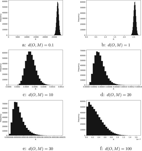
As shown in Figure 2, all the observation points are placed on the same horizontal plane in these experiments, and the number of observation points is equal to the number of cells in the horizontal direction, that is, $n_o=n_x{n}_y.$ The values of the parameters utilized are $n_x=n_y=20,$ $n_z=5$ and $n_o=n_x{n}_y=400.$ Let $d(O,M)$ denote the distance between the horizontal plane O, where the observation points are placed, and the top surface of the magnetic sample M. In Figure 6, the values of $d(O,M)$ of Figures 6(a), 6(b), …, and 6(f) are 0.1, 1, 10, 20, 30 and 100, respectively. Note that the length of each side of every cubic cell is normalized to 1. Since the number of elements of $\mathcal{M},$ $2^{n_{\mu }}=2^{2000},$ is very large, we did not conduct experiments on all pairs $\left\{\right(\alpha ,\text{β}\left)\right\},$ but on randomly selected pairs. To provide details, we randomly selected 1000 magnetic moment vectors, and we calculated $r^{\left(\alpha \text{β}\right)}$ for all (499,500 possible) pairs of these moment vectors, where the randomness means the following: the probability that the moment of each cell is 1 and the probability that it is $-1$ are both 0.5.

Let decompose ${\mu }^{\left(\alpha \right)}$ and ${\mu }^{\left(\text{β}\right)}$ such that ${\mu }^{\left(\alpha \right)}={\mu }_U^{\left(\alpha \right)}+{\mu }_L^{\left(\alpha \right)},{\mu }^{\left(\text{β}\right)}={\mu }_U^{\left(\text{β}\right)}+{\mu }_L^{\left(\text{β}\right)},$where $(\cdot {)}_U$ is an upper part and $(\cdot {)}_L$ is a lower part. Assume ${\mu }_U^{\left(\alpha \right)}={\mu }_U^{\left(\text{β}\right)},$ then (26) $r^{\left(\alpha \text{β}\right)}=\frac{{∥T\left({\mu }^{\left(\alpha \right)}\right)-T\left({\mu }^{\left(\text{β}\right)}\right)∥}_O}{{∥{\mu }^{\left(\alpha \right)}-{\mu }^{\left(\text{β}\right)}∥}_M}=\frac{{∥T\left({\mu }_L^{\left(\alpha \right)}\right)-T\left({\mu }_L^{\left(\text{β}\right)}\right)∥}_O}{{∥{\mu }_L^{\left(\alpha \right)}-{\mu }_L^{\left(\text{β}\right)}∥}_M}.$(26) In such a case, we can also consider that $d(O,M)$ in Figure 6 is the sum of the depth of the upper pieces and the distance between the horizontal plane O and the top surface of the magnetic sample M. Therefore, for example, we can consider that when we can estimate nine pieces from the top correctly, the histogram of Figure 6(c) represents the difficulty of estimating the pieces below them.

Thus the experimental results numerically illustrate that the magnetic moment distribution to a certain depth can be estimated from the MFM images, and the estimation becomes difficult as the depth increases. This property is independent of the choice of reconstruction method. One of the reasons for this difficulty is explained below. We consider two cells $c_j$ and $c_{j+1}$ that are horizontally adjacent, and the ratio of distances from $p_j$ and $p_{j+1}$ (the centre points of the top faces of $c_j$ and $c_{j+1}$) to observation point $o_k,$ i.e. $\parallel p_{j+1}-o_k\parallel /\parallel p_j-o_k\parallel .$ As points $p_j$ and $p_{j+1}$ become farther away from point $o_k,$ this ratio becomes closer to 1; consequently, the ratio $g_{k,j+1}/g_{kj}$ also becomes closer to 1, where $g_{kj}$ is the kj-component of G. Thus, using the observed value at point $o_k,$ it becomes difficult to distinguish between the case of $({\mu }_j,{\mu }_{j+1})=(1,-1)$ and that of $({\mu }_j,{\mu }_{j+1})=(-1,1).$

The above-mentioned experimental results on the distribution of $r^{\left(\alpha \text{β}\right)}$ are for a given discretization. Making the cell discretization finer is the same as reducing the size (the length of each side) of each cell. Let the size of cells, the interval between every pair of observation points, and the value of $d(O,M)$ be smaller at the same ratio; we denote this ratio by s. Then, the shape of the histogram of the distribution of $\left\{r^{\left(\alpha \text{β}\right)}\right\}$ does not change. Therefore, the shape of the histogram when the size of cells and the interval between the observation points are both multiplied by s without changing $d(O,M)$ is the same as that of the histogram when only $d(O,M)$ is multiplied by $1/s.$ For example, we can consider the histogram f of Figure 6 to be the histogram for the case where $d(O,M)=1,$ the size of cells is $1/100,$ and the interval between the observation points is $1/100.$ This case is the 1/100 subdivision of the case b of Figure 6 (for a magnet sample with $1/{100}^3$ size). Similarly, we can consider cases c, d and e in Figure 6 to be the $1/10,$ 1/20 and 1/30 subdivisions of case b, respectively. Thus we have the following experimental claim.

Experimental claim 4.3

The inverse problem (6(6) $GR\mu =f.$(6) ) is unstable for cell subdivision. Therefore, assumption (vi) in Section 2.2 should hold with sufficient accuracy for some cell discretization. In other words, only such magnets can be considered.

This claim is compatible with the property that the solution ρ of integral Equation (2(2) $F_z^{\prime }\left(r\right)=\left(\mathcal{G}\rho \right)\left(r\right):={\int }_{M}G(r-r^{\prime })\rho \left(r^{\prime }\right)d{r}^{\prime },$(2) ) is generally not unique for given data $F_z^{\prime }.$

Procedure 3.4 needs Assumption 3.5, and from Lemma 3.8, Assumption 3.5 is related to $r_{\left[\ell \right]\downarrow }^{\left(\alpha \text{β}\right)}$ defined by (21(21) $r_{\left[\ell \right]\downarrow }^{\left(\alpha \text{β}\right)}:=\frac{{∥T\left({\mu }_{\left[\ell \right]\downarrow }^{\left(\alpha \right)}\right)-T\left({\mu }_{\left[\ell \right]\downarrow }^{\left(\text{β}\right)}\right)∥}_O}{{∥{\mu }_{\left[\ell \right]}^{\left(\alpha \right)}-{\mu }_{\left[\ell \right]}^{\left(\text{β}\right)}∥}_M}(\alpha \ne \text{β})$(21) ) and $r_{\left[\ell \right]}$ defined by (22(22) $r_{\left[\ell \right]}:=min\left\{r_{\left[\ell \right]\downarrow }^{\left(\alpha \text{β}\right)}:{\mu }_{\left[\ell \right]}^{\left(\alpha \right)},{\mu }_{\left[\ell \right]}^{\left(\text{β}\right)}\in {\mathcal{M}}_{\left[\ell \right]},\alpha \ne \text{β}\right\}.$(22) ). If $L=\left[\ell \right]\downarrow$ in (26(26) $r^{\left(\alpha \text{β}\right)}=\frac{{∥T\left({\mu }^{\left(\alpha \right)}\right)-T\left({\mu }^{\left(\text{β}\right)}\right)∥}_O}{{∥{\mu }^{\left(\alpha \right)}-{\mu }^{\left(\text{β}\right)}∥}_M}=\frac{{∥T\left({\mu }_L^{\left(\alpha \right)}\right)-T\left({\mu }_L^{\left(\text{β}\right)}\right)∥}_O}{{∥{\mu }_L^{\left(\alpha \right)}-{\mu }_L^{\left(\text{β}\right)}∥}_M}.$(26) ), we have $r^{\left(\alpha \text{β}\right)}\le r_{\left[\ell \right]\downarrow }^{\left(\alpha \text{β}\right)}.$ Some further experimental consideration for $r_{\left[\ell \right]\downarrow }^{\left(\alpha \text{β}\right)}$ is described in Section 4.3.

4.3. Properties of the pieces of $\mathcal{M}$ defined in Section 2.3

We consider some properties of the pieces $\left\{{\mathcal{M}}_{\left[\ell \right]}\right\}$ of $\mathcal{M}$ defined in Section 2.3 for the case where $n_x=n_y=20$ (Tables 5, 7 and 9) or $n_x=n_y=32$ (Tables 6, 8 and 10), $\overline{m}=n_z=10,$ $n_o=n_x{n}_y$ and $d(O,M)=1.$ We numerically calculated the minimum and average of $\left\{r_{\left[\ell \right]\downarrow }^{\left(\alpha \text{β}\right)}\right\}$ (defined by (21(21) $r_{\left[\ell \right]\downarrow }^{\left(\alpha \text{β}\right)}:=\frac{{∥T\left({\mu }_{\left[\ell \right]\downarrow }^{\left(\alpha \right)}\right)-T\left({\mu }_{\left[\ell \right]\downarrow }^{\left(\text{β}\right)}\right)∥}_O}{{∥{\mu }_{\left[\ell \right]}^{\left(\alpha \right)}-{\mu }_{\left[\ell \right]}^{\left(\text{β}\right)}∥}_M}(\alpha \ne \text{β})$(21) )), the minimum and maximum of $\{\parallel GR{\mu }_{\left[\ell \right]}\parallel \},$ and the minimum and average of $\{\parallel GR{\mu }_{\left[\ell \right]}{\parallel }_O/\parallel GR{\mu }_{[\ell +1]}{\parallel }_O\},$ where ${\mu }_{\left[\ell \right]}={\mu }_{[\ell +1]}$ as $n_x{n}_y$-dimensional vectors.

Table 5. Minimum and average of $\{1000\cdot r_{\left[\ell \right]\downarrow }^{\left(\alpha \text{β}\right)}\}$ $(n_x=n_y=20)$.

Piece ℓ	1	2	3	4	5	6	7	8	9	10
Minimum	4832	271	59.6	18.0	7.12	3.57	1.78	0.943	0.459	0.256
Average	5715	347	82.6	30.4	13.9	7.27	4.12	2.46	1.48	0.827

Table 6. Minimum and average of $\{1000\cdot r_{\left[\ell \right]\downarrow }^{\left(\alpha \text{β}\right)}\}$ $(n_x=n_y=32)$.

Piece ℓ	1	2	3	4	5	6	7	8	9	10
Minimum	5076	303	67.9	22.8	9.97	4.58	2.52	1.43	0.835	0.437
Average	5715	348	83.7	30.9	14.2	7.44	4.27	2.58	1.56	0.864

Table 7. Minimum and maximum of $\{1000\cdot \parallel GR{\mu }_{\left[\ell \right]}{\parallel }_O\}$ $(n_x=n_y=20).$

Piece ℓ	1	2	3	4	5	6	7	8	9	10
Minimum	117,000	7550	1860	695	304	150	79.9	48.2	32.3	22.5
Maximum	124,000	10,100	3220	1440	799	495	337	239	175	131

Table 8. Minimum and maximum of $\{1000\cdot \parallel GR{\mu }_{\left[\ell \right]}{\parallel }_O\}$ $(n_x=n_y=32).$

Piece ℓ	1	2	3	4	5	6	7	8	9	10
Minimum	189,000	12,900	3370	1320	620	333	183	109	70.6	49.0
Maximum	197,000	15,400	4830	2120	1140	702	460	314	222	170

Table 9. Minimum and average of $\{\parallel GR{\mu }_{\left[\ell \right]}{\parallel }_O/\parallel GR{\mu }_{[\ell +1]}{\parallel }_O:{\mu }_{\left[\ell \right]}={\mu }_{[\ell +1]}\}$ $(n_x=n_y=20)$.

Pieces pair $(\ell ,\ell +1)$	(1,2)	(2,3)	(3,4)	(4,5)	(5,6)	(6,7)	(7,8)	(8,9)	(9,10)
Minimum	11.7	3.00	2.02	1.70	1.50	1.39	1.32	1.27	1.23
Average	13.8	3.57	2.42	1.99	1.76	1.62	1.52	1.45	1.40

Table 10. Minimum and average of $\{\parallel GR{\mu }_{\left[\ell \right]}{\parallel }_O/\parallel GR{\mu }_{[\ell +1]}{\parallel }_O:{\mu }_{\left[\ell \right]}={\mu }_{[\ell +1]}\}$ $(n_x=n_y=32)$.

Pieces pair $(\ell ,\ell +1)$	(1,2)	(2,3)	(3,4)	(4,5)	(5,6)	(6,7)	(7,8)	(8,9)	(9,10)
Minimum	12.4	3.12	2.13	1.77	1.52	1.42	1.36	1.31	1.26
Average	13.7	3.54	2.40	1.97	1.75	1.61	1.51	1.44	1.39

First, for each ℓ $(\ell =1,2,\dots ,10),$ we randomly selected 1000 magnetic moment vectors, and we calculated $r_{\left[\ell \right]\downarrow }^{\left(\alpha \text{β}\right)}$ for all (499,500 possible) pairs of those moment vectors as in the case of Figure 6. The experimental results of the minimum and average of $\left\{r_{\left[\ell \right]\downarrow }^{\left(\alpha \text{β}\right)}\right\}$ are shown in Tables 5 and 6, where the values are multiplied by 1000 and the fourth digit from the top of each value is rounded off. In the cases of this section, the results of Tables 5 and 6 numerically imply $r_{\left[1\right]}>r_{\left[2\right]}>\cdots >r_{\left[10\right]}>0,$ where $r_{\left[\ell \right]}=min\left\{r_{\left[\ell \right]\downarrow }^{\left(\alpha \text{β}\right)}\right\}.$ Therefore, from Lemma 3.8 (i) and (22(22) $r_{\left[\ell \right]}:=min\left\{r_{\left[\ell \right]\downarrow }^{\left(\alpha \text{β}\right)}:{\mu }_{\left[\ell \right]}^{\left(\alpha \right)},{\mu }_{\left[\ell \right]}^{\left(\text{β}\right)}\in {\mathcal{M}}_{\left[\ell \right]},\alpha \ne \text{β}\right\}.$(22) ), there exist $T_{\left[\ell \right]}^{-1}$ $(\ell =1,\dots ,10)$ of Assumption 3.5 (i) and inequalities (24(24) $r_{\left[1\right]}\ge r_{\left[2\right]}\ge \cdots \ge r_{\left[\overline{m}\right]}\left(\text{if possible, }{r}_{\left[1\right]}>r_{\left[2\right]}>\cdots >r_{\left[\overline{m}\right]}\right)$(24) ) satisfy for $\ell =1,\dots ,10.$ However, if the true value of $r_{\left[\ell \right]}$ is smaller than the calculation error, then $T_{\left[\ell \right]}^{-1}$ may not be obtained by any method.

Next, for each ℓ $(\ell =1,2,\dots ,10),$ we randomly selected 10,000 magnetic moment vectors, and we calculated the minimum and maximum of $\{\parallel GR{\mu }_{\left[\ell \right]}{\parallel }_O\}.$ The experimental results are shown in Tables 7 and 8, where the values are multiplied by 1000 and the fourth digit from the top of each value is rounded off. Tables 7 and 8 numerically illustrate that piece monotonicity holds for $(\ell ,\ell +1)=(1,2),(2,3),(3,4)$ when $n_x=n_y=20$ and for $(\ell ,\ell +1)=(1,2),\dots ,(4,5)$ when $n_x=n_y=32.$

When $x=y=0,$ the Green function $G\left(r\right)$ of (3(3) $G\left(r\right)=\frac{15z^3-9z\left(x^2+y^2+z^2\right)}{{\left(x^2+y^2+z^2\right)}^{7/2}}.$(3) ) becomes $G\left(r\right)=6/z^4.$ Therefore, roughly speaking, the values in Tables 5–8 decrease proportionally to ${\ell }^{-4}.$

Next, for each ℓ $(\ell =1,2,\dots ,10),$ we randomly selected 10,000 magnetic moment vectors $\left\{\mu \right\},$ where ${\mu }_{\left[\ell \right]}={\mu }_{[\ell +1]}$ $(\ell =1,2,\dots ,9)$ as $n_x{n}_y$-dimensional vectors, and we calculated the minimum and average of $\{\parallel GR{\mu }_{\left[\ell \right]}{\parallel }_O/\parallel GR{\mu }_{[\ell +1]}{\parallel }_O\}.$ The experimental results are shown in Tables 9 and 10, where the fourth digit from the top of each value is rounded off. Tables 9 and 10 numerically illustrate that weak piece monotonicity holds for $(\ell ,\ell +1)=(1,2),\dots ,(9,10)$ in the cases considered in this subsection.

Thus, we have the following.

Experimental claim 4.4

As the value of ℓ increases, all the values in Tables 5–10 decrease. These tables show numerically that the above-mentioned selection of ${\mathcal{M}}_{\left[\ell \right]}$ approximately satisfies the properties in step 1 of Procedure 3.9. Therefore, we consider the selection is appropriate.

This will be correct if we somewhat change the values of $n_x,$ $n_y$ and $n_z.$

4.4. Conclusion of this section

Based on the experimental results of this section, it is possible that $\text{Ker }\widetilde{GR}\ne \left\{0\right\}$ and $(GR{)}^{-1}$ exist. Then, $(GR{)}^{-1}$ is not linear, and it is difficult to solve our inverse problem using a linear algebraic approach. In the following sections, we aim to estimate the magnetic moments as much as possible using our sequential estimation-removal method. In Sections 5 and 6, we utilize assumption (i)–(vii) of Section 2.2. However, the results of this section indicate that the performances of $N_{\left[\ell \right]}\approx T_{\left[\ell \right]}^{-1}$ (Section 5) and the iterative method (Section 6) decrease as ℓ increases. Furthermore, the results of our numerical experiments described in Sections 5 and 6 are compatible with that. One of the reasons is the performance limit of our personal computer (PC); however, it is impossible to estimate magnetic moments at deep positions accurately using any method. In general situations where assumptions (vi) and (vii) are not satisfied, the problem becomes even more difficult.

5. Deep learning and experimental results

To solve the discretized (nonlinear) binary inverse problem (6(6) $GR\mu =f.$(6) ), we consider two numerical methods using Procedure 3.4 with Procedure 3.9. (As described at the end of Section 3.2, we used Procedure 3.4 in the following experiments.) One method is to construct a neural network, such as $N_{\left[\ell \right]}\approx T_{\left[\ell \right]}^{-1},$ while the other method is to employ an iterative algorithm as an approximate $T_{\left[\ell \right]}^{-1}.$ We study the former method in this section and the latter method in the next section. Since f can be easily calculated for any given μ using (6(6) $GR\mu =f.$(6) ), we can obtain numerous training data. Deep learning of a neural network requires a high computational cost. However, when such a neural network is obtained, it can be applied with a lower computational cost than that of an iterative method. In this and the next sections, we use assumption (i)–(vii) provided in Section 2.2 and the following setting of experiments.

Setting 5.1 As shown in Figure 2, all the observation points are placed on the same horizontal plane, and the number of observation points is equal to the total number of cells in the horizontal direction, that is, $n_o=n_x{n}_y.$

This setting is based on the results of Section 4.1. In the following experiments, the sizes of $n_x,$ $n_y,$ $n_z,$ and data are attributed to the performance limit of our PC, especially its memory size (see Table 11).

Table 11. Execution environment.

OS	Windows 10 Home
CPU	Core i7 4.20 GHz
GPU	NVIDIA GeForceGTX 1080
Memory	16.0 GB
Language	Python 3.6.0
AI Library	TensorFlow 1.4.0, Keras 2.0.9

5.1. Structure of neural networks

Based on Setting 5.1, ‘the number of nonzero components of ${\mu }_{\left[\ell \right]}$’ $=n_x{n}_y=n_o=\dim {\mathbb{R}}^{n_o}$ for every ℓ. Therefore, in a neural network $N_{\left[\ell \right]}\approx T_{\left[\ell \right]}^{-1}:{\mathbb{R}}^{n_o}\to {\mathcal{M}}_{\left[\ell \right]},$ the number of input nodes and that of output nodes are both equal to $n_0.$ We consider our discretized inverse problem to be a type of image classification problem and construct each $N_{\left[\ell \right]}$ $(\ell =1,2,\dots ,n_z)$ using a convolutional autoencoder provided by Keras/Tensorflow (see [14]). (In our numerical experiments, we did not assume any structure for the magnetic moment configurations of the training data; however, if it had some geometrical structure, a convolutional auto encoder would be more effective. Furthermore, if we could construct a neural network suitable for such a geometrical structure, it would be even more effective.)

In our numerical experiments, we set $n_x=n_y=32,$ $n_z=10$ and $n_o=n_x{n}_y=1024.$ Then, the structure of each $N_{\left[\ell \right]}$ is shown in Figure 7. This figure was drawn by the plot_model function of the keras.utils module. In our experiments, the values of parameters are as follows:

• Size of the kernel: $3\times 3$ in all layers;

• Strides: $1\times 1$ in conv2d_4 and $2\times 2$ in the other layers;

• Padding: 0 padding in all layers;

• The number of filters, as depicted in Figure 7, that is, 256.

Figure 7. Convolutional auto encoder.

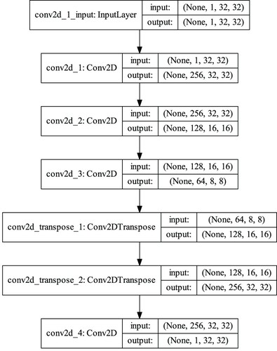
The activation function is the linear function (the identity function) in the output layer and the rectified linear function in the other layers. Each input node corresponds to the observation value at each observation point. Each output node corresponds to the magnetic moment of each cell. In the training, the loss function is the mean squared error function (25(25) ${∥N_{\left[\ell \right]}\left(T\left({\mu }_{\left[\ell \right]\downarrow }\right)\right)-{\mu }_{\left[\ell \right]}∥}_M^2.$(25) ) (see [15]). In the tests, it is considered that the value of the magnetic moment is 1 if the output value is greater than 0, and $-1$ if it is less than 0.

Remark 5.2

We consider $\left\{f_{\left[\ell \right]}\right\}$ for $\ell =1,2,\dots ,n_z,$ where $f_{\left[\ell \right]}=T\left({\mu }_{\left[\ell \right]}\right)$ and $\left\{f_{\left[\ell \right]}\right\}$ denote the set of all possible $f_{\left[\ell \right]}.$ Note that the maximum possible number of the elements of $\left\{f_{\left[\ell \right]}\right\}$ equals the number of all possible ${\mu }_{\left[\ell \right]},$ i.e. $2^{n_o}=2^{n_x{n}_y}$ for every $\ell =1,2,\dots ,n_z.$ For matrix G defined in Section 2.2, we put $G_{\left[\ell \right]\downarrow }:=\left(h_{kj}\right),$ where the size of $G_{\left[\ell \right]\downarrow }$ is the same as the size of G and $h_{kj}:=\left\{\begin{array}{lll}{g}_{kj}& & \text{if }j=a(n_z+1)+b,a=0,1,\dots ,n_x{n}_y-1,b=\ell ,\ell +1,\dots ,n_z+1\\ 0& & \text{otherwise}.\end{array}\right.$As described in Section 4.1, the ‘practical’ rank of G is smaller than $n_{\rho }=n_x{n}_y(n_z+1),$ and the ‘practical’ rank of $G_{\left[\ell \right]\downarrow }$ decreases rapidly as ℓ increases. Therefore, the ‘practical’ dimension of the space spanned by $\left\{f_{\left[\ell \right]}\right\}$ decreases as ℓ increases. In general, if $\mathcal{A}$ is a d-dimensional hyperplane arrangement that consists of m hyperplanes in general position, the number of regions of $\mathcal{A}$ is given by $\sum _{i=0}^d\left(\begin{array}{c}m\\ i\end{array}\right)$(see Proposition 2.4 of [16]). Therefore, when using hyperplanes to distinguish $\left\{f_{\left[\ell \right]}\right\},$ it is almost certain that more hyperplanes will be required as ℓ increases. In other words, the size of neural network $N_{\left[\ell \right]}$ almost certainly have to increase as ℓ increases (cf. [13]). However, we used $N_{\left[\ell \right]}$ depicted in Figure 7 for every ℓ because of the performance limit of our PC.

5.2. Deep learning

In our numerical experiments, unless otherwise noted, we set $n_x=n_y=32,$ $\overline{m}=n_z=10,$ $n_o=n_x{n}_y=1024,$ the length of each side of every cubic cell of the (discretized) magnetic sample M to 1, and $d(O,M)$ to 1. The number of elements of $\mathcal{M}$ was $2^{n_{\mu }}=2^{10240},$ and we randomly chose elements $\left\{\mu \right\}$ from $\mathcal{M}$ to make training data $\left\{\right(\mu ,GR\mu \left)\right\}.$ Such a moment vector μ can be obtained as follows.

1. Set $\mu =[{\mu }_1,{\mu }_2,\dots ,{\mu }_{n_{\mu }}{]}^t=[1,1,\dots ,1{]}^t.$

2. $i\leftarrow 1.$

3. Change ${\mu }_i$ to $-1$ with probability r. (We call r the reversal rate.)

4. $i\leftarrow i+1$ and go back to step 3.

Making a neural network is more difficult, as the problem is more complex. Therefore, in our numerical experiment, we set r to be a fixed constant instead of a variable. Then, neural networks with several reversal rates may be used to estimate magnetization, and the estimation result closest to the observed data may be adopted. (In the actual experiments, we can apply a vibrating-sample magnetometer (VSM) to measure the magnitude of the overall magnetic moment of the sample, that is, to measure the reversal rate.) We consider the simple and fundamental case where it is randomly determined which cell moments are reversed. (In the ideal high-performance magnet, the orientation of the moments of the magnetic grains are approximately independent of each other.) Therefore, in our numerical experiment, we made the reversal rate common to all μ. Its value was 0.1, 0.3 or 0.5 (we considered these three cases); we made training data comprising 8000 pairs for each reversal rate. In deep learning, we employed Adam to update weights, where the values of the parameters of Adam were the default values given in [17] (cf. [18]).

In the noiseless cases, we expected $\overline{\overline{m}}=\overline{m}=n_z$ based on the experimental analysis in Section 4 (see Remark 5.3). Let $N^s:=(N_{\left[1\right]}^s,N_{\left[2\right]}^s,\dots ,N_{\left[n_z\right]}^s)$ be the obtained neural network by using the training data of reversal rate s, where $s=0.1,0.3,$ and $\mathrm{0.5.}$ In our experiments, to examine the performances of these neural networks, we randomly generated a set of test data $\left\{\right(\mu ,GR\mu \left)\right\}$ consisting of 2000 pairs with fixed reversal rates r = 0.1, 0.2, 0.3, 0.4 and $\mathrm{0.5.}$

Let $\mathcal{R}$ be a set of some reversal rates (in our experiments, $\mathcal{R}=\{0.1,0.3,0.5\}$) and assume that we made $N^s$ $(s\in \mathcal{R}).$ When an observation values vector f is given, we calculate ${\mathcal{E}}_f\left(s\right):=\sum _{\ell =1}^{n_z}{∥f-\sum _{k=1}^{\ell }GR\left(N_{\left[k\right]}^s\left(f\right)\right)∥}^2(s\in \mathcal{R}),$and put $r_f^{\ast }:=\underset{s\in \mathcal{R}}{\text{argmin}}{\mathcal{E}}_f\left(s\right).$Then, we consider that $N^{r_f^{\ast }}$ is the most appropriate neural network in $\{N^s:s\in \mathcal{R}\}$ for estimating μ such that $GR\mu (+\delta )=f$ for the given f.

The execution environment of our experiments is presented in Table 11.

5.3. Experimental results of the noiseless cases

The relationship between the theoretical consideration in Section 3, the experimental analysis in Section 4, and the following experimental results is described in Remark 5.3.

For the generated noiseless test data $\left\{\right(\mu ,f\left)\right\}=\left\{\right(\mu ,GR\mu \left)\right\}$ with the reversal rates $r=0.1,0.2,0.3,0.4$ and $0.5,$ the rates defined by $r^{\ast }:=\underset{s\in \{0.1,0.3,0.5\}}{\text{argmin}}\sum _f{\mathcal{E}}_f\left(s\right)$are summarized in Table 12, respectively.

Table 12. Reversal rates.

r (rate of data)	0.1	0.2	0.3	0.4	0.5
$r^{\ast }$	0.1	0.3	0.3	0.5	0.5

The estimation performances of $N^s$ $(s=0.1,0.3,$ and $0.5)$ are presented in Table 13. There were $32\times 32$ cells in each piece, and the set of test data $\left\{\right(\mu ,GR\mu \left)\right\}$ consisted of 2000 pairs. Therefore, $32\times 32\times 2000=2,048,000$ magnetic moments should be estimated. In Table 13, rate r is the reversal rate of the test data and rate s is the reversal rate of $N^s.$ ${0.1}^{\ast },$ ${0.3}^{\ast },$ and ${0.5}^{\ast }$ means that s is $r^{\ast }$ of Table 12. The values in Table 13 illustrate what percentage of these 2,048,000 moments were correctly estimated. These values are rounded off to three decimal places. Therefore, 1.000 means a value of 0.9995 or more. Table 13 shows that, up to the 5th piece, the estimations were almost accurate if $s=r^{\ast }.$

Table 13. Estimation performances of each rate.

Rates		Piece
r	s	1	2	3	4	5	6	7	8	9	10
0.1	${0.1}^{\ast }$	1.000	1.000	1.000	1.000	0.996	0.964	0.866	0.773	0.731	0.772
0.1	0.3	1.000	1.000	1.000	0.997	0.971	0.831	0.654	0.614	0.612	0.654
0.1	0.5	1.000	0.978	0.861	0.652	0.511	0.487	0.524	0.505	0.541	0.487
0.2	0.1	1.000	1.000	1.000	0.991	0.923	0.752	0.683	0.673	0.640	0.704
0.2	${0.3}^{\ast }$	1.000	1.000	1.000	0.999	0.978	0.826	0.621	0.583	0.578	0.601
0.2	0.5	1.000	0.997	0.978	0.868	0.636	0.514	0.518	0.505	0.530	0.492
0.3	0.1	1.000	1.000	0.993	0.922	0.715	0.612	0.609	0.595	0.592	0.627
0.3	${0.3}^{\ast }$	1.000	1.000	1.000	0.999	0.975	0.788	0.580	0.554	0.553	0.563
0.3	0.5	1.000	1.000	0.998	0.979	0.834	0.569	0.514	0.505	0.517	0.494
0.4	0.1	1.000	0.995	0.942	0.721	0.571	0.538	0.536	0.533	0.545	0.558
0.4	0.3	1.000	1.000	1.000	0.991	0.909	0.644	0.537	0.528	0.529	0.532
0.4	${0.5}^{\ast }$	1.000	1.000	1.000	0.997	0.938	0.663	0.515	0.505	0.508	0.497
0.5	0.1	1.000	0.972	0.787	0.537	0.501	0.501	0.500	0.500	0.500	0.500
0.5	0.3	1.000	0.999	0.991	0.927	0.706	0.518	0.502	0.501	0.500	0.500
0.5	${0.5}^{\ast }$	1.000	1.000	1.000	0.999	0.968	0.721	0.517	0.503	0.501	0.501

Further, we conducted experiments in the cases of $d(O,M)=0.1,0.2,\dots ,$ and $\mathrm{0.9.}$ The experimental results when $r=r^{\ast }=0.5$ are illustrated in Table 14. In the cases of $d(O,M)=0.1,0.2,0.3,$ and $0.4,$ the training of $N_{\left[1\right]}=N_{\left[1\right]}^{0.5}$ did not perform well. We consider the reason is as follows. Let $o_k=(x_k,y_k,z_k)$ $(k=1,2,\dots ,n_o=1024)$ be the observation points and $p_j=(x_j^{\prime },y_j^{\prime },z_j^{\prime })$ $(j=1,2,\dots ,n_o=1024)$ be the magnet charge points on the top surface of the magnet sample described in Section 2.2. If $x_k=x_j^{\prime }$ and $y_k=y_j^{\prime },$ then $d(O,M)=z_k-z_j^{\prime }.$ In this case, we have $G(o_k-p_j)=6/(z_k-z_j^{\prime }{)}^4.$ Therefore, if $d(O,M)$ is too small, the numerical calculation for estimating the top peace will be unstable. Consequently, in the cases of $d(O,M)=0.1,0.2,0.3,$ and $0.4,$ the performance of $N_{\left[1\right]}$ will be considerably poor. The estimation of the top piece fails, then the estimation of the second piece and below also fails. In such a case, it may be appropriate to change the unit of length.

Table 14. Estimation performances of each $d(O,M)$.

	Piece
$d(O,M)$	1	2	3	4	5	6	7	8	9	10
0.1	0.500	0.500	0.500	0.500	0.499	0.500	0.500	0.499	0.500	0.500
0.4	0.500	0.502	0.500	0.500	0.500	0.499	0.500	0.500	0.500	0.499
0.5	1.000	1.000	1.000	0.999	0.994	0.880	0.570	0.506	0.501	0.500
0.6	1.000	0.999	0.999	0.999	0.990	0.844	0.548	0.506	0.501	0.501
0.9	1.000	0.999	0.999	0.999	0.975	0.755	0.522	0.503	0.501	0.501
1.0	1.000	1.000	1.000	0.999	0.968	0.721	0.517	0.503	0.501	0.501

In the case of $d(O,M)=0.5,$ the estimation performance was the highest, and the estimation performance decreased as the value of $d(O,M)$ increased. However, even if $d(O,M)=0.5,$ the estimation performance of the pieces below the 6th piece was low.

As described in Section 4.2, it is more difficult to estimate magnetic moments at deeper positions. To estimate such difficult-to-identify moments, a sufficiently large neural network and enough training data will be required. Owing to the limitations of our execution environment, we cannot enlarge the neural networks or increase the training data beyond in the above-mentioned experiments. However, in connection with this, we conducted the following experiment: the case of $n_x=n_y=20,$ $n_z=10,$ $n_o=n_x{n}_y,$ $d(O,M)=1,$ and the number of filters $N_f$ were 256 or 512. In the case of $N_f=512,$ the degree of freedom of the neural network is higher than that of the above-mentioned experiments. Both the reversal rates of the training data (8000 pairs) and the test data (2000 pairs) were 0.5. In this case, since the size of the neural networks is smaller than that in the above-mentioned experiments, we can consider that there are relatively more data. The experimental results are presented in Table 15. The experimental results of the $32\times 32$ case are also listed again for reference, and these three results are similar. As described in Remarks 5.2 and 5.3, a larger neural network may be required as magnetic charges are at deeper positions.

Table 15. Estimation performance for the size of the problem and the number of filters.

	Piece
size & $N_f$	1	2	3	4	5	6	7	8	9	10
$20\times 20,$ 256	1.000	1.000	1.000	0.998	0.961	0.710	0.517	0.503	0.501	0.500
$20\times 20,$ 512	1.000	1.000	1.000	0.998	0.964	0.727	0.524	0.505	0.503	0.501
$32\times 32,$ 256	1.000	1.000	1.000	0.999	0.968	0.721	0.517	0.503	0.501	0.501

In our sequential estimation-removal method, the errors of the estimates that are made at the upper pieces are transmitted to the lower pieces. Thus the neural networks $N_{\left[\ell \right]}$ for the lower pieces cannot perform well. This is unavoidable, but if no error occurs in the upper pieces, then the estimation results by using $N_{\left[\ell \right]}$ are better. In the case of $n_x=n_y=32,$ $n_z=10,$ $n_o=n_x{n}_y,$ and $d(O,M)=1,$ the estimation performance of $N_{\left[\ell \right]}^r$ is shown in Table 16 based on the assumption that no error occurred in the upper pieces. In these experiments, the reversal rates were common to the training data and test data $(r=r^{\ast }=0.1,0.3,0.5).$

Table 16. Estimation performance when no error occurs in the upper pieces.

	Piece
Rate	1	2	3	4	5	6	7	8	9	10
0.1	1.000	1.000	1.000	1.000	0.998	0.986	0.952	0.921	0.907	0.906
0.3	1.000	1.000	1.000	0.999	0.986	0.903	0.829	0.781	0.754	0.749
0.5	1.000	1.000	1.000	0.999	0.981	0.882	0.795	0.738	0.704	0.693

Remark 5.3

According to the experimental results in Tables 5 and 6 in Section 4.3, it is expected that $r_{\left[\ell \right]\downarrow }^{\left(\alpha \text{β}\right)}>0$ holds for all possible pairs $(\alpha ,\text{β})$ and $\ell =1,\dots ,10.$ We assume this is true; then, it is theoretically possible to estimate up to the piece of $\ell =10.$ However, the performance of the neural networks in our experiment are insufficient to estimate the pieces after $\ell =6.$ It is known that an arbitrary function can be approximated with an arbitrary accuracy using a sufficiently large neural network. Therefore, if sufficiently large neural networks are used, it is expected to be able to estimate the pieces of $\ell =6,\dots ,10.$ However, the authors do not know how large neural networks should be used. Furthermore, even if the minimum value $r_{\left[\ell \right]}$ is positive, $T_{\left[\ell \right]}^{-1}$ may not be obtained if $r_{\left[\ell \right]}$ is smaller than the calculation error.

5.4. Experimental results on cases with noise

In this section, $n_x=n_y=32,$ $n_z=10,$ $n_o=n_x{n}_y=1024,$ $d(O,M)=1,$ $r=0.5,$ and $N_f=256.$ We used neural networks of $r^{\ast }=\mathrm{0.5.}$ Table 17 presents the experimental results for cases where the data contain noise. The description of the experimental results for 6–10 pieces are omitted. Let $f=(f_1,\dots ,f_{n_o})$ be a noiseless observation values vector, $f=GR\mu ,$ and set $\overline{f}:=\sum _{i=1}^{n_o}|f_i|/n_o.$ Let $u_i$ denote a uniform random number in the interval $[-0.5,0.5].$ Then, in Table 17, the noised value ${\tilde{f}}_i$ was made by ${\tilde{f}}_i=f_i+\nu \overline{f}{u}_i,$where $\nu =0.001$ and $\mathrm{0.01.}$ (The actual MFM measurement error is typically estimated to be within 1 %.) As can be seen from this table, the estimation is extremely difficult when there is noise. We discuss how to avoid this difficulty somewhat in this section and Section 7.

Table 17. Estimation performance for cases with noise.

	Piece
Noise	1	2	3	4	5
0	1.000	1.000	1.000	0.999	0.968
0.001	1.000	1.000	0.993	0.545	0.504
0.01	1.000	1.000	0.618	0.506	0.500

We roughly estimate the size of $\eta \in {\mathrm{\Delta }}_{\left[\ell \right]\downarrow },$ which satisfies inequality (23(23) $\frac{2}{r_{\left[\ell \right]}}\underset{\eta \in {\mathrm{\Delta }}_{\left[\ell \right]\downarrow }}{sup}{∥\eta ∥}_O<{∥{\mu }_{\left[\ell \right]}^{\left(\alpha \right)}-{\mu }_{\left[\ell \right]}^{\left(\text{β}\right)}∥}_M.$(23) ). When ${\mu }_{\left[\ell \right]}^{\left(\alpha \right)}\ne {\mu }_{\left[\ell \right]}^{\left(\text{β}\right)},$ the right-hand side of (23(23) $\frac{2}{r_{\left[\ell \right]}}\underset{\eta \in {\mathrm{\Delta }}_{\left[\ell \right]\downarrow }}{sup}{∥\eta ∥}_O<{∥{\mu }_{\left[\ell \right]}^{\left(\alpha \right)}-{\mu }_{\left[\ell \right]}^{\left(\text{β}\right)}∥}_M.$(23) ) is minimized if there is only one difference between the components of ${\mu }_{\left[\ell \right]}^{\left(\alpha \right)}$ and the components of ${\mu }_{\left[\ell \right]}^{\left(\text{β}\right)}.$ Then, since the right-hand side of (23(23) $\frac{2}{r_{\left[\ell \right]}}\underset{\eta \in {\mathrm{\Delta }}_{\left[\ell \right]\downarrow }}{sup}{∥\eta ∥}_O<{∥{\mu }_{\left[\ell \right]}^{\left(\alpha \right)}-{\mu }_{\left[\ell \right]}^{\left(\text{β}\right)}∥}_M.$(23) ) equals $\sqrt{(1-(-1){)}^2}=2,$ (23(23) $\frac{2}{r_{\left[\ell \right]}}\underset{\eta \in {\mathrm{\Delta }}_{\left[\ell \right]\downarrow }}{sup}{∥\eta ∥}_O<{∥{\mu }_{\left[\ell \right]}^{\left(\alpha \right)}-{\mu }_{\left[\ell \right]}^{\left(\text{β}\right)}∥}_M.$(23) ) becomes (27) $\underset{\eta \in {\mathrm{\Delta }}_{\left[\ell \right]\downarrow }}{sup}{∥\eta ∥}_O<r_{\left[\ell \right]}.$(27) From Lemma 3.8 (ii), if (27(27) $\underset{\eta \in {\mathrm{\Delta }}_{\left[\ell \right]\downarrow }}{sup}{∥\eta ∥}_O<r_{\left[\ell \right]}.$(27) ) holds, then Assumption 3.5 (ii) is satisfied.

In the above numerical experiment, a noise $\eta =\nu \overline{f}u$ of up to 0.0005 times or 0.005 times the average of the components of f were added to $f=GR\mu .$ Therefore, (28) $1000\cdot \parallel \eta {\parallel }_O\approx 0.5{∥GR\mu ∥}_O\text{or}5{∥GR\mu ∥}_O.$(28) Assume ${\mu }_{\left[1\right]},\dots ,{\mu }_{[\ell -1]}$ were estimated correctly. Then, for (27(27) $\underset{\eta \in {\mathrm{\Delta }}_{\left[\ell \right]\downarrow }}{sup}{∥\eta ∥}_O<r_{\left[\ell \right]}.$(27) ) to hold, the value of the right-hand side of (28(28) $1000\cdot \parallel \eta {\parallel }_O\approx 0.5{∥GR\mu ∥}_O\text{or}5{∥GR\mu ∥}_O.$(28) ) must be approximately smaller than the value of $1000\cdot r_{\left[\ell \right]}.$ The minimum of $1000\cdot r_{\left[\ell \right]\downarrow }^{\left(\alpha \text{β}\right)}$ in Table 6 roughly approximates to $1000\cdot r_{\left[\ell \right]}.$ From Table 8, $\parallel GR\mu {\parallel }_O\approx 200.$ Therefore, $1000\cdot r_{\left[1\right]}>5{∥GR\mu ∥}_O>1000\cdot r_{\left[2\right]}>0.5{∥GR\mu ∥}_O>1000\cdot r_{\left[3\right]}.$In the case where the size of noise is 0.01, (27(27) $\underset{\eta \in {\mathrm{\Delta }}_{\left[\ell \right]\downarrow }}{sup}{∥\eta ∥}_O<r_{\left[\ell \right]}.$(27) ) holds only for $\ell =1,$ and in the case where the size of noise is 0.001, (27(27) $\underset{\eta \in {\mathrm{\Delta }}_{\left[\ell \right]\downarrow }}{sup}{∥\eta ∥}_O<r_{\left[\ell \right]}.$(27) ) holds only for $\ell =1,2.$ For ℓ other than these, unique identification is not theoretically guaranteed. However, Lemma 3.8 (ii) gives only a sufficient condition, and from Table 17, it seems that the moments of a few more pieces can be identified uniquely.

6. Iterative method and experimental results

In this section, we apply an iterative method to approximate $T_{\left[\ell \right]}^{-1}$ of Procedure 3.4. This iterative method is a simple version of Murray–Ng's global smoothing algorithm proposed by [19].

6.1. A simple version of Murray–Ng's global smoothing algorithm

For a given data f, define $E\left(\mu \right):=\parallel GR\mu -f{\parallel }^2.$Then, our inverse problem is as follows:

Problem 6.1

Minimize $E\left(\mu \right)$ subject to $\mu \in \{-1,1{\}}^{n_{\mu }}.$

A minimizer of E restricted to $\{-1,1{\}}^{n_{\mu }}$ is called a binary minimizer. Linear map GR can be naturally extended to a map on $[-1,1{]}^{n_{\mu }}.$ We use this extension in our calculations to obtain a binary minimizer. This approach is called a continuation or continuous approach (see [20,21]). For an algorithm that can perform this, we utilize a simple version of the global smoothing algorithm (GSA) proposed by [19] and [21]. The GSA is an excellent Newton-type iteration algorithm that can be employed for binary optimization problems based on the continuation or continuous approach.

For the extended objective function E on $[-1,1{]}^{n_{\mu }},$ we define (29) $E_{\eta ,\gamma }\left(\mu \right):=E\left(\mu \right)-\eta \sum _{j=1}^{n_{\mu }}\left[\log (1+{\mu }_j)+\log (1-{\mu }_j)\right]+\gamma \sum _{j=1}^{n_{\mu }}\left(1+{\mu }_j\right)\left(1-{\mu }_j\right),$(29) where η and γ are positive real values. In this iterative algorithm, the starting point $\mu =r^0$ of the iteration must be selected from $(-1,1{)}^{n_{\mu }},$ and first, we consider large η and small γ. Then, we calculate an approximate minimizer in $[-1,1{]}^{n_{\mu }}$ of $E_{\eta ,\gamma }$ using an iteration. Next, we make η slightly smaller $(\eta \leftarrow {\theta }_{\eta }\eta )$ and γ slightly larger $(\gamma \leftarrow {\theta }_{\gamma }\gamma ),$ and using the obtained approximate minimizer as the new starting point, we calculate an approximate minimizer of $E_{\eta ,\gamma }$ again. The same calculation is repeated while making η smaller and γ larger. In this iteration, the second term of (29(29) $E_{\eta ,\gamma }\left(\mu \right):=E\left(\mu \right)-\eta \sum _{j=1}^{n_{\mu }}\left[\log (1+{\mu }_j)+\log (1-{\mu }_j)\right]+\gamma \sum _{j=1}^{n_{\mu }}\left(1+{\mu }_j\right)\left(1-{\mu }_j\right),$(29) ) locks μ in $[-1,1{]}^{n_{\mu }}$ and the third term of (29(29) $E_{\eta ,\gamma }\left(\mu \right):=E\left(\mu \right)-\eta \sum _{j=1}^{n_{\mu }}\left[\log (1+{\mu }_j)+\log (1-{\mu }_j)\right]+\gamma \sum _{j=1}^{n_{\mu }}\left(1+{\mu }_j\right)\left(1-{\mu }_j\right),$(29) ) brings μ closer to $\{-1,1{\}}^{n_{\mu }}.$

In the kth step of the iteration of GSA to obtain an approximate minimizer of $E_{\eta ,\gamma },$ we must solve the equation $\left[{\mathrm{\nabla }}^2{E}_{\eta ,\gamma }\left({\mu }^k\right)\right]p_k=-\mathrm{\nabla }{E}_{\eta ,\gamma }\left({\mu }^k\right)$to obtain a vector $p_k$ as a search direction. To solve this equation, we adopt the minor iteration of [22], p.194, as the conjugate gradient algorithm. It is simpler than Algorithm 5.1 of [21].

6.2. Experimental results

As in Section 5, we utilize assumption (i)–(vii) in Section 2.2 and Setting 5.1. In our numerical experiments, we set $d(O,M)=1$ and (a) $n_x=n_y=20,$ $n_z=10,$ $n_o=n_x{n}_y=400,$ (b) $n_x=n_y=32,$ $n_z=10,$ $n_o=n_x{n}_y=1024,$ and the data were noiseless. We conducted (a) 30 experiments, (b) 10 experiments, for each of the following reversal rates: 0.1, 0.3 and 0.5; the experimental results are shown in Tables 18 and 19. The values in these tables illustrate what percentage of (a) $20\times 20\times 30$ magnetic moments, (b) $32\times 32\times 10$ magnetic moments were correctly estimated.

Table 18. Estimation performance of the iteration method ($n_x=n_y=20$).

	Piece
Rate	1	2	3	4	5	6	7	8	9	10
0.1	1.000	0.990	0.912	0.795	0.810	0.808	0.801	0.782	0.732	0.664
0.3	1.000	0.999	0.894	0.645	0.625	0.578	0.541	0.505	0.512	0.514
0.5	1.000	0.999	0.938	0.608	0.499	0.500	0.502	0.505	0.501	0.495

Table 19. Estimation performance of the iteration method ($n_x=n_y=32$).

	Piece
Rate	1	2	3	4	5	6	7	8	9	10
0.1	1.000	0.924	0.728	0.603	0.595	0.645	0.716	0.759	0.781	0.780
0.3	1.000	0.993	0.809	0.559	0.577	0.614	0.636	0.629	0.532	0.559
0.5	1.000	0.999	0.908	0.583	0.499	0.504	0.508	0.495	0.507	0.506

In our numerical experiments, the parameters of GSA utilized are as follows: ${ϵ}_{\eta }=0.01,$ $N=50,$ ${\theta }_{\eta }=0.95,$ ${\theta }_{\gamma }=1/{\theta }_{\eta },$ ${\eta }_0=10,$ ${\gamma }_0={10}^{-2}E\left(0\right)/n_{\mu },$ and ${ϵ}_F=\mathrm{0.001.}$ (The symbols other than η are the same as those in [19], and η corresponds to μ in [19].) The starting point was $r^0=0=(0,0,\dots ,0).$ These values of ${\theta }_{\eta },$ ${\theta }_{\gamma },$ and $r^0$ were the same as those in [19] or 6.2.4 of [21] (cf. Table 5.1 of [21]), and the values of the other parameters were determined based on experiments for several small magnets. We compare the experimental results listed in Table 19 with those listed in Table 13. According to the results in Tables 12 and 13, the value of s that minimizes the value of ${\mathcal{E}}_f\left(s\right)$ for the observed value f is probably $r^{\ast }.$ Therefore, in comparison, we use $N_{\left[k\right]}^{r^{\ast }}$ in Table 13. Then, the results in Table 19 are not better than the results in Table 13. However, the performance of GSA considerably depends on the values of the parameters.

7. Results and discussion

To solve the discretized magnetization-distribution identification problem, we used the neural networks and an iterative method with our sequential estimation-removal method. The results of numerical experiments showed that the discretized magnetization can be roughly estimated up to a certain depth by applying our method as described in Sections 5 and 6. We aimed to estimate the magnetic moments as much as possible, and therefore, the difficulty of estimating this ill-posed problem was highlighted, as described in Sections 4–6. In our experiments, we used randomly generated artificial training data, and we did not apply any regularization or any Bayesian prior distribution. To obtain higher accuracy estimates from actual (noised) data, training data that approximates the actual magnetic moment configurations should be used; further, some regularization or some Bayesian prior distribution that represents the actual magnetic moment configurations should be applied. To perform these, we must consider the following.

1. It is important to have a deep knowledge of real magnets.

2. Based on Basic idea 3.2, we divided the target magnet virtually and consequently localized the problem. On the other hand, regularization/Bayesian prior distribution and realistic magnet data are related to the global structure of the target magnets. We must combine these two perspectives.

These are future issues for us. However, we expect that our methods and ideas described in Sections 2 and 3 can be applied to solve our magnetization-distribution identification problem and some other inverse problems of the form (1(1) $\text{estimate }\mu \in \mathcal{M}\text{ from observation data }f=T_{\delta }\left(\mu \right):=T\left(\mu \right)+\delta ,$(1) ), e.g. the inverse gravimetric problem (gravity prospecting problem). This problem is to determine the location and shape of subterranean bodies from gravity measurements at the earth's surface, and in general, it is an ill-posed inverse problem (cf. [23,24]).

Here, we describe a two-dimensional model of an inverse gravimetric problem. Let the x-axis be the horizontal axis, the z-axis be the vertical axis, and the line z = 0 be the ground surface. Let $a,b,$ and c be real numbers, where a<b and $c<0,$ and put $D=[a,b]\times [c,0].$ Let $\rho (x,z)$ $\left(\right(x,z)\in D)$ denote the distribution of mass. Then, the gravitational force $F(x,z)$ $(z\ge 0)$ produced by the mass in D is given by $F(x,z)={\int }_D\frac{\gamma (z-\zeta )}{{\left((x-\xi {)}^2+(z-\zeta {)}^2\right)}^{3/2}}\rho (\xi ,\zeta )d\xi d\zeta ,$where γ represents the gravitational constant. An inverse gravimetric problem is to estimate $\rho (x,z)$ from observation data $\left\{F\right(x,z\left)\right\}$ in an observation area $E=[a^{\prime },b^{\prime }]\times [c^{\prime },d^{\prime }],$ where $a^{\prime }\le a,$ $b\le b^{\prime }$ and $0\le c^{\prime },$ under some appropriate conditions. Assume that D comprises cubic cells like as Figure 2 and $\rho (x,z)$ is constant in each cell. Then, it is easily shown that this inverse problem satisfies weak piece monotonicity. We expect that our methods can be applied to solve this problem.

Acknowledgments

The authors are most grateful to Professor Hitoshi Saito (Akita University) for his valuable discussion and advice. The authors also appreciate the helpful comments from the anonymous reviewers.

Data availability

All the data sets used in this study were randomly generated.

Disclosure statement

No potential conflict of interest was reported by the authors.

References

- Leyva-Cruz JA, Ferreira ES, Miltão MSR, et al. Reconstruction of magnetic source images using the Wiener filter and a multichannel magnetic imaging system. Rev Sci Instrum. 2014;85:074701.
- Mallinson J. On the properties of two-dimensional dipoles and magnetized bodies. IEEE Trans Magn. 1981;17:2453–2460.
- Vellekoop B, Abelmann L, Porthun S, et al. On the determination of the internal magnetic structure by magnetic force microscopy. J Magn Magn Mater. 1998;190:148–151.
- Saito H, Chen J, Ishio S. Description of magnetic force microscopy by three-dimensional tip green's function for sample magnetic charges. J Magn Magn Mater. 1999;191:153–161.
- Cao Y, Kumar P, Zhao Y, et al. Active magnetic force microscopy of Sr-ferrite magnet by stimulating magnetization under an AC magnetic field: direct observation of reversible and irreversible magnetization processes. Appl Phys Lett. 2018;112:223103.
- Cao Y, Zhao Y, Kumar P, et al. Magnetic domain imaging of a very rough fractured surface of Sr ferrite magnet without topographic crosstalk by alternating magnetic force microscopy with a sensitive FeCo–GdOx superparamagnetic tip. J Appl Phys. 2018;123:224503.
- Saito H, Ikeya H, Egawa G, et al. Magnetic force microscopy of alternating magnetic field gradient by frequency modulation of tip oscillation. J Appl Phys. 2009;105:07D524.
- Chang T, Lagerquist M, Zhu JG, et al. Deconvolution of magnetic force images by Fourier analysis. IEEE Trans Magn. 1992;28:3138–3140.
- Hsu CC, Miller CT, Indeck RS, et al. Magnetization estimation from MFM images. IEEE Trans Magn. 2002;38:2444–2446.
- Madabhushi R, Gomez RD, Burke ER, et al. Magnetic biasing and MFM image reconstruction. IEEE Trans Magn. 1996;32:4147–4149.
- Rawlings C, Durkan C. The inverse problem in magnetic force microscopy (MFM) – inferring sample magnetization from MFM images. Nanotechnology. 2013;24:305705.
- Zhao T, Fujiwara H, Mankey J, et al. Reconstruction of in-plane magnetization distributions from magnetic force microscope images. J Appl Phys. 2001;89:7230–7232.
- Montúfar G, Pascanu R, Cho K, et al. On the number of linear regions of deep neural networks. In: Ghahramani, Z, Welling, M, Cortes, C, editors. NIPS'14 Proceedings of the 27th International Conference on Neural Information Processing Systems, Vol 2; MIT Press: Cambridge, USA; 2014. p. 2924–2932.
- Keras Google group. Keras Documentation. https://keras.io/ (accessed on 11 December 2019).
- Keras Google group. Keras losses source. https://github.com/keras-team/keras/blob/master/keras/losses.py (accessed on 9 October 2018).
- Stanley RP. An Introduction to Hyperplane Arrangements. 2006. https://www.cis.upenn.edu/∼cis610/sp06stanley.pdf (accessed on 28 October 2019).
- Keras Google group. Keras optimizer source. https://github.com/keras-team/keras/blob/master/keras/optimizers.py#L392 (accessed on 9 October 2018).
- Kingma DP, Ba JA. A method for stochastic optimizer. Proceedings of the 3rd International Conference on Learning Representations (ICLR 2015); San Diego, USA, 2015; pp. 1–15.
- Murray W, Ng KM. An algorithm for nonlinear optimization problems with binary variables. Comput Optim Appl. 2010;47:257–288.
- Mitchell JE, Pardalos PM, Resende GC. Interior point methods for combinatorial optimization. In: Du DZ, Pardalos PM, editors. Handbook of Combinatorial Optimization, Vol 1; Kluwer Academic Publishers: Dordrecht, Netherlands; 1999. p. 189–298.
- Ng KM. A continuation approach for solving nonlinear optimization problems with discrete variables [PhD thesis]. Stanford: Dept. Management Science and Engineering of Stanford Univ., 2002.
- Dembo RS, Steihaug T. Truncated-Newton algorithms for large-scale unconstrained optimization. Math Program. 1983;26:190–212.
- Groetsch CW. Inverse problems in the mathematical sciences. Braunschweig-Wiesbaden: Friedr. Vieweg & Sohn; 1993.
- Sampietro D and Sansò F. Uniqueness theorems for inverse gravimetric problems. In: Sneeuw N, et al., editors. VII Hotine-Marussi Symposium on Mathematical Geodesy, International Association of Geodesy Symposia 137. Springer-Verlag: Berlin, Heidelberg; 2012. p. 111–115.