Nonlinear conjugate gradient method for identifying Young's modulus of the elasticity imaging inverse problem

Abstract

Application of elasticity imaging inverse problem to identify Young's modulus in the elasticity problems in human's life is an interesting research area. In this study, we identify the modulus of elasticity for solving elasticity imaging inverse problem using a modified output least-squares method. Numerical convergence in the displacements of the direct problem for elasticity is investigated. To study the elasticity imaging inverse problem in an optimization framework, we utilize the sensitivity and adjoint problems to conceptualize a new model for computing the gradient of the minimizer. Discrete formulae in the model are then used to devise a scheme for an efficient computation gradient of the modified output least-squares objective function using the nonlinear conjugate gradient method. Numerical experiments demonstrate the effectiveness of the proposed technique.

Keywords:

• Identification problems
• elasticity imaging inverse problem
• modified output least squares
• nonlinear conjugate gradient method

2010 Mathematics Subject Classifications:

• 65N20
• 65N30
• 65N21

1. Introduction

Elasticity imaging inverse problem (EIIP) is an innovative approach that makes use of the varying elastic features of healthy and diseased tissues to detect lesions. The basic principle is to exert a small external and quasi-static compression force on the tissue to measure the displacement field or overall motion of the tissue. From this measurement, a tumour can be determined by reconstructing the Young's modulus and/or Poisson's ratio. This is otherwise known as an inverse problem of determining the tissue's elastic properties. Several researchers have proposed elastic imaging methods e.g. Smyl et al. [1] studied a quasi-static EIIP for determining inhomogeneous orthotropic elastic properties using distributed displacement measurements obtained from digital image correlation. A MATLAB-based Quasi-Static Elasticity Imaging (QSEI) package was presented by Smyl et al. [2] for solving the QSEI problem. Raghavan and Yagle [3] studied the reconstruction of elasticity from measured strains and the equations of equilibrium in a framework of an inverse problem. In their contribution, the equations of equilibrium were solved by the finite difference schemes. Doyley et al. [4] employed a modified Newton–Raphson based iterative scheme for solving the inverse optimization problem. These studies focused on the computation of the Young's modulus $(\mathcal{E})$. Andrei [5] applied the variational method to determine the elastic modulus distribution of the constitutive equations. This method is mainly based on the error decomposition of the constitutive law for reconstructing the eigenelastic moduli and utilized especially on isotropic or cubic material symmetry, where the minimum number of elastic modulus can be directly related to the eigenelastic constants.

Dominguez et al. [6] employed the adjoint method to compute the gradient in ultrasonic target detection. This method was also carried out by Knopoff et al. [7] to solve tumour growth PDE-constrained optimization problem. Similarly, Oberai et al. [8] applied the first-order adjoint method for solving the EIIP. Lozano [9] started on some issues related to the discrete adjoint approach in a viscid flow problem. Furthermore, Jadamba et al. [10] studied the numerical analysis of the EIIP and a conjugate gradient trust-region method was implemented for identifying the Lamé parameter. Parker et al. [11] utilized a low-frequency mechanical vibration to a phantom for measuring the elasticity modulus coupled with a computational framework based on finite element methods. Fehrenbach et al. [12] recovered spatial distribution of $\mathcal{E}$ under an assumption that the input data have directional displacements in a plane domain under a small quasi-static compression force. This serves as the basis for proposing a method to reconstruct elastic modulus spatial distribution up to some multiplicative factors in related works. An example is Arnold et al. [13] where a clustering method was considered as a numerical procedure for identifying $\mathcal{E}$. The works listed above dealt with the static approach only. Meanwhile, [14,15] and the references therein are exemplar studies that considered dynamic approaches to this problem. Peltz and Cacuci [16,17] introduced a predictive modelling methodology considering the model-parameter uncertainties (i.e. experimental and computational covariance matrices) that executed for the forward and inverse predictions.

Researchers have sought more quantitative approaches based on the elastic properties of soft tissue, giving rise to elasticity imaging methods for tumour detection (see [18] and references cited therein). Recently, Jadamba et al. [19] implemented both first- and second-order adjoint methods for the EIIP of detecting Young's modulus. Babaniyi et al. [20] showed how to recover the displacement vector in the quasi-static elastography problem based on the sparse relaxation of momentum equation under the plane stress conditions. Computer simulations were conducted to demonstrate the relative merits of recovering tissue elasticity by using measurements of displacement vector and stress boundary conditions. On the other hand, simultaneously identification of two unknown parameters using a modified conjugate gradient method was introduced by Abdelhamid et al. [21–23]. A fully discrete finite element method was established to solve the inverse optimization problem. Some other important developments can be found in [8,24].

In this paper, we propose a modified output least-squares method (MOLS) and implement the nonlinear conjugate gradient technique with some regularization incorporated in the variational formulation to identify the modulus of elasticity. A systematic mathematical and numerical justification of the algorithm is introduced. A thorough theoretical and numerical analysis of the EIIP for identifying the modulus of elasticity such as that occur in the soft tissue in the presence of tumors are investigated.

The outline of this paper is set as follows: In Section 2, we introduce the new mathematical model that describes the general equations of elasticity problem in 2-dimensional space and derive the variational formulation of the system. In Section 3, a new MOLS function is introduced and analyzed for solving the EIIP. In Section 4, the adjoint problem is derived using Lagrangian multipliers. In Section 5, we introduce the discrete gradient computation by using direct and adjoint approaches. In Section 6, we describe a numerical algorithm based on the nonlinear conjugate gradient method for solving the EIIP. In Section 7, numerical examples and results are presented to show the efficiency of the proposed method. In addition, performance analysis and comparisons are discussed. Finally, concluding remarks are provided in Section 8.

2. Mathematical formulation

The EIIP builds upon a combination of mathematical, computational and experimental techniques based on linear elasticity models. In the most existing literature on EIIP, soft tissue is modelled as a nearly incompressible elastic object. The tissue is assumed to be nearly incompressible, isotropic and continuous so that the following linear elasticity equations hold. The Young's modulus is assumed to be a function of the position i.e. $\mathcal{E}(x,y)$ and Poisson's ratio is known and constant $\nu =0.48$, which could offer an accurate prediction of the elastic modulus in elastography [20,25,26]. This assumption simplifies the identification process as there is only one parameter to be identified. The underlying mathematical model is a system of partial differential equations of a body ($\mathrm{\Omega }\subset R^n,n=2\text{ or }3$) fixed along a portion of its boundary and describes the response of an elastic object to certain body forces and traction applied to its boundary. (1) $\{\begin{array}{ll}{\displaystyle \frac{\mathrm{\partial }{\sigma }_x}{\mathrm{\partial }x}}+{\displaystyle \frac{\mathrm{\partial }{\tau }_{xy}}{\mathrm{\partial }y}}+f_x=0& \text{in }\mathrm{\Omega },\\ {\displaystyle \frac{\mathrm{\partial }{\tau }_{xy}}{\mathrm{\partial }x}}+{\displaystyle \frac{\mathrm{\partial }{\sigma }_y}{\mathrm{\partial }y}}+f_y=0& \text{in }\mathrm{\Omega },\\ {\sigma }_x{n}_x+{\tau }_{xy}{n}_y=q_x& \text{on }{\mathrm{\Gamma }}_i,\\ {\tau }_{xy}{n}_x+{\sigma }_y{n}_y=q_y& \text{on }{\mathrm{\Gamma }}_i,\text{and}\\ u=v=u_0& \text{on }{\mathrm{\Gamma }}_c.\end{array}$(1) We assume that the boundary $\mathrm{\partial }\mathrm{\Omega }$ consists of two parts, i.e. $\mathrm{\partial }\mathrm{\Omega }={\mathrm{\Gamma }}_i\cup {\mathrm{\Gamma }}_c$. In this setting, the direct problem for (1(1) $\{\begin{array}{ll}{\displaystyle \frac{\mathrm{\partial }{\sigma }_x}{\mathrm{\partial }x}}+{\displaystyle \frac{\mathrm{\partial }{\tau }_{xy}}{\mathrm{\partial }y}}+f_x=0& \text{in }\mathrm{\Omega },\\ {\displaystyle \frac{\mathrm{\partial }{\tau }_{xy}}{\mathrm{\partial }x}}+{\displaystyle \frac{\mathrm{\partial }{\sigma }_y}{\mathrm{\partial }y}}+f_y=0& \text{in }\mathrm{\Omega },\\ {\sigma }_x{n}_x+{\tau }_{xy}{n}_y=q_x& \text{on }{\mathrm{\Gamma }}_i,\\ {\tau }_{xy}{n}_x+{\sigma }_y{n}_y=q_y& \text{on }{\mathrm{\Gamma }}_i,\text{and}\\ u=v=u_0& \text{on }{\mathrm{\Gamma }}_c.\end{array}$(1) ) is to find the displacement $\mathbf{u}=(u,v)$ when the body forces $f_x$ and $f_y$ are given on Ω. The traction vectors $q_x$ and $q_y$ are defined as Neumann boundary conditions on a part of the boundary denoted by ${\mathrm{\Gamma }}_i$ and $\mathbf{n}=(n_x,n_y)$ is the unit outward normal to ${\mathrm{\Gamma }}_i$. The boundary ${\mathrm{\Gamma }}_i$ is defined on the left, top and right edges of Ω, respectively, while ${\mathrm{\Gamma }}_c$ is defined on the bottom edge of Ω and it is taken as a constant Dirichlet condition. For more details about the theory of elasticity, see [27,28]. The relationship between the stresses and strains is represented by (2) $\sigma =\mathcal{E}D\kappa ,$(2) where D is the material property matrix. The displacement field should be small enough so that a linear relationship holds. The stresses $\sigma =\{{\sigma }_x{\sigma }_y{\tau }_{xy}{\}}^{\mathrm{T}}$, ${\tau }_{xy}$ is the shear stress and strains are represented by $\kappa =\{{\kappa }_x{\kappa }_y{\gamma }_{xy}{\}}^{\mathrm{T}}$. Then, we can rewrite (2(2) $\sigma =\mathcal{E}D\kappa ,$(2) ) in the following form: (3) $\left[\begin{array}{c}{\sigma }_x\\ {\sigma }_y\\ {\tau }_{xy}\end{array}\right]=\mathcal{E}D\left[\begin{array}{c}{\kappa }_x\\ {\kappa }_y\\ {\gamma }_{xy}\end{array}\right].$(3) The body's deformation can be approximated by applying an approximation of the plane stress condition. This leads to replacing D by the following material property matrix $D_{\sigma }$: (4) $D_{\sigma }={\rho }_1\left[\begin{array}{ccc}1& \nu & 0\\ \nu & 1& 0\\ 0& 0& {\rho }_2\end{array}\right],$(4) such that ${\rho }_1=\frac{1}{1-{\nu }^2}$ and ${\rho }_2=\frac{1-\nu }{2}$ are certain constants. Now, we introduce the relation between the strains and displacements using the kinematic equations. (5) $\left[\begin{array}{c}{\kappa }_x\\ {\kappa }_y\\ {\gamma }_{xy}\end{array}\right]=\left[\begin{array}{c}{\displaystyle \frac{\mathrm{\partial }u}{\mathrm{\partial }x}}\\ {\displaystyle \frac{\mathrm{\partial }v}{\mathrm{\partial }y}}\\ {\displaystyle \frac{\mathrm{\partial }u}{\mathrm{\partial }y}+\frac{\mathrm{\partial }v}{\mathrm{\partial }x}}\end{array}\right].$(5) In (5(5) $\left[\begin{array}{c}{\kappa }_x\\ {\kappa }_y\\ {\gamma }_{xy}\end{array}\right]=\left[\begin{array}{c}{\displaystyle \frac{\mathrm{\partial }u}{\mathrm{\partial }x}}\\ {\displaystyle \frac{\mathrm{\partial }v}{\mathrm{\partial }y}}\\ {\displaystyle \frac{\mathrm{\partial }u}{\mathrm{\partial }y}+\frac{\mathrm{\partial }v}{\mathrm{\partial }x}}\end{array}\right].$(5) ), the vector-valued function $\mathbf{u}$ represents the displacement of the elastic object in the x and y directions, respectively. As mentioned above, using ultrasound, one can measure displacements in human tissue. Since cancerous tumors differ in their elastic properties from the surrounding healthy tissue, these tumors are then located by solving the inverse problem of identifying the variable parameters that describe the elastic properties of the tissue. In some engineering applications, the corresponding inverse problem is to identify Lamé parameters in linear elasticity, which are related to the more familiar $\mathcal{E}$ and ν [29,30]. The main technical challenge in the current study of EIIP is to identify $\mathcal{E}$ when certain measurements z of $\mathbf{u}$ are available. In order to develop the finite element formulation for the elasticity problem and overcome the locking effect, the Galerkin method is implemented. In the literature, other strategies have been adopted to deal with the looking effect. For example the least-squares finite element methods [31], the discontinuous Galerkin methods [32] and the mixed finite element methods [33]. The space of test functions denoted by $\mathbf{U}$ is given by $\mathbf{U}=\{w=(w_1,w_2)\in H^1(\mathrm{\Omega }):w=0\text{on}{\mathrm{\Gamma }}_c\}.$To determinate $(u,v)\in \mathbf{U}$, we apply the weighted residual method to the linear elasticity Equation (1(1) $\{\begin{array}{ll}{\displaystyle \frac{\mathrm{\partial }{\sigma }_x}{\mathrm{\partial }x}}+{\displaystyle \frac{\mathrm{\partial }{\tau }_{xy}}{\mathrm{\partial }y}}+f_x=0& \text{in }\mathrm{\Omega },\\ {\displaystyle \frac{\mathrm{\partial }{\tau }_{xy}}{\mathrm{\partial }x}}+{\displaystyle \frac{\mathrm{\partial }{\sigma }_y}{\mathrm{\partial }y}}+f_y=0& \text{in }\mathrm{\Omega },\\ {\sigma }_x{n}_x+{\tau }_{xy}{n}_y=q_x& \text{on }{\mathrm{\Gamma }}_i,\\ {\tau }_{xy}{n}_x+{\sigma }_y{n}_y=q_y& \text{on }{\mathrm{\Gamma }}_i,\text{and}\\ u=v=u_0& \text{on }{\mathrm{\Gamma }}_c.\end{array}$(1) ), such that: (6) ${\int }_{\mathrm{\Omega }}\left[\begin{array}{c}{\displaystyle w_1(\frac{\mathrm{\partial }{\sigma }_x}{\mathrm{\partial }x}+\frac{\mathrm{\partial }{\tau }_{xy}}{\mathrm{\partial }y})}\\ {\displaystyle w_2(\frac{\mathrm{\partial }{\tau }_{xy}}{\mathrm{\partial }x}+\frac{\mathrm{\partial }{\sigma }_y}{\mathrm{\partial }y})}\end{array}\right]\mathrm{d}\mathrm{\Omega }+{\int }_{\mathrm{\Omega }}\left[\begin{array}{c}{w}_1{f}_x\\ w_2{f}_y\end{array}\right]\mathrm{d}\mathrm{\Omega }=0,$(6) where $w_1$ and $w_2$ are the basis functions. By applying the integration by parts for the first term of (6(6) ${\int }_{\mathrm{\Omega }}\left[\begin{array}{c}{\displaystyle w_1(\frac{\mathrm{\partial }{\sigma }_x}{\mathrm{\partial }x}+\frac{\mathrm{\partial }{\tau }_{xy}}{\mathrm{\partial }y})}\\ {\displaystyle w_2(\frac{\mathrm{\partial }{\tau }_{xy}}{\mathrm{\partial }x}+\frac{\mathrm{\partial }{\sigma }_y}{\mathrm{\partial }y})}\end{array}\right]\mathrm{d}\mathrm{\Omega }+{\int }_{\mathrm{\Omega }}\left[\begin{array}{c}{w}_1{f}_x\\ w_2{f}_y\end{array}\right]\mathrm{d}\mathrm{\Omega }=0,$(6) ) and using the Green's identity, we obtain: (7) $-{\int }_{\mathrm{\Omega }}\left[\begin{array}{c}{\displaystyle \frac{\mathrm{\partial }{w}_1}{\mathrm{\partial }x}{\sigma }_x+\frac{\mathrm{\partial }{w}_1}{\mathrm{\partial }y}{\tau }_{xy}}\\ {\displaystyle \frac{\mathrm{\partial }{w}_2}{\mathrm{\partial }x}{\tau }_{xy}+\frac{\mathrm{\partial }{w}_2}{\mathrm{\partial }y}{\sigma }_y}\end{array}\right]\mathrm{d}\mathrm{\Omega }+{\int }_{\mathrm{\Omega }}\left[\begin{array}{c}{\displaystyle w_1{f}_x}\\ {\displaystyle w_2{f}_y}\end{array}\right]\mathrm{d}\mathrm{\Omega }+{\int }_{{\mathrm{\Gamma }}_i}\left[\begin{array}{c}{\displaystyle w_1{q}_x}\\ {\displaystyle w_2{q}_y}\end{array}\right]\mathrm{d}{\mathrm{\Gamma }}_i=0,$(7) where ${\mathrm{\Gamma }}_i$ is the boundary for natural conditions given in (1(1) $\{\begin{array}{ll}{\displaystyle \frac{\mathrm{\partial }{\sigma }_x}{\mathrm{\partial }x}}+{\displaystyle \frac{\mathrm{\partial }{\tau }_{xy}}{\mathrm{\partial }y}}+f_x=0& \text{in }\mathrm{\Omega },\\ {\displaystyle \frac{\mathrm{\partial }{\tau }_{xy}}{\mathrm{\partial }x}}+{\displaystyle \frac{\mathrm{\partial }{\sigma }_y}{\mathrm{\partial }y}}+f_y=0& \text{in }\mathrm{\Omega },\\ {\sigma }_x{n}_x+{\tau }_{xy}{n}_y=q_x& \text{on }{\mathrm{\Gamma }}_i,\\ {\tau }_{xy}{n}_x+{\sigma }_y{n}_y=q_y& \text{on }{\mathrm{\Gamma }}_i,\text{and}\\ u=v=u_0& \text{on }{\mathrm{\Gamma }}_c.\end{array}$(1) ). The variational formulation (7(7) $-{\int }_{\mathrm{\Omega }}\left[\begin{array}{c}{\displaystyle \frac{\mathrm{\partial }{w}_1}{\mathrm{\partial }x}{\sigma }_x+\frac{\mathrm{\partial }{w}_1}{\mathrm{\partial }y}{\tau }_{xy}}\\ {\displaystyle \frac{\mathrm{\partial }{w}_2}{\mathrm{\partial }x}{\tau }_{xy}+\frac{\mathrm{\partial }{w}_2}{\mathrm{\partial }y}{\sigma }_y}\end{array}\right]\mathrm{d}\mathrm{\Omega }+{\int }_{\mathrm{\Omega }}\left[\begin{array}{c}{\displaystyle w_1{f}_x}\\ {\displaystyle w_2{f}_y}\end{array}\right]\mathrm{d}\mathrm{\Omega }+{\int }_{{\mathrm{\Gamma }}_i}\left[\begin{array}{c}{\displaystyle w_1{q}_x}\\ {\displaystyle w_2{q}_y}\end{array}\right]\mathrm{d}{\mathrm{\Gamma }}_i=0,$(7) ) can be rewritten as follows: (8) ${\int }_{\mathrm{\Omega }}\left[\begin{array}{ccc}{\displaystyle \frac{\mathrm{\partial }{w}_1}{\mathrm{\partial }x}}& 0& {\displaystyle \frac{\mathrm{\partial }{w}_1}{\mathrm{\partial }y}}\\ {\displaystyle 0}& {\displaystyle \frac{\mathrm{\partial }{w}_2}{\mathrm{\partial }y}}& {\displaystyle \frac{\mathrm{\partial }{w}_2}{\mathrm{\partial }x}}\end{array}\right]\left[\begin{array}{c}{\displaystyle {\sigma }_x}\\ {\displaystyle {\sigma }_y}\\ {\displaystyle {\tau }_{xy}}\end{array}\right]\mathrm{d}\mathrm{\Omega }={\int }_{\mathrm{\Omega }}\left[\begin{array}{c}{\displaystyle w_1{f}_x}\\ {\displaystyle w_2{f}_y}\end{array}\right]\mathrm{d}\mathrm{\Omega }+{\int }_{{\mathrm{\Gamma }}_i}\left[\begin{array}{c}{\displaystyle w_1{q}_x}\\ {\displaystyle w_2{q}_y}\end{array}\right]\mathrm{d}{\mathrm{\Gamma }}_i.$(8) By substituting from (3(3) $\left[\begin{array}{c}{\sigma }_x\\ {\sigma }_y\\ {\tau }_{xy}\end{array}\right]=\mathcal{E}D\left[\begin{array}{c}{\kappa }_x\\ {\kappa }_y\\ {\gamma }_{xy}\end{array}\right].$(3) ) and (5(5) $\left[\begin{array}{c}{\kappa }_x\\ {\kappa }_y\\ {\gamma }_{xy}\end{array}\right]=\left[\begin{array}{c}{\displaystyle \frac{\mathrm{\partial }u}{\mathrm{\partial }x}}\\ {\displaystyle \frac{\mathrm{\partial }v}{\mathrm{\partial }y}}\\ {\displaystyle \frac{\mathrm{\partial }u}{\mathrm{\partial }y}+\frac{\mathrm{\partial }v}{\mathrm{\partial }x}}\end{array}\right].$(5) ) into (8(8) ${\int }_{\mathrm{\Omega }}\left[\begin{array}{ccc}{\displaystyle \frac{\mathrm{\partial }{w}_1}{\mathrm{\partial }x}}& 0& {\displaystyle \frac{\mathrm{\partial }{w}_1}{\mathrm{\partial }y}}\\ {\displaystyle 0}& {\displaystyle \frac{\mathrm{\partial }{w}_2}{\mathrm{\partial }y}}& {\displaystyle \frac{\mathrm{\partial }{w}_2}{\mathrm{\partial }x}}\end{array}\right]\left[\begin{array}{c}{\displaystyle {\sigma }_x}\\ {\displaystyle {\sigma }_y}\\ {\displaystyle {\tau }_{xy}}\end{array}\right]\mathrm{d}\mathrm{\Omega }={\int }_{\mathrm{\Omega }}\left[\begin{array}{c}{\displaystyle w_1{f}_x}\\ {\displaystyle w_2{f}_y}\end{array}\right]\mathrm{d}\mathrm{\Omega }+{\int }_{{\mathrm{\Gamma }}_i}\left[\begin{array}{c}{\displaystyle w_1{q}_x}\\ {\displaystyle w_2{q}_y}\end{array}\right]\mathrm{d}{\mathrm{\Gamma }}_i.$(8) ), the forward problem can be solved to find the displacement field $(u,v)$ of (1(1) $\{\begin{array}{ll}{\displaystyle \frac{\mathrm{\partial }{\sigma }_x}{\mathrm{\partial }x}}+{\displaystyle \frac{\mathrm{\partial }{\tau }_{xy}}{\mathrm{\partial }y}}+f_x=0& \text{in }\mathrm{\Omega },\\ {\displaystyle \frac{\mathrm{\partial }{\tau }_{xy}}{\mathrm{\partial }x}}+{\displaystyle \frac{\mathrm{\partial }{\sigma }_y}{\mathrm{\partial }y}}+f_y=0& \text{in }\mathrm{\Omega },\\ {\sigma }_x{n}_x+{\tau }_{xy}{n}_y=q_x& \text{on }{\mathrm{\Gamma }}_i,\\ {\tau }_{xy}{n}_x+{\sigma }_y{n}_y=q_y& \text{on }{\mathrm{\Gamma }}_i,\text{and}\\ u=v=u_0& \text{on }{\mathrm{\Gamma }}_c.\end{array}$(1) ). The direct problem of elasticity can be considered as a saddle point problem as in [10] and references therein.

3. Regularization approach for the elasticity problem

For the EIIP of identifying $\mathcal{E}$, we introduce and analyse a new MOLS objective function for the variational problem (8(8) ${\int }_{\mathrm{\Omega }}\left[\begin{array}{ccc}{\displaystyle \frac{\mathrm{\partial }{w}_1}{\mathrm{\partial }x}}& 0& {\displaystyle \frac{\mathrm{\partial }{w}_1}{\mathrm{\partial }y}}\\ {\displaystyle 0}& {\displaystyle \frac{\mathrm{\partial }{w}_2}{\mathrm{\partial }y}}& {\displaystyle \frac{\mathrm{\partial }{w}_2}{\mathrm{\partial }x}}\end{array}\right]\left[\begin{array}{c}{\displaystyle {\sigma }_x}\\ {\displaystyle {\sigma }_y}\\ {\displaystyle {\tau }_{xy}}\end{array}\right]\mathrm{d}\mathrm{\Omega }={\int }_{\mathrm{\Omega }}\left[\begin{array}{c}{\displaystyle w_1{f}_x}\\ {\displaystyle w_2{f}_y}\end{array}\right]\mathrm{d}\mathrm{\Omega }+{\int }_{{\mathrm{\Gamma }}_i}\left[\begin{array}{c}{\displaystyle w_1{q}_x}\\ {\displaystyle w_2{q}_y}\end{array}\right]\mathrm{d}{\mathrm{\Gamma }}_i.$(8) ). The most challenging issue in using the MOLS function for the inverse problem is how to compute the derivatives of the parameters to displacements which are computationally expensive. The common output least-squares method for solving the inverse problems is given by: $\mathcal{J}(\mathcal{E})=\frac{1}{2}\Vert \mathbf{u}(\mathcal{E})-z^{\eta }{\Vert }_{L^2(\mathrm{\Omega })}^2,$where $z=(z_u,z_v)$ is the measured data of noise order $\eta$ and $\mathbf{u}$ is the solution of the direct problem (1(1) $\{\begin{array}{ll}{\displaystyle \frac{\mathrm{\partial }{\sigma }_x}{\mathrm{\partial }x}}+{\displaystyle \frac{\mathrm{\partial }{\tau }_{xy}}{\mathrm{\partial }y}}+f_x=0& \text{in }\mathrm{\Omega },\\ {\displaystyle \frac{\mathrm{\partial }{\tau }_{xy}}{\mathrm{\partial }x}}+{\displaystyle \frac{\mathrm{\partial }{\sigma }_y}{\mathrm{\partial }y}}+f_y=0& \text{in }\mathrm{\Omega },\\ {\sigma }_x{n}_x+{\tau }_{xy}{n}_y=q_x& \text{on }{\mathrm{\Gamma }}_i,\\ {\tau }_{xy}{n}_x+{\sigma }_y{n}_y=q_y& \text{on }{\mathrm{\Gamma }}_i,\text{and}\\ u=v=u_0& \text{on }{\mathrm{\Gamma }}_c.\end{array}$(1) ) that corresponds to $\mathcal{E}$. Hence: (9) $\Vert \mathbf{u}(\tilde{\mathcal{E}})-z^{\eta }{\Vert }_{L^2(\mathrm{\Omega })}\le \eta ,$(9) where $\tilde{\mathcal{E}}$ is the exact parameter. Given two positive constants ${\mathcal{E}}_0$ and ${\mathcal{E}}_1$, the admissible set $\mathbf{K}$ for $\mathcal{E}$ can be taken as follows: $\mathbf{K}=\{\mathcal{E}\in H^1(\mathrm{\Omega }):{\mathcal{E}}_0\le \mathcal{E}(x,y)\le {\mathcal{E}}_1<\mathrm{\infty },\text{a.e. in}\mathrm{\Omega }\}.$Let the regularization term $\mathcal{R}(\mathcal{E})$ be the $H^1$-regularization operator and defined by $\mathcal{R}(\mathcal{E})=\Vert \mathcal{E}{\Vert }_{L^2(\mathrm{\Omega })}^2+\Vert \mathrm{\nabla }\mathcal{E}{\Vert }_{L^2(\mathrm{\Omega })}^2$. We introduce a new MOLS objective function based on the linear elasticity problem and add some noise to the measured data as follows: (10) $\begin{array}{rl}\mathcal{J}(\mathcal{E})& =\frac{{\rho }_1}{2}{\int }_{\mathrm{\Omega }}{\left[\begin{array}{c}u-z_u\\ v-z_v\end{array}\right]}^{\mathrm{T}}\left[\begin{array}{c}{\displaystyle \frac{\mathrm{\partial }}{\mathrm{\partial }x}}\left(\mathcal{E}({\displaystyle \frac{\mathrm{\partial }(u-z_u)}{\mathrm{\partial }x}}+\nu {\displaystyle \frac{\mathrm{\partial }(v-z_v)}{\mathrm{\partial }y}})\right)\\ +{\rho }_2{\displaystyle \frac{\mathrm{\partial }}{\mathrm{\partial }y}}\left(\mathcal{E}({\displaystyle \frac{\mathrm{\partial }(u-z_u)}{\mathrm{\partial }y}}+\frac{\mathrm{\partial }(v-z_v)}{\mathrm{\partial }x})\right)\\ {\rho }_2{\displaystyle \frac{\mathrm{\partial }}{\mathrm{\partial }x}}\left(\mathcal{E}({\displaystyle \frac{\mathrm{\partial }(u-z_u)}{\mathrm{\partial }y}}+{\displaystyle \frac{\mathrm{\partial }(v-z_v)}{\mathrm{\partial }x}})\right)\\ +{\displaystyle \frac{\mathrm{\partial }}{\mathrm{\partial }y}}\left(\mathcal{E}(\nu \frac{\mathrm{\partial }(u-z_u)}{\mathrm{\partial }x}+{\displaystyle \frac{\mathrm{\partial }(v-z_v)}{\mathrm{\partial }y}})\right)\end{array}\right]\mathrm{d}\mathrm{\Omega }+\beta \mathcal{R}(\mathcal{E}).\end{array}$(10) Furthermore, we suppose that the identification parameter $\mathcal{E}(x,y)$ is perturbed by a small amount $\mathcal{E}+\delta \mathcal{E}$, such that $\delta \mathcal{E}$ is any direction in $L^{\mathrm{\infty }}(\mathrm{\Omega })$: $u(\mathcal{E}+\delta \mathcal{E})\approx u(\mathcal{E})+u^{\mathrm{\prime }}(\mathcal{E})\delta \mathcal{E}+\mathcal{O}(\Vert \delta \mathcal{E}{\Vert }_{L^{\mathrm{\infty }}(\mathrm{\Omega })}^2),$and $v(\mathcal{E}+\delta \mathcal{E})\approx v(\mathcal{E})+v^{\mathrm{\prime }}(\mathcal{E})\delta \mathcal{E}+\mathcal{O}(\Vert \delta \mathcal{E}{\Vert }_{L^{\mathrm{\infty }}(\mathrm{\Omega })}^2).$Denote the sensitivity problem for $u^1\equiv u^{\mathrm{\prime }}(\mathcal{E})\delta \mathcal{E}\in L^2(\mathrm{\Omega })$ and $v^1\equiv v^{\mathrm{\prime }}(\mathcal{E})\delta \mathcal{E}\in L^2(\mathrm{\Omega })$. In the forward problem (1(1) $\{\begin{array}{ll}{\displaystyle \frac{\mathrm{\partial }{\sigma }_x}{\mathrm{\partial }x}}+{\displaystyle \frac{\mathrm{\partial }{\tau }_{xy}}{\mathrm{\partial }y}}+f_x=0& \text{in }\mathrm{\Omega },\\ {\displaystyle \frac{\mathrm{\partial }{\tau }_{xy}}{\mathrm{\partial }x}}+{\displaystyle \frac{\mathrm{\partial }{\sigma }_y}{\mathrm{\partial }y}}+f_y=0& \text{in }\mathrm{\Omega },\\ {\sigma }_x{n}_x+{\tau }_{xy}{n}_y=q_x& \text{on }{\mathrm{\Gamma }}_i,\\ {\tau }_{xy}{n}_x+{\sigma }_y{n}_y=q_y& \text{on }{\mathrm{\Gamma }}_i,\text{and}\\ u=v=u_0& \text{on }{\mathrm{\Gamma }}_c.\end{array}$(1) ) we replace each $\mathcal{E}$ by $\mathcal{E}+\delta \mathcal{E}$, each $u(\mathcal{E})$ by $u(\mathcal{E}+\delta \mathcal{E})$, and each $v(\mathcal{E})$ by $v(\mathcal{E}+\delta \mathcal{E})$. The next step, subtracting the forward problem from the new equation and neglecting the terms of second order, we obtain: (11) $\{\begin{array}{ll}{\displaystyle \frac{\mathrm{\partial }{\sigma }_x^1}{\mathrm{\partial }x}}+{\displaystyle \frac{\mathrm{\partial }{\tau }_{xy}^1}{\mathrm{\partial }y}}=-[{\displaystyle \frac{\mathrm{\partial }{\tilde{\sigma }}_x}{\mathrm{\partial }x}}+{\displaystyle \frac{\mathrm{\partial }{\tilde{\tau }}_{xy}}{\mathrm{\partial }y}}]& \text{in }\mathrm{\Omega }\text{,}\\ {\displaystyle \frac{\mathrm{\partial }{\tau }_{xy}^1}{\mathrm{\partial }x}}+{\displaystyle \frac{\mathrm{\partial }{\sigma }_y^1}{\mathrm{\partial }y}}=-[{\displaystyle \frac{\mathrm{\partial }{\tilde{\tau }}_{xy}}{\mathrm{\partial }x}}+{\displaystyle \frac{\mathrm{\partial }{\tilde{\sigma }}_y}{\mathrm{\partial }y}}]& \text{in }\mathrm{\Omega }\text{,}\\ {\sigma }_x^1{n}_x+{\tau }_{xy}^1{n}_y=-[{\tilde{\sigma }}_x{n}_x+{\tilde{\tau }}_{xy}{n}_y]& \text{on }{\mathrm{\Gamma }}_i\text{,}\\ {\tau }_{xy}^1{n}_x+{\sigma }_y^1{n}_y=-[{\tilde{\tau }}_{xy}{n}_x+{\tilde{\sigma }}_y{n}_y]& \text{on }{\mathrm{\Gamma }}_i\text{,}\\ u^1=v^1=u_0& \text{on }{\mathrm{\Gamma }}_c.\end{array}$(11) We can represent the relation between the stresses and strains for the sensitivity equation by: (12) $\left[\begin{array}{c}{\sigma }_x^1\\ {\sigma }_y^1\\ {\sigma }_{xy}^1\end{array}\right]=\mathcal{E}{D}_{\sigma }\left[\begin{array}{c}{\displaystyle \frac{\mathrm{\partial }{u}^1}{\mathrm{\partial }x}}\\ {\displaystyle \frac{\mathrm{\partial }{v}^1}{\mathrm{\partial }y}}\\ {\displaystyle \frac{\mathrm{\partial }{u}^1}{\mathrm{\partial }y}}+{\displaystyle \frac{\mathrm{\partial }{v}^1}{\mathrm{\partial }x}}\end{array}\right].$(12) Similarly, the right-hand side of (11(11) $\{\begin{array}{ll}{\displaystyle \frac{\mathrm{\partial }{\sigma }_x^1}{\mathrm{\partial }x}}+{\displaystyle \frac{\mathrm{\partial }{\tau }_{xy}^1}{\mathrm{\partial }y}}=-[{\displaystyle \frac{\mathrm{\partial }{\tilde{\sigma }}_x}{\mathrm{\partial }x}}+{\displaystyle \frac{\mathrm{\partial }{\tilde{\tau }}_{xy}}{\mathrm{\partial }y}}]& \text{in }\mathrm{\Omega }\text{,}\\ {\displaystyle \frac{\mathrm{\partial }{\tau }_{xy}^1}{\mathrm{\partial }x}}+{\displaystyle \frac{\mathrm{\partial }{\sigma }_y^1}{\mathrm{\partial }y}}=-[{\displaystyle \frac{\mathrm{\partial }{\tilde{\tau }}_{xy}}{\mathrm{\partial }x}}+{\displaystyle \frac{\mathrm{\partial }{\tilde{\sigma }}_y}{\mathrm{\partial }y}}]& \text{in }\mathrm{\Omega }\text{,}\\ {\sigma }_x^1{n}_x+{\tau }_{xy}^1{n}_y=-[{\tilde{\sigma }}_x{n}_x+{\tilde{\tau }}_{xy}{n}_y]& \text{on }{\mathrm{\Gamma }}_i\text{,}\\ {\tau }_{xy}^1{n}_x+{\sigma }_y^1{n}_y=-[{\tilde{\tau }}_{xy}{n}_x+{\tilde{\sigma }}_y{n}_y]& \text{on }{\mathrm{\Gamma }}_i\text{,}\\ u^1=v^1=u_0& \text{on }{\mathrm{\Gamma }}_c.\end{array}$(11) ), can be rewritten as follows: (13) $\left[\begin{array}{c}{\tilde{\sigma }}_x\\ {\tilde{\sigma }}_y\\ {\tilde{\sigma }}_{xy}\end{array}\right]=\delta \mathcal{E}{D}_{\sigma }\left[\begin{array}{c}{\displaystyle \frac{\mathrm{\partial }u}{\mathrm{\partial }x}}\\ {\displaystyle \frac{\mathrm{\partial }v}{\mathrm{\partial }y}}\\ {\displaystyle \frac{\mathrm{\partial }u}{\mathrm{\partial }y}}+{\displaystyle \frac{\mathrm{\partial }v}{\mathrm{\partial }x}}\end{array}\right].$(13) Applying the variational formulation to (11(11) $\{\begin{array}{ll}{\displaystyle \frac{\mathrm{\partial }{\sigma }_x^1}{\mathrm{\partial }x}}+{\displaystyle \frac{\mathrm{\partial }{\tau }_{xy}^1}{\mathrm{\partial }y}}=-[{\displaystyle \frac{\mathrm{\partial }{\tilde{\sigma }}_x}{\mathrm{\partial }x}}+{\displaystyle \frac{\mathrm{\partial }{\tilde{\tau }}_{xy}}{\mathrm{\partial }y}}]& \text{in }\mathrm{\Omega }\text{,}\\ {\displaystyle \frac{\mathrm{\partial }{\tau }_{xy}^1}{\mathrm{\partial }x}}+{\displaystyle \frac{\mathrm{\partial }{\sigma }_y^1}{\mathrm{\partial }y}}=-[{\displaystyle \frac{\mathrm{\partial }{\tilde{\tau }}_{xy}}{\mathrm{\partial }x}}+{\displaystyle \frac{\mathrm{\partial }{\tilde{\sigma }}_y}{\mathrm{\partial }y}}]& \text{in }\mathrm{\Omega }\text{,}\\ {\sigma }_x^1{n}_x+{\tau }_{xy}^1{n}_y=-[{\tilde{\sigma }}_x{n}_x+{\tilde{\tau }}_{xy}{n}_y]& \text{on }{\mathrm{\Gamma }}_i\text{,}\\ {\tau }_{xy}^1{n}_x+{\sigma }_y^1{n}_y=-[{\tilde{\tau }}_{xy}{n}_x+{\tilde{\sigma }}_y{n}_y]& \text{on }{\mathrm{\Gamma }}_i\text{,}\\ u^1=v^1=u_0& \text{on }{\mathrm{\Gamma }}_c.\end{array}$(11) ), we obtain: (14) $\begin{array}{rl}& -{\int }_{\mathrm{\Omega }}\left[\begin{array}{c}{\sigma }_x^1{\displaystyle \frac{\mathrm{\partial }{w}_1}{\mathrm{\partial }x}}+{\tau }_{xy}^1{\displaystyle \frac{\mathrm{\partial }{w}_1}{\mathrm{\partial }y}}\\ {\tau }_{xy}^1{\displaystyle \frac{\mathrm{\partial }{w}_2}{\mathrm{\partial }x}}+{\sigma }_y^1{\displaystyle \frac{\mathrm{\partial }{w}_2}{\mathrm{\partial }y}}\end{array}\right]\mathrm{d}\mathrm{\Omega }+{\int }_{\mathrm{\Omega }}\left[\begin{array}{c}{w}_1({\displaystyle \frac{\mathrm{\partial }{\tilde{\sigma }}_x}{\mathrm{\partial }x}}+{\displaystyle \frac{\mathrm{\partial }{\tilde{\tau }}_{xy}}{\mathrm{\partial }y}})\\ w_2(\frac{\mathrm{\partial }{\tilde{\tau }}_{xy}}{\mathrm{\partial }x}+{\displaystyle \frac{\mathrm{\partial }{\tilde{\sigma }}_y}{\mathrm{\partial }y}})\end{array}\right]\mathrm{d}\mathrm{\Omega }\\ & -{\int }_{{\mathrm{\Gamma }}_i}\left[\begin{array}{c}{w}_1({\tilde{\sigma }}_x{n}_x+{\tilde{\tau }}_{xy}{n}_y)\\ w_2({\tilde{\tau }}_{xy}{n}_x+{\tilde{\sigma }}_y{n}_y)\end{array}\right]\mathrm{d}{\mathrm{\Gamma }}_i=0.\end{array}$(14) By applying the integration by parts for the second term of (14(14) $\begin{array}{rl}& -{\int }_{\mathrm{\Omega }}\left[\begin{array}{c}{\sigma }_x^1{\displaystyle \frac{\mathrm{\partial }{w}_1}{\mathrm{\partial }x}}+{\tau }_{xy}^1{\displaystyle \frac{\mathrm{\partial }{w}_1}{\mathrm{\partial }y}}\\ {\tau }_{xy}^1{\displaystyle \frac{\mathrm{\partial }{w}_2}{\mathrm{\partial }x}}+{\sigma }_y^1{\displaystyle \frac{\mathrm{\partial }{w}_2}{\mathrm{\partial }y}}\end{array}\right]\mathrm{d}\mathrm{\Omega }+{\int }_{\mathrm{\Omega }}\left[\begin{array}{c}{w}_1({\displaystyle \frac{\mathrm{\partial }{\tilde{\sigma }}_x}{\mathrm{\partial }x}}+{\displaystyle \frac{\mathrm{\partial }{\tilde{\tau }}_{xy}}{\mathrm{\partial }y}})\\ w_2(\frac{\mathrm{\partial }{\tilde{\tau }}_{xy}}{\mathrm{\partial }x}+{\displaystyle \frac{\mathrm{\partial }{\tilde{\sigma }}_y}{\mathrm{\partial }y}})\end{array}\right]\mathrm{d}\mathrm{\Omega }\\ & -{\int }_{{\mathrm{\Gamma }}_i}\left[\begin{array}{c}{w}_1({\tilde{\sigma }}_x{n}_x+{\tilde{\tau }}_{xy}{n}_y)\\ w_2({\tilde{\tau }}_{xy}{n}_x+{\tilde{\sigma }}_y{n}_y)\end{array}\right]\mathrm{d}{\mathrm{\Gamma }}_i=0.\end{array}$(14) ), we obtain: (15) $-{\int }_{\mathrm{\Omega }}\left[\begin{array}{c}{\sigma }_x^1{\displaystyle \frac{\mathrm{\partial }{w}_1}{\mathrm{\partial }x}}+{\tau }_{xy}^1{\displaystyle \frac{\mathrm{\partial }{w}_1}{\mathrm{\partial }y}}\\ {\tau }_{xy}^1{\displaystyle \frac{\mathrm{\partial }{w}_2}{\mathrm{\partial }x}}+{\sigma }_y^1{\displaystyle \frac{\mathrm{\partial }{w}_2}{\mathrm{\partial }y}}\end{array}\right]\mathrm{d}\mathrm{\Omega }-{\int }_{\mathrm{\Omega }}\left[\begin{array}{c}{\tilde{\sigma }}_x{\displaystyle \frac{\mathrm{\partial }{w}_1}{\mathrm{\partial }x}}+{\tilde{\tau }}_{xy}{\displaystyle \frac{\mathrm{\partial }{w}_1}{\mathrm{\partial }y}}\\ {\tilde{\tau }}_{xy}{\displaystyle \frac{\mathrm{\partial }{w}_2}{\mathrm{\partial }x}}+{\tilde{\sigma }}_y{\displaystyle \frac{\mathrm{\partial }{w}_2}{\mathrm{\partial }y}}\end{array}\right]\mathrm{d}\mathrm{\Omega }=0,$(15) Then, (16) ${\int }_{\mathrm{\Omega }}\left[\begin{array}{c}{\sigma }_x^1{\displaystyle \frac{\mathrm{\partial }{w}_1}{\mathrm{\partial }x}}+{\tau }_{xy}^1{\displaystyle \frac{\mathrm{\partial }{w}_1}{\mathrm{\partial }y}}\\ {\tau }_{xy}^1{\displaystyle \frac{\mathrm{\partial }{w}_2}{\mathrm{\partial }x}}+{\sigma }_y^1{\displaystyle \frac{\mathrm{\partial }{w}_2}{\mathrm{\partial }y}}\end{array}\right]\mathrm{d}\mathrm{\Omega }=-{\int }_{\mathrm{\Omega }}\left[\begin{array}{c}{\tilde{\sigma }}_x{\displaystyle \frac{\mathrm{\partial }{w}_1}{\mathrm{\partial }x}}+{\tilde{\tau }}_{xy}{\displaystyle \frac{\mathrm{\partial }{w}_1}{\mathrm{\partial }y}}\\ {\tilde{\tau }}_{xy}{\displaystyle \frac{\mathrm{\partial }{w}_2}{\mathrm{\partial }x}}+{\tilde{\sigma }}_y{\displaystyle \frac{\mathrm{\partial }{w}_2}{\mathrm{\partial }y}}\end{array}\right]\mathrm{d}\mathrm{\Omega }.$(16) Equation (16(16) ${\int }_{\mathrm{\Omega }}\left[\begin{array}{c}{\sigma }_x^1{\displaystyle \frac{\mathrm{\partial }{w}_1}{\mathrm{\partial }x}}+{\tau }_{xy}^1{\displaystyle \frac{\mathrm{\partial }{w}_1}{\mathrm{\partial }y}}\\ {\tau }_{xy}^1{\displaystyle \frac{\mathrm{\partial }{w}_2}{\mathrm{\partial }x}}+{\sigma }_y^1{\displaystyle \frac{\mathrm{\partial }{w}_2}{\mathrm{\partial }y}}\end{array}\right]\mathrm{d}\mathrm{\Omega }=-{\int }_{\mathrm{\Omega }}\left[\begin{array}{c}{\tilde{\sigma }}_x{\displaystyle \frac{\mathrm{\partial }{w}_1}{\mathrm{\partial }x}}+{\tilde{\tau }}_{xy}{\displaystyle \frac{\mathrm{\partial }{w}_1}{\mathrm{\partial }y}}\\ {\tilde{\tau }}_{xy}{\displaystyle \frac{\mathrm{\partial }{w}_2}{\mathrm{\partial }x}}+{\tilde{\sigma }}_y{\displaystyle \frac{\mathrm{\partial }{w}_2}{\mathrm{\partial }y}}\end{array}\right]\mathrm{d}\mathrm{\Omega }.$(16) ) can be rewritten as: (17) $\begin{array}{rl}& {\int }_{\mathrm{\Omega }}\left[\begin{array}{ccc}{\displaystyle \frac{\mathrm{\partial }{w}_1}{\mathrm{\partial }x}}& 0& {\displaystyle \frac{\mathrm{\partial }{w}_1}{\mathrm{\partial }y}}\\ 0& {\displaystyle \frac{\mathrm{\partial }{w}_2}{\mathrm{\partial }y}}& {\displaystyle \frac{\mathrm{\partial }{w}_2}{\mathrm{\partial }x}}\end{array}\right]\mathcal{E}{D}_{\sigma }\left[\begin{array}{c}{\displaystyle \frac{\mathrm{\partial }{u}^1}{\mathrm{\partial }x}}\\ {\displaystyle \frac{\mathrm{\partial }{v}^1}{\mathrm{\partial }y}}\\ {\displaystyle \frac{\mathrm{\partial }{u}^1}{\mathrm{\partial }y}}+{\displaystyle \frac{\mathrm{\partial }{v}^1}{\mathrm{\partial }x}}\end{array}\right]\mathrm{d}\mathrm{\Omega }\\ & =-{\int }_{\mathrm{\Omega }}\left[\begin{array}{ccc}{\displaystyle \frac{\mathrm{\partial }{w}_1}{\mathrm{\partial }x}}& 0& {\displaystyle \frac{\mathrm{\partial }{w}_1}{\mathrm{\partial }y}}\\ 0& {\displaystyle \frac{\mathrm{\partial }{w}_2}{\mathrm{\partial }y}}& {\displaystyle \frac{\mathrm{\partial }{w}_2}{\mathrm{\partial }x}}\end{array}\right]\delta \mathcal{E}{D}_{\sigma }\left[\begin{array}{c}{\displaystyle \frac{\mathrm{\partial }u}{\mathrm{\partial }x}}\\ {\displaystyle \frac{\mathrm{\partial }v}{\mathrm{\partial }y}}\\ {\displaystyle \frac{\mathrm{\partial }u}{\mathrm{\partial }y}}+{\displaystyle \frac{\mathrm{\partial }v}{\mathrm{\partial }x}}\end{array}\right]\mathrm{d}\mathrm{\Omega }.\end{array}$(17) Hence, the sensitivity $u^1$ and $v^1$ are given as the solution of the linearized state equation. Meanwhile, the following steps are required to compute the directional derivative $\delta \mathcal{E}$ via the sensitivity approach. Similarly, we have to compute $u^1$ and $v^1$ by solving (17(17) $\begin{array}{rl}& {\int }_{\mathrm{\Omega }}\left[\begin{array}{ccc}{\displaystyle \frac{\mathrm{\partial }{w}_1}{\mathrm{\partial }x}}& 0& {\displaystyle \frac{\mathrm{\partial }{w}_1}{\mathrm{\partial }y}}\\ 0& {\displaystyle \frac{\mathrm{\partial }{w}_2}{\mathrm{\partial }y}}& {\displaystyle \frac{\mathrm{\partial }{w}_2}{\mathrm{\partial }x}}\end{array}\right]\mathcal{E}{D}_{\sigma }\left[\begin{array}{c}{\displaystyle \frac{\mathrm{\partial }{u}^1}{\mathrm{\partial }x}}\\ {\displaystyle \frac{\mathrm{\partial }{v}^1}{\mathrm{\partial }y}}\\ {\displaystyle \frac{\mathrm{\partial }{u}^1}{\mathrm{\partial }y}}+{\displaystyle \frac{\mathrm{\partial }{v}^1}{\mathrm{\partial }x}}\end{array}\right]\mathrm{d}\mathrm{\Omega }\\ & =-{\int }_{\mathrm{\Omega }}\left[\begin{array}{ccc}{\displaystyle \frac{\mathrm{\partial }{w}_1}{\mathrm{\partial }x}}& 0& {\displaystyle \frac{\mathrm{\partial }{w}_1}{\mathrm{\partial }y}}\\ 0& {\displaystyle \frac{\mathrm{\partial }{w}_2}{\mathrm{\partial }y}}& {\displaystyle \frac{\mathrm{\partial }{w}_2}{\mathrm{\partial }x}}\end{array}\right]\delta \mathcal{E}{D}_{\sigma }\left[\begin{array}{c}{\displaystyle \frac{\mathrm{\partial }u}{\mathrm{\partial }x}}\\ {\displaystyle \frac{\mathrm{\partial }v}{\mathrm{\partial }y}}\\ {\displaystyle \frac{\mathrm{\partial }u}{\mathrm{\partial }y}}+{\displaystyle \frac{\mathrm{\partial }v}{\mathrm{\partial }x}}\end{array}\right]\mathrm{d}\mathrm{\Omega }.\end{array}$(17) ). Thus, compute the gradient of the objective functional (10(10) $\begin{array}{rl}\mathcal{J}(\mathcal{E})& =\frac{{\rho }_1}{2}{\int }_{\mathrm{\Omega }}{\left[\begin{array}{c}u-z_u\\ v-z_v\end{array}\right]}^{\mathrm{T}}\left[\begin{array}{c}{\displaystyle \frac{\mathrm{\partial }}{\mathrm{\partial }x}}\left(\mathcal{E}({\displaystyle \frac{\mathrm{\partial }(u-z_u)}{\mathrm{\partial }x}}+\nu {\displaystyle \frac{\mathrm{\partial }(v-z_v)}{\mathrm{\partial }y}})\right)\\ +{\rho }_2{\displaystyle \frac{\mathrm{\partial }}{\mathrm{\partial }y}}\left(\mathcal{E}({\displaystyle \frac{\mathrm{\partial }(u-z_u)}{\mathrm{\partial }y}}+\frac{\mathrm{\partial }(v-z_v)}{\mathrm{\partial }x})\right)\\ {\rho }_2{\displaystyle \frac{\mathrm{\partial }}{\mathrm{\partial }x}}\left(\mathcal{E}({\displaystyle \frac{\mathrm{\partial }(u-z_u)}{\mathrm{\partial }y}}+{\displaystyle \frac{\mathrm{\partial }(v-z_v)}{\mathrm{\partial }x}})\right)\\ +{\displaystyle \frac{\mathrm{\partial }}{\mathrm{\partial }y}}\left(\mathcal{E}(\nu \frac{\mathrm{\partial }(u-z_u)}{\mathrm{\partial }x}+{\displaystyle \frac{\mathrm{\partial }(v-z_v)}{\mathrm{\partial }y}})\right)\end{array}\right]\mathrm{d}\mathrm{\Omega }+\beta \mathcal{R}(\mathcal{E}).\end{array}$(10) ). This procedure is expensive if the whole derivative $\frac{\mathrm{\partial }\mathcal{J}}{\mathrm{\partial }\mathcal{E}}\delta \mathcal{E}$ is required. That is, for a basis ${\phi }_l$ of Ω, all the directional derivatives have to be computed. Each of them requires the solution of one linearized state Equation (17(17) $\begin{array}{rl}& {\int }_{\mathrm{\Omega }}\left[\begin{array}{ccc}{\displaystyle \frac{\mathrm{\partial }{w}_1}{\mathrm{\partial }x}}& 0& {\displaystyle \frac{\mathrm{\partial }{w}_1}{\mathrm{\partial }y}}\\ 0& {\displaystyle \frac{\mathrm{\partial }{w}_2}{\mathrm{\partial }y}}& {\displaystyle \frac{\mathrm{\partial }{w}_2}{\mathrm{\partial }x}}\end{array}\right]\mathcal{E}{D}_{\sigma }\left[\begin{array}{c}{\displaystyle \frac{\mathrm{\partial }{u}^1}{\mathrm{\partial }x}}\\ {\displaystyle \frac{\mathrm{\partial }{v}^1}{\mathrm{\partial }y}}\\ {\displaystyle \frac{\mathrm{\partial }{u}^1}{\mathrm{\partial }y}}+{\displaystyle \frac{\mathrm{\partial }{v}^1}{\mathrm{\partial }x}}\end{array}\right]\mathrm{d}\mathrm{\Omega }\\ & =-{\int }_{\mathrm{\Omega }}\left[\begin{array}{ccc}{\displaystyle \frac{\mathrm{\partial }{w}_1}{\mathrm{\partial }x}}& 0& {\displaystyle \frac{\mathrm{\partial }{w}_1}{\mathrm{\partial }y}}\\ 0& {\displaystyle \frac{\mathrm{\partial }{w}_2}{\mathrm{\partial }y}}& {\displaystyle \frac{\mathrm{\partial }{w}_2}{\mathrm{\partial }x}}\end{array}\right]\delta \mathcal{E}{D}_{\sigma }\left[\begin{array}{c}{\displaystyle \frac{\mathrm{\partial }u}{\mathrm{\partial }x}}\\ {\displaystyle \frac{\mathrm{\partial }v}{\mathrm{\partial }y}}\\ {\displaystyle \frac{\mathrm{\partial }u}{\mathrm{\partial }y}}+{\displaystyle \frac{\mathrm{\partial }v}{\mathrm{\partial }x}}\end{array}\right]\mathrm{d}\mathrm{\Omega }.\end{array}$(17) ). Moreover, solving the sensitivity problem will later help to find the step length.

4. Lagrange multipliers and adjoint problem

In this section, we begin with introducing the Lagrangian multipliers $\mathcal{L}$. Consider the problem: (18) $\begin{array}{rl}\underset{\mathcal{E}\in \mathbf{K}}{min}& \mathcal{J}(u,v,\mathcal{E}),\\ \text{subject to}& c_x(u,v,\mathcal{E})=0\text{in }\mathrm{\Omega },\\ & c_y(u,v,\mathcal{E})=0\text{in }\mathrm{\Omega },\\ & B.C_{c_x}=0\text{on }{\mathrm{\Gamma }}_i,\\ & B.C_{c_y}=0\text{on }{\mathrm{\Gamma }}_i,\end{array}$(18) where $c_x$ and $c_y$ represent the state equations in x and y directions, respectively. Hence $B.C_{c_x}$ and $B.C_{c_y}$ define the Neumann boundary conditions on ${\mathrm{\Gamma }}_i$ corresponding to $c_x$ and $c_y$, respectively. The Lagrangian can be represented by (19) $\begin{array}{rl}\mathcal{L}(u,v,\mathcal{E},{\lambda }_u,{\lambda }_v)& =\mathcal{J}(u,v,\mathcal{E})+{\int }_{\mathrm{\Omega }}{\lambda }_u{c}_x(u,v,\mathcal{E})\mathrm{d}\mathrm{\Omega }+{\int }_{\mathrm{\Omega }}{\lambda }_v{c}_y(u,v,\mathcal{E})\mathrm{d}\mathrm{\Omega }\\ & -{\int }_{{\mathrm{\Gamma }}_i}({\lambda }_{u}B.C_{c_x}+{\lambda }_{v}B.C_{c_y})\mathrm{d}{\mathrm{\Gamma }}_i.\end{array}$(19) Here, $({\lambda }_u,{\lambda }_v)$ plays the role of Lagrange multiplier. The differential of $\mathcal{L}$ is given by: (20) $\begin{array}{rl}\frac{\mathrm{\partial }\mathcal{L}}{\mathrm{\partial }u}\delta u& =\frac{\mathrm{\partial }\mathcal{J}}{\mathrm{\partial }u}\delta u+{\int }_{\mathrm{\Omega }}{\lambda }_u\frac{\mathrm{\partial }}{\mathrm{\partial }u}[\frac{\mathrm{\partial }{\sigma }_x}{\mathrm{\partial }x}+\frac{\mathrm{\partial }{\tau }_{xy}}{\mathrm{\partial }y}+f_x-({\sigma }_x{n}_x+{\tau }_{xy}{n}_y)]\delta u\mathrm{d}\mathrm{\Omega }\\ & +{\int }_{\mathrm{\Omega }}{\lambda }_v\frac{\mathrm{\partial }}{\mathrm{\partial }u}[\frac{\mathrm{\partial }{\tau }_{xy}}{\mathrm{\partial }x}+\frac{\mathrm{\partial }{\sigma }_y}{\mathrm{\partial }y}+f_y-({\tau }_{xy}{n}_x+{\sigma }_y{n}_y)]\delta u\mathrm{d}\mathrm{\Omega },\end{array}$(20) and (21) $\begin{array}{rl}\frac{\mathrm{\partial }\mathcal{L}}{\mathrm{\partial }v}\delta v& =\frac{\mathrm{\partial }\mathcal{J}}{\mathrm{\partial }v}\delta v+{\int }_{\mathrm{\Omega }}{\lambda }_u\frac{\mathrm{\partial }}{\mathrm{\partial }v}[\frac{\mathrm{\partial }{\sigma }_x}{\mathrm{\partial }x}+\frac{\mathrm{\partial }{\tau }_{xy}}{\mathrm{\partial }y}+f_x-({\sigma }_x{n}_x+{\tau }_{xy}{n}_y)]\delta v\mathrm{d}\mathrm{\Omega }\\ & +{\int }_{\mathrm{\Omega }}{\lambda }_v\frac{\mathrm{\partial }}{\mathrm{\partial }v}[\frac{\mathrm{\partial }{\tau }_{xy}}{\mathrm{\partial }x}+\frac{\mathrm{\partial }{\sigma }_y}{\mathrm{\partial }y}+f_y-({\tau }_{xy}{n}_x+{\sigma }_y{n}_y)]\delta v\mathrm{d}\mathrm{\Omega }.\end{array}$(21) Such that, $\frac{\mathrm{\partial }\mathcal{L}}{\mathrm{\partial }u}\delta u=0$ and $\frac{\mathrm{\partial }\mathcal{L}}{\mathrm{\partial }v}\delta v=0$ to find the adjoint system. Here, $\delta u$ means a change in the displacement field corresponding to a change in Young's modulus from $\mathcal{E}$ to $\mathcal{E}+\delta \mathcal{E}$. From (20(20) $\begin{array}{rl}\frac{\mathrm{\partial }\mathcal{L}}{\mathrm{\partial }u}\delta u& =\frac{\mathrm{\partial }\mathcal{J}}{\mathrm{\partial }u}\delta u+{\int }_{\mathrm{\Omega }}{\lambda }_u\frac{\mathrm{\partial }}{\mathrm{\partial }u}[\frac{\mathrm{\partial }{\sigma }_x}{\mathrm{\partial }x}+\frac{\mathrm{\partial }{\tau }_{xy}}{\mathrm{\partial }y}+f_x-({\sigma }_x{n}_x+{\tau }_{xy}{n}_y)]\delta u\mathrm{d}\mathrm{\Omega }\\ & +{\int }_{\mathrm{\Omega }}{\lambda }_v\frac{\mathrm{\partial }}{\mathrm{\partial }u}[\frac{\mathrm{\partial }{\tau }_{xy}}{\mathrm{\partial }x}+\frac{\mathrm{\partial }{\sigma }_y}{\mathrm{\partial }y}+f_y-({\tau }_{xy}{n}_x+{\sigma }_y{n}_y)]\delta u\mathrm{d}\mathrm{\Omega },\end{array}$(20) )–(21(21) $\begin{array}{rl}\frac{\mathrm{\partial }\mathcal{L}}{\mathrm{\partial }v}\delta v& =\frac{\mathrm{\partial }\mathcal{J}}{\mathrm{\partial }v}\delta v+{\int }_{\mathrm{\Omega }}{\lambda }_u\frac{\mathrm{\partial }}{\mathrm{\partial }v}[\frac{\mathrm{\partial }{\sigma }_x}{\mathrm{\partial }x}+\frac{\mathrm{\partial }{\tau }_{xy}}{\mathrm{\partial }y}+f_x-({\sigma }_x{n}_x+{\tau }_{xy}{n}_y)]\delta v\mathrm{d}\mathrm{\Omega }\\ & +{\int }_{\mathrm{\Omega }}{\lambda }_v\frac{\mathrm{\partial }}{\mathrm{\partial }v}[\frac{\mathrm{\partial }{\tau }_{xy}}{\mathrm{\partial }x}+\frac{\mathrm{\partial }{\sigma }_y}{\mathrm{\partial }y}+f_y-({\tau }_{xy}{n}_x+{\sigma }_y{n}_y)]\delta v\mathrm{d}\mathrm{\Omega }.\end{array}$(21) ) and using the integration by parts two times, we obtain the following adjoint system: (22) $\left\{\begin{array}{l}\frac{\mathrm{\partial }{\sigma }_x^{\ast }}{\mathrm{\partial }x}+\frac{\mathrm{\partial }{\tau }_{xy}^{\ast }}{\mathrm{\partial }y}=-{\rho }_1\left[\frac{\mathrm{\partial }}{\mathrm{\partial }x}\left(\mathcal{E}\left(\frac{\mathrm{\partial }(u-z_u)}{\mathrm{\partial }x}+\nu \frac{\mathrm{\partial }(v-z_v)}{\mathrm{\partial }y}\right)\right)\right.\\ +\left.{\rho }_2\frac{\mathrm{\partial }}{\mathrm{\partial }y}\left(\mathcal{E}\left(\frac{\mathrm{\partial }(u-z_u)}{\mathrm{\partial }y}+\frac{\mathrm{\partial }(v-z_v)}{\mathrm{\partial }x}\right)\right)\right]& \text{in }\mathrm{\Omega },\\ \frac{\mathrm{\partial }{\tau }_{xy}^{\ast }}{\mathrm{\partial }x}+\frac{\mathrm{\partial }{\sigma }_y^{\ast }}{\mathrm{\partial }y}=-{\rho }_1\left[{\rho }_2\frac{\mathrm{\partial }}{\mathrm{\partial }x}\left(\mathcal{E}\left(\frac{\mathrm{\partial }(u-z_u)}{\mathrm{\partial }y}+\frac{\mathrm{\partial }(v-z_v)}{\mathrm{\partial }x}\right)\right)\right.\\ +\left.+\frac{\mathrm{\partial }}{\mathrm{\partial }y}\left(\mathcal{E}\left(\nu \frac{\mathrm{\partial }(u-z_u)}{\mathrm{\partial }x}+\frac{\mathrm{\partial }(v-z_v)}{\mathrm{\partial }y}\right)\right)\right]& \text{in }\mathrm{\Omega },\\ {\sigma }_x^{\ast }{n}_x+{\tau }_{xy}^{\ast }{n}_y=0& \text{on }{\mathrm{\Gamma }}_i,\\ {\tau }_{xy}^{\ast }{n}_x+{\sigma }_y^{\ast }{n}_y=0& \text{on }{\mathrm{\Gamma }}_i,\\ {\lambda }_u={\lambda }_v={\lambda }_0& \text{on }{\mathrm{\Gamma }}_c\text{.}\end{array}\right.$(22) Where, $(u,v)$ satisfies the original elasticity problem (1(1) $\{\begin{array}{ll}{\displaystyle \frac{\mathrm{\partial }{\sigma }_x}{\mathrm{\partial }x}}+{\displaystyle \frac{\mathrm{\partial }{\tau }_{xy}}{\mathrm{\partial }y}}+f_x=0& \text{in }\mathrm{\Omega },\\ {\displaystyle \frac{\mathrm{\partial }{\tau }_{xy}}{\mathrm{\partial }x}}+{\displaystyle \frac{\mathrm{\partial }{\sigma }_y}{\mathrm{\partial }y}}+f_y=0& \text{in }\mathrm{\Omega },\\ {\sigma }_x{n}_x+{\tau }_{xy}{n}_y=q_x& \text{on }{\mathrm{\Gamma }}_i,\\ {\tau }_{xy}{n}_x+{\sigma }_y{n}_y=q_y& \text{on }{\mathrm{\Gamma }}_i,\text{and}\\ u=v=u_0& \text{on }{\mathrm{\Gamma }}_c.\end{array}$(1) ) and ${\lambda }_0$ is given initial condition. We can represent the relation between stresses ${\sigma }^{\ast }$ and solution of the adjoint equation as follows: (23) $\left[\begin{array}{c}{\sigma }_x^{\ast }\\ {\sigma }_y^{\ast }\\ {\sigma }_{xy}^{\ast }\end{array}\right]=\mathcal{E}{D}_{\sigma }\left[\begin{array}{c}{\displaystyle \frac{\mathrm{\partial }{\lambda }_u}{\mathrm{\partial }x}}\\ {\displaystyle \frac{\mathrm{\partial }{\lambda }_v}{\mathrm{\partial }y}}\\ {\displaystyle \frac{\mathrm{\partial }{\lambda }_u}{\mathrm{\partial }y}}+{\displaystyle \frac{\mathrm{\partial }{\lambda }_v}{\mathrm{\partial }x}}\end{array}\right].$(23) Applying the variational formulation to (22(22) $\left\{\begin{array}{l}\frac{\mathrm{\partial }{\sigma }_x^{\ast }}{\mathrm{\partial }x}+\frac{\mathrm{\partial }{\tau }_{xy}^{\ast }}{\mathrm{\partial }y}=-{\rho }_1\left[\frac{\mathrm{\partial }}{\mathrm{\partial }x}\left(\mathcal{E}\left(\frac{\mathrm{\partial }(u-z_u)}{\mathrm{\partial }x}+\nu \frac{\mathrm{\partial }(v-z_v)}{\mathrm{\partial }y}\right)\right)\right.\\ +\left.{\rho }_2\frac{\mathrm{\partial }}{\mathrm{\partial }y}\left(\mathcal{E}\left(\frac{\mathrm{\partial }(u-z_u)}{\mathrm{\partial }y}+\frac{\mathrm{\partial }(v-z_v)}{\mathrm{\partial }x}\right)\right)\right]& \text{in }\mathrm{\Omega },\\ \frac{\mathrm{\partial }{\tau }_{xy}^{\ast }}{\mathrm{\partial }x}+\frac{\mathrm{\partial }{\sigma }_y^{\ast }}{\mathrm{\partial }y}=-{\rho }_1\left[{\rho }_2\frac{\mathrm{\partial }}{\mathrm{\partial }x}\left(\mathcal{E}\left(\frac{\mathrm{\partial }(u-z_u)}{\mathrm{\partial }y}+\frac{\mathrm{\partial }(v-z_v)}{\mathrm{\partial }x}\right)\right)\right.\\ +\left.+\frac{\mathrm{\partial }}{\mathrm{\partial }y}\left(\mathcal{E}\left(\nu \frac{\mathrm{\partial }(u-z_u)}{\mathrm{\partial }x}+\frac{\mathrm{\partial }(v-z_v)}{\mathrm{\partial }y}\right)\right)\right]& \text{in }\mathrm{\Omega },\\ {\sigma }_x^{\ast }{n}_x+{\tau }_{xy}^{\ast }{n}_y=0& \text{on }{\mathrm{\Gamma }}_i,\\ {\tau }_{xy}^{\ast }{n}_x+{\sigma }_y^{\ast }{n}_y=0& \text{on }{\mathrm{\Gamma }}_i,\\ {\lambda }_u={\lambda }_v={\lambda }_0& \text{on }{\mathrm{\Gamma }}_c\text{.}\end{array}\right.$(22) ), we obtain: (24) $\begin{array}{rl}& -{\int }_{\mathrm{\Omega }}\left[\begin{array}{c}\left({\sigma }_x^{\ast }\frac{\mathrm{\partial }{w}_1}{\mathrm{\partial }x}+{\tau }_{xy}^{\ast }\frac{\mathrm{\partial }{w}_1}{\mathrm{\partial }y}\right)\\ \left({\tau }_{xy}^{\ast }\frac{\mathrm{\partial }{w}_2}{\mathrm{\partial }x}+{\sigma }_y^{\ast }\frac{\mathrm{\partial }{w}_2}{\mathrm{\partial }y}\right)\end{array}\right]\mathrm{d}\mathrm{\Omega }+{\int }_{{\mathrm{\Gamma }}_i}\left[\begin{array}{c}{w}_1({\sigma }_x^{\ast }{n}_x+{\tau }_{xy}^{\ast }{n}_y)\\ w_2({\tau }_{xy}^{\ast }{n}_x+{\sigma }_y^{\ast }{n}_y)\end{array}\right]\mathrm{d}{\mathrm{\Gamma }}_i\\ & +{\int }_{\mathrm{\Omega }}\left[\begin{array}{c}{w}_1{\rho }_1\left(\frac{\mathrm{\partial }}{\mathrm{\partial }x}\left(\mathcal{E}\left(\frac{\mathrm{\partial }(u-z_u)}{\mathrm{\partial }x}+\nu \frac{\mathrm{\partial }(v-z_v)}{\mathrm{\partial }y}\right)\right)\right.\\ +\left.{\rho }_2\frac{\mathrm{\partial }}{\mathrm{\partial }y}\left(\mathcal{E}\left(\frac{\mathrm{\partial }(u-z_u)}{\mathrm{\partial }y}+\frac{\mathrm{\partial }(v-z_v)}{\mathrm{\partial }x}\right)\right)\right)\\ w_2{\rho }_1\left({\rho }_2\frac{\mathrm{\partial }}{\mathrm{\partial }x}\left(\mathcal{E}\left(\frac{\mathrm{\partial }(u-z_u)}{\mathrm{\partial }y}+\frac{\mathrm{\partial }(v-z_v)}{\mathrm{\partial }x}\right)\right)\right.\\ \left.+\frac{\mathrm{\partial }}{\mathrm{\partial }y}\left(\mathcal{E}\left(\nu \frac{\mathrm{\partial }(u-z_u)}{\mathrm{\partial }x}+\frac{\mathrm{\partial }(v-z_v)}{\mathrm{\partial }y}\right)\right)\right)\end{array}\right]\mathrm{d}\mathrm{\Omega }=0,\end{array}$(24) Then, (25) $\begin{array}{rl}& {\int }_{\mathrm{\Omega }}\left[\begin{array}{c}{\sigma }_x^{\ast }\frac{\mathrm{\partial }{w}_1}{\mathrm{\partial }x}+{\tau }_{xy}^{\ast }\frac{\mathrm{\partial }{w}_1}{\mathrm{\partial }y}\\ {\tau }_{xy}^{\ast }\frac{\mathrm{\partial }{w}_2}{\mathrm{\partial }x}+{\sigma }_y^{\ast }\frac{\mathrm{\partial }{w}_2}{\mathrm{\partial }y}\end{array}\right]\mathrm{d}\mathrm{\Omega }\\ & =-{\int }_{\mathrm{\Omega }}\left[\begin{array}{c}{\rho }_1\mathcal{E}\left(\frac{\mathrm{\partial }(u-z_u)}{\mathrm{\partial }x}+\nu \frac{\mathrm{\partial }(v-z_v)}{\mathrm{\partial }y}\right)\frac{\mathrm{\partial }{w}_1}{\mathrm{\partial }x}\\ +{\rho }_1{\rho }_2\mathcal{E}\left(\frac{\mathrm{\partial }(u-z_u)}{\mathrm{\partial }y}+\frac{\mathrm{\partial }(v-z_v)}{\mathrm{\partial }x}\right)\frac{\mathrm{\partial }{w}_1}{\mathrm{\partial }y}\\ {\rho }_1{\rho }_2\mathcal{E}\left(\frac{\mathrm{\partial }(u-z_u)}{\mathrm{\partial }y}+\frac{\mathrm{\partial }(v-z_v)}{\mathrm{\partial }x}\right)\frac{\mathrm{\partial }{w}_2}{\mathrm{\partial }x}\\ +{\rho }_1\mathcal{E}\left(\nu \frac{\mathrm{\partial }(u-z_u)}{\mathrm{\partial }x}+\frac{\mathrm{\partial }(v-z_v)}{\mathrm{\partial }y}\right)\frac{\mathrm{\partial }{w}_2}{\mathrm{\partial }y}\end{array}\right]\mathrm{d}\mathrm{\Omega }.\end{array}$(25) Here, the variational form (25(25) $\begin{array}{rl}& {\int }_{\mathrm{\Omega }}\left[\begin{array}{c}{\sigma }_x^{\ast }\frac{\mathrm{\partial }{w}_1}{\mathrm{\partial }x}+{\tau }_{xy}^{\ast }\frac{\mathrm{\partial }{w}_1}{\mathrm{\partial }y}\\ {\tau }_{xy}^{\ast }\frac{\mathrm{\partial }{w}_2}{\mathrm{\partial }x}+{\sigma }_y^{\ast }\frac{\mathrm{\partial }{w}_2}{\mathrm{\partial }y}\end{array}\right]\mathrm{d}\mathrm{\Omega }\\ & =-{\int }_{\mathrm{\Omega }}\left[\begin{array}{c}{\rho }_1\mathcal{E}\left(\frac{\mathrm{\partial }(u-z_u)}{\mathrm{\partial }x}+\nu \frac{\mathrm{\partial }(v-z_v)}{\mathrm{\partial }y}\right)\frac{\mathrm{\partial }{w}_1}{\mathrm{\partial }x}\\ +{\rho }_1{\rho }_2\mathcal{E}\left(\frac{\mathrm{\partial }(u-z_u)}{\mathrm{\partial }y}+\frac{\mathrm{\partial }(v-z_v)}{\mathrm{\partial }x}\right)\frac{\mathrm{\partial }{w}_1}{\mathrm{\partial }y}\\ {\rho }_1{\rho }_2\mathcal{E}\left(\frac{\mathrm{\partial }(u-z_u)}{\mathrm{\partial }y}+\frac{\mathrm{\partial }(v-z_v)}{\mathrm{\partial }x}\right)\frac{\mathrm{\partial }{w}_2}{\mathrm{\partial }x}\\ +{\rho }_1\mathcal{E}\left(\nu \frac{\mathrm{\partial }(u-z_u)}{\mathrm{\partial }x}+\frac{\mathrm{\partial }(v-z_v)}{\mathrm{\partial }y}\right)\frac{\mathrm{\partial }{w}_2}{\mathrm{\partial }y}\end{array}\right]\mathrm{d}\mathrm{\Omega }.\end{array}$(25) ) can be rewritten as follows: (26) $\begin{array}{rl}& {\int }_{\mathrm{\Omega }}\left[\begin{array}{ccc}{\displaystyle \frac{\mathrm{\partial }{w}_1}{\mathrm{\partial }x}}& 0& {\displaystyle \frac{\mathrm{\partial }{w}_1}{\mathrm{\partial }y}}\\ 0& {\displaystyle \frac{\mathrm{\partial }{w}_2}{\mathrm{\partial }y}}& {\displaystyle \frac{\mathrm{\partial }{w}_2}{\mathrm{\partial }x}}\end{array}\right]\mathcal{E}{D}_{\sigma }\left[\begin{array}{c}{\displaystyle \frac{\mathrm{\partial }{\lambda }_u}{\mathrm{\partial }x}}\\ {\displaystyle \frac{\mathrm{\partial }{\lambda }_v}{\mathrm{\partial }y}}\\ {\displaystyle \frac{\mathrm{\partial }{\lambda }_u}{\mathrm{\partial }y}}+{\displaystyle \frac{\mathrm{\partial }{\lambda }_v}{\mathrm{\partial }x}}\end{array}\right]\mathrm{d}\mathrm{\Omega }\\ & =-{\int }_{\mathrm{\Omega }}\left[\begin{array}{c}{\rho }_1\mathcal{E}({\displaystyle \frac{\mathrm{\partial }(u-z_u)}{\mathrm{\partial }x}}+\nu {\displaystyle \frac{\mathrm{\partial }(v-z_v)}{\mathrm{\partial }y}}){\displaystyle \frac{\mathrm{\partial }{w}_1}{\mathrm{\partial }x}}\\ +{\rho }_1{\rho }_2\mathcal{E}({\displaystyle \frac{\mathrm{\partial }(u-z_u)}{\mathrm{\partial }y}}+{\displaystyle \frac{\mathrm{\partial }(v-z_v)}{\mathrm{\partial }x}}){\displaystyle \frac{\mathrm{\partial }{w}_1}{\mathrm{\partial }y}}\\ {\rho }_1{\rho }_2\mathcal{E}({\displaystyle \frac{\mathrm{\partial }(u-z_u)}{\mathrm{\partial }y}}+{\displaystyle \frac{\mathrm{\partial }(v-z_v)}{\mathrm{\partial }x}}){\displaystyle \frac{\mathrm{\partial }{w}_2}{\mathrm{\partial }x}}\\ +{\rho }_1\mathcal{E}(\nu {\displaystyle \frac{\mathrm{\partial }(u-z_u)}{\mathrm{\partial }x}}+{\displaystyle \frac{\mathrm{\partial }(v-z_v)}{\mathrm{\partial }y}}){\displaystyle \frac{\mathrm{\partial }{w}_2}{\mathrm{\partial }y}}\end{array}\right]\mathrm{d}\mathrm{\Omega }.\end{array}$(26)

5. Gradient computation by the adjoint method

We give a scheme for computing the gradient formula by the first-order adjoint approach. Here $(u,v)$ and $({\lambda }_u,{\lambda }_v)$ are the solutions of the direct problem (1(1) $\{\begin{array}{ll}{\displaystyle \frac{\mathrm{\partial }{\sigma }_x}{\mathrm{\partial }x}}+{\displaystyle \frac{\mathrm{\partial }{\tau }_{xy}}{\mathrm{\partial }y}}+f_x=0& \text{in }\mathrm{\Omega },\\ {\displaystyle \frac{\mathrm{\partial }{\tau }_{xy}}{\mathrm{\partial }x}}+{\displaystyle \frac{\mathrm{\partial }{\sigma }_y}{\mathrm{\partial }y}}+f_y=0& \text{in }\mathrm{\Omega },\\ {\sigma }_x{n}_x+{\tau }_{xy}{n}_y=q_x& \text{on }{\mathrm{\Gamma }}_i,\\ {\tau }_{xy}{n}_x+{\sigma }_y{n}_y=q_y& \text{on }{\mathrm{\Gamma }}_i,\text{and}\\ u=v=u_0& \text{on }{\mathrm{\Gamma }}_c.\end{array}$(1) ) and adjoint problem (26(26) $\begin{array}{rl}& {\int }_{\mathrm{\Omega }}\left[\begin{array}{ccc}{\displaystyle \frac{\mathrm{\partial }{w}_1}{\mathrm{\partial }x}}& 0& {\displaystyle \frac{\mathrm{\partial }{w}_1}{\mathrm{\partial }y}}\\ 0& {\displaystyle \frac{\mathrm{\partial }{w}_2}{\mathrm{\partial }y}}& {\displaystyle \frac{\mathrm{\partial }{w}_2}{\mathrm{\partial }x}}\end{array}\right]\mathcal{E}{D}_{\sigma }\left[\begin{array}{c}{\displaystyle \frac{\mathrm{\partial }{\lambda }_u}{\mathrm{\partial }x}}\\ {\displaystyle \frac{\mathrm{\partial }{\lambda }_v}{\mathrm{\partial }y}}\\ {\displaystyle \frac{\mathrm{\partial }{\lambda }_u}{\mathrm{\partial }y}}+{\displaystyle \frac{\mathrm{\partial }{\lambda }_v}{\mathrm{\partial }x}}\end{array}\right]\mathrm{d}\mathrm{\Omega }\\ & =-{\int }_{\mathrm{\Omega }}\left[\begin{array}{c}{\rho }_1\mathcal{E}({\displaystyle \frac{\mathrm{\partial }(u-z_u)}{\mathrm{\partial }x}}+\nu {\displaystyle \frac{\mathrm{\partial }(v-z_v)}{\mathrm{\partial }y}}){\displaystyle \frac{\mathrm{\partial }{w}_1}{\mathrm{\partial }x}}\\ +{\rho }_1{\rho }_2\mathcal{E}({\displaystyle \frac{\mathrm{\partial }(u-z_u)}{\mathrm{\partial }y}}+{\displaystyle \frac{\mathrm{\partial }(v-z_v)}{\mathrm{\partial }x}}){\displaystyle \frac{\mathrm{\partial }{w}_1}{\mathrm{\partial }y}}\\ {\rho }_1{\rho }_2\mathcal{E}({\displaystyle \frac{\mathrm{\partial }(u-z_u)}{\mathrm{\partial }y}}+{\displaystyle \frac{\mathrm{\partial }(v-z_v)}{\mathrm{\partial }x}}){\displaystyle \frac{\mathrm{\partial }{w}_2}{\mathrm{\partial }x}}\\ +{\rho }_1\mathcal{E}(\nu {\displaystyle \frac{\mathrm{\partial }(u-z_u)}{\mathrm{\partial }x}}+{\displaystyle \frac{\mathrm{\partial }(v-z_v)}{\mathrm{\partial }y}}){\displaystyle \frac{\mathrm{\partial }{w}_2}{\mathrm{\partial }y}}\end{array}\right]\mathrm{d}\mathrm{\Omega }.\end{array}$(26) ), respectively.

5.1. Gradient computation by the direct approach

We consider the following discrete analogue optimization problem of the above functional to identify $\mathcal{E}\in \mathbf{K}$ by solving: (27) $\begin{array}{rl}\mathcal{J}(\mathcal{E})& =\frac{{\rho }_1}{2}{\int }_{\mathrm{\Omega }}{\left[\begin{array}{c}U-Z^{\eta }\\ V-Z^{\eta }\end{array}\right]}^{\mathrm{T}}\\ & \times \left[\begin{array}{cc}\mathcal{E}({\displaystyle \frac{\mathrm{\partial }{w}_1}{\mathrm{\partial }x}}{\displaystyle \frac{\mathrm{\partial }{w}_2}{\mathrm{\partial }x}}+{\rho }_2{\displaystyle \frac{\mathrm{\partial }{w}_1}{\mathrm{\partial }y}}{\displaystyle \frac{\mathrm{\partial }{w}_2}{\mathrm{\partial }y}})& \mathcal{E}(\nu {\displaystyle \frac{\mathrm{\partial }{w}_1}{\mathrm{\partial }x}}{\displaystyle \frac{\mathrm{\partial }{w}_2}{\mathrm{\partial }y}}+{\rho }_2{\displaystyle \frac{\mathrm{\partial }{w}_1}{\mathrm{\partial }y}}{\displaystyle \frac{\mathrm{\partial }{w}_2}{\mathrm{\partial }x}})\\ \mathcal{E}(\nu {\displaystyle \frac{\mathrm{\partial }{w}_1}{\mathrm{\partial }y}}{\displaystyle \frac{\mathrm{\partial }{w}_2}{\mathrm{\partial }x}}+{\rho }_2{\displaystyle \frac{\mathrm{\partial }{w}_1}{\mathrm{\partial }x}}{\displaystyle \frac{\mathrm{\partial }{w}_2}{\mathrm{\partial }y}})& \mathcal{E}({\displaystyle \frac{\mathrm{\partial }{w}_1}{\mathrm{\partial }y}}{\displaystyle \frac{\mathrm{\partial }{w}_2}{\mathrm{\partial }y}}+{\rho }_2{\displaystyle \frac{\mathrm{\partial }{w}_1}{\mathrm{\partial }x}}{\displaystyle \frac{\mathrm{\partial }{w}_2}{\mathrm{\partial }x}})\end{array}\right]\\ & \times \left[\begin{array}{c}U-Z^{\eta }\\ V-Z^{\eta }\end{array}\right]\mathrm{d}\mathrm{\Omega }\\ & +\beta \mathcal{R}(\mathcal{E}).\end{array}$(27) Hence, $w_1$ and $w_2$ are test functions those can be defined as $w_1=H_i(i=1,2,\dots ,k)$ and $w_2=H_j(j=1,2,\dots ,k)$, respectively, (27(27) $\begin{array}{rl}\mathcal{J}(\mathcal{E})& =\frac{{\rho }_1}{2}{\int }_{\mathrm{\Omega }}{\left[\begin{array}{c}U-Z^{\eta }\\ V-Z^{\eta }\end{array}\right]}^{\mathrm{T}}\\ & \times \left[\begin{array}{cc}\mathcal{E}({\displaystyle \frac{\mathrm{\partial }{w}_1}{\mathrm{\partial }x}}{\displaystyle \frac{\mathrm{\partial }{w}_2}{\mathrm{\partial }x}}+{\rho }_2{\displaystyle \frac{\mathrm{\partial }{w}_1}{\mathrm{\partial }y}}{\displaystyle \frac{\mathrm{\partial }{w}_2}{\mathrm{\partial }y}})& \mathcal{E}(\nu {\displaystyle \frac{\mathrm{\partial }{w}_1}{\mathrm{\partial }x}}{\displaystyle \frac{\mathrm{\partial }{w}_2}{\mathrm{\partial }y}}+{\rho }_2{\displaystyle \frac{\mathrm{\partial }{w}_1}{\mathrm{\partial }y}}{\displaystyle \frac{\mathrm{\partial }{w}_2}{\mathrm{\partial }x}})\\ \mathcal{E}(\nu {\displaystyle \frac{\mathrm{\partial }{w}_1}{\mathrm{\partial }y}}{\displaystyle \frac{\mathrm{\partial }{w}_2}{\mathrm{\partial }x}}+{\rho }_2{\displaystyle \frac{\mathrm{\partial }{w}_1}{\mathrm{\partial }x}}{\displaystyle \frac{\mathrm{\partial }{w}_2}{\mathrm{\partial }y}})& \mathcal{E}({\displaystyle \frac{\mathrm{\partial }{w}_1}{\mathrm{\partial }y}}{\displaystyle \frac{\mathrm{\partial }{w}_2}{\mathrm{\partial }y}}+{\rho }_2{\displaystyle \frac{\mathrm{\partial }{w}_1}{\mathrm{\partial }x}}{\displaystyle \frac{\mathrm{\partial }{w}_2}{\mathrm{\partial }x}})\end{array}\right]\\ & \times \left[\begin{array}{c}U-Z^{\eta }\\ V-Z^{\eta }\end{array}\right]\mathrm{d}\mathrm{\Omega }\\ & +\beta \mathcal{R}(\mathcal{E}).\end{array}$(27) ) can be rewritten as follows: (28) $\mathcal{J}(\mathcal{E})=\frac{1}{2}(\mathbf{U}-Z^{\eta }{)}^T\mathbf{A}(\mathcal{E})(\mathbf{U}-Z^{\eta })+\beta \mathcal{R}(\mathcal{E}).$(28) Where ${\mathrm{\Omega }}_e$ is the element area, $\mathbf{U}=(U,V)$, and the variable $\mathbf{A}(\mathcal{E})$ is defined as follows. (29) $\mathbf{A}(\mathcal{E})={\rho }_1{\int }_{\mathrm{\Omega }}\left[\begin{array}{cc}\mathcal{E}({\displaystyle \frac{\mathrm{\partial }{w}_1}{\mathrm{\partial }x}}{\displaystyle \frac{\mathrm{\partial }{w}_2}{\mathrm{\partial }x}}+{\rho }_2{\displaystyle \frac{\mathrm{\partial }{w}_1}{\mathrm{\partial }y}}{\displaystyle \frac{\mathrm{\partial }{w}_2}{\mathrm{\partial }y}})& \mathcal{E}(\nu {\displaystyle \frac{\mathrm{\partial }{w}_1}{\mathrm{\partial }x}}{\displaystyle \frac{\mathrm{\partial }{w}_2}{\mathrm{\partial }y}}+{\rho }_2{\displaystyle \frac{\mathrm{\partial }{w}_1}{\mathrm{\partial }y}}{\displaystyle \frac{\mathrm{\partial }{w}_2}{\mathrm{\partial }x}})\\ \mathcal{E}(\nu {\displaystyle \frac{\mathrm{\partial }{w}_1}{\mathrm{\partial }y}}{\displaystyle \frac{\mathrm{\partial }{w}_2}{\mathrm{\partial }x}}+{\rho }_2{\displaystyle \frac{\mathrm{\partial }{w}_1}{\mathrm{\partial }x}}{\displaystyle \frac{\mathrm{\partial }{w}_2}{\mathrm{\partial }y}})& \mathcal{E}({\displaystyle \frac{\mathrm{\partial }{w}_1}{\mathrm{\partial }y}}{\displaystyle \frac{\mathrm{\partial }{w}_2}{\mathrm{\partial }y}}+{\rho }_2{\displaystyle \frac{\mathrm{\partial }{w}_1}{\mathrm{\partial }x}}{\displaystyle \frac{\mathrm{\partial }{w}_2}{\mathrm{\partial }x}})\end{array}\right]\mathrm{d}\mathrm{\Omega }.$(29) Hence, the first-order derivative of the above functional (27(27) $\begin{array}{rl}\mathcal{J}(\mathcal{E})& =\frac{{\rho }_1}{2}{\int }_{\mathrm{\Omega }}{\left[\begin{array}{c}U-Z^{\eta }\\ V-Z^{\eta }\end{array}\right]}^{\mathrm{T}}\\ & \times \left[\begin{array}{cc}\mathcal{E}({\displaystyle \frac{\mathrm{\partial }{w}_1}{\mathrm{\partial }x}}{\displaystyle \frac{\mathrm{\partial }{w}_2}{\mathrm{\partial }x}}+{\rho }_2{\displaystyle \frac{\mathrm{\partial }{w}_1}{\mathrm{\partial }y}}{\displaystyle \frac{\mathrm{\partial }{w}_2}{\mathrm{\partial }y}})& \mathcal{E}(\nu {\displaystyle \frac{\mathrm{\partial }{w}_1}{\mathrm{\partial }x}}{\displaystyle \frac{\mathrm{\partial }{w}_2}{\mathrm{\partial }y}}+{\rho }_2{\displaystyle \frac{\mathrm{\partial }{w}_1}{\mathrm{\partial }y}}{\displaystyle \frac{\mathrm{\partial }{w}_2}{\mathrm{\partial }x}})\\ \mathcal{E}(\nu {\displaystyle \frac{\mathrm{\partial }{w}_1}{\mathrm{\partial }y}}{\displaystyle \frac{\mathrm{\partial }{w}_2}{\mathrm{\partial }x}}+{\rho }_2{\displaystyle \frac{\mathrm{\partial }{w}_1}{\mathrm{\partial }x}}{\displaystyle \frac{\mathrm{\partial }{w}_2}{\mathrm{\partial }y}})& \mathcal{E}({\displaystyle \frac{\mathrm{\partial }{w}_1}{\mathrm{\partial }y}}{\displaystyle \frac{\mathrm{\partial }{w}_2}{\mathrm{\partial }y}}+{\rho }_2{\displaystyle \frac{\mathrm{\partial }{w}_1}{\mathrm{\partial }x}}{\displaystyle \frac{\mathrm{\partial }{w}_2}{\mathrm{\partial }x}})\end{array}\right]\\ & \times \left[\begin{array}{c}U-Z^{\eta }\\ V-Z^{\eta }\end{array}\right]\mathrm{d}\mathrm{\Omega }\\ & +\beta \mathcal{R}(\mathcal{E}).\end{array}$(27) ) is derived as follows: (30) $\begin{array}{rl}D\mathcal{J}(\mathcal{E})(\delta \mathcal{E})& =\frac{1}{2}[\delta \mathbf{U}(\delta \mathcal{E}{)}^T\mathbf{A}(\mathcal{E})(\mathbf{U}-Z^{\eta })+(\mathbf{U}-Z^{\eta }{)}^T\mathbf{A}(\delta \mathcal{E})(\mathbf{U}-Z^{\eta })\\ & +(\mathbf{U}-Z^{\eta }{)}^T\mathbf{A}(\mathcal{E})\delta \mathbf{U}(\delta \mathcal{E})]+\beta \delta \mathcal{R}(\mathcal{E})(\delta \mathcal{E})\\ & =\delta \mathbf{U}(\delta \mathcal{E}{)}^T\mathbf{A}(\mathcal{E})(\mathbf{U}-Z^{\eta })+\frac{1}{2}(\mathbf{U}-Z^{\eta }{)}^T\mathbf{A}(\delta \mathcal{E})(\mathbf{U}-Z^{\eta })\\ & +\beta \delta \mathcal{R}(\mathcal{E})(\delta \mathcal{E}).\end{array}$(30) Where $\mathbf{A}$ is a symmetric matrix and $\delta \mathbf{U}=(\delta U,\delta V)$ solves the variational (sensitivity) equation in the discrete form: (31) $\mathbf{A}(\mathcal{E})\delta \mathbf{U}(\delta \mathcal{E})=-\mathbf{A}(\delta \mathcal{E})\mathbf{U}.$(31) Therefore, the Jacobian $\mathrm{\nabla }\mathbf{U}=(\mathrm{\nabla }U,\mathrm{\nabla }V)$ is computed by solving m equations: (32) $\mathbf{A}(\mathcal{E}){\mathrm{\nabla }}_i\mathbf{U}=-{\mathbf{A}}^{\ast }(U{)}_i,i=1,2,\dots ,m.$(32) Then, Equation (30(30) $\begin{array}{rl}D\mathcal{J}(\mathcal{E})(\delta \mathcal{E})& =\frac{1}{2}[\delta \mathbf{U}(\delta \mathcal{E}{)}^T\mathbf{A}(\mathcal{E})(\mathbf{U}-Z^{\eta })+(\mathbf{U}-Z^{\eta }{)}^T\mathbf{A}(\delta \mathcal{E})(\mathbf{U}-Z^{\eta })\\ & +(\mathbf{U}-Z^{\eta }{)}^T\mathbf{A}(\mathcal{E})\delta \mathbf{U}(\delta \mathcal{E})]+\beta \delta \mathcal{R}(\mathcal{E})(\delta \mathcal{E})\\ & =\delta \mathbf{U}(\delta \mathcal{E}{)}^T\mathbf{A}(\mathcal{E})(\mathbf{U}-Z^{\eta })+\frac{1}{2}(\mathbf{U}-Z^{\eta }{)}^T\mathbf{A}(\delta \mathcal{E})(\mathbf{U}-Z^{\eta })\\ & +\beta \delta \mathcal{R}(\mathcal{E})(\delta \mathcal{E}).\end{array}$(30) ) can be rewritten as follows: (33) $\mathrm{\nabla }\mathcal{J}(\mathcal{E})=\mathrm{\nabla }{\mathbf{U}}^T\mathbf{A}(\mathcal{E})(\mathbf{U}-Z^{\eta })+\frac{1}{2}(\mathbf{U}-Z^{\eta })\mathbf{A}(\mathbf{U}-Z^{\eta })+\beta \mathrm{\nabla }\mathcal{R}(\mathcal{E}).$(33)

5.2. Gradient computation by the adjoint approach

We give a scheme for computing the gradient by using the adjoint approach. Let $\lambda =({\lambda }_U,{\lambda }_V)$ solve the discrete form of the continuous adjoint problem (26(26) $\begin{array}{rl}& {\int }_{\mathrm{\Omega }}\left[\begin{array}{ccc}{\displaystyle \frac{\mathrm{\partial }{w}_1}{\mathrm{\partial }x}}& 0& {\displaystyle \frac{\mathrm{\partial }{w}_1}{\mathrm{\partial }y}}\\ 0& {\displaystyle \frac{\mathrm{\partial }{w}_2}{\mathrm{\partial }y}}& {\displaystyle \frac{\mathrm{\partial }{w}_2}{\mathrm{\partial }x}}\end{array}\right]\mathcal{E}{D}_{\sigma }\left[\begin{array}{c}{\displaystyle \frac{\mathrm{\partial }{\lambda }_u}{\mathrm{\partial }x}}\\ {\displaystyle \frac{\mathrm{\partial }{\lambda }_v}{\mathrm{\partial }y}}\\ {\displaystyle \frac{\mathrm{\partial }{\lambda }_u}{\mathrm{\partial }y}}+{\displaystyle \frac{\mathrm{\partial }{\lambda }_v}{\mathrm{\partial }x}}\end{array}\right]\mathrm{d}\mathrm{\Omega }\\ & =-{\int }_{\mathrm{\Omega }}\left[\begin{array}{c}{\rho }_1\mathcal{E}({\displaystyle \frac{\mathrm{\partial }(u-z_u)}{\mathrm{\partial }x}}+\nu {\displaystyle \frac{\mathrm{\partial }(v-z_v)}{\mathrm{\partial }y}}){\displaystyle \frac{\mathrm{\partial }{w}_1}{\mathrm{\partial }x}}\\ +{\rho }_1{\rho }_2\mathcal{E}({\displaystyle \frac{\mathrm{\partial }(u-z_u)}{\mathrm{\partial }y}}+{\displaystyle \frac{\mathrm{\partial }(v-z_v)}{\mathrm{\partial }x}}){\displaystyle \frac{\mathrm{\partial }{w}_1}{\mathrm{\partial }y}}\\ {\rho }_1{\rho }_2\mathcal{E}({\displaystyle \frac{\mathrm{\partial }(u-z_u)}{\mathrm{\partial }y}}+{\displaystyle \frac{\mathrm{\partial }(v-z_v)}{\mathrm{\partial }x}}){\displaystyle \frac{\mathrm{\partial }{w}_2}{\mathrm{\partial }x}}\\ +{\rho }_1\mathcal{E}(\nu {\displaystyle \frac{\mathrm{\partial }(u-z_u)}{\mathrm{\partial }x}}+{\displaystyle \frac{\mathrm{\partial }(v-z_v)}{\mathrm{\partial }y}}){\displaystyle \frac{\mathrm{\partial }{w}_2}{\mathrm{\partial }y}}\end{array}\right]\mathrm{d}\mathrm{\Omega }.\end{array}$(26) ) as follows: (34) $\mathbf{A}(\mathcal{E})\lambda =-\mathbf{A}(\mathcal{E})(\mathbf{U}-Z^{\eta }).$(34) By multiplying the above Equation (34(34) $\mathbf{A}(\mathcal{E})\lambda =-\mathbf{A}(\mathcal{E})(\mathbf{U}-Z^{\eta }).$(34) ) by $\delta \mathbf{U}$, multiplying the sensitivity problem (31(31) $\mathbf{A}(\mathcal{E})\delta \mathbf{U}(\delta \mathcal{E})=-\mathbf{A}(\delta \mathcal{E})\mathbf{U}.$(31) ) by λ, then subtracting we obtain: (35) ${\lambda }^T\mathbf{A}(\delta \mathcal{E})\mathbf{U}=\delta \mathbf{U}(\delta \mathcal{E}{)}^T\mathbf{A}(\mathcal{E})(\mathbf{U}-Z^{\eta }).$(35) Substituting into (30(30) $\begin{array}{rl}D\mathcal{J}(\mathcal{E})(\delta \mathcal{E})& =\frac{1}{2}[\delta \mathbf{U}(\delta \mathcal{E}{)}^T\mathbf{A}(\mathcal{E})(\mathbf{U}-Z^{\eta })+(\mathbf{U}-Z^{\eta }{)}^T\mathbf{A}(\delta \mathcal{E})(\mathbf{U}-Z^{\eta })\\ & +(\mathbf{U}-Z^{\eta }{)}^T\mathbf{A}(\mathcal{E})\delta \mathbf{U}(\delta \mathcal{E})]+\beta \delta \mathcal{R}(\mathcal{E})(\delta \mathcal{E})\\ & =\delta \mathbf{U}(\delta \mathcal{E}{)}^T\mathbf{A}(\mathcal{E})(\mathbf{U}-Z^{\eta })+\frac{1}{2}(\mathbf{U}-Z^{\eta }{)}^T\mathbf{A}(\delta \mathcal{E})(\mathbf{U}-Z^{\eta })\\ & +\beta \delta \mathcal{R}(\mathcal{E})(\delta \mathcal{E}).\end{array}$(30) ), we obtain: (36) $\begin{array}{rl}D\mathcal{J}(\mathcal{E})(\delta \mathcal{E})& ={\lambda }^T\mathbf{A}(\delta \mathcal{E})\mathbf{U}+\frac{1}{2}(\mathbf{U}-Z^{\eta }{)}^T\mathbf{A}(\delta \mathcal{E})(\mathbf{U}-Z^{\eta })\\ & +\beta \delta \mathcal{R}(\mathcal{E})(\delta \mathcal{E}),\end{array}$(36) which leads to a new explicit formula for the gradient as follows: (37) $\mathrm{\nabla }\mathcal{J}(\mathcal{E})={\lambda }^T{\mathbf{A}}^{\ast }(\mathbf{U})+\frac{1}{2}(\mathbf{U}-Z^{\eta }{)}^T{\mathbf{A}}^{\ast }(\mathbf{U}-Z^{\eta })+\beta \mathrm{\nabla }\mathcal{R}(\mathcal{E}).$(37) Hence, ${\mathbf{A}}^{\ast }$ is the adjoint stiffness matrix which holds $\mathbf{A}(\delta \mathcal{E})\mathbf{U}={\mathbf{A}}^{\ast }(\mathbf{U})\delta \mathcal{E}$. For computing the gradient $D{\mathcal{J}}_k(\mathcal{E})\delta \mathcal{E}$, we need to compute the derivative of the parameter $\mathcal{E}$. So, we assume that $\mathcal{E}=\sum _{i=1}^k{\phi }_i{\chi }_i$ as a function of the coefficient vector ${\phi }_i$. The partial derivative ${\mathrm{\partial }}_j\mathcal{E}({\phi }_i)$ can be written as follows: (38) ${\mathrm{\partial }}_j\mathcal{E}({\phi }_i)=\frac{\mathrm{\partial }\mathcal{E}({\phi }_i)}{\mathrm{\partial }{\phi }_j}=\frac{\mathrm{\partial }}{\mathrm{\partial }{\phi }_j}\sum _{i=1}^k{\phi }_i{\chi }_i=\sum _{i=1}^k\frac{\mathrm{\partial }}{\mathrm{\partial }{\phi }_j}{\phi }_i{\chi }_i=\sum _{i=1}^k\frac{\mathrm{\partial }{\phi }_i}{\mathrm{\partial }{\phi }_j}{\chi }_i={\chi }_j.$(38) We recover simply the basis function ${\chi }_j$ as the j-th directional derivative of ${\mathrm{\partial }}_j\mathcal{E}$ that makes it simple to calculate the derivative vector. The derivative $DR(\mathcal{E})\delta \mathcal{E}$ can be computed by (38(38) ${\mathrm{\partial }}_j\mathcal{E}({\phi }_i)=\frac{\mathrm{\partial }\mathcal{E}({\phi }_i)}{\mathrm{\partial }{\phi }_j}=\frac{\mathrm{\partial }}{\mathrm{\partial }{\phi }_j}\sum _{i=1}^k{\phi }_i{\chi }_i=\sum _{i=1}^k\frac{\mathrm{\partial }}{\mathrm{\partial }{\phi }_j}{\phi }_i{\chi }_i=\sum _{i=1}^k\frac{\mathrm{\partial }{\phi }_i}{\mathrm{\partial }{\phi }_j}{\chi }_i={\chi }_j.$(38) ). The j-th partial derivative of the regularizer ${\mathrm{\partial }}_{j}R(\mathcal{E})$ applies the $L^2$-norm, we have for any one of the derivative directions $1\le j\le k$: (39) ${\mathrm{\partial }}_{j}R(\mathcal{E})={\mathrm{\partial }}_j{\int }_{\mathrm{\Omega }}\mathcal{E}\cdot \mathcal{E}=2{\int }_{\mathrm{\Omega }}{\mathrm{\partial }}_j\mathcal{E}\cdot \mathcal{E}=2{\int }_{\mathrm{\Omega }}{\chi }_j\cdot \mathcal{E}=2\sum _{i=1}^k{\phi }_i{\int }_{\mathrm{\Omega }}{\chi }_j\cdot {\chi }_i.$(39) Taking all derivatives directions immediately give us $\mathrm{\nabla }R(\mathcal{E})=2M\phi ,$ for the $L^2$-norm and $M_{ij}=⟨{\chi }_j,{\chi }_i⟩={\int }_{\mathrm{\Omega }}{\chi }_j\cdot {\chi }_i$.

6. Numerical algorithm

In this section, we describe the nonlinear conjugate gradient method for solving the numerical optimization problem. Each iteration requires solving forward problem for finding the minimizer. The nonlinear conjugate gradient method stops when the approximate solution is accurate enough or satisfies the discrepancy principle for stopping criterion. The main steps of the proposed algorithm are given below.

Algorithm 6.1

• 1- Choose the initial guess ${\mathcal{E}}^0$, set the direction $d^0=-{\mathcal{J}}^{\mathrm{\prime }}({\mathcal{E}}^0)$ and set k: = 0.

• 2- Solve the forward problem $(u({\mathcal{E}}^k),v({\mathcal{E}}^k))$ and compute the residual: $r_u^k=u({\mathcal{E}}^k)-z_u^{\eta }\text{and}{r}_v^k=v({\mathcal{E}}^k)-z_v^{\eta }\text{in}\mathrm{\Omega }.$

• 3- Solve the adjoint problem $({\lambda }_u({\mathcal{E}}^k),{\lambda }_v({\mathcal{E}}^k))$ and determine the gradient $\frac{\mathrm{\partial }\mathcal{J}({\mathcal{E}}^k)}{\mathrm{\partial }\mathcal{E}}$

• 4- Compute the conjugate coefficient: ${\beta }^k=\frac{\Vert \mathrm{\nabla }\mathcal{J}({\mathcal{E}}^k){\Vert }_{L^2(\mathrm{\Omega })}^2}{\Vert \mathrm{\nabla }\mathcal{J}({\mathcal{E}}^{k-1}){\Vert }_{L^2(\mathrm{\Omega })}^2}.$

• 5- Compute the descent direction of $\mathcal{E}(x,y)$: $d^{k+1}=-\mathrm{\nabla }\mathcal{J}({\mathcal{E}}^k)+{\beta }^k{d}^k.$

• 6- Solve the sensitivity problem $(u^1({\mathcal{E}}^k),v^1({\mathcal{E}}^k))$.

• 7- Compute the step length ${\alpha }^k$.

• 8- Update the identification parameter $\mathcal{E}$: ${\mathcal{E}}^{k+1}:={\mathcal{E}}^k+{\alpha }_k{d}^{k+1}.$

• 9- If $\Vert \mathbf{u}({\mathcal{E}}^k)-z^{\eta }{\Vert }^2\le \tau \eta$ Stop; Otherwise k: = k + 1 and go to Step 2. Here τ is a given positive constant.

This algorithm is built for reconstructing the Young's modulus ${\mathcal{E}}^k$ and the obtained numerical approximation is chosen according to the discrepancy principle for terminating the iteration process. Computations in this work and previous studies (see, [34–36]) emphasized the use of the discrepancy principle in stopping the iterative procedure. The number of iterations plays the role of regularization parameter. We can choose a suitable value for the parameter τ to specify beforehand the number of iterations which would correspond to a reasonable proximity of the last approximation to the actual ${\mathcal{E}}^k$. In the finite element computations, we used an adaptive mesh to obtain an accurate solution for the measured data. Since we are identifying a smooth parameter, we employed the $H^1(\mathrm{\Omega })$-norm as a regularizer. The parameter of regularization has a significant influence on the number of iterations. Moreover, the regularization term copes with the instability of the minimization function (27(27) $\begin{array}{rl}\mathcal{J}(\mathcal{E})& =\frac{{\rho }_1}{2}{\int }_{\mathrm{\Omega }}{\left[\begin{array}{c}U-Z^{\eta }\\ V-Z^{\eta }\end{array}\right]}^{\mathrm{T}}\\ & \times \left[\begin{array}{cc}\mathcal{E}({\displaystyle \frac{\mathrm{\partial }{w}_1}{\mathrm{\partial }x}}{\displaystyle \frac{\mathrm{\partial }{w}_2}{\mathrm{\partial }x}}+{\rho }_2{\displaystyle \frac{\mathrm{\partial }{w}_1}{\mathrm{\partial }y}}{\displaystyle \frac{\mathrm{\partial }{w}_2}{\mathrm{\partial }y}})& \mathcal{E}(\nu {\displaystyle \frac{\mathrm{\partial }{w}_1}{\mathrm{\partial }x}}{\displaystyle \frac{\mathrm{\partial }{w}_2}{\mathrm{\partial }y}}+{\rho }_2{\displaystyle \frac{\mathrm{\partial }{w}_1}{\mathrm{\partial }y}}{\displaystyle \frac{\mathrm{\partial }{w}_2}{\mathrm{\partial }x}})\\ \mathcal{E}(\nu {\displaystyle \frac{\mathrm{\partial }{w}_1}{\mathrm{\partial }y}}{\displaystyle \frac{\mathrm{\partial }{w}_2}{\mathrm{\partial }x}}+{\rho }_2{\displaystyle \frac{\mathrm{\partial }{w}_1}{\mathrm{\partial }x}}{\displaystyle \frac{\mathrm{\partial }{w}_2}{\mathrm{\partial }y}})& \mathcal{E}({\displaystyle \frac{\mathrm{\partial }{w}_1}{\mathrm{\partial }y}}{\displaystyle \frac{\mathrm{\partial }{w}_2}{\mathrm{\partial }y}}+{\rho }_2{\displaystyle \frac{\mathrm{\partial }{w}_1}{\mathrm{\partial }x}}{\displaystyle \frac{\mathrm{\partial }{w}_2}{\mathrm{\partial }x}})\end{array}\right]\\ & \times \left[\begin{array}{c}U-Z^{\eta }\\ V-Z^{\eta }\end{array}\right]\mathrm{d}\mathrm{\Omega }\\ & +\beta \mathcal{R}(\mathcal{E}).\end{array}$(27) ). Many approaches have been introduced in the literature such as the L-curve [37], Morozov's discrepancy principle and generalized cross-validation (GCV) for finding optimal values for the regularization parameters. A set of values are examined by trial and error method to find a proper β but not the optimal value (i.e. [38,39]). As a result, the value of $\beta ={10}^{-6}$ is thus chosen in the reported numerical examples.

Remark 6.1

The step length ${\alpha }^k$ is determined by minimizing the objective functional $\mathcal{J}({\mathcal{E}}^k)$ (10(10) $\begin{array}{rl}\mathcal{J}(\mathcal{E})& =\frac{{\rho }_1}{2}{\int }_{\mathrm{\Omega }}{\left[\begin{array}{c}u-z_u\\ v-z_v\end{array}\right]}^{\mathrm{T}}\left[\begin{array}{c}{\displaystyle \frac{\mathrm{\partial }}{\mathrm{\partial }x}}\left(\mathcal{E}({\displaystyle \frac{\mathrm{\partial }(u-z_u)}{\mathrm{\partial }x}}+\nu {\displaystyle \frac{\mathrm{\partial }(v-z_v)}{\mathrm{\partial }y}})\right)\\ +{\rho }_2{\displaystyle \frac{\mathrm{\partial }}{\mathrm{\partial }y}}\left(\mathcal{E}({\displaystyle \frac{\mathrm{\partial }(u-z_u)}{\mathrm{\partial }y}}+\frac{\mathrm{\partial }(v-z_v)}{\mathrm{\partial }x})\right)\\ {\rho }_2{\displaystyle \frac{\mathrm{\partial }}{\mathrm{\partial }x}}\left(\mathcal{E}({\displaystyle \frac{\mathrm{\partial }(u-z_u)}{\mathrm{\partial }y}}+{\displaystyle \frac{\mathrm{\partial }(v-z_v)}{\mathrm{\partial }x}})\right)\\ +{\displaystyle \frac{\mathrm{\partial }}{\mathrm{\partial }y}}\left(\mathcal{E}(\nu \frac{\mathrm{\partial }(u-z_u)}{\mathrm{\partial }x}+{\displaystyle \frac{\mathrm{\partial }(v-z_v)}{\mathrm{\partial }y}})\right)\end{array}\right]\mathrm{d}\mathrm{\Omega }+\beta \mathcal{R}(\mathcal{E}).\end{array}$(10) ) corresponding to ${\alpha }^k$, i.e. solving ${\alpha }^k=\arg \underset{\alpha \ge 0}{min}\mathcal{J}({\mathcal{E}}^k),$with ${\mathcal{E}}^{k+1}={\mathcal{E}}^k+{\alpha }^k{d}^k$. By using the first-order truncated Taylor series expansion of the forward operator $(u({\mathcal{E}}^k),v({\mathcal{E}}^k))$ around ${\mathcal{E}}^k$. Our numerical experiments indicate that it works very well for the parameter identification ${\mathcal{E}}^k$.

7. Numerical experiments

In this section, we present the numerical examples to identify a smooth $\mathcal{E}(x,y)$ on a uniform mesh. We solve the direct problem (1(1) $\{\begin{array}{ll}{\displaystyle \frac{\mathrm{\partial }{\sigma }_x}{\mathrm{\partial }x}}+{\displaystyle \frac{\mathrm{\partial }{\tau }_{xy}}{\mathrm{\partial }y}}+f_x=0& \text{in }\mathrm{\Omega },\\ {\displaystyle \frac{\mathrm{\partial }{\tau }_{xy}}{\mathrm{\partial }x}}+{\displaystyle \frac{\mathrm{\partial }{\sigma }_y}{\mathrm{\partial }y}}+f_y=0& \text{in }\mathrm{\Omega },\\ {\sigma }_x{n}_x+{\tau }_{xy}{n}_y=q_x& \text{on }{\mathrm{\Gamma }}_i,\\ {\tau }_{xy}{n}_x+{\sigma }_y{n}_y=q_y& \text{on }{\mathrm{\Gamma }}_i,\text{and}\\ u=v=u_0& \text{on }{\mathrm{\Gamma }}_c.\end{array}$(1) ) of elasticity in the variational formulation using (8(8) ${\int }_{\mathrm{\Omega }}\left[\begin{array}{ccc}{\displaystyle \frac{\mathrm{\partial }{w}_1}{\mathrm{\partial }x}}& 0& {\displaystyle \frac{\mathrm{\partial }{w}_1}{\mathrm{\partial }y}}\\ {\displaystyle 0}& {\displaystyle \frac{\mathrm{\partial }{w}_2}{\mathrm{\partial }y}}& {\displaystyle \frac{\mathrm{\partial }{w}_2}{\mathrm{\partial }x}}\end{array}\right]\left[\begin{array}{c}{\displaystyle {\sigma }_x}\\ {\displaystyle {\sigma }_y}\\ {\displaystyle {\tau }_{xy}}\end{array}\right]\mathrm{d}\mathrm{\Omega }={\int }_{\mathrm{\Omega }}\left[\begin{array}{c}{\displaystyle w_1{f}_x}\\ {\displaystyle w_2{f}_y}\end{array}\right]\mathrm{d}\mathrm{\Omega }+{\int }_{{\mathrm{\Gamma }}_i}\left[\begin{array}{c}{\displaystyle w_1{q}_x}\\ {\displaystyle w_2{q}_y}\end{array}\right]\mathrm{d}{\mathrm{\Gamma }}_i.$(8) ). In practice, we experimentally acquire the data $z^{\eta }\in L^2(\mathrm{\Omega })$ by (40) $z^{\eta }=\mathbf{u}(x,y)(1+\eta \xi )\text{on}\mathrm{\Omega },$(40) where ξ is a uniform distributed random variable in $[-1,1]$. The random variable ξ is adopted using MATLAB function $\text{rand}(\cdot )$. The analytical solution for the proposed examples is given by $(u,v)=(xy,xy)$. Then, we can derive certain body forces $f_x$ and $f_y$ and the traction applied to its boundaries $q_x$ and $q_y$, directly on ${\mathrm{\Gamma }}_i$. The computer simulations are conducted using MATLAB 2016A with CPU: Intel Xeon E5-2699v4 (2.2 GHz, 22Core/44Threads, 55 MB); Memory: $8\times 32$ GB DDR4 2400 MHz ECC Registered DIMM.

Example 7.1

The exact identification coefficient Young's modulus $\mathcal{E}(x,y)=3+0.05{\mathrm{e}}^{(x+y{)}^2}\mathrm{in}\mathrm{\Omega },$the initial guess is given by ${\mathcal{E}}^0=3.3$.

Example 7.2

The exact identification coefficient is given by $\mathcal{E}(x,y)=1+\frac{0.5}{1+{\mathrm{e}}^{50((0.6-x{)}^2+(0.3-y{)}^2)-3}}+\frac{0.3}{1+{\mathrm{e}}^{100((0.4-x{)}^2+(0.75-y{)}^2)-3}}\mathrm{in}\mathrm{\Omega },$the initial guess ${\mathcal{E}}^0=1.1$.

In Example 7.1, the dimension of $\mathcal{E}$ and therefore the number of gradient direction is 10201. Figure 1 shows the exact and the numerical reconstruction ${\mathcal{E}}^k$ (left) and residual error (right) at $\eta =0.5\mathrm{\%}$ (Example 7.1). The residual error increases at a part of the boundary, due to the gradient computation. The relative error $e_{\mathcal{E}}$ decreases rapidly with increasing the number of iterations k in the first 10th iterations after which it decreases slowly to reach the minimizer as shown in Figure 2. In Table 1, it is observed that $e_{\mathcal{E}}$ and $\mathcal{J}$ increase gradually with increasing η at chosen $\mathcal{N}\mathcal{E}$ (= 1800). Hence, the solution of the inverse problem fails after $\eta =2.5\mathrm{\%}$ noise in the data. Table 2 shows the numerical convergence for Example 7.2 at $\eta =1\mathrm{\%}$ and $\mathcal{N}\mathcal{E}=9800$. Furthermore, we note that the residual and relative errors decrease faster up to the first 25th-iterations, then start to decrease slowly. The reconstructed parameter is sensitive to the measurement data as shown from the effect of the noise level η on the measured data, where $\eta =5\mathrm{\%},1\mathrm{\%},0.05\mathrm{\%}$, respectively, for a mesh with 28,800 triangles (Figure 3). 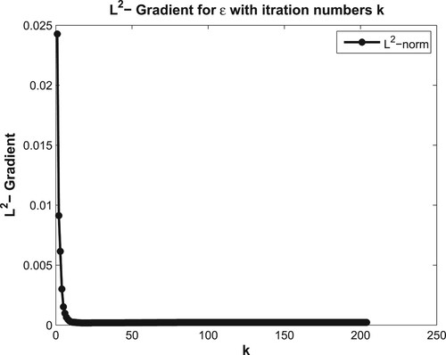Figure 4 shows the exact and reconstructed $\mathcal{E}$ for Example 7.2 at k = 34. At the first 25th iterations, the relative and residual errors are decreasing rapidly with increasing k, after which they decrease very slow till reach the minimizer (Figure 5). It should be noted that the approximated gradient direction becomes non-descent when k is greater than 25 (Figure 6). The solution of the EIIP in the proposed examples is quite stable to the perturbations of the input data using the proposed nonlinear conjugate gradient algorithm.

Figure 1. Exact and reconstructed ${\mathcal{E}}^k$ (left) and residual error of the coefficient (right) for Example 7.1 at $\eta =0.5\mathrm{\%}$ and $\mathcal{N}\mathcal{E}=\mathrm{20,000}$. The relative error $e_{\mathcal{E}}=0.023$ at k = 30.

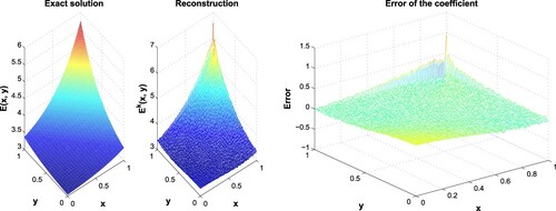
Figure 2. The variation of accuracy error (right) and residual error (left) corresponding to k for Example 7.1.

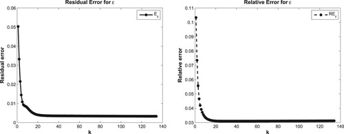
Table 1. The effect of the noise level on the identification parameter for Example 7.1.

$\mathcal{N}\mathcal{E}$	η (%)	k	$e_{\mathcal{E}}$	$\mathcal{J}$	$\mathcal{N}\mathcal{E}$	η (%)	k	$e_{\mathcal{E}}$	$\mathcal{J}$
1800	0.25	45	0.031	0.072	1800	1.50	6	0.049	0.183
1800	0.50	30	0.032	0.074	1800	1.75	5	0.054	0.24
1800	0.75	35	0.0355	0.097	1800	2.00	11	0.059	0.32
1800	1.00	16	0.0397	0.12	1800	2.25	5	0.065	0.47
1800	1.25	12	0.044	0.145	1800	2.50	10	0.071	0.70

Table 2. The numerical results (accuracy error) for Example 7.2.

k	$e_{\mathcal{E}}$	$\mathcal{J}$	k	$e_{\mathcal{E}}$	$\mathcal{J}$
1	0.111373	11.119523	38	0.023302	0.053117
5	0.053033	1.713813	64	0.021767	0.047584
10	0.032814	0.201715	107	0.020590	0.043443
25	0.025083	0.062509	202	0.019473	0.040174

Figure 3. Measurement data at different η, where (a) $\eta =5\mathrm{\%}$, (b) $\eta =1\mathrm{\%}$, and (c) $\eta =0.05\mathrm{\%}$ for Example 7.1.

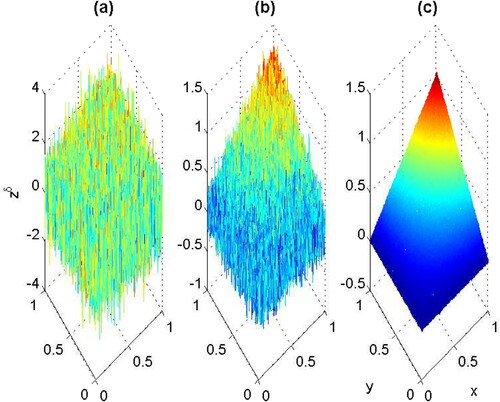
Figure 4. Exact and reconstruction ${\mathcal{E}}^k$ (left), residual error (right) at $k=34$ for Example 7.2, the relative error $e_{\mathcal{E}}=0.0128$ and $\mathcal{J}=0.000521$.

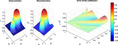
Figure 5. The variation of accuracy error (right) and residual error (left) corresponding to k for Example 7.2.

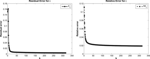
Figure 6. The convergence with $L^2$-gradient corresponding to k for Example 7.2.

7.1. Performance analysis and numerical comparison

To compare the proposed method with those in the literature, Jadamba et al's [19] example (Example 7.2) is considered first. Table 2 presents some features of Example 7.2 such as the accuracy error $e_{\mathcal{E}}$ and objective functional values $\mathcal{J}$ at different k. It is observed that at k = 38, a high accuracy is obtained, about $2\mathrm{\%}$, decreasing very slowly with increasing k (Table 2). These obtained results give a good agreement with those of Jadamba et al. [19] where they achieved a high accuracy for the algorithm after 139 and 49 iterations using the first-order adjoint method and the Newton method with a simple backtracking line search method, respectively. Second, another comparison is made with Jadamba et al. [19] (Example 6.1, [10]) at the same boundary conditions where the smooth coefficient is given as follows.

Example 7.3

The exact identification coefficient $\mathcal{E}(x,y)$ and load function $f(x,y)$ are given by (41) $\begin{array}{rl}\mathcal{E}(x,y)& =1-0.5\mathrm{sinc}\left[6\pi (x+{\displaystyle \frac{1}{10}})(y+\frac{1}{10})\right],f(x,y)=\left[\begin{array}{c}-{\displaystyle \frac{1}{5}}x\\ \cos (\pi x)\end{array}\right]\mathrm{in}\mathrm{\Omega },\\ g(x,y)& =\frac{1}{10}\left[\begin{array}{c}\sin (\pi y)\\ \sin (\pi x)\end{array}\right]\text{and}h(x,y)={\displaystyle \frac{1}{10}}\left[\begin{array}{c}1+10x\\ 1+10y\end{array}\right]\text{on}\mathrm{\partial }\mathrm{\Omega }\end{array}$(41) The function $g(x,y)$ represents the boundary condition on the bottom and left edges of Ω, and $h(x,y)$ is given on the top and right edges of Ω.

The proposed method is implemented on a $70\times 70$ mesh with 9800 total degrees of freedom at $\eta =0.001$. The residual error is defined as $E=\Vert {\mathcal{E}}_{\mathrm{computed}}-{\mathcal{E}}_{\mathrm{exact}}\Vert$. Figure 7 shows the variation of the residual error E corresponding to the starting point (initial guess ${\mathcal{E}}^0$), and the E values are compared with those obtained from the existing OLS function and the MOLS function introduced by Jadamba et al. [10]. This comparison was made with 50 trials chosen as constants to examine the sensitivity of $\mathcal{E}$ corresponding to ${\mathcal{E}}^0$. Figure 7 and Tables 2 and 3 show that a high level of accuracy with a small k is obtained using the proposed technique as compared to those in the previous work. The main advantages of this proposed method are presented as follows. First, the considered η can be increased upto $2.5\mathrm{\%}$, while the algorithm preserving the stability of the identification parameter (Table 1). Second, it has been numerically investigated that the recovered parameter reaches to the global minimum at a small k due to the convexity of the modified output least-squares method (Figure 7). The numerical results in this study show the efficiency and accuracy of the introduced algorithm. Figure 6 shows that the convergence rate of the $L^2$-gradient corresponding to k appears very steady. Jadamba et al. [10] considered the convergence rate of the MOLS function compared with that of the nonconvex OLS function. They found that the number of forward solutions which has connection with k decreases with increasing the mesh size. Following that test to examine the method performance, we increased the mesh size and examined the $e_{\mathcal{E}}$ and E, where one forward problem needs to be solved at each iteration. Table 3 compares $\mathcal{N}\mathcal{E}$, k, $e_{\mathcal{E}}$, E and elapsed time of the computations with those from Jadamba et al. [10]. The results show that, the accuracy and residual errors decrease with increasing the mesh size, showing a good agreement with those from [10]. We remark that, when ${\mathcal{E}}^0$ is far from the minimizer, more iterations are required to reach the global minimizer. Importantly, a good starting point should be chosen to determine the minimum k and computational cost.

Figure 7. A comparison of the residual error E using the present MOLS compared to that of Jadamba et al. [10] and the existing OLS at different starting points ${\mathcal{E}}^0$ for Example 7.3.

Table 3. Performance of the MOLS with increasing $\mathcal{N}\mathcal{E}$ for Example 7.3.

$\mathcal{N}\mathcal{E}$	k	$e_{\mathcal{E}}$	E	Elapsed time (s)
800	31	0.057595	0.057036	599
3200	89	0.043519	0.042320	6050
7200	68	0.039268	0.037950	16,304
12,800	67	0.038095	0.036702	53,964

8. Conclusions

In this paper, an efficient method is developed and implemented for identifying the modulus of elasticity, given a precise measurement data in the displacements. The proposed problem is motivated by potential applications to reconstruct the cancerous tumour in the EIIP. The variational formulation is applied for solving the forward problem using an approximation of the plane strain and plane stress conditions. The obtained results demonstrate the effectiveness and robustness of the proposed finite element method for solving the forward and the inverse problem. A new modified output least-squares (MOLS) functional is introduced. The sensitivity and adjoint problems are derived using Lagrange multipliers to obtain a new formula to compute the gradient using direct and adjoint approaches which are easier and not expensive in the computations. The nonlinear conjugate gradient method is implemented to solve the optimization inverse problem since the considered problem is highly ill-posed. Numerical experiments are provided to show that the numerical convergence is quite satisfactory for the proposed method as compared to those of the literature. The numerical results indicate that the radial basis functions as in the proposed experiments can efficiently represent the modulus of elasticity such as those occur in the soft tissue in the presence of tumors. The aforementioned performance analysis, numerical verification and comparisons indicate that the proposed algorithm is efficient, stable, and accurate. Yet, there are open problems for future works including simultaneously identifying Young's modulus and Poisson ratio in the elasticity imaging inverse problem. Moreover, hyperelasticity and large deformation models can be used to give a more accurate representation for reconstructing the elastic properties of the human soft tissues.

Disclosure statement

No potential conflict of interest was reported by the author(s).

Additional information

Funding

This work was supported by the Science and Technology Development Fund (STDF) of Egypt, project No: 39385. This research was supported in part by the National Key R&D Program of China under P2018YFE0198400, Shenzhen [grant number ZDSYS201703031711426], [grant number JCYJ20170818153840322], and NFSC [grant number 12071461].

References

- Smyl D, Antin K-N, Liu D, et al. Coupled digital image correlation and quasi-static elasticity imaging of inhomogeneous orthotropic composite structures. Inverse Probl. 2018;34(12):124005.
- Smyl D, Bossuyt S, Liu D. OpenQSEI: a MATLAB package for quasi static elasticity imaging. SoftwareX. 2019;9:73–76.
- Raghavan K, Yagle AE. Forward and inverse problems in elasticity imaging of soft tissues. IEEE Trans Nucl Sci. 1994;41(4):1639–1648.
- Doyley MM, Meaney PM, Bamber JC. Evaluation of an iterative reconstruction method for quantitative elastography. Phys Med Biol. 2000;45(6):1521–1540.
- Constantinescu A. On the identification of elastic moduli from displacement-force boundary measurements. Inverse Probl Eng. 1995;1:293–313.
- Dominguez N, Gibiat V, Esquerre Y. Time domain topological gradient and time reversal analogy: an inverse method for ultrasonic target detection. Wave Motion. 2005;42(1):31–52.
- Knopoff DA, Fernández D, Torres GA, et al. Adjoint method for a tumor growth PDE-constrained optimization problem. Comput Math Appl. 2013;66(6):1104–1119.
- Oberai AA, Gokhale NH, Feijóo GR. Solution of inverse problems in elasticity imaging using the adjoint method. Inverse Probl. 2003;19(2):297–313.
- Lozano C. Discrete surprises in the computation of sensitivities from boundary integrals in the continuous adjoint approach to inviscid aerodynamic shape optimization. Comput Fluids. 2012;56:118–127.
- Jadamba B, Khan A, Rus G, et al. A new convex inversion framework for parameter identification in saddle point problems with an application to the elasticity imaging inverse problem of predicting tumor location. SIAM J Appl Math. 2014;74(5):1486–1510.
- Parker KJ, Huang SR, Musulin RA, et al. Tissue response to mechanical vibrations for ‘sonoelasticity imaging’. Ultrasound Med Biol. 1990;16(3):241–246.
- Fehrenbach J, Masmoudi M, Souchon R, et al. Detection of small inclusions by elastography. Inverse Probl. 2006;22(3):1055–1069.
- Arnold A, Reichling S, Bruhns OT, et al. Efficient computation of the elastography inverse problem by combining variational mesh adaption and a clustering technique. Phys Med Biol. 2010;55(7):2035–2056.
- Ji L, McLaughlin J. Recovery of the Lamé parameter μ in biological tissues. Inverse Probl. 2003;20(1):1–24.
- McLaughlin JR, Yoon J-R. Unique identifiability of elastic parameters from time-dependent interior displacement measurement. Inverse Probl. 2003;20(1):25–45.
- Peltz JJ, Cacuci DG. Inverse predictive modeling of a spent fuel dissolver model. Nucl Sci Eng. 2016;184:1–15.
- Cacuci DG. Inverse predictive modeling of radiation transport through optically thick media in the presence of counting uncertainties. Nucl Sci Eng. 2017;186:199–223.
- Aguilo MA, Aquino W, Brigham JC, et al. An inverse problem approach for elasticity imaging through vibroacoustics. IEEE Trans Med Imaging. 2010;29:1012–1021.
- Jadamba B, Khan AA, Oberai AA, et al. First-order and second-order adjoint methods for parameter identification problems with an application to the elasticity imaging inverse problem. Inverse Probl Sci Eng. 2017;25:1768–1787.
- Babaniyi OA, Oberai AA, Barbone PE. Recovering vector displacement estimates in quasistatic elastography using sparse relaxation of the momentum equation. Inverse Probl Sci Eng. 2017;25(3):326–362.
- Abdelhamid T. Simultaneous identification of the spatio-temporal dependent heat transfer coefficient and spatially dependent heat flux using an MCGM in a parabolic system. J Comput Appl Math. 2018;328(9):164–176.
- Abdelhamid T, Deng X, Chen R. A new method for simultaneously reconstructing the space-time dependent Robin coefficient and heat flux in a parabolic system. Int J Numer Anal Model. 2017;14(6):893–915.
- Abdelhamid T, Elsheikh AH, Elazab A, et al. Simultaneous reconstruction of the time-dependent Robin coefficient and heat flux in heat conduction problems. Inverse Probl Sci Eng. 2018;26(9):1231–1248.
- Ammari H, Garapon P, Jouve F. Separation of scales in elasticity imaging: a numerical study. J Comput Math. 2010;28:354–370.
- Harrigana TP, Konofagou EE. Estimation of material elastic moduli in elastography: a local method, and an investigation of Poissons ratio sensitivity. J Biomech. 2004;37:1215–1221.
- Babuška I, Suri M. Locking effects in the finite element approximation of elasticity problems. Numer Math. 1992;62(1):439–463.
- Kwon YW, Bang H. The finite element method using MATLAB. London: CRC Press; 2000.
- Reddy JN. An introduction to the finite element method. Vol. 2, New York: McGraw-Hill; 1993.
- Gockenbach MS, Khan AA. Identification of Lamé parameters in linear elasticity: a fixed point approach. J Indust Manag Optim. 2005;1(4):487–497.
- Jadamba B, Khan AA, Raciti F. On the inverse problem of identifying Lamé coefficients in linear elasticity. Comput Math Appl. 2008;56(2):431–443.
- Cai Z, Starke G. Least-squares methods for linear elasticity. SIAM J Numer Anal. 2004;42:826–842.
- Houston DSP, Wihler TP. An hp-adaptive mixed discontinuous Galerkin FEM for nearly incompressible linear elasticity. Comput Methods Appl Mech Eng. 2006;195:3224–3246.
- Brezzi F, Fortin M. Mixed and hybrid finite element methods. New York: Springer-Verlag; 2012.
- Alifanov OM. Inverse heat transfer problems. Berlin: Springer Science & Business Media; 2012.
- Jarny Y, Ozisik M, Bardon J. A general optimization method using adjoint equation for solving multidimensional inverse heat conduction. Int J Heat Mass Transfer. 1991;34(11):2911–2919.
- Alifanov OM. Solution of an inverse problem of heat conduction by iteration methods. J Eng Phys Thermophys. 1974;26(4):471–476.
- Hansen P, O'Leary D. The use of the L-curve in the regularization of discrete ill-posed problems. SIAM J Sci Comput. 1993;14(6):1487–1503.
- Abdelhamid T, Elsheikh AH, Omisore OM, et al. Reconstruction of the heat transfer coefficients and heat fluxes in heat conduction problems. Math Comput Simul. 2021;187:134–154.
- Abdelhamid T, Chen R, Alam MM. Prediction of multi-parameters in the inverse heat conduction problems. J Phys: Conf Ser. 2020;1707:012003.