Cornering stiffness estimation using Levenberg–Marquardt approach

Abstract

Study of vehicle dynamics aggregates possibilities to enhance performance, safety and reliability, such as the integration of control systems, usually requiring knowledge on vehicle's states and parameters. However, some critical values are difficult to measure or are not disclosed. For this reason, dynamics and stability analysis of six-wheeled vehicles are compromised, and available information on this matter is limited. In this context, this paper proposes the estimation of the cornering stiffness of a 6x6 vehicle by an inverse problem approach applying the Levenberg–Marquardt (LM) method. The algorithm required data from field experiments and from simulations of a vehicle model during a double-lane change manoeuvre developed using ${\mathrm{S}\mathrm{i}\mathrm{m}\mathrm{u}\mathrm{l}\mathrm{i}\mathrm{n}\mathrm{k}}^{\circledR }/{\mathrm{M}\mathrm{A}\mathrm{T}\mathrm{L}\mathrm{A}\mathrm{B}}^{\circledR }$. Experimental and theoretical values for the vehicle yaw rate were combined through LM method for cornering stiffness estimation. The excellent agreement between measured and simulated yaw rate indicates that the proposed model and the estimated parameters properly represent the vehicle dynamics response.

Keywords:

• Vehicle dynamics
• cornering stiffness estimation
• Levenberg–Marquardt algorithm
• six-wheeled vehicle
• double-lane change manoeuvre

2010 Mathematics Subject Classifications:

• 37M05
• 70E99

1. Introduction

The addition of new or adapted technologies on a vehicle system contributes significantly to its performance improvement and safety. For that matter, mathematical and computer-aided models are widely applied in vehicle dynamics studies and vehicle control systems (VCS), since they allow parameters optimisation on a vehicle design, its dynamics behaviour prediction and resources and time saving. Therefore, the estimation of vehicle's states and parameters is considered in many researches [1,2], since it reduces uncertainties issues and it implies in a better agreement between the model and the real vehicle behaviour. According to [3,4], one of the interests of the academic community and automotive industries is the estimation of vehicle parameters to improve its performance and subsystems behaviour, particularly the ones which are complex or costly to measure, such as the cornering stiffness of the tyres.

As stated by Alatorre et al. [5] and Liu et al. [6], a deep knowledge of the system behaviour is fundamental to assure a satisfactory performance of an integrated control system, such as Advanced Driver Assistance Systems (ADAS) and lateral control strategies. A model-based approach is one of the main branches for controllers design, which requires the tracking and estimation of vehicle's states and parameters during manoeuvres. Based on this context, military vehicles are also facing developments in that direction [7]. According to [8,9], the vehicle behaviour and controllability are directly connected to lateral dynamics, which establish a vast field for estimations researches in this area. Therefore, this study aims to estimate the cornering stiffness parameters of a 6x6 three-axle military vehicle.

The tyres' cornering stiffness are complex to measure, since it requires specific equipment and procedures. Besides that, Van Eeden et al. [10] stated that they are dependent on many variables, such as tyre size and type, number of plies and wheel width. Also, Baffet et al. [11] indicated that the value of the cornering stiffness varies in the nonlinear tyre domain and also according to road friction. Its definition is related to a turning tyre under a vertical force F_z and a lateral force F_y. Due to tyres properties, an angular displacement in a region of the tyre tread occurs, known as slip angle α. For a small slip angle (α ⩽ 5°), its relation with the tyre lateral force is expressed by [12]: (1) $F_y=-C_{\alpha }\alpha .$(1) Therefore, the definition for cornering stiffness of a tyre is given by: (2) $C_{\alpha }=\underset{\alpha \to 0}{lim}\frac{\mathrm{\partial }(-F_y)}{\mathrm{\partial }\alpha }=∣\underset{\alpha \to 0}{lim}∣\frac{\mathrm{\partial }{F}_y}{\mathrm{\partial }\alpha }.$(2) However, outside the linear region, an appropriate non-linear tyre model must be applied, such as Pacejka, Dugoff or Brush models [1]. The last two, for instance, represent the longitudinal and lateral forces on the tyres using formulations based on the tyre longitudinal stiffness and cornering stiffness. Even though models with a constant cornering stiffness describe vehicle dynamics only during quasi-steady driving manoeuvres, commonly associated with an absolute lateral acceleration less than 0.4g (approximately 3.92 m s⁻²) on normal dry asphalts road [13], a nominal value for this parameter is still useful on controllers' design and tyre's model formulations. Some of the main reasons for that are the number of unknown parameters and the computational burden associated with complex and more accurate tyre models, specially during online vehicle control applications. Consequently, recent studies in this field considered a constant value for this parameter using a linear tyre model [14–16] or others that have considered its nominal value at an operation point [17–19].

According to Forte et al. [20], some tyre's properties are not available due to the intellectual property of the manufacturer. As a result, they are usually measured using expensive equipment, such as force transducers [21]. However, estimation with measurements of vehicle dynamics is quite attractive, and could be performed using an inertial measurement unit (IMU), which is a device mostly used for relative acceleration and angular rate measurement, and a Global Positioning System (GPS) [20]. Therefore, using available vehicle data, an inverse problem approach could be formulated in order to perform the estimation process. An inverse problem consists on the estimation of non-observed parameters of a mathematical formulation through dependent variables of the model. A number of important scientific and practical reliable results have been obtained through that approach, such as heat problems solutions, diagnostics of friction, and structure mechanics analysis [22].

Even though there are fewer studies on 6x6 wheeled vehicle when compared to on passenger cars, some investigations attempting to understand, simulate and control the dynamics of this type of vehicle have been conducted. The simple handling model (SHM) representation, commonly known as single-track or bicycle model, of a 6x6 vehicle was applied by An et al. [23] for yaw rate analysis and steering control. However, researches regarding the estimation of parameters are mostly related to two-axles vehicles and many studies were conducted using well-behaved measurements acquired from Carsim^TM [13,24–26], which is a professional vehicle simulation software, without considering the effect of noise during the process.

Several methods to estimate the cornering stiffness, both online and offline, are presented in the literature [1], such as Kalman filters and its variations [11,24,27–29], Recursive Least Squares (RLS) [13,30,31] and Neural Networks (NN) [2]. A review on techniques and strategies regarding vehicle dynamic state estimation presented in [1,2] pointed the single-track model as the mostly applied for vehicle lateral states estimation, while the main techniques performed to estimate the cornering stiffness were dual Kalman filter (DKF) and Extended Kalman Filter (EKF), both filter-based; RLS [31] and a non-linear observer (NLO), both observer-based, considering a single-track together with a linear tyre model. Regarding the application of NN, Singh et al. [32] highlight that the estimated results are satisfactory within the constraints of the trained operation conditions. However, new experimental measurements would have to be acquired if one of the vehicle's characteristics changed, such as its mass and the tyres.

The study presented in [25] considered the vehicle lateral/yaw dynamics to estimate the road friction and cornering stiffness parameters assuming an SHM for a two-axle vehicle, on the basis that estimation methods using vehicle's motion data are more robust than the ones based on tyres dynamics behaviour. Another advantage of using the measured signals is that they are readily measured for other purposes, such as accelerations and angles rates during vehicle performance assessment. The work developed in [26] used a Dual Unscented Kalman Filter (DUKF) to identify the lateral forces, sideslip angles and normal forces, while Pacejka's tyre coefficients were estimated using a hybrid Levenberg–Marquardt (LM) and quasi-Newton method. The cornering stiffness and the friction coefficient were simultaneously identified in [33] using a Lyapunov based adaptive law and a single-track vehicle model with Carsim^TM measurements.

The LM algorithm has already been implemented as an optimization method for vehicle dynamics analysis and tested using measurements from a realistic simulator called CALLAS for maximum lateral friction coefficient estimation in [34,35]. The tyre/road interaction, reflected as tyre lateral force, considered a nonlinear Dugoff model available in CALLAS. It required several output information of a vehicle's motion, such as yaw and roll rate, longitudinal and lateral acceleration and steering angle. An identification technique based on the LM method was applied in [36] to obtain the membership function parameters used in the rules of a Takagi–Sugeno (T-S) fuzzy model, which included the front and rear cornering stiffness, using a bicycle model, while the lateral forces on the front and rear tyres were expressed by Pacejka's Magic Formula.

The LM algorithm is a fast method and has stable convergence for minimizing a nonlinear function [37], such as formulations for vehicle dynamics. Through an iterative best fit process between measured and modelled data, the estimation of parameters is performed. Besides, its implementation is not complex, and not many information is needed for the intended model objective. Also, Lourakis et al. [38] stated that the LM method is considered a standard technique for nonlinear least-squares problems, applied in several scientific areas. However, none of the previous work presented a method for the cornering stiffness estimation of a three-axle vehicle, specially regarding military vehicles, whose tyres sizes are usually bigger than of passenger cars, and information about its properties are limited due to intellectual property policy and the sparse amount of available studies in this matter. Furthermore, the LM approach for cornering stiffness estimation directly has not been performed yet, only applied together with other techniques.

Therefore, in cases where experimental measurements of a vehicle are available, this paper proposes an alternative to estimate the cornering stiffness parameters that satisfy the mathematical relations given by the proposed model of a specific 6x6 vehicle applying the LM algorithm. Moreover, experimental data of a tested vehicle during a double-lane change manoeuvre were applied to perform this process, making it possible to compare the numerical solution to the yaw rate measurements. The main contributions of this paper are: (1) the estimation of the nominal cornering stiffness parameters of a three-axle military vehicle; (2) the application of the LM algorithm in the estimation process; and (3) the use of experimental field measurements of a three-axle military vehicle in the estimation process.

The remainder of this paper is structured as follows: Section 2 explains the experimental measurements acquisition. The forward problem is stated in Section 3, introducing the well-known SHM (single-track/bicycle model) for a two-axle vehicle, and extending the mathematical formulation for a three-axle model. The LM algorithm applied in this study and a sensibility analysis with the intended cornering stiffness parameters is performed in Section 4. Estimation results using simulated measurements initially, followed by the same process applied to Carsim^TM data and experimental measurements of a tested vehicle are presented and discussed in Section 5. Conclusions and future studies are stated in Section 6.

2. Experimental measurements

Manoeuvres such as lane changes [26,27,31], slalom [11,13], J-turn [25] and step steer [9,26] are usually applied to perform states and parameters estimation associated with vehicle lateral dynamics. Therefore, since the double-lane change is usually performed to evaluate lateral stability, the standard North Atlantic Treaty Organization (NATO) double-lane change, presented in the Allied Vehicle Testing Publications (AVTP) 03-160 W [39], was selected for the acquisition of the necessary experimental measurements to further apply the inverse problem analysis and the cornering stiffness estimation.

It is important to highlight that military vehicles must be compliant with operational and technical requirements, and the double-lane change manoeuvre is performed in Brazilian military vehicles because it simulates a condition where the vehicle must deviates an obstacle, such as anti-car mine explosion, that could block the vehicle's path on the battlefield. This manoeuvre is also frequently applied by Tank Automotive Research Development and Engineering Center (TARDEC), an organization of the United States Army [40].

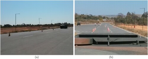
The manoeuvre consists in the transition from a right lane to a left lane, and the return to the initial right lane afterwards. According to this procedure, this test must be repeated with a constant velocity, and at each new trial, the velocity is increased until the driver is no longer confident on the vehicle's stability, the maximum speed planned for the test is reached or if it not possible to perform the track without knocking the cones down. In agreement with [39], a test track was set up according to the lay-out given in Figure 1 and Table 1. Cones were used for marking lanes and distances based on the vehicle dimensions given in Table 2. The 6x6 armoured vehicle selected for real-time experimental data acquisition is presented in Figure 2.

Figure 1. Double-lane change track.

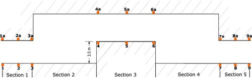
Figure 2. Vehicle used for experimental measurements.

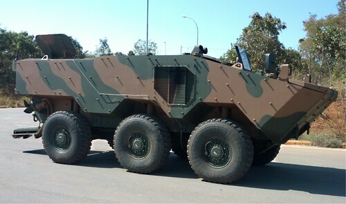
Table 1. Lane change track dimensions in agreement with [39].

Section	Length	Width
Section 1	15 m	1.1(vehicle width)+0.25 m
Section 2	Overall length of vehicle^a + 24 m	–
Section 3	25 m	1.2(vehicle width)+0.25 m
Section 4	Overall length of vehicle^a + 24 m	–
Section 5	15 m	1.1(vehicle width)+0.25 m

Note: ${}^a$ Overall length of vehicle, measured at 0.50 m from the ground.

Table 2. Vehicle's information.

Mass	m	15,770 kg
Length	L	7.100 m
Maximum height	H	2.600 m
Maximum width	$w_v$	3.300 m
Track	w	2.260 m
Wheelbase	l	3.700 m
Distance from c.g. to front axle	$a_1$	1.7746 m
Distance from c.g. to middle axle	$a_2$	0.0746 m
Distance from c.g. to rear axle	$a_3$	1.9254 m
Moment of inertia (z-axis)	$I_z$	63,595 kg m^2
Tyre	–	14.00R20
Tyre inflation pressure	$P_{\mathrm{t}\mathrm{y}\mathrm{r}\mathrm{e}}$	500 kPa

Tests were performed on a test track, and the measurements data, such as longitudinal velocity, pitch, roll and yaw rate, were collected using the following equipment:

• Data logger VBOX 3i for automotive applications from Racelogic®;

• Inertial Measurement Unit (IMU) model RLVBIMU04 from Racelogic®;

• GPS antenna; and

• Draw wire displacement sensor of 500 mm of measuring range used in automotive engineering from MICRO-EPSILON®.

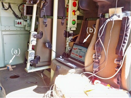
The IMU provides measurements of pitch, roll and yaw rates using three rate gyros, as well as x, y, z acceleration via three accelerometers. This device was fixed on the floor of the troop compartment, as close as possible to the vehicle's centre of mass, calculated from its computer-aided design model (CAD), and set up in order to match its axis with the vehicle coordinate system established, supposing that they were exactly aligned. According to IMU user guide [41], the resolution for rate sensors is 0.01°/s.

The linear displacement transducer mounted in the auxiliary steering cylinder (front left wheel) was used to obtain a linear function relating the angle of the driver's steering wheel and the steer on the front left tyre. Starting from the neutral position, the output voltage of the transducer was recorded as the driver's steering wheel was turned to the left and right lock at each ${10}^{\circ }$ increment, according to Figure 3. The transducer and IMU were connected to the VBOX 3i, which was responsible for logging CAN data from the vehicle: the IMU via CAN port and the linear transducer via the analogue output port. A GPS antenna was also fixed on the external top of the vehicle for distance travelled and velocity acquisition. Lastly, VBOX was plugged via an Universal Serial Bus (USB) port to a Panasonic® toughbook. Figure 4 illustrates the experimental set-up inside the vehicle.

Figure 3. Driver's steering wheel setup for angle measurements.

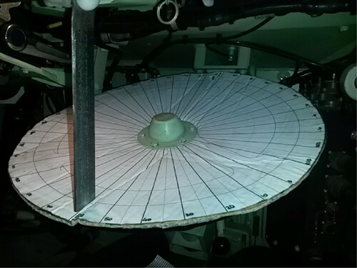
Figure 4. Experiment set-up inside the vehicle. (a) IMU position. (b) Toughbook rugged laptop for online data log.

For the double-lane change experiment, the track was set up according to [39] as shown in Figure 5. An unladen vehicle performed double-lane changes manoeuvres at 10 km h⁻¹, 20 km h⁻¹, 30 km h⁻¹, 40 km h⁻¹, 50 km h⁻¹ and 60 km h⁻¹, and the data capturing equipment was initiated and stopped at each new trial for successive increase in speed. Data were recorded at 100 Hz and saved for subsequent analysis.

Figure 5. Vehicle during a lane change test. (a) External view of the vehicle. (b) Driver view (open hatch).

Data preprocessing before applying them to estimate parameters is important to compensate for disturbances in the sensors, mainly due to inevitable noise related to the vehicle's vibration when the engine is running, road irregularities and sensors offset. As stated by Nirmal et al. [42], errors in IMU response can be deterministic or stochastic. The first type refers to errors that remain either constant or its variation over time can be determined, such as static biases, sensor misalignment and scale factor, which can be calibrated. The latter are based on random processes, and are difficult to model, such as measurement noise, drifting biases.

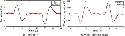
The variables of interest in this study are the yaw rate, the wheel steering angle and lateral acceleration of the vehicle performing a double-lane change manoeuvre at 10 km h⁻¹. The yaw rate was selected for the estimation process because its measured values are more reliable in comparison to the lateral acceleration. The wheel steering angle was used as an input to the vehicle's computer model (forward problem formulation) in order to apply the same input manoeuvre. The values of the lateral acceleration and the manoeuvre at 10 km h⁻¹ were considered to maintain the tyres in the linear region.

A low-pass filter of 2.5 Hz was applied using a minimum-order filter with a stop-band attenuation of 60 dB and compensation for the delay introduced by the filter. The low-pass was applied to remove high-frequency content from other sources, such as noise and vehicle's vibration, and the pass-band frequency. The sensor offset was significant in the measurements of the wheel steering angle and the lateral acceleration, resultant from the sensors positioning and calibration. Therefore, pre-test data were applied in the signals to remove it. Figure 6 shows the raw data and filtered measurements after signals post-processing.

Figure 6. Filtered measurements.

3. Physical problem and mathematical formulation

3.1. Vehicle lateral dynamics

3.1.1. Plane model

There are several well-established vehicle models, chosen usually based on their complexity of implementation, required variables and motion of study. Therefore, the decision of which to use commonly lies on the complexity and information provided by the dynamic model. Vehicle dynamics is usually divided into three main areas:

• Longitudinal dynamics: related to the vehicle dynamics that generate forward motion, such as acceleration and braking performance;

• Vertical dynamics: related to the spectrum of vibration that the car is subjected due to excitation sources, such as road roughness and driveline [43]. Frequencies and modes of vibration, such as bounce and pitch movements of a vehicle, and also ergonomics can be investigated for instance. It is usually referred as ride evaluation;

• Lateral dynamics: studies the vehicle behaviour in curves driving. According to Van Eeden et al. [10], the cornering behaviour of a vehicle is usually considered as a critical performance mode such as handling, which is related to the vehicle response to a driver input.

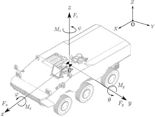
Since an initial dynamics study is necessary, formulations based on Newton–Euler equations of a body are frequently applied in a convenient and in a global coordinate system. Therefore, in order to illustrate the vehicle position and orientation, it was adopted a body coordinate system Cxyz (C is the mass centre of the vehicle), measured with respect to a grounded fixed coordinate frame OXYZ presented in Figure 7. The vehicle orientation is given by the roll angle φ about the x-axis, pitch angle θ about the y-axis and yaw angle ψ about the z-axis. Since the rate of the orientation angles are important parameters in vehicle dynamics, the following notation is commonly used: roll rate $\dot{\phi }=p$, pitch rate $\dot{\theta }=q$ and yaw rate $\dot{\psi }=r$.

Figure 7. Vehicle coordinate system Cxyz in a global coordinate frame OXYZ in accordance with ISO 4130.

According to [12], when the longitudinal, lateral and angular velocities are necessary and sufficient to examine the vehicle behaviour, a plane model is applicable. Regarding planar lateral vehicle dynamics, the vehicle could be considered as a rigid body with three degrees of freedom (DoF): translation in the x- and y-directions, and a rotation around the z-axis. Equations (3(3) $\begin{array}{rl}{F}_x& =m{\dot{v}}_x-mr{v}_y,\end{array}$(3) )–(5(5) $\begin{array}{rl}{M}_z& =\dot{r}{I}_z,\end{array}$(5) ) represent Newton–Euler equations of motions for a rigid vehicle defined according to the body coordinate frame Cxyz [12]: (3) $\begin{array}{rl}{F}_x& =m{\dot{v}}_x-mr{v}_y,\end{array}$(3) (4) $\begin{array}{rl}{F}_y& =m{\dot{v}}_y+mr{v}_x,\end{array}$(4) (5) $\begin{array}{rl}{M}_z& =\dot{r}{I}_z,\end{array}$(5) where F_x is the longitudinal force (along x-axis); F_y is is the lateral force (along y-axis); v_x is the longitudinal velocity of the vehicle; v_y is the lateral velocity of the vehicle; I_z is the vehicle mass moment of inertia about the z-axis; m is the vehicle mass; r is the yaw rate ($\dot{\psi }$); M_z is the yaw moment.

Since the force systems are defined initially at the tyreprint of the wheels, it is necessary to transform and apply the tyre force systems on the body of the vehicle in order to ensure that they are applied on the body centre of mass. Based on Figure 8, forces and moments are represented in x_wy_w-plane, x₁y₁-plane and xy-plane coordinate systems of the wheel, wheel-body and vehicle frame, respectively, for wheel number 1 (considered as the front left wheel). Generalizing for any wheel number i, the components of the force system in the xy-plane applied on a rigid vehicle due to the generated forces at the tyreprint of wheel i are given by Equations (6(6) $\begin{array}{rl}{F}_{x_i}& =F_{x_{{\omega }_i}}\cos \left({\delta }_i\right)-F_{y_{{\omega }_i}}\sin \left({\delta }_i\right),\end{array}$(6) )–(8(8) $\begin{array}{rl}{M}_{z_i}& =M_{z_{{\omega }_i}}+x_i{F}_{y_i}-y_i{F}_{x_i}.\end{array}$(8) ) [12]: (6) $\begin{array}{rl}{F}_{x_i}& =F_{x_{{\omega }_i}}\cos \left({\delta }_i\right)-F_{y_{{\omega }_i}}\sin \left({\delta }_i\right),\end{array}$(6) (7) $\begin{array}{rl}{F}_{y_i}& =F_{y_{{\omega }_i}}\cos \left({\delta }_i\right)+F_{x_{{\omega }_i}}\sin \left({\delta }_i\right),\end{array}$(7) (8) $\begin{array}{rl}{M}_{z_i}& =M_{z_{{\omega }_i}}+x_i{F}_{y_i}-y_i{F}_{x_i}.\end{array}$(8) Therefore, the total planar force system on the rigid vehicle in the body coordinate frame is given by the sum expression of Equations (6(6) $\begin{array}{rl}{F}_{x_i}& =F_{x_{{\omega }_i}}\cos \left({\delta }_i\right)-F_{y_{{\omega }_i}}\sin \left({\delta }_i\right),\end{array}$(6) )–(8(8) $\begin{array}{rl}{M}_{z_i}& =M_{z_{{\omega }_i}}+x_i{F}_{y_i}-y_i{F}_{x_i}.\end{array}$(8) ) considering all wheels, which is expressed by Equations (9(9) $\begin{array}{rl}{}^c{F}_x& =\sum _i{F}_{x_{{\omega }_i}}\cos \left({\delta }_i\right)-\sum _i{F}_{y_{{\omega }_i}}\sin \left({\delta }_i\right),\end{array}$(9) )–(11(11) $\begin{array}{rl}{M}_z& =\sum _i{M}_{z_{{\omega }_i}}+\sum _i{x}_i{F}_{y_i}-\sum _i{y}_i{F}_{x_i}.\end{array}$(11) ): (9) $\begin{array}{rl}{}^c{F}_x& =\sum _i{F}_{x_{{\omega }_i}}\cos \left({\delta }_i\right)-\sum _i{F}_{y_{{\omega }_i}}\sin \left({\delta }_i\right),\end{array}$(9) (10) $\begin{array}{rl}{}^c{F}_y& =\sum _i{F}_{y_{{\omega }_i}}\cos \left({\delta }_i\right)+\sum _i{F}_{x_{{\omega }_i}}\sin \left({\delta }_i\right),\end{array}$(10) (11) $\begin{array}{rl}{M}_z& =\sum _i{M}_{z_{{\omega }_i}}+\sum _i{x}_i{F}_{y_i}-\sum _i{y}_i{F}_{x_i}.\end{array}$(11) According to [13], the tyre lateral force depends on the tyre slip angle α, the road adhesion coefficient and the wheel load. The tyre slip angle is defined as the angle between its direction of heading and its direction of travel [43]. Figure 9 illustrates the usual relation between the lateral force and the slip angle, where the slope of the linear region is equivalent to the magnitude of the tyre cornering stiffness, as previously expressed by Equation (2(2) $C_{\alpha }=\underset{\alpha \to 0}{lim}\frac{\mathrm{\partial }(-F_y)}{\mathrm{\partial }\alpha }=∣\underset{\alpha \to 0}{lim}∣\frac{\mathrm{\partial }{F}_y}{\mathrm{\partial }\alpha }.$(2) ). According to [43,44], $F_y$ is also known as cornering force when the camber angle is zero.

Figure 8. The force system at the tyreprint of wheel number 1.

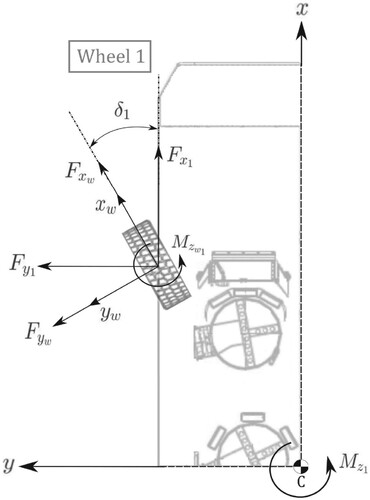
Figure 9. Slip angle x tyre lateral force.

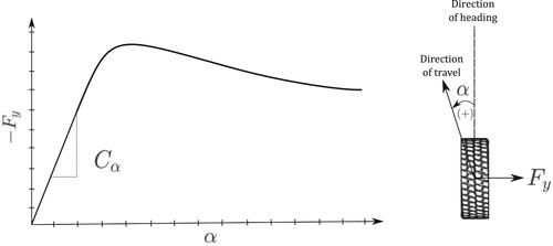
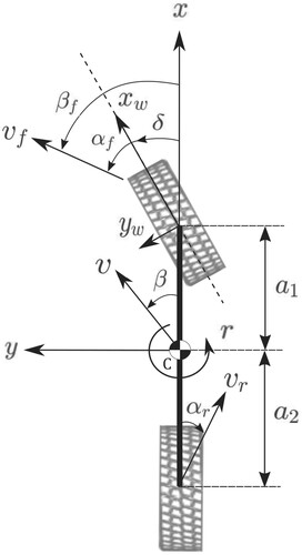
For tyre slip angle calculation, the angular orientation of a moving tyre is presented in Figure 10. Given the steer angle δ, and the sideslip angle β, defined as the angle between the velocity vector $\mathit{v}$ and the x-axis of the vehicle, the slip angle α can be expressed by Equation (12(12) $\alpha =\text{β}-\delta .$(12) ) [12]: (12) $\alpha =\text{β}-\delta .$(12)

Figure 10. Angular orientation of a moving tyre along the velocity vector $\mathit{v}$ at a slip angle α and a steer angle δ (adapted from [12]). (a) α, β and δ are positive. (b) $\text{β}<\delta$, thus α is negative.

For small values of the angle α (5° or less [43]), a linear tyre model is usually assumed, and Equation  (1(1) $F_y=-C_{\alpha }\alpha .$(1) ) is simplified for each tyre as shows Equation  (13(13) $F_y=-C_{\alpha }\alpha =-C_{\alpha }(\text{β}-\delta ).$(13) ) [12]: (13) $F_y=-C_{\alpha }\alpha =-C_{\alpha }(\text{β}-\delta ).$(13) Regarding the necessary angles for Equation (13(13) $F_y=-C_{\alpha }\alpha =-C_{\alpha }(\text{β}-\delta ).$(13) ), the steer angle δ is a function of the vehicle trajectory, and is usually used as a input for the movements equations. Additionally, the sideslip angle β_i is given by the geometry of each wheel i as can be seen in Figure 10 and its value is calculated from Equation (14(14) ${\text{β}}_i={\tan }^{-1}\left(\frac{v_{y_i}}{v_{x_i}}\right)={\tan }^{-1}\left(\frac{v_y+x_{i}r}{v_x-y_{i}r}\right).$(14) ): (14) ${\text{β}}_i={\tan }^{-1}\left(\frac{v_{y_i}}{v_{x_i}}\right)={\tan }^{-1}\left(\frac{v_y+x_{i}r}{v_x-y_{i}r}\right).$(14)

3.1.2. Simple handling model (SHM)

Although more complex vehicle dynamics models are available, many studies make use of simplified models since they are easier to implement and considered satisfactory at low to moderate lateral acceleration [10,20]. Ignoring the roll motion of the vehicle, the xy-plane remains parallel to the road's XY-plane, and the model is reduced by considering only one wheel per axle. This simple handling model is also known as the bicycle model [45] or single-track model [20], and it is illustrated in Figure 11 for a two-axle vehicle, where a₁ and a₂ are the distances of the front and the rear wheels to the centre of mass of the vehicle, respectively.

Figure 11. SHM for a two-axle vehicle moving with no roll.

SHM is usually used to model and describe the lateral dynamics of a vehicle, especially yaw rate (r) and sideslip angle (β). It allows the analysis of the vehicle behaviour subjected to traction forces, the influence of the distance between steering axles and their different configurations, and even the stability study during a steady-state turning, making it possible to classify the vehicle response as understeer (stable), neutral or oversteer (unstable). Since the two wheels in each axle are replaced by an ‘equivalent’ wheel, the axles cornering stiffness are expressed, as a consequence, by Equations (15(15) $\begin{array}{rl}{C}_{{\alpha }_f}& =C_{{\alpha }_{f_L}}+C_{{\alpha }_{f_R}},\end{array}$(15) ) and (16(16) $\begin{array}{rl}{C}_{{\alpha }_r}& =C_{{\alpha }_{r_L}}+C_{{\alpha }_{r_R}},\end{array}$(16) ) [12]: (15) $\begin{array}{rl}{C}_{{\alpha }_f}& =C_{{\alpha }_{f_L}}+C_{{\alpha }_{f_R}},\end{array}$(15) (16) $\begin{array}{rl}{C}_{{\alpha }_r}& =C_{{\alpha }_{r_L}}+C_{{\alpha }_{r_R}},\end{array}$(16) where C_αf is the effective front cornering stiffness; C_αfL is the front left tyre cornering stiffness; C_αfR is the front right tyre cornering stiffness; C_αr is the effective rear cornering stiffness; C_αrL is the rear left tyre cornering stiffness; C_αrR is the rear right tyre cornering stiffness.

In addition, considering that only the front wheel is steerable, Equations of motion (9(9) $\begin{array}{rl}{}^c{F}_x& =\sum _i{F}_{x_{{\omega }_i}}\cos \left({\delta }_i\right)-\sum _i{F}_{y_{{\omega }_i}}\sin \left({\delta }_i\right),\end{array}$(9) )–(11(11) $\begin{array}{rl}{M}_z& =\sum _i{M}_{z_{{\omega }_i}}+\sum _i{x}_i{F}_{y_i}-\sum _i{y}_i{F}_{x_i}.\end{array}$(11) ) are simplified and expressed by Equations (17(17) $\begin{array}{rl}{F}_x& =F_{x_f}\cos \left(\delta \right)+F_{x_r}-F_{y_f}\sin \left(\delta \right),\end{array}$(17) )–(19(19) $\begin{array}{rl}{M}_z& =a_1{F}_{y_f}-a_2{F}_{y_r}.\end{array}$(19) ): (17) $\begin{array}{rl}{F}_x& =F_{x_f}\cos \left(\delta \right)+F_{x_r}-F_{y_f}\sin \left(\delta \right),\end{array}$(17) (18) $\begin{array}{rl}{F}_y& =F_{y_f}\cos \left(\delta \right)+F_{y_r}+F_{x_f}\sin \left(\delta \right),\end{array}$(18) (19) $\begin{array}{rl}{M}_z& =a_1{F}_{y_f}-a_2{F}_{y_r}.\end{array}$(19) Moreover, the sideslip angle of each wheel may be calculated applying Equation (14(14) ${\text{β}}_i={\tan }^{-1}\left(\frac{v_{y_i}}{v_{x_i}}\right)={\tan }^{-1}\left(\frac{v_y+x_{i}r}{v_x-y_{i}r}\right).$(14) ) for the front and the rear wheels, resulting in Equations (20(20) $\begin{array}{rl}{\text{β}}_f& ={\tan }^{-1}\left(\frac{v_y+a_{1}r}{v_x}\right),\end{array}$(20) ) and (21(21) $\begin{array}{rl}{\text{β}}_r& ={\tan }^{-1}\left(\frac{v_y-a_{2}r}{v_x}\right).\end{array}$(21) ): (20) $\begin{array}{rl}{\text{β}}_f& ={\tan }^{-1}\left(\frac{v_y+a_{1}r}{v_x}\right),\end{array}$(20) (21) $\begin{array}{rl}{\text{β}}_r& ={\tan }^{-1}\left(\frac{v_y-a_{2}r}{v_x}\right).\end{array}$(21) Therefore, it is possible to calculate the lateral force for each wheel using Equation (13(13) $F_y=-C_{\alpha }\alpha =-C_{\alpha }(\text{β}-\delta ).$(13) ). Furthermore, as the main objective is the simulation of a vehicle during a double-lane change manoeuvre at a constant speed, Equation (3(3) $\begin{array}{rl}{F}_x& =m{\dot{v}}_x-mr{v}_y,\end{array}$(3) ) for the longitudinal force can be simplified and expressed by Equation (22(22) $F_x=-mr{v}_y.$(22) ): (22) $F_x=-mr{v}_y.$(22) Subsequently, for an SHM with no roll motion, it may be assumed that the system inputs are the steer angle δ, parameters associated with the vehicle and v_x. The resultant output considered is v_y and r. It is important to highlight some assumptions made for the SHM application:

• Constant vehicle velocity;

• No lateral or longitudinal load transfer, consequently the vehicle roll and pitch movements are not considered;

• Planar model;

• Use of a linear tyre model, whose reliability range occurs for small slip angles, and at low lateral acceleration and velocity;

• Cornering stiffness considered constant.

3.2. Forward problem formulation for a 6x6 vehicle

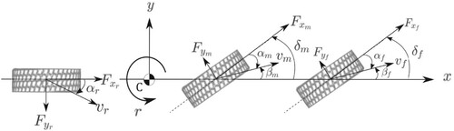
In order to analyse the lateral dynamics of a 6x6 vehicle, the SHM of a 3-axle, 1-rigid body ground vehicle is proposed in Figure 12, considering that the front and the middle axles are steerable with angles δ_f and δ_m, respectively, and disregarding the roll motion and other parameters such as ride motion (e.g. pitch and bounce), which affect the real behaviour of a vehicle.

Figure 12. Schematic representation of the SHM for a three-axle vehicle.

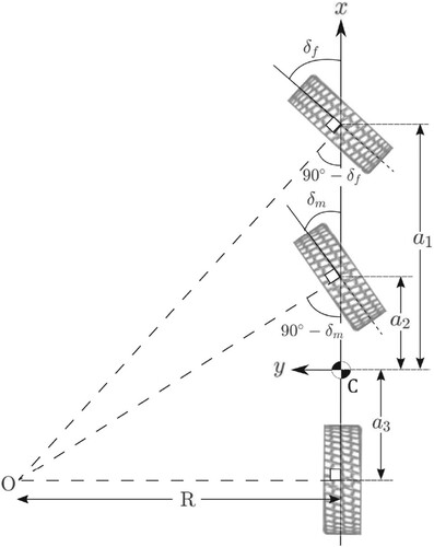
The steer angle of the front axle δ_f is associated with the driver's steering wheel input. For low speed turning, the geometry of a manoeuvre during curves may be designed according to the Ackermann condition. As stated by Van Eeden et al. [10], when steering the first and middle axles, the turning point can be defined as the intersection of the line parallel to the rear axle, with the lines perpendicular to the steering wheels as illustrated in Figure 13. Using the Ackermann condition and based on the vehicle's geometry, it is possible to obtain the relation between δ_f and δ_m given by Equation (23(23) ${\delta }_m={\tan }^{-1}\left(\frac{a_3+a_2}{a_3+a_1}\tan \left({\delta }_f\right)\right),$(23) ): (23) ${\delta }_m={\tan }^{-1}\left(\frac{a_3+a_2}{a_3+a_1}\tan \left({\delta }_f\right)\right),$(23) where a₁, a₂ and a₃ are the distances of the centre of mass of the vehicle to the front, middle and rear axles, respectively. The vehicle equations of motion are similar to the previously presented for a two-wheel model in Section 3.1.2. Combining an analogous formulation to Equations (17(17) $\begin{array}{rl}{F}_x& =F_{x_f}\cos \left(\delta \right)+F_{x_r}-F_{y_f}\sin \left(\delta \right),\end{array}$(17) )–(19(19) $\begin{array}{rl}{M}_z& =a_1{F}_{y_f}-a_2{F}_{y_r}.\end{array}$(19) ) for a front and middle wheel-steering three-axle vehicle with Equations (3(3) $\begin{array}{rl}{F}_x& =m{\dot{v}}_x-mr{v}_y,\end{array}$(3) )–(5(5) $\begin{array}{rl}{M}_z& =\dot{r}{I}_z,\end{array}$(5) ), it is possible to describe the vehicle motion on the reference system of the body. According to Section 2, during a double-lane change manoeuvre, it is assumed constant speed (${\dot{v}}_x=0$), thus Equation (22(22) $F_x=-mr{v}_y.$(22) ) can be applied. Therefore, the final simplified mathematical formulation for the vehicle dynamics is given by Equation (24(24) $\left[\begin{array}{c}{\dot{v}}_y\\ \\ \dot{r}\end{array}\right]=\left[\begin{array}{cccccc}\frac{\sin \left({\delta }_f\right)}{m}& \frac{\cos \left({\delta }_f\right)}{m}& \frac{\sin \left({\delta }_m\right)}{m}& \frac{\cos \left({\delta }_m\right)}{m}& 0& \phantom{-}\frac{1}{m}\\ \\ \frac{a_1\sin \left({\delta }_f\right)}{I_z}& \frac{a_1\cos \left({\delta }_f\right)}{I_z}& \frac{a_2\sin \left({\delta }_m\right)}{I_z}& \frac{a_2\cos \left({\delta }_m\right)}{I_z}& 0& -\frac{a_3}{I_z}\end{array}\right]\left[\begin{array}{c}{F}_{x_f}\\ F_{y_f}\\ F_{x_m}\\ F_{y_m}\\ F_{x_r}\\ F_{y_r}\end{array}\right]-\left[\begin{array}{c}r{v}_x\\ \\ 0\end{array}\right]$(24) ): (24) $\left[\begin{array}{c}{\dot{v}}_y\\ \\ \dot{r}\end{array}\right]=\left[\begin{array}{cccccc}\frac{\sin \left({\delta }_f\right)}{m}& \frac{\cos \left({\delta }_f\right)}{m}& \frac{\sin \left({\delta }_m\right)}{m}& \frac{\cos \left({\delta }_m\right)}{m}& 0& \phantom{-}\frac{1}{m}\\ \\ \frac{a_1\sin \left({\delta }_f\right)}{I_z}& \frac{a_1\cos \left({\delta }_f\right)}{I_z}& \frac{a_2\sin \left({\delta }_m\right)}{I_z}& \frac{a_2\cos \left({\delta }_m\right)}{I_z}& 0& -\frac{a_3}{I_z}\end{array}\right]\left[\begin{array}{c}{F}_{x_f}\\ F_{y_f}\\ F_{x_m}\\ F_{y_m}\\ F_{x_r}\\ F_{y_r}\end{array}\right]-\left[\begin{array}{c}r{v}_x\\ \\ 0\end{array}\right]$(24) For a plane model and considering small steering angles, the traction force F_x applied may be approximated by Equation (25(25) $F_x\approx F_{x_f}+F_{x_m}+F_{x_r}.$(25) ) [12]: (25) $F_x\approx F_{x_f}+F_{x_m}+F_{x_r}.$(25) Thus, assuming that traction is equally distributed between the vehicle axles, the longitudinal force in each axle is given by Equation (26(26) $F_{x_f}=F_{x_m}=F_{x_r}=-\frac{mr{v}_y}{3}.$(26) ): (26) $F_{x_f}=F_{x_m}=F_{x_r}=-\frac{mr{v}_y}{3}.$(26) Assuming small and equal tyre slip angles on the left and the right wheels [23] for each axle, the lateral force in the ‘equivalent’ wheel is obtained by Equation (13(13) $F_y=-C_{\alpha }\alpha =-C_{\alpha }(\text{β}-\delta ).$(13) ), applying the resultant cornering stiffness parameters for an SHM (as expressed by Equations (15(15) $\begin{array}{rl}{C}_{{\alpha }_f}& =C_{{\alpha }_{f_L}}+C_{{\alpha }_{f_R}},\end{array}$(15) ) and (16(16) $\begin{array}{rl}{C}_{{\alpha }_r}& =C_{{\alpha }_{r_L}}+C_{{\alpha }_{r_R}},\end{array}$(16) )): (27) $\begin{array}{rl}{F}_{y_f}& =-C_{{\alpha }_f}({\text{β}}_f-{\delta }_f),\end{array}$(27) (28) $\begin{array}{rl}{F}_{y_m}& =-C_{{\alpha }_m}({\text{β}}_m-{\delta }_m),\end{array}$(28) (29) $\begin{array}{rl}{F}_{y_r}& =-C_{{\alpha }_r}{\text{β}}_r,\end{array}$(29) where: (30) ${\text{β}}_f={\tan }^{-1}\left(\frac{v_y+a_{1}r}{v_x}\right),$(30) (31) ${\text{β}}_m={\tan }^{-1}\left(\frac{v_y+a_{2}r}{v_x}\right),$(31) (32) ${\text{β}}_r={\tan }^{-1}\left(\frac{v_y-a_{3}r}{v_x}\right).$(32) C_αf, C_αm and C_αr are the cornering stiffness of the front, middle and rear ‘equivalent’ tyres (or axles), respectively, for the SHM proposed in Figure 12. Since the measurement of the cornering stiffness is a complex task, the values of these parameters for a 6x6 vehicle were estimated so that it would be possible to compare a simulated model with a real experiment test on the vehicle during a double-lane change manoeuvre.

Figure 13. Equivalent SHM for a front and middle wheel-steering 6x6 vehicle. Ackermann condition for a three axle model.

Given the formulation expressed by Equation 24(24) $\left[\begin{array}{c}{\dot{v}}_y\\ \\ \dot{r}\end{array}\right]=\left[\begin{array}{cccccc}\frac{\sin \left({\delta }_f\right)}{m}& \frac{\cos \left({\delta }_f\right)}{m}& \frac{\sin \left({\delta }_m\right)}{m}& \frac{\cos \left({\delta }_m\right)}{m}& 0& \phantom{-}\frac{1}{m}\\ \\ \frac{a_1\sin \left({\delta }_f\right)}{I_z}& \frac{a_1\cos \left({\delta }_f\right)}{I_z}& \frac{a_2\sin \left({\delta }_m\right)}{I_z}& \frac{a_2\cos \left({\delta }_m\right)}{I_z}& 0& -\frac{a_3}{I_z}\end{array}\right]\left[\begin{array}{c}{F}_{x_f}\\ F_{y_f}\\ F_{x_m}\\ F_{y_m}\\ F_{x_r}\\ F_{y_r}\end{array}\right]-\left[\begin{array}{c}r{v}_x\\ \\ 0\end{array}\right]$(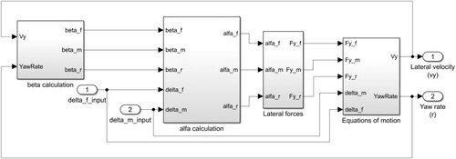24) for the forward problem of a 6x6 vehicle, Simulink® was used to model and simulate the vehicle behaviour using a block-diagram language given in Figure 14, while the parameters values were initialized using MATLAB®. The model was constructed based on algorithm 1.

Figure 14. Simulink® block-diagram.

4. Inverse problem analysis

4.1. Levenberg–Marquardt algorithm

As already mentioned, an inverse problem is the result of a process in which the mathematical model of a system and its output are known. However, some of the parameters used on the mathematical formulation are unknown and need to be estimated so that, when applied in the forward problem, can represent the process according to the real measurements. As stated by Lourakis et al. [38], the LM method is regarded as a standard technique for nonlinear least-squares problems, applied in several scientific areas. This algorithm is considered as a combination between steepest descent and Gauss–Newton method due to its behaviour: slow, but the convergence is assured when the algorithm is distant from the target, accordingly to the steepest descent method; while if close to the solution, it assumes a Gauss–Newton method.

The LM method consists of parameters estimation through an interactive process using the maximum-likelihood objective function [46,47] presented in Equation (33(33) $S_{\mathrm{M}\mathrm{L}}\left(\mathit{P}\right)=[\mathit{Y}-\stackrel{\mathbf{ˆ}}{\mathit{Y}}\mathbf{\left(}\mathit{P}\mathbf{\right)}{]}^{\mathrm{T}}W[\mathit{Y}-\stackrel{\mathbf{ˆ}}{\mathit{Y}}\mathbf{\left(}\mathit{P}\mathbf{\right)}],$(33) ): (33) $S_{\mathrm{M}\mathrm{L}}\left(\mathit{P}\right)=[\mathit{Y}-\stackrel{\mathbf{ˆ}}{\mathit{Y}}\mathbf{\left(}\mathit{P}\mathbf{\right)}{]}^{\mathrm{T}}W[\mathit{Y}-\stackrel{\mathbf{ˆ}}{\mathit{Y}}\mathbf{\left(}\mathit{P}\mathbf{\right)}],$(33) where P is the vector of unknown variables, Y is the vector containing the experimental measurements, Ŷ(P) is the solution of the forward problem applying the estimated parameters, the superscript T indicates the transpose of the vector, and W is a diagonal weighting matrix, which corresponds to the inverse of the covariance matrix of the measurements errors. Therefore, assuming that the measurements are uncorrelated, W is given by: (34) $W=\left(\begin{array}{cccc}1/{{\sigma }_1}^2& 0& \dots & 0\\ 0& 1/{{\sigma }_2}^2& \dots & 0\\ ⋮& ⋮& \dots & 0\\ 0& 0& \dots & 1/{{\sigma }_I}^2\end{array}\right),$(34) where I is the number of measurements and σ² is the variance associated with each measure. Since inverse parameters estimation problems can be very ill-conditioned, the recurrence equation, at each iteration k, applied using the LM Method, which attenuates this situation, is given by Equation (35(35) ${\mathit{P}}^{\mathbf{k}\mathbf{+}\mathbf{1}}={\mathit{P}}^{\mathbf{k}}+\left[\right(J^{\mathrm{k}}{)}^{\mathrm{T}}W{J}^{\mathrm{k}}+{\lambda }^{\mathrm{k}}{\mathrm{\Omega }}^{\mathrm{k}}{]}^{-1}\left(J^{\mathrm{k}}{)}^{\mathrm{T}}W\right[\mathit{Y}-\stackrel{\mathbf{ˆ}}{\mathit{Y}}\mathbf{\left(}{\mathit{P}}^{\mathbf{k}}\mathbf{\right)}],$(35) ) [47]: (35) ${\mathit{P}}^{\mathbf{k}\mathbf{+}\mathbf{1}}={\mathit{P}}^{\mathbf{k}}+\left[\right(J^{\mathrm{k}}{)}^{\mathrm{T}}W{J}^{\mathrm{k}}+{\lambda }^{\mathrm{k}}{\mathrm{\Omega }}^{\mathrm{k}}{]}^{-1}\left(J^{\mathrm{k}}{)}^{\mathrm{T}}W\right[\mathit{Y}-\stackrel{\mathbf{ˆ}}{\mathit{Y}}\mathbf{\left(}{\mathit{P}}^{\mathbf{k}}\mathbf{\right)}],$(35) where J is the sensitivity matrix defined by Equation (36(36) $\begin{array}{rl}J& =[\frac{\mathrm{\partial }{\stackrel{\mathbf{ˆ}}{\mathit{Y}}}^{\mathbf{T}}\mathbf{\left(}\mathit{P}\mathbf{\right)}}{\mathrm{\partial }\mathit{P}}{]}^{\mathrm{T}},\end{array}$(36) ) [47–49], λ is a scalar known as damping parameter, and Ω is a diagonal matrix [46,47,50] that can be expressed by Equation (37(37) $\begin{array}{rl}{\mathrm{\Omega }}^{\mathrm{k}}& =\mathrm{d}\mathrm{i}\mathrm{a}\mathrm{g}\left[\right(J^{\mathrm{k}}{)}^{\mathrm{T}}W{J}^{\mathrm{k}}].\end{array}$(37) ): (36) $\begin{array}{rl}J& =[\frac{\mathrm{\partial }{\stackrel{\mathbf{ˆ}}{\mathit{Y}}}^{\mathbf{T}}\mathbf{\left(}\mathit{P}\mathbf{\right)}}{\mathrm{\partial }\mathit{P}}{]}^{\mathrm{T}},\end{array}$(36) (37) $\begin{array}{rl}{\mathrm{\Omega }}^{\mathrm{k}}& =\mathrm{d}\mathrm{i}\mathrm{a}\mathrm{g}\left[\right(J^{\mathrm{k}}{)}^{\mathrm{T}}W{J}^{\mathrm{k}}].\end{array}$(37) It is important to highlight that problems satisfying $|J^{\mathrm{T}}J|\approx 0$ are ill-conditioned [50], where $|.|$ denotes the determinant of a matrix. Therefore, both λ and Ω are combined to damp oscillations and instabilities during the numerical solution of an inverse problem due to its ill-conditioned aspect by making the term λ^kΩ larger when compared to J^TWJ if needed [47]. Also, according to [38], the damping term contributes to accelerate the convergence process, and it is also important in situations where the Jacobian matrix is rank deficient. The LM algorithm is considered a simple, powerful and direct interactive method, capable of dealing with complex physical situations. Some usual stop criteria applied are: (38) $\begin{array}{r}\mathit{S}\left({\mathit{P}}^{\mathrm{k}+1}\right)<{ϵ}_1,\end{array}$(38) (39) $\begin{array}{r}||\left(J^{\mathrm{k}}{)}^{\mathrm{T}}\right[\mathit{Y}-\stackrel{\mathbf{ˆ}}{\mathit{Y}}\mathbf{\left(}{\mathit{P}}^{\mathbf{k}}\mathbf{\right)}]|{|}_{\mathrm{\infty }}<{ϵ}_2,\end{array}$(39) (40) $\begin{array}{r}||{\mathit{P}}^{\mathrm{k}+1}-{\mathit{P}}^{\mathrm{k}}|{|}_{\mathrm{\infty }}<{ϵ}_3.\end{array}$(40) where ε₁, ε₂ and ε₃ are tolerances, and $||.|{|}_{\mathrm{\infty }}$ is the infinite norm of the vector. The interactive method is outlined in Algorithm 2 for the cornering stiffness parameters estimation.

4.2. Sensitivity analysis

It is of great importance that the system output is sensible to the parameters, otherwise changes in their values will not present a significant variation on system output, preventing their estimation. Therefore, before LM approach application for the cornering stiffness estimation (Algorithm 2), a sensitivity analysis for each parameter C_αf, C_αm and C_αr was performed to verify their influence on the numerical solution for yaw rate measurements of the vehicle.

The analysis consisted on evaluating the reduced sensitivity coefficient X_r, calculated by taking the first derivative of a dependent variable with respect to a parameter multiplied by it [48]. Therefore, it expresses the variation of the response of a mathematical model output given changes in parameters values. Initially, it was considered a semi-sinusoidal trajectory (corresponding to a single-lane change) using the vehicle's parameters and the dimensions of the proposed standard in [39] during a 16 seconds manoeuvre for the steer angle δ_f calculation (a period of a sine function). This was used as an input for the mathematical model. The simulated measurements contained random errors applied on the forward problem yaw rate response with standard deviation σ = 0.0137°/s, based on the resolution of the sensor according to [41].

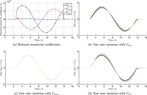
From the analysis of the reduced sensitivity coefficients along time illustrated in Figure 15(a), it is possible to conclude that C_αm effects over the yaw rate response are negligible compared to the other parameters, since changes in the associated reduced sensitivity coefficient X_rCαm are almost none. In order to confirm this statement, it was verified the yaw rate variation for different values of C_αf, C_αm and C_αr individually, as illustrated in Figures 15(a), 15(b) and 15(c), respectively. The C_α values ranged from 10,000 N rad⁻¹ to 400,000 N rad⁻¹, with a 10,000 N rad⁻¹ step. Isolated increments on C_αf resulted in higher values for the yaw rate, while the same performed on C_αr resulted in a lower response. From Figure 15(c), it is not possible to estimate C_αm. Therefore, the focus of this study was the estimation of the cornering stiffness parameters for the other axles, C_αf and C_αr, considering a constant and fixed value for C_αm.

Figure 15. Sensitivity analysis of the parameters with simulated measurements.

5. Results and discussion

Before using real data for the inverse analysis problem, two test problems were proposed to verify the algorithm applicability, robustness and efficiency to estimate the cornering stiffness. Firstly, simulated measurements were generated through computational implementation of the forward problem of the 6x6 vehicle using Simulink® and MATLAB®. Given that the objective was accomplished successfully, the next evaluation consisted in the estimation of those parameters using measurements gathered from Carsim^TM, which is a vehicle dynamics simulation software from Mechanical Simulation Corporation. Carsim^TM is well known for its accuracy and detailed simulations response of passengers cars used in the automotive industry, universities and research labs for studies and even validations of vehicle's performance. Many information of vehicles used for simulation on this software are available in its database, such as tyre's lateral force vs. slip angle, and vehicle's parameters. Considering that systems' non-linearity and environment disturbances (e.g. road roughness) are modelled in this software, it is indeed a more realistic measurement of a vehicle's real behaviour before the final estimation of the 6x6 cornering stiffness parameters using experimental data.

5.1. Estimation using simulated measurements of the 6x6 vehicle

Simulated measurements were generated through computational implementation of the forward problem of the 6x6 vehicle using Simulink® and MATLAB®. The front steer angle δ_f and the simulated measurements applied were the same used for the sensitivity analysis. Based on the study presented in [51] regarding the analysis of the cornering stiffness of a 14.00R20 tyre with run-flat insert, given a 500 kPa tyre pressure and an expected 2,667 kg tyre vertical load, it was assumed C_α ≈ 150,000 N rad⁻¹ for a single wheel.

Therefore, since the tyres cornering stiffness for the specific test vehicle were not available, it was assumed a fixed C_αm = 300,000 N rad⁻¹ from the assumption of equivalence of the parameter cornering stiffness for tyres in the same axle and subsequent application of Equations (15(15) $\begin{array}{rl}{C}_{{\alpha }_f}& =C_{{\alpha }_{f_L}}+C_{{\alpha }_{f_R}},\end{array}$(15) ) and (16(16) $\begin{array}{rl}{C}_{{\alpha }_r}& =C_{{\alpha }_{r_L}}+C_{{\alpha }_{r_R}},\end{array}$(16) ). For simulation measurements, the exact values of C_αf and C_αr were 400,000 N rad⁻¹ and 200,000 N rad⁻¹, respectively. The input variables to run the simulation are summarized in Table 3. The initial λ and the differential step were tuned for better running time performance.

Table 3. Parameters for simulated measurements application for a single-lane change manoeuvre.

MATLAB® inputs
Vehicle velocity	10 km h^−1
$C_{{\alpha }_{f}exact}$	400,000 N rad^−1
$C_{{\alpha }_{m}exact}$	300,000 N rad^−1
$C_{{\alpha }_{r}exact}$	200,000 N rad^−1
Differential step	10^−8
Initial λ	10^7
Error tolerance	10^−6
Maximum iteration	1000
Initial $C_{{\alpha }_f}$	100,000 N rad^−1
Initial $C_{{\alpha }_r}$	600,000 N rad^−1
Simulink® configuration
Solver	ode45, variable step
Solver maximum step size	10^−3
Relative tolerance	10^−6
Absolute tolerance	10^−6

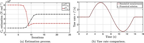
The LM method was successfully applied to estimate C_αf and C_αr values as can be seen in Figure 16(a), which expresses the estimation process at each iteration. Figure 16(b) illustrates the comparative response between the yaw rate simulated measurements and the numerical solution of the forward problem using the estimated parameters.

Figure 16. Estimation using simulated measurements during a single-lane change manoeuvre.

As an additional estimation, it was proposed the application of a step input in the SHM, which is usually applied to evaluate the behaviour of a dynamic system. According to [12], it is equivalent to a sudden change in the steer angle from zero to a nonzero constant value for vehicle dynamics. Therefore, supposing a sudden change in the front left wheel steer angle from 0 rad to 0.1 rad ≈5.73°, a simulation applying other values presented in Table 4 was also performed. The estimation process is illustrated in Figure 17(a), and the resultant comparative yaw rate response is presented in Figure 17(b).

Figure 17. Estimation using simulated measurements given a sudden steer change.

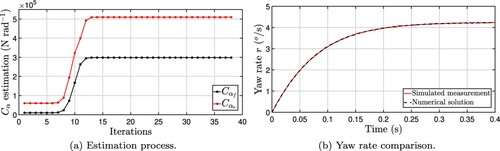
Table 4. Parameters for simulated measurements application for a sudden change in steer angle manoeuvre.

MATLAB® inputs
Vehicle velocity	10 km h^−1
δf	$\left\{\begin{array}{ll}0.1\mathrm{r}\mathrm{a}\mathrm{d},& t>0\\ \phantom{0.}0\mathrm{r}\mathrm{a}\mathrm{d},& t⩽0\end{array}\right.$
Cαfexact	300,000 N rad^−1
Cαmexact	400,000 N rad^−1
Cαrexact	500,000 N rad^−1
Differential step	10^−8
Initial λ	10^7
Error tolerance	10^−6
Maximum iteration	1000
Initial Cαf	10,000 N rad^−1
Initial Cαr	60,000 N rad^−1

Results for simulated measurements application for a single-lane change and for a sudden change in steer angle manoeuvres are summarized in Table 5, which exposes the LM algorithm effectiveness given the small relative errors associated with the estimated parameters. It is relevant to reaffirm that the simulated measurements contained random errors in order to include the measurements uncertainties, which are expected for real measurements data. According to Figures 16(b) and 17(b), the model with the estimated parameters satisfactorily represents the expected response.

Table 5. Estimation results for simulated measurements.

Parameter	Exact value	Estimated value^a	Relative error
	Single-lane change manoeuvre
Cαf	400,000 N rad^−1	400,365 N rad^−1	0.09%
Cαr	200,000 N rad^−1	199,848 N rad^−1	−0.08%
	Sudden change in steer angle manoeuvre
Cαf	300,000 N rad^−1	298,427 N rad^−1	−0.5%
Cαr	500,000 N rad^−1	509,801 N rad^−1	2.0%

Note: ${}^a$ Values rounded to the nearest integer.

5.2. Parameters estimation using carsim^TM measurements

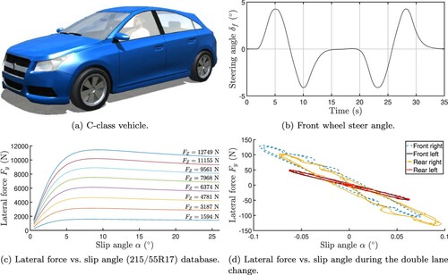
Carsim^TM is a simulation software for passenger vehicles and light-duty trucks, considered very detailed and accurate to represent a vehicle actual behaviour. Due to its widely application in automotive researches, including validation for dynamics mathematical models, a prior estimation of the cornering stiffness of the front and rear axle of a C-class vehicle included in this software database was performed.

Figures 18(a) and 18(b) show the mentioned vehicle and the front wheel steering angle extracted from Carsim^TM simulation, which is applied as an input to the SHM model of a two-axle vehicle during a double-lane change manoeuvre at 10 km h⁻¹. The lateral forces database for the 215/55R17 tyre used in this model is presented in Figure 18(c), showing that they varied according to the vertical load and the slip angle. In agreement with [25], it can be visualized in Figure 18(d) the phase lag between the slip angles and lateral forces in each tyre, attributed to the its relaxation length, that difficult the direct identification of the cornering stiffness.

Figure 18. Information extracted from Carsim^TM.

Simulation parameters used in the estimation process are presented in Table 6. Figure 19 shows the estimation process and the comparative yaw rate values, while Table 7 presents the estimated cornering stiffness values. The numerical solution is considered satisfactory to represent the yaw rate measurement given the root-mean-square error (RMSE) and multiple correlation coefficient ($R^2$ ) values (greater than 0.9).

Figure 19. Estimation results using Carsim^TM data of a double-lane change manoeuvre.

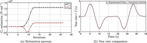
Table 6. Carsim^TM parameters used in the simulation of a single-lane change manoeuvre at 10 km h⁻¹.

MATLAB® inputs
Vehicle velocity	10 km h^−1
Vehicle mass m	1,501 kg
Yaw moment of inertia Iz	1,536.7 kg m^2
Front axle distance to CG	1.015 m
Rear axle distance to CG	1.895 m
Differential step	10^−8
Initial λ	10^6
Error tolerance	10^−6
Maximum iteration	1000
Initial Cαf	80,000 N rad^−1
Initial Cαr	80,000 N rad^−1

Table 7. Results with Carsim^TM measurements.

Parameter	Estimated value^(a)	Yaw rate RMSE^(b)	R^2(c)
Cαf	144,307N  rad^−1	0.04°/s	0.9997
Cαr	92,498 N rad^1

Note: ^aValues rounded to the nearest integer.

^bRoot-mean-square error between the experimental data and the numerical solution.

^cMultiple correlation coefficient.

In order to compare the estimated parameters values with one of the commonly applied technique mentioned in Section 1, a Forgetting-factor Recursive Least Squares (FF-RLS) was applied to identify the time-varying cornering stiffness parameters. Since that the lateral forces and slip angles are available for each tyre, this comparison is simplified because the estimation of those states are not necessary. Therefore, the FF-RLS formulation consists in representing the system as a linear regression model, such that: (41) $y\left(t\right)=\phi \left(t\right)\hat{\theta }\left(t\right)+{\xi }_i\left(t\right)\to F_{y_i}\left(t\right)=-{\alpha }_i\left(t\right){\hat{C}}_{{\alpha }_i}\left(t\right)+{\xi }_i\left(t\right),$(41) where F_yi denotes the system output y on the wheel i, while −α_i is the input (φ), Ĉ_αi is the instantaneous identified parameters ($\hat{\theta }$) and ξ_i is the difference of the measured and predicted output (residuals). The recursive FF-RLS is described by Equation 42(42) $\begin{array}{rl}{P}_k& =\frac{1}{\lambda }(I-K_k{\phi }_k^{\mathrm{T}})P_{k-1},\end{array}$(42) , 43(43) $\begin{array}{rl}{K}_k& =\frac{P_{k-1}{\phi }_k}{\lambda +{\phi }_k^{\mathrm{T}}{P}_{k-1}{\phi }_k},\end{array}$(43) and 44(44) $\begin{array}{rl}{\hat{\theta }}_k& ={\hat{\theta }}_{k-1}+K_k(y_k-{\phi }_k^{\mathrm{T}}{\hat{\theta }}_{k-1}),\end{array}$(44) [52]: (42) $\begin{array}{rl}{P}_k& =\frac{1}{\lambda }(I-K_k{\phi }_k^{\mathrm{T}})P_{k-1},\end{array}$(42) (43) $\begin{array}{rl}{K}_k& =\frac{P_{k-1}{\phi }_k}{\lambda +{\phi }_k^{\mathrm{T}}{P}_{k-1}{\phi }_k},\end{array}$(43) (44) $\begin{array}{rl}{\hat{\theta }}_k& ={\hat{\theta }}_{k-1}+K_k(y_k-{\phi }_k^{\mathrm{T}}{\hat{\theta }}_{k-1}),\end{array}$(44) where K is the estimator gain, P is the covariance and λ is the forgetting factor. Basically, the FF-RLS algorithm consists in initializing P(0) and $\hat{\theta }\left(0\right)$, and perform iteratively:

1. Measure the current input/output of the system: y(k), u(k);

2. Calculate the prediction error $\xi \left(k\right)=y\left(k\right)-\phi (k{)}^{\mathrm{T}}\hat{\theta }(k-1)$;

3. Calculate the estimator gain using Equation  (44(44) $\begin{array}{rl}{\hat{\theta }}_k& ={\hat{\theta }}_{k-1}+K_k(y_k-{\phi }_k^{\mathrm{T}}{\hat{\theta }}_{k-1}),\end{array}$(44) );

4. Calculate the covariance applying Equation  (42(42) $\begin{array}{rl}{P}_k& =\frac{1}{\lambda }(I-K_k{\phi }_k^{\mathrm{T}})P_{k-1},\end{array}$(42) );

5. Update estimated parameters using Equation  (44(44) $\begin{array}{rl}{\hat{\theta }}_k& ={\hat{\theta }}_{k-1}+K_k(y_k-{\phi }_k^{\mathrm{T}}{\hat{\theta }}_{k-1}),\end{array}$(44) ).

The simulation parameters applied in the FF-RLS method for each tyre were P(0) = 10⁵, $\hat{\theta }\left(0\right)=40,000$ and λ = 0.999. Figures 20 and 21 show the results using this method.

Figure 20. Measured and predicted lateral force on each tyre applying FF-RLS.

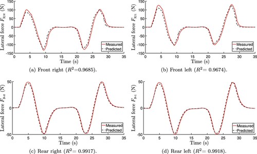
Figure 21. Estimated parameters using FF-RLS.

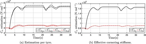
According to Figure 20, the predicted lateral forces present a good agreement with the measurements, since R² > 0.9. Figures 21(a) and 21(b) show the identified parameters along the manoeuvre time for each tyre and the effective cornering stiffness per axle, respectively. As can be seen in Figure 21(b), when the lateral forces varied, starting at 2 seconds of simulation, the effective front cornering stiffness varied in the interval [75,894:167,790] N rad⁻¹, assuming a final value of 165,380 N rad⁻¹, while the effective rear cornering stiffness varied in the interval [76,188:90,263] N rad⁻¹, assuming a final value of 90,263 N rad⁻¹. Compared to the results using the LM approach presented in Table 7, the differences of the estimated parameters using the LM approach was −12.7% and 2.5% for the front and rear axle, respectively, when compared to the final identified parameters using FF-RLS. It is highlighted that to perform the identification using the RLS directly, the slip angles and lateral forces on each tyre, two difficult measures in practice, were used, while only the yaw rate experimental values, more reliable measurements in practice, were applied using the LM estimation.

5.3. Results with real measurements

In this investigation, a mathematical model and real data measurements of the vehicle presented in Section 2 were used. In order to apply the LM algorithm with real measurements, it was necessary to provide the same steer angle on the front left wheel during the double-lane change manoeuvre. Since the angle of the driver's steering wheel was recorded in the log file of the test, and there was a linear function relation between the driver's steering wheel and the angle of the front left wheel steering ratio, it was possible to obtain the values needed. Also, it was necessary to establish the same simulation time and time step used in the log files.

Therefore, additional parameters were set in Simulink^® configuration, limiting data points to produce specified output only at time intervals from 0.00 s to 35.00 s (log file duration), at a 0.01 s time step. Adjustments presented in Table 8 were made in MATLAB^® inputs. Estimated cornering stiffness parameters at each iteration are presented in Figure 22(a). Applying the estimated parameters on the vehicle model, the yaw rate was calculated and the comparison between the experimental data and the numerical solution is presented in Figure 22(b). The residual between the estimation and measurements is presented in Figure 22(c). Results are summarized in Table 9. The yaw rate RMSE and R² between the experimental measurements and the numerical solution of the forward problem were considered satisfactory.

Figure 22. Estimation results using experimental measurements of a double-lane change manoeuvre.

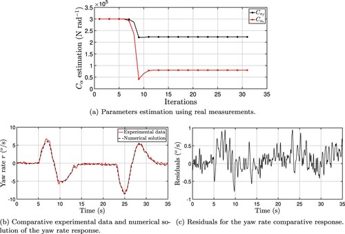
Table 8. Simulation parameters for real measurements application.

MATLAB^® inputs
$C_{{\alpha }_m\mathrm{f}\mathrm{i}\mathrm{x}\mathrm{e}\mathrm{d}}$	300,000 N rad^−1
Differential step	10^−8
Initial λ	10^7
Error tolerance	10^−6
Maximum iteration	1000
Initial $C_{{\alpha }_f}$	300,000 N rad^−1
Initial $C_{{\alpha }_r}$	300,000 N rad^−1

Table 9. Results with experimental measurements.

Parameter	Estimated value^a	Yaw rate RMSE^b	R^2c
$\begin{array}{l}{C}_{{\alpha }_f}\\ C_{{\alpha }_r}\end{array}$	$\begin{array}{c}222,930\phantom{}{\mathrm{N}\mathrm{r}\mathrm{a}\mathrm{d}}^{-1}\\ \phantom{2}80,032\phantom{}{\mathrm{N}\mathrm{r}\mathrm{a}\mathrm{d}}^{-1}\end{array}$	0.30°/s	0.9906

Note: ^aValues rounded to the nearest integer.

^bRoot-mean-square error between the experimental data and the numerical solution.

^cMultiple correlation coefficient.

From the results presented, there is a good agreement between the yaw rate experimental measurements and the numerical solution obtained using the estimated parameters. Also, according to the vehicle's assessment report, the loaded is distributed between axles in the following manner: the middle and front axles hold the higher normal load, 38% and 36 %, respectively, while the rear axle is responsible for 26% of the total vertical load on the vehicle, considering the test condition, which corresponds to the expected values obtained for the cornering stiffness being higher for the front and middle axles. It is important to highlight that sensor calibration and its position show a considerable influence on the measurements data, which interferes in related studies. Therefore, adjustments mentioned in Section 2 were fundamental in order to obtained the satisfactory results.

6. Conclusion

This study presented an integration between a mathematical vehicle model and real data measurements in order to estimate cornering stiffness, which is a critical parameter for vehicle lateral dynamics analysis, especially its stability. A two degree-of-freedom 6x6 wheeled vehicle model was established for cornering stiffness parameters estimation, since they are not usually provided by the tyre's manufacturer and their measurement requires specific vehicle's instrumentation, structure and time availability.

The mathematical formulation proposed a simple handling model (SHM), also known as bicycle model, to represent the lateral dynamics of a 6 × 6 vehicle, assuming small steering angles at low velocities manoeuvres. The LM approach was based on the numerical solution of the forward problem given by the proposed model and yaw rate measurements collected from field experiments of a vehicle during double-lane change manoeuvres. The simulated yaw rate response applying the estimated cornering stiffness parameters in the SHM presents a similar behaviour when compared to real experiments data, even though a relatively simple model was applied.

For this reason, it is worth highlighting the importance of the study and application of a inverse problem analysis as well as techniques for the estimation of unknown parameters, usually difficult or impossible to measure accurately. Given all inputs available for a computational vehicle model, it is possible to predict some of the vehicle dynamics characteristics, and even point out modification on a vehicle project to enhance its performance prior to its manufacturing, such as stability and steering. Besides that, lateral dynamics models are also highly applied for vehicle control strategies, which enable development of semi and autonomous vehicles. Since the cornering stiffness parameters are usually applied in control system strategies, such as electronic stability control (ESC), and also used on formulation to estimate others vehicles states and parameters, future studies are focused on verify the algorithm application in real-time and the design of a model predictive control (MPC) approach in order to incorporate advanced control system in the vehicle.

Nomenclature

α	=	Slip angle
β	=	Sideslip angle or attitude angle
δ	=	Steer angle of a tyre
ωy	=	Angular velocity of the vehicle in the y-axis
ωx	=	Angular velocity of the vehicle in the x-axis
ωz	=	Angular velocity of the vehicle in the z-axis
ψ	=	Yaw angle or heading angle
θ	=	Pitch angle
φ	=	Roll angle
a1	=	Distance of the front wheel to the centre of mass of a vehicle
a2	=	Distance of the second wheel to the centre of mass of a vehicle
a3	=	Distance of the third wheel to the centre of mass of a vehicle
ay	=	Lateral acceleration
Cα	=	Cornering stiffness
Fx	=	Longitudinal force on a vehicle
Fy	=	Lateral force on a vehicle
Fxi	=	Longitudinal tyre force
Fyi	=	tyre lateral force
g	=	Gravitational acceleration
H	=	Maximum height of the vehicle
Iz	=	Moment of inertia of a vehicle along z-axis
L	=	Total length of the vehicle
l	=	Wheelbase of the vehicle
Mz	=	Yaw Moment
m	=	Total mass of the vehicle
p	=	Roll rate of a vehicle
Ptyre	=	tyre inflation pressure
q	=	Pitch rate of a vehicle
r	=	Yaw rate of a vehicle
vy	=	Lateral velocity of a vehicle
vx	=	Longitudinal velocity of a vehicle
wv	=	Maximum width of the vehicle
w	=	Track of the vehicle

Acknowledgments

The authors would like to thank Mr. Madson Ferrari Pereira, Head of LATAM Product Validation at IVECO Latin America, for providing technical support during the field experimental measurements, and the Brazilian Army for supporting research and scientific development in military equipment.

Disclosure statement

No potential conflict of interest was reported by the author(s).

References

- Jin X, Yin G, Chen N. Advanced estimation techniques for vehicle system dynamic state: A survey. Sensors. 2019;19(19):4289.
- Viehweger M, Vaseur C, van Aalst S, et al. Vehicle state and tyre force estimation: demonstrations and guidelines. Vehicle Syst Dyn. 2020;59(5):675–702.
- Cuma MU, Koroglu T. A comprehensive review on estimation strategies used in hybrid and battery electric vehicles. Renewable and Sustainable Energy Reviews. 2015;42:517–531.
- Wang Y, Geng K, Xu L, et al. Estimation of sideslip angle and tire cornering stiffness using fuzzy adaptive robust cubature kalman filter. IEEE Trans Syst Man Cybern: Syst. 2020: 1–12.
- Alatorre AG, Charara A, Victorino A, et al. Sideslip estimation algorithm comparison between euler angles and quaternion approaches with black box vehicle model. In: 2018 IEEE 15th Int Workshop Adv Motion Control (AMC); IEEE. 2020;553–559. https://ieeexplore.ieee.org/document/8371153.
- Liu Y, Ji X, Yang K, et al. Finite-time optimized robust control with adaptive state estimation algorithm for autonomous heavy vehicle. Mech Syst Signal Process. 2020;139:106616.
- Ni J, Hu J, Xiang C. A review for design and dynamics control of unmanned ground vehicle. Proc Institution Mech Eng Part D: J Automobile Eng.2021;235(4):1084–1100.
- Acosta M, Kanarachos S. Tire lateral force estimation and grip potential identification using neural networks, extended kalman filter, and recursive least squares. Neural Comput Appl. 2018;30(11):3445–3465.
- Melzi S, Sabbioni E. On the vehicle sideslip angle estimation through neural networks: numerical and experimental results. Mech Syst Signal Process. 2011;25(6):2005–2019.
- Van Eeden CJ, et al. The steering relationship between the first and second axles of a 6x6 off-road military vehicle [dissertation]. University of Pretoria; 2007.
- Baffet G, Charara A, Lechner D. Estimation of vehicle sideslip, tire force and wheel cornering stiffness. Control Eng Pract. 2009;17(11):1255–1264.
- Jazar RN. Vehicle planar dynamics. In: Vehicle dynamics: Theory and application. Springer; 2008. p. 583–659.
- Arndt M, Ding E, Massel T. Identification of cornering stiffness during lane change maneuvers. In: Proc 2004 IEEE Int Conf Control Appl. 2004;1:344–349.IEEE; 2004.
- Xu S, Peng H. Design, analysis, and experiments of preview path tracking control for autonomous vehicles. IEEE Trans Intell Transp Syst. 2019;21(1):48–58.
- Hu C, Wang Z, Qin Y, et al. Lane keeping control of autonomous vehicles with prescribed performance considering the rollover prevention and input saturation. IEEE Trans Intell Transp Syst. 2020;21(7):3091–3103.
- Lin F, Wang S, Zhao Y, et al. Research on autonomous vehicle path tracking control considering roll stability. Proc Institution Mech Eng Part D: J Automobile Eng. 2021;235(1):199–210.
- Ataei M, Khajepour A, Jeon S. Model predictive rollover prevention for steer-by-wire vehicles with a new rollover index. Int J Control. 2020;93(1):140–155.
- Ataei M, Khajepour A, Jeon S. Model predictive control for integrated lateral stability, traction/braking control, and rollover prevention of electric vehicles. Vehicle Syst Dyn. 2020;58(1):49–73.
- Cui Q, Ding R, Wei C, et al. Path-tracking and lateral stabilisation for autonomous vehicles by using the steering angle envelope. Vehicle System Dynamics. 2020;1–25. https://www.tandfonline.com/doi/citedby/https://doi.org/10.1080/00423114.2020.1776344?scroll=top&needAccess=true.
- Forte L, et al. Low-cost method of estimating vehicle sideslip and tire cornering stiffness using global positioning and inertial measurement [dissertation]. State University of New York at Buffalo; 2019.
- Feng L, Chen W, Wu T, et al. An improved sensor system for wheel force detection with motion-force decoupling technique. Meas. 2018;119:205–217.
- Aliganov OM. Inverse problems in the design, modeling and testing of engineering systems. Third International Conference on Inverse Design Concepts and Optimization in Engineering Sciences (ICIDES-3); Oct 1991; Washington, DC. p. 495–512.
- An SJ, Yi K, Jung G, et al. Desired yaw rate and steering control method during cornering for a six-wheeled vehicle. Int J Automot Technol. 2008;9(2):173–181.
- O'Brien R, Kiriakidis K. A comparison of h/spl infin/with kalman filtering in vehicle state and parameter identification. In: 2006 Am Control Conf IEEE. 2006;3954–3959. https://ieeexplore.ieee.org/document/1657336.
- Sierra C, Tseng E, Jain A, et al. Cornering stiffness estimation based on vehicle lateral dynamics. Vehicle Syst Dyn. 2006;44(sup1):24–38.
- Davoodabadi I, Ramezani AA, Mahmoodi-k M, et al. Identification of tire forces using dual unscented kalman filter algorithm. Nonlinear Dyn. 2014;78(3):1907–1919.
- Lee S, Nakano K, Ohori M. On-board identification of tyre cornering stiffness using dual kalman filter and gps. Vehicle Syst Dyn. 2015;53(4):437–448.
- Bechtoff J, Isermann R. Cornering stiffness and sideslip angle estimation for integrated vehicle dynamics control. IFAC-PapersOnLine. 2016;49(11):297–304.
- Di Biase F, Lenzo B, Timpone F. Vehicle sideslip angle estimation for a heavy-duty vehicle via extended kalman filter using a rational tyre model. IEEE Access. 2020;8:142120–142130.
- Lundquist C, Schön TB. Recursive identification of cornering stiffness parameters for an enhanced single track model. IFAC Proc Volumes. 2009;42(10):1726–1731.
- Nam K, Fujimoto H, Hori Y. Lateral stability control of in-wheel-motor-driven electric vehicles based on sideslip angle estimation using lateral tire force sensors. IEEE Trans Vehicular Technol. 2012;61(5):1972–1985.
- Singh KB, Arat MA, Taheri S. Literature review and fundamental approaches for vehicle and tire state estimation. Vehicle Syst Dyn. 2019;57(11):1643–1665.
- Lopes A, Araújo RE. Vehicle lateral dynamic identification method based on adaptive algorithm. IEEE Open J Vehicular Technol. 2020;1:267–278.
- Ghandour R, Victorino A, Doumiati M, et al. Tire/road friction coefficient estimation applied to road safety. In: 18th Mediterr Conf Control Autom, MED'10; IEEE. 2010;1485–1490. https://ieeexplore.ieee.org/document/5547840.
- Ghandour R, Victorino A, Charara A, et al. A vehicle skid indicator based on maximum friction estimation. IFAC Proc Volumes. 2011;44(1):2272–2277.
- El Hajjaji A, Chadli M, Oudghiri M, et al. Observer-based robust fuzzy control for vehicle lateral dynamics. In: 2006 Am Control Conf IEEE. 2006;4664–4669. https://ieeexplore.ieee.org/document/1657457.
- Yu H, Wilamowski BM. Levenberg-marquardt training. Ind Electron Handb. 2011;5(12):1.
- Lourakis MI, et al. A brief description of the levenberg-marquardt algorithm implemented by levmar. Found Res Technol. 2005;4(1):1–6.
- North Atlantic Treaty Organization (NATO). NATO Dynamic Stability, AVTP 03-160 W; September 1991. p. 665–725.
- Gunter DD, Bylsma WW, Edgar K, et al. Using modeling and simulation to evaluate stability and traction performance of a track-laying robotic vehicle. In: Enabling Technol Simul Sci IX. 2005;5805:66–73.International Society for Optics and Photonics.
- Racelogic. IMU03 and YAW03 Inertial Sensor User Guide; December 11, 2014. Version 1.
- Nirmal K, Sreejith A, Mathew J, et al. Noise modeling and analysis of an imu-based attitude sensor: improvement of performance by filtering and sensor fusion. In: Advances in Optical and Mechanical Technologies for Telescopes and Instrumentation II. 2016;9912:International Society for Optics and Photonics; 2016. p. 99126W.
- Gillespie TD. Fundamentals of vehicle dynamics. 400; Warrendale (PA): Society of Automotive Engineers; 1992.
- Vorotović GS, Rakicević BB, Mitić SR, et al. Determination of cornering stiffness through integration of a mathematical model and real vehicle exploitation parameters. FME Trans. 2013;41(1):66–71.
- Stéphant J, Charara A, Meizel D, et al. Evaluation of a sliding mode observer for vehicle sideslip angle. Control Eng Pract. 2007;15(7):803–812.
- Colaço MJ, Orlande HRB, Dulikravich GS, et al. Inverse and optimization problems in heat transfer. J Braz Soc Mech Sci Eng. 2006;28(1):1–24.
- Orlande HRB. Inverse problems in heat transfer: new trends on solution methodologies and applications.ASME. J. Heat Transfer. 2012;134(3):031011(1)–031011(13).
- Beck JV, Arnold KJ. Parameter estimation in engineering and science. New York: James Beck; 1977.
- Ozisik MN, Orlande HRB. Inverse heat transfer: fundamentals and applications. New York: Taylor and Francis; 2000.
- Grysa K. Inverse heat conduction problems. In: Vikhrenko VS, editor. Heat conduction. Chapter 1. Rijeka: IntechOpen; 2011. p. 20–22. https://doi.org/https://doi.org/10.5772/26575.
- Luty W, Simiński P. An analysis of cornering stiffness of 14.00 r20 tire with run-flat insert. J KONES. 2008;15:295–304.
- Tian Y, Lian Y, Tian C, et al. Sideslip angle and tire cornering stiffness estimations for four-in-wheel-motor-driven electric vehicles. In: 2019 Chin Control Conf (CCC) IEEE. 2019;2418–2423. https://ieeexplore.ieee.org/document/8866066.