Force-based stiffness mapping for early detection of breast cancer

ABSTRACT

Early detection of breast cancer will continue to be crucial in improving patient survival rates for the foreseeable future. Our long-term goal is to automate and refine the manual breast exam process using measured data on the breast surface in combination with formal inverse techniques to generate three-dimensional maps of the stiffness inside the breast tissue. In this paper, we report on computational techniques that use force measurements to create the stiffness map and validate the computational techniques experimentally with silicone tissue phantom experiments. We conducted 16 tests on tumour-free phantom samples and 16 tests on tumour-containing phantoms. Our stiffness mapping approach resulted in one false positive and a correct identification of the remaining 31/32 samples.

Keywords:

• Breast cancer
• genetic algorithm
• finite elements
• experimental validation
• parameter estimation

2010 Mathematics Subject Classification:

• 65N21

1. Introduction

Early detection of breast cancer is crucial for improving patient survival rates. Manual breast exams (breast palpation) and mammograms are currently the most effective and widely used early detection techniques. Manual breast exams depend on stiffness differences between healthy and cancerous tissues but are limited in their ability to detect tumours since they only produce local information about the site where the force is applied and do not provide quantitative measurements. Mammograms, while effective, expose the patient to radiation and hence routine mammograms are limited to those in specific age or risk groups. In addition, mammograms are sensitive to tissue density rather than tissue stiffness. While cancerous tissues are more dense than healthy tissues for many patients, for the roughly half of women over 40 with dense breasts [1] the differences are small and can be difficult to detect [1,2]. However, breast tumours are typically much stiffer than healthy tissue. Our goal is to develop a new method for the routine early detection of tumours which exploits this stiffness difference without exposing the patient to radiation.

It is widely agreed that cancerous tissue has an elastic modulus (stiffness) as much as 10 times that of the surrounding breast tissue [3,4]. Not only is this the basis of manual breast exams, but it is also the reason many researchers have studied approaches that use MRI, CT, or ultrasound measurements to create elastic modulus maps of the breast tissue. (Greenleaf et al. [4] provide a detailed review.) However, because they are expensive and stressful to the patient (particularly CT/MRI) these techniques primarily address the classification of cancerous sites in patients where suspected tumours have already been identified by other early detection methods.

Our long-term goal is to automate and refine the manual breast exam process using measured data on the breast surface in combination with formal inverse techniques to produce three-dimensional (3D) maps of the stiffness inside the breast tissue. We envision an electromechanical device that would gently indent the breast surface at multiple sites, and at each site the device would record the required indentation force and the displacements of the entire breast surface. Formal inverse techniques (finite element methods in combination with a genetic algorithm) would be used to find the stiffness (Young's modulus) distribution throughout the interior of the breast and create a visual 3D stiffness map for immediate use by the clinician. These stiffness maps could also be retained and compared with results from subsequent exams. Since this is envisioned as an early detection technique, we anticipate that suspicious sites would then be examined with established imaging modalities such as mammograms and ultrasound.

We are working towards this goal but it will take time to fully realize. This paper describes another essential advancement in the process.

We have previously developed appropriate computational algorithms for this stiffness mapping approach based on displacement measurements only and have examined their performance extensively on two- and three-dimensional model problems [5–7]. Over the past 2 years, we successfully validated the displacement-only approaches through gelatin tissue phantom experiments [8]. We tested 12 tumour-free samples and 14 tumour-containing samples and all cases were correctly identified. That work did not incorporate the force data.

In this paper, we examine the use of surface force data rather than surface displacement data. While definitely more intuitive than surface displacement data, the surface force data introduces new challenges. We present new methodologies for force-based tissue phantom experiments and key advances required for the computational algorithms. We successfully validate the computational algorithms with the tissue phantom experiments and identify the strengths and weaknesses of each measurement modality.

Section 2 discusses related work in this field, Section 3 describes the experimental procedures for the tissue phantom experiments, Section 4 reviews our computational approaches, Section 5 presents and discusses our results, and Section 6 summarizes our work and discusses future work.

2. Background literature

Existing studies on identifying stiffer cancerous tissues in otherwise healthy breast tissue fall into two broad categories – methods that require the displacement field (or strain field) within the breast tissue and methods that measure pressures/forces or displacements on the breast surface.

Methods that require the displacement field within the breast tissue

Greenleaf et al. [4], Doyley [9], Parker et al. [10], and Alam and Garra [11] provide reviews of the first class of techniques, which are referred to by a variety of names, including ‘elastography’, ‘elasticity imaging’, ‘elastic modulus imaging’, ‘ultrafast imaging’, and ‘vibroacoustography’. Each of these methods uses formal inverse techniques to infer the shear modulus or Young's modulus distribution in the breast tissue from measurements of the displacement or strain throughout the interior of the breast. The methods differ in the loading used to cause the displacements (external static loads, external time-dependent loads, or internal time-dependent loads), and the methods used to measure the displacements (typically ultrasound-based or magnetic resonance-based techniques). This first category of techniques has a rich history of contributions by many researchers. These methods all employ ultrasound, magnetic resonance, or computed tomography techniques to measure the displacements within the breast tissue, and they require relatively sophisticated equipment (and in some cases exposure to radiation). Li and Cao [12] review the technologies behind commercial ultrasound elastography systems and consensus guidelines for their use have been developed [13–16]. Much recent work has focused on non-invasively characterizing tissue pathology (especially by mapping nonlinear material properties) [14,17–22]. While these methods show promise for localizing already-identified tumours more accurately and non-invasively characterizing tissue pathology, they are unlikely to be used for routine screening of all patients in the near future.

Methods that measure pressures/forces or displacements on the breast surface

Studies related to ‘tactile imaging’ or ‘mechanical imaging’ [23–28] take a fundamentally different approach. Here a transducer (similar to an ultrasound wand) is manually scanned over the breast surface. The transducer measures reaction pressures, and the patterns overlap to form a full map of the reaction pressures. Sarvazyan et al. have further developed this approach and marketed it as the medical device ‘SureTouch’ [29–37]. Surface stress patterns are measured by a wand which is scanned over the surface of the breast. From this data, a semi-empirical approach is used to create a 3D image of the breast [35]. This device is now FDA-cleared as a Class II medical device and marketed for clinical use. The main audience for the device is women who refuse regular mammographic screening, women under 40 who seek screening, and women who have contraindications to radiation and severe breast compression [38].

Shih et al. have independently developed a manual surface-scanned transducer that currently marketed as the medical device ‘iBreastExam’ or iBE [39–44]. It has received FDA approval as a tool for documenting clinical findings in the breast. Conceptually, this is a ‘piezoelectric finger’– a flexible cantilever with attached force/displacement sensors which is scanned over the tissue surface. The results are mapped to a 1D equation to infer the tissue stiffness beneath the surface. Most recently [45] the commercialized product has been studied for use as a screening device with 486 patients who completed iBE, a clinical breast exam (CBE), and mammography. Of the 486 patients, 101 had positive iBE results, 12 of those had positive mammograms, and 3 ultimately were diagnosed with malignancies. CBE had 66 positive results, and again 12 of those had positive mammograms with 3 malignancies. Both iBE and CBE missed two small malignancies (3 mm and 1 cm) that were detected by mammography. They conclude that iBE performs comparably to the clinical breast exam as a triage tool.

Chase et al. developed a different approach termed Digital Imaging Elasto-Tomography or DIET [46–54]. They apply an external sinusoidal excitation to the breast surface and measure the steady-state motion of the tissue surface with digital cameras. Note that this introduces tissue density into the calculations in addition to the tissue stiffness. Their recent paper [46] gives an excellent overview of the approaches they have used to extract the stiffer locations from the dynamic tissue surface data. Initially [48,49] they explored methods that use finite element methods and formal inverse techniques to identify the stiffer regions, but they concluded that the computational effort and operator expertise levels were too high. Subsequently [55] they explored modal analysis but found that the inclusion size had a strong influence on the results and even 20 mm inclusions could not be detected reliably for some phantoms. In their work from 2018 [46] they examine a method that maps the point-wise local hysteresis loops to a simple (local) mass-spring model and extract nominal stiffnesses for each surface location. Regions with outliers in the nominal stiffness are identified as tumour locations. The process is fast computationally and could be automated for the four silicone phantoms tested (one tumour-free and three with tumours). Some limitations of the approach will still need to be addressed with additional testing/validation. The phantoms tested were all 53 mm high with all tumours placed 32 mm from the chest wall, and it appears that they were fairly close to the tissue surface. The region within 6 mm of the chest wall was excluded from the identification and the tissue slice 6 mm (height) from the excitation source was not observable. Additional testing will certainly aid in understanding whether the method can retain its identification abilities in more complicated situations.

As with our proposed technique, these methods use surface measurements. However, heuristic or approximate relationships are used to characterize the tumours rather than formal inverse techniques.

Goenezen et al. have introduced a method they refer to as ‘Mechanics Based Tomography’ [56–61]. This method is the most similar to ours in that it imposes surface forces and displacements to produce multiple displacement measurements on the domain boundary. These displacement measurements are used to estimate the material property distribution within the domain using finite elements and formal inverse techniques. However, their approach to the computational task of making the material property estimate is fundamentally different from our approach. They interpolate the material properties to the nodes of the finite element mesh and stabilize the solution with a total variation diminishing regularization on the material property distribution. While this gives a very broad set of possible material property distributions, the large relatively unconstrained solution space (35,000 unknown material properties in their most recent three-dimensional simulations [56]) may have consequences for the stability of the method. Measurements on a 7-cm cube with two cylindrical inclusions (1 cm and 1.4 cm radii) demonstrated the ability to recover the shear modulus of the smaller inclusion well but significantly overestimated the shear modulus of the larger inclusion. Nevertheless, under these conditions the method showed promise in that the inclusions could be imaged clearly even though the relative values of the modulus showed errors. It may be possible to stabilize the solutions with additional constraints.

In what follows, we seek to develop formal inverse techniques which infer (or map) the stiffness throughout the breast tissue based only on a knowledge of quasi-static surface forces, automating and refining techniques used in breast palpation. Our approach to the computational task of making the material property estimate uses a finite element model for the tissue along with a number of physically relevant constraints on the material property distribution. These constraints act to stabilize the solution in addition to an explicit regularization based on tumour size. Section 3 describes our methods in detail.

2.1. Material models and properties for breast tissues

As in our previous work on displacement-only stiffness mapping [8], we employ an incompressible linear elastic model in the computations along with small indentation depths to maintain linearity in the experiments.

The use of a linear elastic model for small strains in breast tissues is supported by many researchers [3,4,62–69]. Of particular interest is the work of Samani et al. [3,63] which included 169 tissue samples. Using a linear elastic model for the tissues, fat had a Young's modulus of 3.25±0.91 kPa, which was similar to healthy fibroglandular tissue at 3.24±0.61 kPa. In contrast, intermediate-grade IDC (Invasive Ductal Carcinoma) had a stiffness of 19.99±4.2 kPa and high-grade IDC was 42.52±12.47 kPa. They concluded that a linear elastic model was adequate for cancerous tissues. Barbone and Oberai's work on nonlinear material models for elastography is also of particular relevance here [67–69]. They conclude that the nonlinear term is a better discriminator of tumour type (benign or cancerous) but they also conclude that small strain results are essentially independent of the nonlinear term and that the tumours themselves rarely see large strains since they are embedded in substantially less stiff tissues. (A more detailed review may be found in our previous paper [8].)

Our experiments for this force-only research used silicone phantoms with a healthy tissue stiffness of approximately 3.2 kPa and a cancerous tissue stiffness of approximately 22.6 kPa. We again use an incompressible linear elastic model in our computations with those same stiffnesses. This is discussed in more detail in Section 3.

2.2. Breast volume

As in our previous work [8] our testing used a 180-g tissue phantom with a density very close to 1 g/cc, such that our phantom volumes were approximately 180 cc. Data on breast volume is quite limited. 180 cc corresponds to a value between the average and median breast volume from the work of Loughry et al. [70,71] who published some of the most extensive data available. They used biostereometric analysis to evaluate 598 randomly chosen women who received mammograms at Akron City Hospital and report an average breast volume of 203 cc with a median somewhat lower at approximately 170 cc. Note that our starting point of 180cc would represent a typical patient and additional sizes of tissue phantoms would need to be considered in future studies. (A more detailed review may be found in our previous paper [8].)

3. Experimental methods

3.1. Phantom creation

We created silicone phantoms with stiff tumour inclusions using materials examined by Kashif et al. [72]. The soft gel silicone¹ is mixed at a 10:1 base-to-catalyst ratio and diluted with silicone fluid² to further reduce the stiffness. We control the stiffness by adjusting the weight percentage of silicone fluid in the final mixture. At 66% silicone fluid, the Young's modulus was tested and found to be 3.2±0.4 kPa and that formulation was used to create healthy tissue. Appendix 2 gives details on the methods used to characterize the silicone modulus. Red coloring³ was added (0.2% by weight) to a 16% silicone fluid mixture to create tumours. The Young's modulus of that mixture was tested and found to be 22.6±1.5 kPa.

Tumour-free phantoms were prepared by mixing approximately 190 g of the 66% fluid mixture in a disposable polypropylene container, stirring constantly for 5 minutes. 180 g of the mixture was then immediately poured into a roughly hemispherical 120 mm diameter mould⁴ that been sprayed with mould release.⁵ The silicone/mould was immediately moved to a vacuum desiccator⁶ and degassed for 15 minutes. Then the vacuum was released and the silicone was allowed to cure in the mould at least overnight. (The nominal cure time for the soft gel silicone is 1 hour.) Phantoms were carefully removed from the mould and the surface was coated with talcum powder⁷ to prevent sticking. When not in use, phantoms were stored in sealed polypropylene containers in a dark cabinet.

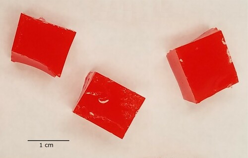
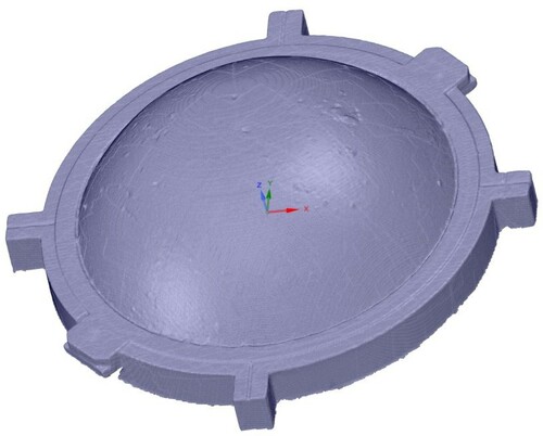
Tumours were all created simultaneously from a single batch of tumour material. The mixture was stirred constantly for 5 minutes and then 71.5 g of the mixture was immediately poured into an 85-mm-diameter polypropylene petri dish sprayed with mould release. The silicone/dish was immediately moved to the vacuum desiccator and degassed for 15 minutes. Then the vacuum was released and the silicone was allowed to cure in the dish. After curing, the silicone puck was removed from the dish and roughly cubical tumours⁸ were cut from the puck with a razor blade. Tumours were retained if they were between 1.95 and 2.05 g, and any outside that range were discarded. Figure 1 shows typical tumours.

Figure 1. Typical 1.95–2.05 g tumours before placement in a phantom.

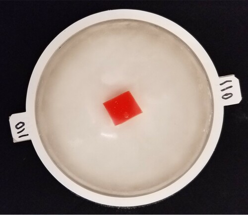
Tumour-containing phantoms were prepared in a similar manner to tumour-free phantoms, except that only 178 g of mixture was poured into the mould. Then, a tumour was suspended at an appropriate location in the liquid silicone using a paper clip. The silicone/ mould/tumour was immediately degassed for 15 minutes and then allowed to cure at least overnight. The paperclip was gently removed from the phantom and the phantom was demoulded. Next, only the flat surface of the phantom was coated with talcum powder and the phantom was placed on a tray and photographed, allowing us to identify the tumour radius with some precision. (Figure 2 shows the photograph of phantom Tumour B.)Due to the curvature of the phantom it was not possible to accurately photograph the height of the tumour within the tissue and we therefore made estimates based on manipulation of the phantom. Finally, the top surface of the phantom was coated with talcum powder. Note that once the talcum powder is applied to the surface it is possible to approximately, but not precisely, locate the tumour. Again, when not in use phantoms were stored in sealed polypropylene containers in a dark cabinet.

Figure 2. Top view of phantom Tumour B showing tumour location. (The restraining ring has a 110-mm inner diameter.)

3.2. Indentation device

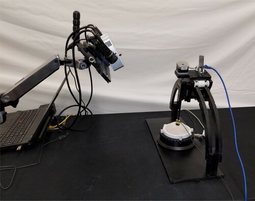
Figure 3 shows the device created to allow us to indent the surface of the phantom and then record the associated forces – we will refer to this device as the ‘Arc’.

Figure 3. Arc device used to indent the surface of the phantom and record associated forces. (Near the centre of the photo, a white phantom sits in a white tray on the black turntable. Black arches support the indenter mechanism, shown at the $\varphi =10$ degree angle. The rod connects the indenter mechanism through the yellow force sensor to the black indenter head.)

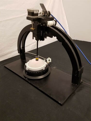
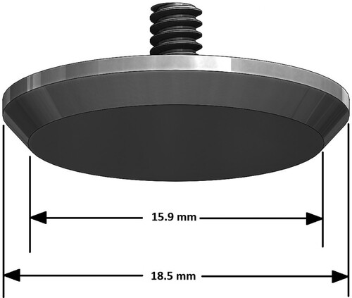
The phantom sits in a tray mounted on a turntable,⁹ and is surrounded by a 110-mm diameter restraining ring. (This restraining ring can be seen more clearly in Figure 2.) The turntable is fixed to the base of the Arc. Indentations are controlled by a stepper motor, lead screw, and linear slide mechanism mounted on the arches and the arches contain detents to fix the locations of that mechanism. The indentation rod is connected through a miniature s-beam load cell (100 g max load¹⁰) to the indenter head¹¹. Figure 4 schematically shows the indenter head geometry. The operation of the Arc is semi-automated – the indenter motion, turntable rotation, and force readings are computer-controlled but the movement of the indenter mechanism from one detent to the next on the arches is adjusted and locked in place manually.

Figure 4. Schematic of indenter head geometry.

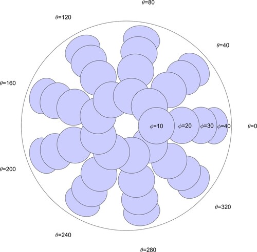
The geometry of the Arc controls the locations at which the indenter head contacts the phantom. The four detents on the arches cause the indenter rod to approach the phantom at angles (‘ϕ’) of 10, 20, 30, and 40 degrees from the vertical and approximately normal to the phantom surface. The turntable is rotated to azimuthal positions (‘θ’) of 0, 40, 80,…, 320 degrees. Figure 5 schematically shows a top view of the phantom with the indentation locations and the terminology for ϕ and θ.

Figure 5. Top view of phantom showing indenter locations. (ϕ is the angle the indenter makes with the vertical and θ is the azimuthal angle. This figure is drawn to scale.)

3.3. Phantom testing

For testing, phantoms are coated with talcum powder, placed in the testing tray, and fitted with a 110-mm restraining ring as indicated in the previous section. If the phantom has been used previously, the old powder is removed by gentle cleaning in lukewarm water and allowed to dry before it is again coated with talcum powder. The talcum powder on the phantom surface prevents sticking and makes the scan in the next step easier to capture.

Next, the sample is scanned with a structured light scanner¹² and the surface profile for the phantom and tray is exported as an STL file. Figure 6 shows the scanner/Arc orientation.After testing is complete, a phantom-specific finite element mesh is created by postprocessing the STL file. (This is described in detail in Appendix 1).

Figure 6. Orientation of scanner used to capture phantom geometry for finite element modelling (left, on arm near laptop) and Arc with phantom (right side) during testing.

Now the force readings at the 36 sites are recorded. The tray is aligned with $\theta =0$ and the indenter mechanism is adjusted to the $\varphi =10$ detent. At this site the process is:

• Move the indenter to a location a few mm above the phantom surface

• Zero the force sensor reading

• Advance the indenter into the phantom until the reading is between 11.5 and 12.5 g. Hold 1 second.

• Record the force (call this reading P1)

• Move the indenter out 3 mm and in again that same 3 mm. Hold 1 second.

• Record the force (reading P2)

• Advance the indenter an additional 3 mm into the phantom. Hold 2 seconds.

• Record the force (reading R1)

• Move the indenter out 6 mm and in again that same 6 mm. Hold 2 seconds.

• Record the force (reading R2)

The two readings P1 and P2 serve to precompress the sample and ensure that the indenter head is fully engaged with the phantom. The holds ensure that the force readings are stable. The final force value for this site (the force used as input to the numerical methods) is (1) $F_{exp}^i=\frac{R2+R1}{2}-\frac{P2+P1}{2}$(1) so that the experimental force $F_{exp}$ at site i is the difference between the average indented and precompressed values. Next the turntable is rotated 40 degrees to move to the next θ location, and another experimental force value is acquired. Turntable rotations continue until all θ values for this ϕ have been recorded, then the indenter mechanism is moved to the $\varphi =20$ detent, and so forth until all 36 force values have been acquired.

The inputs to the numerical methods described in the next section are the 36 force values and the STL of the phantom surface.

4. Numerical methods

Identifying the presence or absence of tumours within the healthy breast tissue based on surface force measurements is known as an ‘inverse parameter estimation’ problem and has been understood for many years to be computationally challenging [74].

The computational algorithms for the force-only stiffness mapping in this paper are similar to those we have used in our displacement-only work [8] in that they employ finite elements in combination with a genetic algorithm to solve the inverse problem. We made two key advances in our computational methodology to allow us to incorporate forces rather than displacements in our inverse solution approach: phantom-specific finite element meshes and a genetic algorithm cost function based on the correlation coefficient. This next section gives an overview of the computational algorithms for completeness and in order to provide context for the key advances.

4.1. Computational algorithms overview

We use a genetic algorithm to identify the tissue material property distribution that best fits our measured data:

• Randomly create an initial population of individuals with different material property distributions

• For each generation

  1. Evaluate each individual for its ‘fitness’

  2. Select top individuals as ‘parents’, discard others

  3. Mate parents to create new individuals (‘children’)

  4. Introduce mutations into some children

• (Continue until convergence)

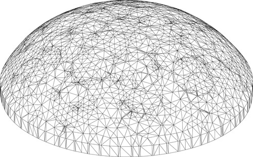
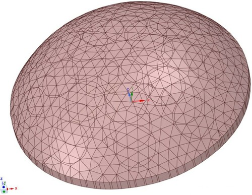
Finite element methods are used to evaluate individuals.¹³ We use a phantom-specific mesh derived from the phantom's STL scan– a mesh such as the one shown in Figure 7 would be typical (40 K nodes and 25 K elements). Appendix 1 gives details of the finite element methods and Section 4.2.1 explains the significance of this part of the process.

Figure 7. Typical phantom-specific finite element mesh generated from the geometry captured by the scanner. (40 K nodes and 25 K elements.)

The finite elements are nearly incompressible ($\nu =0.49$) 10-node tetrahedral displacement/pressure elements [75]. The mesh is the same for all of the individuals and the only differences between individuals are the material properties assigned to the elements– each element is assigned either ‘healthy’ (Young's Modulus 3.2 kPa) or ‘cancerous’ (22.6 kPa) tissue. The information about the individuals is coded into a ‘chromosome’ (see Figure 8) which lists the material properties for each of the elements.To reduce the size of the search space without coarsening the mesh, elements are grouped into 144 ‘clumps’ each of which is slightly larger than 1 cm${}^3$. All the elements in a given clump are assigned the same material property. Next, for each individual we (computationally) apply the indentations, record the reaction forces, and assess that individual's fitness.

Figure 8. Chromosome used to encode material property information for each individual ($E_h$ is healthy modulus, $E_c$ is cancerous modulus.) [8].

We use a ‘cost’ function to assess the individual's fitness. In general terms, the cost is a balance between the fit to the data and a regularizer which penalizes widely dispersed tumours. (2) $\text{Cost}=\text{(Error in Match to Measured Data)}+w\cdot \text{(Tumour Radius)}$(2) Because this is an ill-conditioned (inverse) problem, fitting the measured data exactly to the finite element individual's result produces answers that may be significantly affected by small measurement errors. The tumour radius is the mean relative size of the tumour in the finite element individual and serves as a regularizer which stabilizes the results. w is an adjustable weighting parameter which sets the balance between the fit to the data and the regularizer. Section 4.2.2 discusses the precise formulation of the cost and gives more details on the weighting parameter.

The lowest cost individuals are the most fit, and we choose 16 as parents for the next generation. Parents are mated in pairs to produce children. Once the children are created mutations are introduced in the children.

The most fit individual in the last generation is the stiffness map. In our cases we used 288 individuals and we terminated after 50 generations. Although terminating after a fixed number of generations would not be appropriate in clinical investigations, our algorithm routinely converges by this time. Additional details on the genetic algorithm may be found in [8].

4.2. Key advances

As mentioned earlier, we made two key advances in our computational methodology to allow us to incorporate forces rather than displacements in our inverse solution approach: phantom-specific finite element meshes (Section 4.2.1) and a genetic algorithm cost function based on the correlation coefficient (Section 4.2.2).

4.2.1. Phantom-specific finite element meshes

In moving from displacement-only to force-only stiffness mapping, we needed to implement higher-resolution phantom-specific finite element meshes in order to accurately model the indentation forces as described in Appendix 1.

For our displacement-only work [8], we used ellipsoidal approximations to the phantom geometry and imprinted the indenter patterns on that surface. We found a good surface displacement match between the finite element model and the experiments. Recall that we impose a particular displacement at the indenter. We were not able to capture experimental data immediately adjacent to the indenter due to camera angles. Hence, all of the data match happened starting a small distance away from the indenter and small meshing errors around the indenters caused little difficulty – the displacements away from the indenter depend primarily on the imposed displacement at the indenter and only weakly on the exact size of the indenter.

However, when we moved to a force-only method we found we needed substantially better resolution of the indentation site and overall phantom geometry to capture the force accurately. (As appropriate for a finite element method, we calculated the indentation forces as reaction forces on the restrained bottom of the phantom to eliminate issues with stress concentrations near the indentation site.) While the stress in the region near the indenter is not substantially affected by the exact indenter size the force is the stress times the area and hence errors in the indenter area are directly proportional to the error in the force. Since we wished to keep the controllable modelling errors well below the approximately 4 percent experimental errors we used care to create suitably accurate meshes around the indenters. Reviewing the regions around the indenters in Figure 7 shows how the details of the surface mesh around the overlapping indenter sites complicated the meshing. In addition, the placement of the phantom on the testing tray often results in variations from perfect symmetry that affect the forces. This results in small (on the order of 1 g) variations in forces as we rotate the turntable to move from one θ to another at the same ϕ (review Figure 5). These force variations can be captured with the phantom-specific finite element meshes but would not be captured by an ellipsoidal mesh.

We will need patient-specific meshes in clinical applications and our results suggest that the use of the scanner data to produce phantom-specific meshes was quite effective.

4.2.2. Cost function choice

The exact form of the Cost function is critical to the success of any genetic algorithm, and recall that we use (Equation 2(2) $\text{Cost}=\text{(Error in Match to Measured Data)}+w\cdot \text{(Tumour Radius)}$(2) ) a balance between the error in the match to the measured data and a tumour radius regularizer.

More precisely, we chose an error in the match to the measured data for a given finite element individual which is related to the correlation coefficient between its force predictions and the corresponding experimental readings. We chose this error measure because the correlation coefficient is independent of amplitude – since the force measurements depend directly on Young's modulus any inaccuracies in modulus would otherwise produce spuriously large errors in a more common error measure such as the root-mean-squared (rms) error.

The correlation coefficient for finite element individual j is (3) $C{C}_{F{E}_j}=\frac{{\displaystyle \sum _{i=1}^{N_{ind}}(F_{exp}^i-\overline{F_{exp}})(F_{F{E}_j}^i-\overline{F_{F{E}_j}})}}{\sqrt{{\displaystyle \sum _{i=1}^{N_{ind}}(F_{exp}^i-\overline{F_{exp}}{)}^2}}\sqrt{{\displaystyle \sum _{i=1}^{N_{ind}}(F_{F{E}_j}^i-\overline{F_{F{E}_j}}{)}^2}}}$(3) Here $F_{exp}^i$ is the experimentally measured force at indenter i, $F_{F{E}_j}^i$ is the predicted force at that same indenter for finite element individual j, $\overline{F_{exp}}$ is the mean of the experimentally measured forces, and $\overline{F_{F{E}_j}}$ is the mean of the predicted forces for finite element individual j. $N_{ind}$ is the number of indenters which is equal to the number of force readings, in our case 36. The first individual in the first generation is chosen to be tumour-free, and we will denote that correlation coefficient by $C{C}_{TF}$ and use it to normalize the error. The error for individual j is then taken to be (4) ${\text{(Error in Match to Measured Data)}}_j=\frac{1-C{C}_{F{E}_j}}{1-C{C}_{TF}}$(4) Since the range of the correlation coefficient is −1 to 1 and good fits are near 1, this error formula will always result in a positive number and good fits will have small errors.

The Tumour Radius for individual j is more precisely defined as (5) ${\text{(Tumour Radius)}}_j=\frac{R_{tumou{r}_j}}{R_{entire}}$(5) This tumour radius regularizer is the same as that used for our displacement-only stiffness mapping (see [8] for details). The values of the two components are volume-weighted mean radii for the tumour and the full domain – if we had a 0.5-cm radius spherical tumour inside a healthy tissue sphere of radius 5 cm then we would have ${\text{(Tumour Radius)}}_j=0.1$.

Hence, for any given individual the cost used to evaluate its fitness is (6) ${\text{Cost}}_j=\frac{1-C{C}_{F{E}_j}}{1-C{C}_{TF}}+w\cdot \frac{R_{tumo{r}_j}}{R_{entire}}$(6) Note that the Cost for the tumour-free finite element individual is always 1.

w is the regularizer weighting parameter and allows us to adjust the balance between the two terms in the cost function. If w is zero, then we fit the experimental data exactly but for inverse problems this often leads to poor performance since the solutions are extremely sensitive to small changes in the data (e.g. experimental errors). If w is too large, then the prediction produced by the algorithm is always tumour-free because that will be the lowest cost. In this work, we would like to find a single w that correctly classifies all of the experiments as tumour-free or tumour-containing phantoms. (As more experience and data are acquired, it may be possible to adaptively choose w based on the data, but we do not have that experience/data at this point.)

For each test, there is a particular value of w at which the test will cross from being correctly classified to being incorrectly classified, and we denote that value as $w_{cross}$.

5. Results and discussion

We created four tumour-free phantoms and four tumour-containing phantoms, and ran four tests on each phantom for a total of 32 tests. Figure 9 schematically shows the approximate vertical locations of the tumours in the four tumour-containing phantoms. Figure 10 shows the approximate radial locations of the tumours for the 16 tests and also indicates the indenter centres.Notice that Tumour B is located deep in the centre of the tissue. (We will refer to this as a ‘deep centre tumour’.) That phantom was randomly placed for each of its four tests, while the other three tumour-containing phantoms were oriented (approximately) at four different angles for testing. Tumour-free phantoms were randomly placed.

Figure 9. Schematic of phantom side view showing approximate vertical locations of the tumours in the four tumour-containing phantoms.

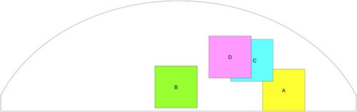
Figure 10. Schematic of phantom top view showing approximate radial locations of the tumours in the tests of the four tumour-containing phantoms. (‘*’ denotes the location of the indenter centres).

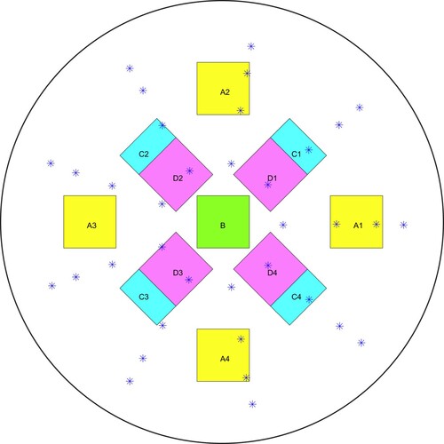
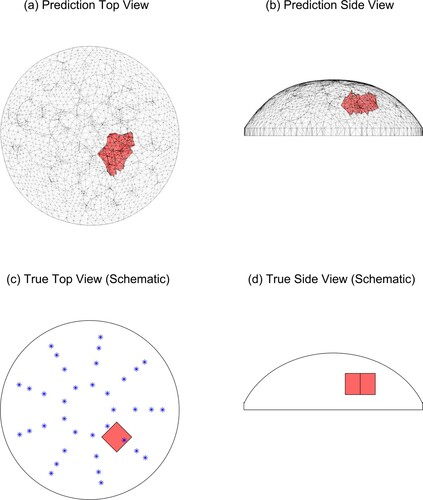
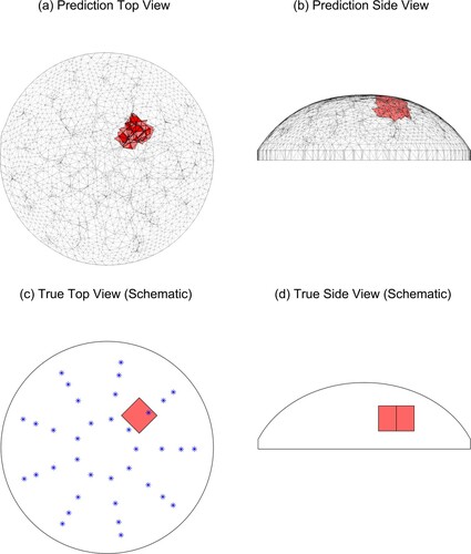
Figure 11 shows the predicted tumour location with w = 2.0 for Tumour C, test 4 (‘TC4’) and also schematically shows the location of the tumour in the experimental phantom and the locations of the indenter centres. The agreement between the true and predicted tumour location is excellent.Figure 12 shows a more typical prediction with w = 2.0 for the same physical phantom, this time tested at 45 degrees (TC1) and also schematically shows the location of the tumour in the experimental phantom. In this case, the predicted tumour is in the correct radial and azimuthal location but the tumour is too close to the surface. Since we are investigating this method as a preliminary screening tool only, the accurate radial/azimuthal location is more important than the tumour elevation and this is a good result.

Figure 11. Predicted and true results for Tumour C, test 4. (‘*’ denotes the location of the indenter centres. Note that the vertical line in the middle of the tumour in (d) is the corner of the cube.)

The tumour size in the prediction is constrained by the finite element clumps and so it is not expected to be very accurate. Recall (Section 4.1) that we divide the finite element mesh into 144 centrally located clumps of elements, with an average volume of 1 cc, and each clump is assigned the same material property. These clumps are created with a systematic radial and vertical pattern based solely on the finite element mesh geometry [8] and do not change during the analysis. For example, Figure 11 shows two adjacent clumps as the predicted tumour. The roughly cubical physical tumours placed in the phantom had a volume of approximately 1 cc, but there is little chance that the physical tumour actually has the same centre as a single clump. The algorithm may choose more than one clump as the best fit in order to span the true tumour location and improve the fit to the measured data, but this means that the tumour size prediction is not expected to be very accurate.

Figure 12. Predicted and true results for Tumour C, test 1. (‘*’ denotes the location of the indenter centres. Note that the vertical line in the middle of the tumour in (d) is the corner of the cube.)

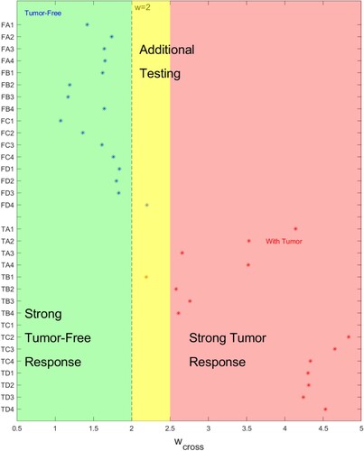
The results depend on the value chosen for the regularizer w, and the results shown are at w = 2.0. With this choice for the regularizer, 15/16 tumour-free cases are correctly identified as tumour-free, and 16/16 tumour-containing cases are correctly identified. One tumour-free test resulted in a false positive.

Figure 13 summarizes the results for all 32 tests and indicates the effect of the regularizing parameter.

Figure 13. Correct identification of tests at w = 2.0 occurs for 15/16 tumour-free samples and 16/16 tumour-containing samples. (Blue lines indicate range of w for correct identification of tumour-free samples. Red lines indicate range of w for correct identification of tumour-containing samples. Horizontal axis indicates w value, vertical axis gives test name.)

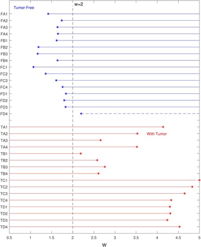
Tumour-free tests are shown in the top half of the plot (‘FA1’ is tumour-free sample A, test 1). For each tumour-free test, there is a minimum value of w required to properly regularize the inverse prediction, and above that minimum value the results will continue to be classified as tumour-free. The range over which a given tumour-free test is classified correctly is shown with blue lines – the ‘*’ is located at $w_{cross}$ and proceeds to the right. Test FD4 (the single false positive test) needed a w larger than 2.0 for correct classification and is shown with a dashed line. Tumour-containing tests are shown in the bottom half of the plot (‘TA1’ is tumour-containing sample A, test1). For a tumour-containing test, there is a maximum value of w that is allowed before the inverse prediction is over-regularized and the tumour prediction is suppressed. The range over which a given tumour-containing test is classified correctly begins at zero and ends at $w_{cross}$, shown with red lines that end at the red ‘*’.

TB1 and FD4 cannot both be classified correctly because their ranges of correct classification do not overlap. TB1 requires a w less than 2.19 for correct classification and FD4 requires a w greater than 2.20 for correct classification. Recall that Tumour B is in the deep centre of the phantom so that it seems logical that it would be difficult to distinguish from a tumour-free sample, however, three other tests of the same phantom were not as problematic. To check our results, the experimental data for TB1 and FD4 were reprocessed three times and the figure shows the worst result for each experiment. The overlap appears to be a real phenomena in the experimental data rather than a flaw in the processing. Based on this overlap we chose a classification w = 2.0 to produce a false positive for FD4 rather than a false negative for TB1.

Recall that $w_{cross}$ is the value of w at which a test will cross from being correctly classified to being incorrectly classified. Figure 14 presents the results for $w_{cross}$ in a different light. When $w_{cross}$ is far from the chosen regularizing parameter w = 2.0 there is little chance of misclassifying the sample and we have characterized those regions as strong responses. There is a region close to w = 2.0 where additional testing should occur.

Figure 14. $w_{cross}$ for a given test indicates the strength of the classification. (Horizontal axis indicates $w_{cross}$ value, vertical axis gives test name.)

The success of a genetic algorithm in classifying tests depends heavily on the cost function chosen and we used a cost measure which includes an error measure based on the correlation coefficient (review Equation 4(4) ${\text{(Error in Match to Measured Data)}}_j=\frac{1-C{C}_{F{E}_j}}{1-C{C}_{TF}}$(4) ) which appears to be a powerful means of discriminating between the test sets. (Recall that we chose this error measure because the correlation coefficient is independent of amplitude.) In the cost equation (Equation 4(4) ${\text{(Error in Match to Measured Data)}}_j=\frac{1-C{C}_{F{E}_j}}{1-C{C}_{TF}}$(4) ) we normalize the error by $1-C{C}_{TF}$ where $C{C}_{TF}$ is the correlation coefficient between a tumour-free finite element model and the experimental data. 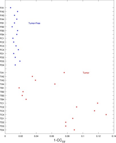Figure 15 plots $1-C{C}_{TF}$ for each of the tests.It is clear from the plot that the error for the tumour-free model will be very small for tumour-free phantoms and high for the tumour-containing phantoms. The weakest separation occurs (again) for the deep centre tumours in TB1 through TB4.

Figure 15. Errors for tumour-free model are small for tumour-free phantoms and high for tumour-containing phantoms. (Horizontal axis gives the error ($1-C{C}_{TF}$), vertical axis gives test name.)

The difficulty in identifying a deep centre tumour is a physical constraint of any surface-force-based approach – there is very little change in the measured forces at the surface due to the tumour. Figure 16 shows the force measurements for a tumour-free test. Note that although the tumour-free sample is nominally symmetric there are small variations in readings due to experimental noise and geometry variations from phantom placement. Figure 17(a) shows the fit between the experimentally measured data and the tumour-free finite element model results for that same test. Figure 17(b) shows the experimental data and the tumour-free finite element model results for an easily identified tumour (TC1). There is a strong signal in the vicinity of the tumour and the fit to the tumour-free model is clearly poor which is good since the phantom contains a tumour. Figure 17(c) provides the same data for the deep centre tumour which was most difficult to identify (TB1). There is very little difference between the graphs in (a) and (c) which explains why it is difficult to identify (c) as tumour-containing. The most notable difference between the two data sets occurs at high elevations – at $\varphi =10$ degrees the readings for the tumour-containing test are almost the same as at $\varphi =20$ degrees, while for the tumour-free test the values are lower at $\varphi =10$. However, this difference is on the order of 1 gram out of a 30 gram reading. For some deep centre tumours the fit between the experimental data and the model results was such that it was just possible to identify the tumour, but for (TB1) it was not possible. As inverse solutions are sensitive to noise it is reasonable to infer that the experimental noise in the TB1 case was sufficiently high that it caused the algorithm to predict incorrectly.

Figure 16. Measured forces for a tumour-free phantom test (FC1) (There are 9 azimuthal test sites at $\theta =0,40,\dots 320$ degrees for each of the elevation angles ϕ.)

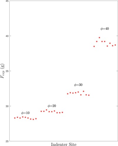
Figure 17. Measured forces (red *- symbols) and tumour-free finite element model results (blue o symbols) for three tests: (a) a tumour-free test (FC1), (b) a test with an easily identified tumour (TC1), and (c) the most difficult-to-identify deep centre tumour (TB1). (Forces are normalized to zero mean. There are 9 azimuthal test sites at $\theta =0,40,\dots 320$ degrees for each of the elevation angles ϕ.)

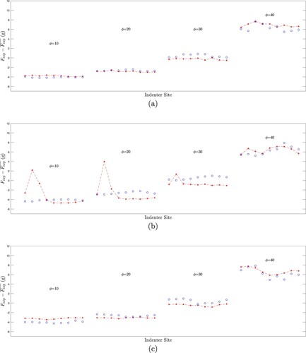
Since deep centre tumours produce only small variations in the forces we can measure at the surface we feel our algorithm has performed well in classifying these cases.

Our approach correctly classified 31/32 tests, with one false positive tumour-free case, for 2g tumours (approximately 1.3 cm cubes). To put this in context, the American Joint Committee on Cancer [76] grades cancers in part by their tumour size. Breast cancer tumours less than 2 cm where the cancer has not spread to other sites are collected into the lowest risk group for invasive cancers with a relative 5 year survival rate of 100% [77]. Hence, the ability to detect such tumours reliably would be important to patient survival.

In our previous work [8], we used a similar indentation approach but measured surface displacement data on the full phantom surface instead of measuring applied surface forces. Each measurement modality has advantages and disadvantages. The displacement measurements were more difficult to acquire than the force values, but there was a clear separation between the $w_{cross}$ values for the tumour-free samples and the tumour-containing samples (no samples fell between 0.109 and 0.305). Hence we were able to correctly classify 12 tumour-free and 14 tumour-containing samples. Note that, for a tumour-free sample the surface displacements will be independent of the tissue modulus. This is due to the fact that all of our boundary conditions are either a specified displacement (at the indenter and the base of the phantom) or a traction-free condition on the tissue surface. Hence, the actual modulus drops out of the solution. For a tumour-containing phantom the surface displacements depend solely on the ratio of the tumour modulus and the background modulus. In later examination [78], we also found that the surface displacement data over a large fraction of the surface contributed to the ability to classify the samples correctly – there are many samples on the surface for a single indentation site (unlike the force data that produces a single value) so that experimental errors at one point on the surface are less damaging. However, the amplitude of the displacement signal is always less than the indentation depth so that even tumours relatively close to the surface do not produce a larger signal. The force reading provides a very strong signal for those same tumours (hence it is used in manual palpation) but forces alone struggle with classification of deep tumours. Sensing the force allows us to easily identify when the indenter has made full contact with the surface so that the results can reasonably be modelled as in the linear regime and the additional effort to take a measurement of the indentation force is trivial. The force data also allows us to estimate the healthy tissue stiffness which may be useful in tuning our finite element models and adapting the regularization parameter.

Our experience with force measurements and displacement measurements should allow us, in future work, to combine forces and displacements in the cost function. Consider a combined cost function which is a generalization of Equation (2(2) $\text{Cost}=\text{(Error in Match to Measured Data)}+w\cdot \text{(Tumour Radius)}$(2) ): $\begin{array}{rl}Cost& =\alpha \ast \text{(Error in Match to Displacement Data)}\\ & +(1-\alpha )\ast \text{(Error in Match to Force Data)}\\ & +w\ast \text{(TumourRadius)}\end{array}$(Recall that each term has been nondimensionalized.) When $\alpha =1$ we recover the displacement method, and when $\alpha =0$ we recover the force method. For a combined method we will adjust α to balance the relative significance of the displacement and force data and w to penalize tumour radius. Because the parameter space will be two-dimensional identifying appropriate values for α and w based on experimental data may take some effort but should be feasible. Our experience with each sensor modality separately should help inform this future research.

As discussed in the introduction, we ultimately seek to automate and refine the manual breast exam process using measured data on the breast surface in combination with formal inverse techniques to produce 3D maps of the stiffness inside the breast tissue. The experimentally validated computational advances we have discussed here are a crucial step towards that goal, but have a number of limitations. Clinically, these maps will only identify stiff regions within the tissue and some benign tissues are stiff while some cancerous tissues may not be stiff enough to detect. This is a fundamental limitation of the method but still may permit more cancers to be detected earlier. In addition, these experiments were performed in tightly controlled conditions which will not be present in clinical settings. We have presented results from a typical-sized breast phantom. Our results suggest that smaller phantoms should perform better, and nothing in the computational algorithms limits the domain size. However, larger phantoms and phantoms with background stiffness inhomogeneities will need to be examined in the future. The effects of varying tumour stiffnesses relative to the background tissue will also need to be examined. Nothing in the computational algorithms limits the number of different stiffnesses we can include although the search space will increase and more regularization may be required. However, it is clear that if our methods are unsuccessful in the current tightly controlled conditions they are certainly unsuitable. Knowledge gained from this successful research should allow us to create more robust and adaptable techniques for the next phase of the project.

We believe that combining surface displacement and force measurements will yield a method that is more robust than either method alone, and that will be the focus of our future work.

6. Summary and future work

Our long-term goal is to automate and refine the manual breast exam process using measured data on the breast surface in combination with formal inverse techniques to produce 3D maps of the stiffness inside the breast tissue. In previous work, we successfully validated the use of surface displacement-only data with a genetic algorithm/finite element method for stiffness mapping. Here we have introduced new experimental methodologies for force measurements on silicone phantoms and key algorithmic improvements (phantom-specific finite element meshes and cost functions based on the correlation coefficient) to allow us to validate the use of force-only data for stiffness mapping.

We ran 16 tests on 180 g silicone tumour-free phantoms and 16 tests on phantoms containing 2 g tumours. One tumour-free test resulted in a false positive and the remaining 31/32 tests were correctly classified. Predicted and actual tumour locations agreed well for correctly-classified samples. These results are promising but clearly a great deal of work remains to be done before stiffness mapping could be applied as a screening tool in clinical settings.

In the near future, we will extend the method to combine force and displacement measurements in the experiment and the computational algorithm. By examining each measurement modality separately we have gained valuable insight into appropriate cost functions and each modality's strengths and weaknesses. A one-norm cost function worked best for our displacement-only studies, while a cost function based on the correlation coefficient worked well in this force-only study due to its amplitude-independence. Because we are using a genetic algorithm, the cost function for the combined displacement and force method can easily incorporate those distinct error measures along with our regularizer based on the tumour radius. Displacement-only measurements are less sensitive to accurate meshing than force-only measurements but that implies that the phantom-specific meshes and force data yields additional information. Displacement-only measurements naturally incorporate redundancy but force-only measurements show stronger signals for tumours that are closer to the tissue surface.

We anticipate that the combination of force and displacement measurements will be more effective for our stiffness mapping approach than either measurement modality separately.

Acknowledgements

This work was supported by generous contributions to the Lawrence J. Giacoletto endowment. This work used the Extreme Science and Engineering Discovery Environment (XSEDE), which is supported by National Science Foundation grant number ACI-1548562. Resources were obtained through the Texas Advanced Computing Center at the University of Texas at Austin.

Disclosure statement

No potential conflict of interest was reported by the author(s).

Additional information

Funding

This work was supported by Lawrence J. Giacoletto Endowment [Rose-Hulman Institute of Technology].

Notes

1 A-341 from Factor II, Inc.

2 Dow Xiameter PMX200 50 cs silicone fluid, Ellsworth Adhesives

3 FI-204 Functional Intrinsic II Silicone Coloring System, Factor II, Inc.

4 IMUSA 10-oz Multicolor Salsa Dish

5 Mann Release Technologies Ease Release 200

6 Bel-Art ‘Space Saver’ Polycarbonate Vacuum Desiccator F42025-000

7 Johnson's Baby Powder, Original

8 For our purposes, St. Venant's principle [73] means that the exact shape of the tumour does not affect the surface forces measured at a distance from the tumour. Thus, any similarly sized tumour of the same stiffness would produce the same result. We address this in more detail in Appendix A.4.

9 HP 3D Automatic Turntable Pro

10 Futek LSB200. This cell has a rated output (RO) of 100 g, a nonlinearity and hysteresis of $\pm 0.1$% of RO, and a nonrepeatability of $\pm 0.05$% of RO. The load cell output is recorded to the nearest 0.1 g after signal conditioning.

11 McMaster-Carr 5/8”x 3/32” Contact Points for Dial Indicator, #20625A421

12 HP 3D Scanner Pro S3 with dual cameras

13 This finite element code is a custom, fully validated code which is integrated with the genetic algorithm for efficiency.

Appendices

Appendix 1. Finite element modelling details

An experiment-specific geometry for our finite element mesh is created by postprocessing the file generated by scanning the phantom in the test setup before the indentation testing. Thus the mesh for each experiment is customized to the particular geometry.

A.1. Geometry

The scan produces a high-resolution (570 K triangles) STL file of the top surface geometry of the phantom and sampling tray, as shown for a typical phantom in Figure A1. We reorient the scan to a coordinate system defined by the axes shown schematically in Figure A1.The resulting STL file is loaded into the ANSYS Workbench SpaceClaim modelling package. Within SpaceClaim we clip and smooth/reduce the STL file to surface triangles with a 5-mm size specification. This is converted to a solid object and the base is extruded slightly to represent the unscanable portion of the phantom below the surface of the tray. Next, a sequence of 36 9.25 mm cylinders are used to imprint the surface at the locations where the indenter touches the surface. The resulting solid geometry for a typical phantom is shown in Figure A2 and it is possible to see a number of the (circular) indentation locations in that view.

Figure A1. Typical STL geometry produced by scanning the phantom and tray.

A.2. Finite element model and programming details

The solid object geometry is loaded into ANSYS Workbench Mechanical for mesh generation. The 5 mm top surface triangles serve as a constraint on the surface mesh, and a 5-mm maximum element size constraint and a 0.1-mm defeaturing tolerance is applied to the body. Note that this element size is a constraint on the maximum characteristic element length and the average element size is much lower (typically 2.2 mm). The mesh consists of straight-sided quadratic tetrahedral elements and a typical mesh with 40 K nodes and 25 K elements is shown in Figure 7.

Figure A2. Typical solid geometry for the phantom.

This mesh is exported and converted to a input file for our custom finite element code. The finite elements themselves are nearly incompressible ($\nu =0.49$) displacement/pressure elements [75]. The finite element solver is a custom, fully validated code which is integrated with the genetic algorithm. For the forward solution 3 mm indentations are applied by prescribing nodal displacements on an indentation patch, with the nodal displacements along the indenter rod axis. Thus we model the indenter as though it were ‘stuck’ to the surface and touching the surface uniformly from the outset. The flat base of the phantom and the rim of the phantom below the tray surface are modelled as completely fixed (‘stuck’ to the sample plate). The indentation forces are calculated from the reaction forces on the flat base and rim of the phantom.

The forward matrix equations are solved with the Intel PARDISO Direct Solver with low rank updates to adjust the matrix for the 36 different indenter load cases. MPI is used to implement the parallelization for the inverse solution. We used Stampede 2 at University of Texas Austin through the NSF XSEDE supercomputing allocation program. A typical complete inverse solution used 288 tasks on 6 nodes (48 tasks/node) and took less than four hours of wall-clock time.

A.3. Mesh convergence

We wish to ensure a balance between required computing time and the desire that the mesh represent an accurate solution given the modelling assumptions. Hence, we examined the convergence of the forward-predicted forces for various meshes. Figure A3 shows the rms error between the forces for a particular mesh and the forces for a mesh created from the same geometry with a 2-mm maximum element size (average element size 1.3 mm).All of the errors are less than 1.5%.

Figure A3. RMS force errors are small for all meshes considered.

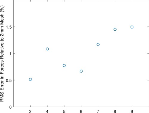
Table A1 shows the mesh statistics. For meshes with a maximum element size larger than 5 mm, the mesh is constrained by the surface triangulation to have a large number of surface elements and only the interior elements become larger. Therefore we see only moderate reductions in mesh degrees-of-freedom for the larger-element mesh specifications. When the maximum element size drops below 5 mm the surface mesh, too, must be refined and significantly more elements are required. Hence, we selected the 5 mm mesh for our modelling.

Table B1. Mesh statistics for convergence study (‘Characteristic Elem’ is the characteristic element length reported by ANSYS).

Max Elem	Characteristic Elem (mm)							Serial
Size (mm)	Min	Max	Ave	Std Dev	Nodes	Elements	DOF	Run Time (s)
9	0.04	8.9	2.0	1.5	25456	15009	71400	90
8	0.03	8.1	2.1	1.5	26319	15637	73737	97
7	0.03	7.0	2.1	1.5	27874	16751	77958	129
6	0.04	5.8	2.2	1.1	30861	18888	86367	170
5	0.04	5.2	2.2	1.1	39514	24638	111129	264
4	0.04	3.9	2.1	0.8	59580	38279	166713	648
3	0.04	3.0	1.8	0.5	104499	70566	295611	2293
2	0.04	2.0	1.3	0.2	298799	210492	859644	20241

A.4. Verification of St. Venant's principle

In the main body of the paper, we justified the use of roughly cubical tumours by invoking St. Venant's principle. It is also possible to use forward simulations to verify that the shape of the tumour does not substantially influence the force profiles on the phantom surface. We simulated a tumour with volume of 2 cm${}^3$ centred at roughly the location of Tumour C placed at 45 degrees (the case from Figures 12 and 17 b). We simulated three different tumour shapes: a clump of elements chosen from the tumour-free mesh, a sphere of elements, and a cube of elements. The rms error for the surface forces from the three tumour shapes showed variations comparable to the mesh errors in Figure A3: errors for the cube relative to the clump were 1.1% while errors for the sphere relative to the clump were 0.9%. Thus as St. Venant's principle indicates, the shape of the tumour does not have significant effects on the surface forces.

Appendix 2. Silicone material modulus characterization

Cylindrical moulds (35 mm diameter) for modulus testing were coated with mould release. All silicone mixtures were created by weight in polypropylene containers. After creation, the mixture was stirred for 5 minutes then 20 grams of mixture was poured into each of three moulds. The moulds were degassed in a vacuum desiccator for 15 minutes to remove bubbles, then the vacuum was released and the moulds were allowed to sit overnight. (The nominal cure time for the soft gel silicone is 1 hour, although we found that the addition of the silicone fluid increased the cure time to a few hours.)

The following day the three test samples were removed from the moulds. The resulting samples were h = 21 mm tall and D = 35 mm in diameter and had a smooth side (from the bottom of the mould) and a rougher top side due to the meniscus of the fluid. We used a Shimadzu EZ-SX 200N texture analyser to perform compression testing on the samples. Each sample was tested five times with the smooth side up and five times with the rougher side up. The testing protocol was a follows:

• Sample was visually centred on the testing platform.

• Compression plates were brought together until the force reading was 0.03 N.

• Compression plates were closed 2 mm at 2.5 mm/s.

• Compression plates were held at that deflection for 20 s.

• Compression plates were opened 12 mm at 0.5 mm/s.

• Sample was lifted and reset on the testing platform for the next test.

Data was exported for analysis in MATLAB.

Samples demonstrated widely varying force–deflection curve slopes for the compression loading but very consistent force-deflection curves for the unloading. We found that the sample often stuck to the compression plates and we believe that the varying compression force–deflection curves were due to the low preload, sample surface irregularities, and air entrapment at the compression plates. Hence, we used the unloading curves to estimate the sample stiffness.

We used a lower-strain portion of the unloading curve to estimate an apparent Young's modulus ($E_{apparent}$) for each sample test. The portion of the curve was defined to start at 0.05 of the maximum force for that sample and extended to a strain of 0.02 relative to that starting location. We used a linear fit to that region for each test individually which generated 10 values for $E_{apparent}$ for each sample. Figure A4 shows the stress–strain data for the 10 tests of a single sample.

Figure A4. A typical set of stress–strain data for the 10 tests of a single sample. Notice that a linear elastic material model appears reasonable for this strain range and that the slope of the data ($E_{apparent}$) is similar for all 10 tests.

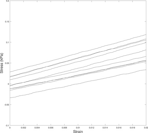
Notice that a linear elastic material model appears reasonable for this strain range and that the slope of the data ($E_{apparent}$) is similar for all 10 tests.

Because the boundary conditions for our testing were closely approximated by stick conditions we corrected $E_{apparent}$ to $E_{true}$ using a correlation equation derived from a finite element model of the test. We created a linear finite element model of the sample geometry (h = 21 mm tall and D = 35 mm in diameter) and applied sticking boundary conditions to the bottom plate and prescribed displacements to the top plate (0 in the tangential direction and δ in the normal direction). By using a nearly incompressible material model with Poisson's ratio $\nu =0.49$ and a particular $E_{true}$ we could calculate the $E_{apparent}$ from the model reaction force $F_{reaction}$: (A1) $E_{apparent}=F_{reaction}\frac{4h}{\pi \delta D^2}$(A1) Note that the boundary condition restraint causes $E_{apparent}$ to be larger than $E_{true}$.

Finally, we computed the mean and standard deviation of the 30 values of $E_{true}$ to arrive at our best estimate of the mixture modulus.

B.1. Functional testing

The linear elastic material model appeared valid up to a strain of at least 0.02. We did additional testing to confirm that the phantoms were behaving in a linear elastic fashion by checking the force–deflection curves for indentations on tumour-free phantom ‘A’. We placed the phantom in the arc system, but instead of the standard indentation testing we indented 0.4 mm at a time, recording the force. Figure A5 shows the resulting force–deflection curves for the $\varphi =10$ location. Recall (Section 3.3) that we use a precompression of 11.5−12.5 g for the actual indentation testing, so the figure shows the force–deflection curves relative to the precompression average of 12 g. The linear fit to the force–deflection data confirms that the silicone phantoms should behave in a linear fashion well past the standard indentation of 3 mm.

Figure A5. Force–deflection curves for indentation of a tumour-free phantom showing linear behaviour for significant indentation depths. The force is measured relative to a 12 g precompression, and the indentation depth is relative to the depth at 12 g of force. (‘*’ measured data; ‘–’ linear fit to measured data.)

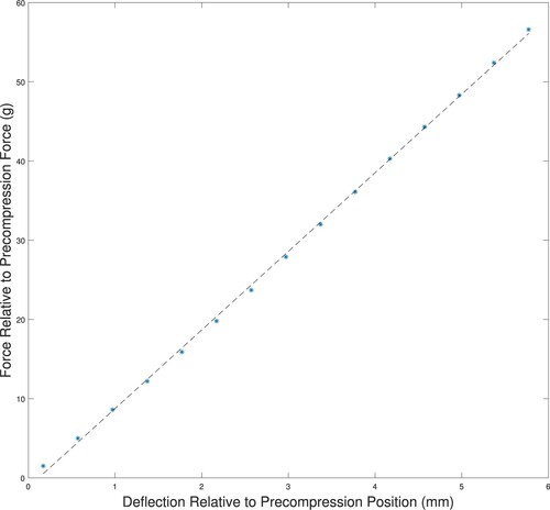
In our testing, we used a 1-second stabilization time for the precompression readings and a 2-second stabilization time for the full 3 mm indentation and observed little change in the force readings after those hold times. (Readings changed by less than 0.1 gram over many seconds.)

References

- Radiology Society of North America. http://www.radiologyinfo.org/, 2020.
- National Cancer Institute, Division of Cancer Epidemiology and Genetics. https://dceg.cancer.gov/news-events/news/2017/breast-density, 2020.
- Samani A, Zubovits J, Plewes D. Elastic moduli of normal and pathological human breast tissues: an inversion-technique-based investigation of 169 samples. Phys Med Biol. 2007;52:1565–1576.
- Greenleaf JF, Fatemi M, Insana M. Selected methods for imaging elastic properties of biological tissues. Annu Rev Biomed Eng. 2003;5:57–78.
- Olson L, Throne R. An inverse problem approach to stiffness mapping for early detection of breast cancer. Inverse Probl Symposium. 2012.
- Olson LG, Throne RD. An inverse problem approach to stiffness mapping for early detection of breast cancer. Inverse Probl Sci Eng. 2013;21(2):314–338.
- Olson L, Throne R. Early detection of breast cancer through an inverse problem approach to stiffness mapping: 3D results and variations in properties. Proceedings of the 12th U.S. National Congress on Computational Mechanics, 2013.
- Olson LG, Throne RD, Nolte AJ, et al. An inverse problem approach to stiffness mapping for early detection of breast cancer: tissue phantom experiments. Inverse Probl Sci Eng. 2019;27(7):1006–1037.
- Doyley MM. Model-based elastography: a survey of approaches to the inverse elasticity problem. Phys Med Biol. 2012;57:R35–R73.
- Parker KJ, Doyley MM, Rubens DJ. Imaging the elastic properties of tissue: the 20 year perspective. Phys Med Biol. 2011;56:1–29.
- Alam SK, Garra BS. Tissue elasticity imaging. Amsterdam: Elsevier; 2020.
- Li G-Y, Cao Y. Mechanics of ultrasound elasticity. Proc R Soc. A. 2017;473:20160841.
- Bamber J, Cosgrove D, Dietrich CF, et al. EFSUMB guidelines and recommendations on the clinical use of ultrasound elastography. Part 1: basic principles and technology. Ultraschall Med. 2013;34:169–184.
- Săftoiu A, Gilja OH, Sidhu PS, et al. The EFSUMB guidelines and recommendations for the clinical practice of elastography in non-hepatic applications: update 2018. Ultraschall Med. 2019;40:425–453.
- Shiina T, Nightingale KR, Palmeri ML, et al. WFUMB guidelines and recommendations for clinical use of ultrasound elastography: Part 1: basic principles and terminology. Ultrasound Med Biol. 2015;41(5):1126–1147.
- Barr RG, Nakashima K, Amy D, et al. WFUMB guidelines and recommendations for clinical use of ultrasound elastography: Part 2: breast. Ultrasound Med Biol. 2015;41(5):1148–1160.
- Bayat M, Nabavizadeh A, Kumar V, et al. Automated in vivo sub-hertz analysis of viscoelasticity (SAVE) for evaluation of breast lesions. IEEE Trans Biomed Eng. 2018;65(10):2237–2247.
- Bernal M, Chamming's F, Couade M, et al. In vivo quantification of the nonlinear shear modulus in breast lesions: feasibility study. IEEE Trans Ultrason Ferroelectr Freq Control. 2016;63(1):101–109.
- Goswami S, Ahmed R, Doyley MM, et al. Nonlinear shear modulus estimation with bi-axial motion registered local strain. IEEE Trans Ultrason Ferroelectr Freq Control. 2019;66(8):1292–1303.
- Hoerig C, Ghaboussi J, Insana MF. Data-driven elasticity imaging using cartesian neural network constitutive models and the autoprogressive method. IEEE Trans Med Imaging. 2019;38(5):1150–1160.
- Seidl DT, Oberai AA, Barbone PE. The coupled adjoint-state equation in forward and inverse linear elasticity: incompressible plane stress. Comput Methods Appl Mech Eng. 2019;357:112588.
- Patel D, Tibrewala R, Vega A, et al. Circumventing the solution of inverse problems in mechanics through deep learning: application to elasticity imaging. Comput Methods Appl Mech Eng. 2019;353:448–466.
- Wellman PS. Tactile imaging [dissertation]. Harvard University; 1999.
- Wellman PS, Dalton EP, Krag D, et al. Tactile imaging of breast masses. Arch Surg. 2001;136:204–208.
- Kaufman CS, Jacobsen L, Bachman BA, et al. Digital documentation of the physical examination: moving the clinical breast exam to the electronic medical record. Am J Surgery. 2006;192(4):444–449.
- Weiss RE, Hartanto V, Perrotti M, et al. In vitro trial of the pilot prototype of the prostate mechanical imaging system. Urology. 2001;58(6):1059–1063.
- Niemczyk P, Cummings KB, Sarvazyan AP, et al. Correlation of mechanical imaging and histopathology of radical prostatectomy specimens: a pilot study for detecting breast cancer. J Urol. 1998;160:797–801.
- Sallaway L, Magee S, Shi J, et al. Detecting solid masses in phantom breast using mechanical indentation. Exp Mech. 2014;54:935–942.
- Kearney TJ, Airpetian A, Sarvazyan A. Tactile breast imaging to increase the sensitivity of breast examination. J Clin Oncol. 2004;22(14S):1037.
- Helvie MA, Carson PL, Saravazyan A, et al. Mechanical imaging of the breast: a pilot trial. Ultrasound Med Biol. 2003;29(5S):S112.
- Egorov V, Tsyuryupa S, Kanilo S, et al. Soft tissue elastometer. Med Eng Phys. 2008;30:206–212.
- Egorov V, Sarvazyan AP. Mechanical imaging of the breast. IEEE Trans Med Imaging. 2008;27(9):1275–1287.
- Egorov V, Kearney T, Pollak SB, et al. Differentiation of benign and malignant breast lesions by mechanical imaging. Breast Cancer Res Treatment. 2009;118(1):67–80.
- Egorov V, van Raalte H, Sarvazyan AP. Vaginal tactile imaging. IEEE Trans Biomed Eng. 2010;57(7):1736–1744.
- Sarvazyan A, Egorov V. Mechanical imaging – a technology for 3-d visualization and characterization of soft tissue abnormalities. A review. Curr Med Imaging Rev. 2012;8(1):64–73.
- van Raalte H, Egorov V. Characterizing female pelvic floor conditions by tactile imaging. Int Urogynecological J. 2015;26:607–609.
- Kaufman CS, Son JS, Yered E, et al. Clinical studies of palpation imaging of the breast on over 1000 patients. 2014 San Antonio Breast Cancer Symposium, vol. P1-02-09, 2014.
- Peterson J. Introduction to suretouch for clinicians. https://sureinc.us/physician-introduction-1/, 2017.
- Xu X, Gifford-Hollingsworth C, Sensenig R, et al. Breast tumor detection using piezoelectric fingers: first clinical report. J Am Coll Surg. 2013;216(6):1168–1173.
- Xu X, Chung Y, Brooks AD, et al. Development of arry piezoelectric fingers towards in-vivo breast tumor detection. Rev Sci Instrum. 2016;87:124301.
- Yegingil H, Shih WY, Shih W-H. Probing model tumor interfacial properties using piezoelectric cantilevers. Rev Sci Instrum. 2010;81(095104):1–9.
- Yegingil H, Shih WY, Shih W-H. All-electrical indentation shear modulus and elastic modulus measurement using a piezoelectric cantilever with a tip. J Appl Phys. 2007;101(054510):1–10.
- Yegingil H, Shih WY, Shih W-H. Probing elastic tissue modulus and depth of bottom-supported inclusions in model tissues using piezoelectric cantilevers. Rev Sci Instrum. 2007;78(115101):1–6.
- Szewczyk ST, Shih WY, Shih W-H. Palpationlike soft-material elastic modulus measurement using piezoelectric cantilevers. Rev Sci Instrum. 2006;77(044302):1–8.
- Clanahan JM, Reddy S, Broach RB, et al. Clinical utility of a hand-held scanner for breast cancer early detection and patient triage. JCO Global Oncol. 2020;6:27–34.
- Zhou C, Chase JG, Ismail H, et al. Silicone phantom validation of breast cancer tumor detection using nomical stiffness identification in digital imaging elasto-tomography. Biomed Signal Process Control. 2018;39:435–447.
- Hii AJH, Hann CE, Chase JG, et al. Fast normalized cross correlation for motion tracking using basis functions. Comput Methods Programs Biomed. 2006;82:144–156.
- Peters A, Milsant A, Rouze J, et al. Digital image-based elasto-tomography: proof of concept studies for surface based mechanical property reconstruction. JOSE Int J. 2004;47(4):1117–1123.
- Peters A, Wortmann S, Elliott R, et al. Digital image-based elasto-tomography: first experiments in surface based mechanical property estimation of gelatine phantoms. JOSE Int J. 2005;48(4):562–569.
- Peters A, Uwe-Berger H, Chase JG, et al. Digital image-based elasto-tomography: non-linear mechanical property reconstruction of homogeneous gelatine phantoms. Int J Inform Syst Sci. 2006;2(4):512–521.
- Peters A, Chase JG, Van Houten EEW. Digital image elasto-tomography: combinatorial and hybrid optimization algorithms for shape-based elastic property reconstruction. IEEE Trans Biomed Eng. 2008;55(11):2575–2583.
- Peters A, Chase JG, Van Houten EEW. Estimating elasticity in heterogeneous phantoms using digital image elasto-tomography. Med Biol Eng Comput. 2009;47:67–76.
- Hann CE, Chase JG, Chen X, et al. Strobe imaging system for digital image-based elasto-tomography breast cancer screening. IEEE Trans Ind Electron. 2009;56(8):3195–3202.
- Botterill T, Lotz T, Kashif A, et al. Reconstructing 3-d skin surface motion for the diet breast cancer screening system. IEEE Trans Med Imaging. 2014;33(4):1109–1118.
- Kashif AS, Lotz TF, Heeren AMW, et al. Separate modal analysis for tumor detection with a digital image elasto tomography (DIET) breast cancer screening system. Med Phys. 2013;40(11):113503:1–113503:8.
- Goenezen S, Kim BJ, Kotecha M, et al. Mechanics based tomography (MBT): validation using experimental data. J Mech Phys Solids. 2021;146:104187.
- Goenezen S, Luo P, Kim BJ, et al. Mechanics based tomography using camera images. Mol Cell Biomech. 2019;16:46–48.
- Luo P, Mei Y, Kotecha M, et al. Characterization of the stiffness distribution in two and three dimensions using boundary deformations: a preliminary study. MRS Commun. 2018;8:893–902.
- Mei Y, Wang S, Shen X, et al. Mechanics based tomography: a preliminary feasibility study. Sensors. 2017;17:1075.
- Mei Y, Wang S, Shen X, et al. Erratum: mechanics based tomography: a preliminary feasibility study. Sensors. 2018;18:384.
- Mei Y, Fulmer R, Raja V, et al. Estimating the non-homogeneous elastic modulus distribution from surface deformations. Int J Solids Struct. 2016;83:73–80.
- Krouskop TA, Wheeler TM, Kallel F, et al. Elastic moduli of breast and prostate tissues under compression. Ultrason Imaging. 1998;20:260–274.
- Samani A, Plewes D. An inverse problem solution for measuring the elastic modulus of intact ex vivo breast tissue tumours. Phys Med Biol. 2007;52:1247–1260.
- Mehrabian H, Campbell G, Samani A. A constrained reconstruction technique of hyperelasticity parameters for breast cancer assessment. Phys Med Biol. 2010;55:7489–7508.
- O'Hagan JJ, Samani A. Measurement of the hyperelastic properties of 44 pathological ex vivo breast tissue samples. Phys Med Biol. 2009;54:2257–2569.
- O'Hagan JJ, Samani A. Measurement of the hyperelastic properties of tissue slices with tumour inclusion. Phys Med Biol. 2008;53:7087–7106.
- Goenezen S, Barbone P, Oberai AA. Solution of the nonlinear elasticity imaging inverse problem: the incompressible case. Comput Methods Appl Mech Eng. 2011;200:1406–1420.
- Oberai AA, Gokhale NH, Goenezen S, et al. Linear and nonlinear elasticity imaging of soft tissue in vivo: demonstration of feasibility. Phys Med Biol. 2009;54:1191–1207.
- Gokhale NH, Barbone PE, Oberai AA. Solution of the nonlinear elasticity imaging inverse problem: the compressible case. Inverse Probl. 2008;24(4):045010.
- Loughry CW, Sheffer DB, Price TE, et al. Breast volume measurement of 248 women using biostereometric analysis. Plast. Reconstr. Surg.. 1986;80(4):553–558.
- Loughry CW, Sheffer DB, Price TE, et al. Breast volume measurement of 598 women using biostereometric analysis. Ann Plast Surg. 1989;22(5):380–385.
- Kashif AS, Lotz TF, McGarry MD, et al. Silicone breast phantoms for elastographic imaging evaluation. Med Phys. 2013;40:063503.
- Love AE. A treatise on the mathematical theory of elasticity. 4th ed. New York (NY): Dover Publications; 1944. First American Printing of the 1927 edition.
- Beck J, Blackwell B, Clair CS. Inverse heat conduction: Ill posed problems. New York (NY): Wiley; 1985.
- Sussman TD. On the finite element analysis of incompressible solids [dissertation]. Massachusetts Institute of Technology; 1987.
- American Cancer Society. http://www.cancer.org/, 2020.
- Ries LAG, Young JL, Keel GE, et al. SEER survival monograph: Cancer survival among adults: US SEER program, 1988–2001, patient and tumor characteristics. National Cancer Institute, SEER Program, NIH Pub. No. 07-6215, 2007. http://seer.cancer.gov/publications/survival/
- Olson LG, Throne RD. Early detection of breast cancer through an inverse problem approach to stiffness mapping: tissue phantom experiments with improved cost functions. 15th U.S. National Congress on Computational Mechanics, 2019.