A Bayesian method for an inverse transmission scattering problem in acoustics

Abstract

In this paper, we study an inverse transmission scattering problem of a time-harmonic acoustic wave from the viewpoint of Bayesian statistics. In Bayesian inversion, the solution of the inverse problem is the posterior distribution of the unknown parameters conditioned on the observational data. The shape of the scatterer will be reconstructed from full-aperture and limited-aperture far-field measurement data. We first prove a well-posedness result for the posterior distribution in the sense of the Hellinger metric. Then, we employ the Markov chain Monte Carlo method based on the preconditioned Crank-Nicolson algorithm to extract the posterior distribution information. Numerical results are given to demonstrate the effectiveness of the proposed method.

Keywords:

• Inverse transmission scattering problem
• Bayesian inversion
• the Markov chain Monte Carlo method

2010 Mathematics Subject Classifications:

• 78A46
• 62F15
• 65N21

1. Introduction

Transmission problems have important applications in various fields of physical, engineering, and mathematical science [1]. Such problems have been extensively studied in the scattering of acoustic, elastic, or electromagnetic waves by many researchers. One of the crucial problems that attracted interest is the inverse scattering problem for determining the physical and geometric properties of the scatterer. In this paper, we are concerned with an inverse transmission scattering problem of time-harmonic acoustic waves.

In the literature, there are many deterministic methods for solving the inverse acoustic transmission scattering problem numerically. These methods can be divided into two categories as iterative methods (see [2–4]) and non-iterative methods (see [5–8]). One of the main difficulties of the iterative methods is to compute the global minimizers due to the existence of local minima. Non-iterative methods such as the linear sampling method [9] need to calculate scattered fields corresponding to many sampling points for determining the scatterer.

Recently, many researchers have devoted themselves to studying inverse problems from a useful viewpoint of Bayesian statistics [10–12]. Meanwhile, Bayesian inference has been developed to solve inverse scattering problems [13–19]. In Bayesian framework, all quantities are viewed as random variables. Then, the inverse problem is reformulated as a problem of statistical inference. Compared with the deterministic approaches, which only provide a point estimate of the solution, the Bayesian method calculate the point estimates, such as the maximum a posterior estimate and the conditioned mean estimate. It is also able to quantify the uncertainty, such as the confidence interval of the solution.

The primary purpose of this paper is to use the Bayesian approach to reconstruct the shape of the scatterer from full-aperture and limited-aperture far field measurement data. We shall choose the Gaussian measures as the prior distribution, as it is tractable for the theoretical analysis and computation in infinite-dimensional settings [12]. Based on such priors [12], we prove the well-posedness of the posterior distribution for this problem. By Bayes' formula, the solution of the inverse problem is the posterior distribution, which is analytically intractable due to the high dimensionality of the integral and the non-linearity of the forward models. There are two primary techniques to explore the information of the posterior distribution. One is based on sampling using Markov chain Monte Carlo (MCMC) methods [20–23]. The other one is a variational Gaussian approximation, which approximates the posterior distribution with respect to Kullback-Leibler divergence [24–26]. Alternatively, we sample the posterior distribution by using the MCMC methods based on the preconditioned Crank-Nicolson (pCN) algorithm, which is independent of discretization dimensionality [27].

The rest of the paper is organized as the following. In Section 2, we present the forward transmission scattering problem, which is reduced to a system of coupled boundary integral equations. Then in Section 3, we apply the Bayesian approach to the inverse transmission problem and prove the well-posedness of the posterior distribution. In Section 4, we describe the Gaussian prior and express the samples from the prior. Numerical results are provided in Section 5 to demonstrate the effectiveness of the proposed method.

2. Direct and inverse scattering problem

In this section, we describe the direct transmission scattering problem, which is based on the boundary integral equation methods for the solution of the transmission problem, and present the inverse transmission scattering problem.

We assume that $\mathrm{\Omega }\subset {\mathbb{R}}^2$ is a bounded, simply connected domain with $C^{2,\alpha }$-boundary Γ ($0<\alpha \le 1$). The direct scattering problem is to find the total field u and the scattered field $u^{\mathrm{s}}$ satisfying $\begin{array}{r}\mathrm{\Delta }u+k_1^{2}u=0\text{in}\mathrm{\Omega },\left(1\right)\\ \mathrm{\Delta }{u}^{\mathrm{s}}+k_2^2{u}^{\mathrm{s}}=0\text{in}{\mathbb{R}}^2\setminus \overline{\mathrm{\Omega }},\left(2\right)\end{array}$ and the transmission conditions (3) $\begin{array}{rl}& u=u^{\mathrm{s}}+u^{\mathrm{i}}\mathrm{o}\mathrm{n}\mathrm{\Gamma },\end{array}$(3) (4) $\begin{array}{rl}& \frac{\mathrm{\partial }u}{\mathrm{\partial }\nu }=\frac{\mathrm{\partial }{u}^{\mathrm{s}}}{\mathrm{\partial }\nu }+\frac{\mathrm{\partial }{u}^{\mathrm{i}}}{\mathrm{\partial }\nu }\mathrm{o}\mathrm{n}\mathrm{\Gamma },\end{array}$(4) where $k_j\ne 0$ are the wave numbers, j = 1, 2, ν denotes the unit outward normal to Γ. In addition, the scattered fields $u^{\mathrm{s}}$ are required to satisfy the Sommerfeld radiation condition (5) $\underset{r\to \mathrm{\infty }}{lim}{r}^{\frac{1}{2}}\left(\frac{\mathrm{\partial }{u}^{\mathrm{s}}}{\mathrm{\partial }r}-i{k}_2{u}^{\mathrm{s}}\right)=0,r=|x|,$(5) uniformly with respect to all $\hat{x}\in \mathbb{S}:=\{x\in {\mathbb{R}}^2,|x|=1\}$. According to the Green representation formula [1], we seek a solution in the form of (6) $\begin{array}{rl}& u\left(x\right)={\int }_{\mathrm{\Gamma }}{\mathrm{\Phi }}_1(x,y)\frac{\mathrm{\partial }{u}^{-}}{\mathrm{\partial }\nu }\left(y\right)\mathrm{d}s\left(y\right)-{\int }_{\mathrm{\Gamma }}\frac{\mathrm{\partial }{\mathrm{\Phi }}_1(x,y)}{\mathrm{\partial }\nu \left(y\right)}{u}^{-}\left(y\right)\mathrm{d}s\left(y\right),\mathrm{\forall }x\in \mathrm{\Omega },\end{array}$(6) (7) $\begin{array}{rl}& u^{\mathrm{s}}\left(x\right)={\int }_{\mathrm{\Gamma }}\frac{\mathrm{\partial }{\mathrm{\Phi }}_2(x,y)}{\mathrm{\partial }\nu \left(y\right)}{u}^{\mathrm{s}+}\left(y\right)\mathrm{d}s\left(y\right)-{\int }_{\mathrm{\Gamma }}{\mathrm{\Phi }}_2(x,y)\frac{\mathrm{\partial }{u}^{\mathrm{s}+}}{\mathrm{\partial }\nu }\left(y\right)\mathrm{d}s\left(y\right),\mathrm{\forall }x\in {\mathbb{R}}^2\setminus \overline{\mathrm{\Omega }},\end{array}$(7) where the superscript ${}^{+}$ and ${}^{-}$ denote the limits or traces from outside and inside of Γ to Γ, respectively. The function ${\mathrm{\Phi }}_j(x,y):=\frac{i}{4}{H}_0^{\left(1\right)}(k_j|x-y|)$ is the fundamental solution of the two-dimensional Helmholtz equation with wave numbers $k_j$, j = 1, 2. Here $H_0^{\left(1\right)}(\cdot )$ is the first kind Hankel function of order zero.

Define boundary integral operators $S_j,K_j,K_j^{\prime }$ and $T_j$, for $x\in \mathrm{\Gamma }$: $\begin{array}{rl}& \left(S_j\phi \right)\left(x\right):={\int }_{\mathrm{\Gamma }}{\mathrm{\Phi }}_j(x,y)\phi \left(y\right)\mathrm{d}s\left(y\right),\left(K_j\phi \right)\left(x\right):={\int }_{\mathrm{\Gamma }}\frac{\mathrm{\partial }{\mathrm{\Phi }}_j(x,y)}{\mathrm{\partial }\nu \left(y\right)}\phi \left(y\right)\mathrm{d}s\left(y\right),\\ & \left(K_j^{\prime }\phi \right)\left(x\right):={\int }_{\mathrm{\Gamma }}\frac{\mathrm{\partial }{\mathrm{\Phi }}_j(x,y)}{\mathrm{\partial }\nu \left(x\right)}\phi \left(y\right)\mathrm{d}s\left(y\right),\left(T_j\phi \right)\left(x\right):=\frac{\mathrm{\partial }}{\mathrm{\partial }\nu \left(x\right)}{\int }_{\mathrm{\Gamma }}\frac{\mathrm{\partial }{\mathrm{\Phi }}_j(x,y)}{\mathrm{\partial }\nu \left(y\right)}\phi \left(y\right)\mathrm{d}s\left(y\right),\end{array}$with density φ. Then from the jump relations, we see that u and $u^{\mathrm{s}}$ defined by (6(6) $\begin{array}{rl}& u\left(x\right)={\int }_{\mathrm{\Gamma }}{\mathrm{\Phi }}_1(x,y)\frac{\mathrm{\partial }{u}^{-}}{\mathrm{\partial }\nu }\left(y\right)\mathrm{d}s\left(y\right)-{\int }_{\mathrm{\Gamma }}\frac{\mathrm{\partial }{\mathrm{\Phi }}_1(x,y)}{\mathrm{\partial }\nu \left(y\right)}{u}^{-}\left(y\right)\mathrm{d}s\left(y\right),\mathrm{\forall }x\in \mathrm{\Omega },\end{array}$(6) ) and (7(7) $\begin{array}{rl}& u^{\mathrm{s}}\left(x\right)={\int }_{\mathrm{\Gamma }}\frac{\mathrm{\partial }{\mathrm{\Phi }}_2(x,y)}{\mathrm{\partial }\nu \left(y\right)}{u}^{\mathrm{s}+}\left(y\right)\mathrm{d}s\left(y\right)-{\int }_{\mathrm{\Gamma }}{\mathrm{\Phi }}_2(x,y)\frac{\mathrm{\partial }{u}^{\mathrm{s}+}}{\mathrm{\partial }\nu }\left(y\right)\mathrm{d}s\left(y\right),\mathrm{\forall }x\in {\mathbb{R}}^2\setminus \overline{\mathrm{\Omega }},\end{array}$(7) ) solve the boundary value problem (1)–(5(5) $\underset{r\to \mathrm{\infty }}{lim}{r}^{\frac{1}{2}}\left(\frac{\mathrm{\partial }{u}^{\mathrm{s}}}{\mathrm{\partial }r}-i{k}_2{u}^{\mathrm{s}}\right)=0,r=|x|,$(5) ), provided $u^{-}$, $\frac{\mathrm{\partial }{u}^{-}}{\mathrm{\partial }\nu }$, $u^{\mathrm{s}+}$ and $\frac{\mathrm{\partial }{u}^{+}}{\mathrm{\partial }\nu }$ satisfy the system of integral equations [28] $\begin{array}{rl}\left(K_2-\frac{1}{2}I\right)u^{\mathrm{s}+}-S_2\frac{\mathrm{\partial }{u}^{\mathrm{s}+}}{\mathrm{\partial }\nu }& =0,\mathrm{\forall }x\in \mathrm{\Gamma },\\ \left(K_1^{\prime }-\frac{1}{2}I\right)\frac{\mathrm{\partial }{u}^{-}}{\mathrm{\partial }\nu }-T_1{u}^{-}& =0,\mathrm{\forall }x\in \mathrm{\Gamma }.\end{array}$Combining with the transmission conditions (3(3) $\begin{array}{rl}& u=u^{\mathrm{s}}+u^{\mathrm{i}}\mathrm{o}\mathrm{n}\mathrm{\Gamma },\end{array}$(3) ) and (4(4) $\begin{array}{rl}& \frac{\mathrm{\partial }u}{\mathrm{\partial }\nu }=\frac{\mathrm{\partial }{u}^{\mathrm{s}}}{\mathrm{\partial }\nu }+\frac{\mathrm{\partial }{u}^{\mathrm{i}}}{\mathrm{\partial }\nu }\mathrm{o}\mathrm{n}\mathrm{\Gamma },\end{array}$(4) ), we have (8) $\begin{array}{rl}\left(K_2-\frac{1}{2}I\right)u^{-}-S_2\frac{\mathrm{\partial }{u}^{\mathrm{s}+}}{\mathrm{\partial }\nu }& =\left(K_2-\frac{1}{2}I\right)u^{\mathrm{i}+},\end{array}$(8) (9) $\begin{array}{rl}\left(K_1^{\prime }-\frac{1}{2}I\right)\frac{\mathrm{\partial }{u}^{\mathrm{s}+}}{\mathrm{\partial }\nu }-T_1{u}^{-}& =-\left(K_1^{\prime }-\frac{1}{2}I\right)\frac{\mathrm{\partial }{u}^{\mathrm{i}+}}{\mathrm{\partial }\nu }.\end{array}$(9) The uniqueness and existence results for the system of boundary integral equations (8(8) $\begin{array}{rl}\left(K_2-\frac{1}{2}I\right)u^{-}-S_2\frac{\mathrm{\partial }{u}^{\mathrm{s}+}}{\mathrm{\partial }\nu }& =\left(K_2-\frac{1}{2}I\right)u^{\mathrm{i}+},\end{array}$(8) ) and (9(9) $\begin{array}{rl}\left(K_1^{\prime }-\frac{1}{2}I\right)\frac{\mathrm{\partial }{u}^{\mathrm{s}+}}{\mathrm{\partial }\nu }-T_1{u}^{-}& =-\left(K_1^{\prime }-\frac{1}{2}I\right)\frac{\mathrm{\partial }{u}^{\mathrm{i}+}}{\mathrm{\partial }\nu }.\end{array}$(9) ) have been established in [28]. Then the direct transmission scattering problem can be solved by substituting the solutions of equations (8(8) $\begin{array}{rl}\left(K_2-\frac{1}{2}I\right)u^{-}-S_2\frac{\mathrm{\partial }{u}^{\mathrm{s}+}}{\mathrm{\partial }\nu }& =\left(K_2-\frac{1}{2}I\right)u^{\mathrm{i}+},\end{array}$(8) ) and (9(9) $\begin{array}{rl}\left(K_1^{\prime }-\frac{1}{2}I\right)\frac{\mathrm{\partial }{u}^{\mathrm{s}+}}{\mathrm{\partial }\nu }-T_1{u}^{-}& =-\left(K_1^{\prime }-\frac{1}{2}I\right)\frac{\mathrm{\partial }{u}^{\mathrm{i}+}}{\mathrm{\partial }\nu }.\end{array}$(9) ) into integral equations (6(6) $\begin{array}{rl}& u\left(x\right)={\int }_{\mathrm{\Gamma }}{\mathrm{\Phi }}_1(x,y)\frac{\mathrm{\partial }{u}^{-}}{\mathrm{\partial }\nu }\left(y\right)\mathrm{d}s\left(y\right)-{\int }_{\mathrm{\Gamma }}\frac{\mathrm{\partial }{\mathrm{\Phi }}_1(x,y)}{\mathrm{\partial }\nu \left(y\right)}{u}^{-}\left(y\right)\mathrm{d}s\left(y\right),\mathrm{\forall }x\in \mathrm{\Omega },\end{array}$(6) ) and (7(7) $\begin{array}{rl}& u^{\mathrm{s}}\left(x\right)={\int }_{\mathrm{\Gamma }}\frac{\mathrm{\partial }{\mathrm{\Phi }}_2(x,y)}{\mathrm{\partial }\nu \left(y\right)}{u}^{\mathrm{s}+}\left(y\right)\mathrm{d}s\left(y\right)-{\int }_{\mathrm{\Gamma }}{\mathrm{\Phi }}_2(x,y)\frac{\mathrm{\partial }{u}^{\mathrm{s}+}}{\mathrm{\partial }\nu }\left(y\right)\mathrm{d}s\left(y\right),\mathrm{\forall }x\in {\mathbb{R}}^2\setminus \overline{\mathrm{\Omega }},\end{array}$(7) ) to obtain u and $u^{\mathrm{s}}$.

Meanwhile, the scattered field $u^{\mathrm{s}}$ has the asymptotic representation (see [1]) $u^{\mathrm{s}}\left(x\right)=\frac{{\mathrm{e}}^{ik|x|}}{\sqrt{|x|}}\left(u_{\mathrm{\infty }}\left(\hat{x}\right)+O\left(\frac{1}{|x|}\right)\right),|x|\to \mathrm{\infty },$uniformly for all directions $\hat{x}$. Then the far field pattern $u_{\mathrm{\infty }}$ of the scattered field $u^{\mathrm{s}}$ is given by (10) $u_{\mathrm{\infty }}\left(\hat{x}\right)=\frac{{\mathrm{e}}^{i\pi /4}}{\sqrt{8\pi k_2}}{\int }_{\mathrm{\Gamma }}{\mathrm{e}}^{-i{k}_2\hat{x}\cdot y}\left(-i{k}_2\hat{x}\cdot \nu \left(y\right)u^{\mathrm{s}+}\left(y\right)-\frac{\mathrm{\partial }{u}^{\mathrm{s}+}}{\mathrm{\partial }\nu }\left(y\right)\right)\mathrm{d}s\left(y\right).$(10) Define the forward mapping as F from the boundary Γ to the solution $u_{\mathrm{\infty }}$, i.e. $u_{\mathrm{\infty }}=F\left(\mathrm{\Gamma }\right),$where the operator F is related to the integral formulations (8(8) $\begin{array}{rl}\left(K_2-\frac{1}{2}I\right)u^{-}-S_2\frac{\mathrm{\partial }{u}^{\mathrm{s}+}}{\mathrm{\partial }\nu }& =\left(K_2-\frac{1}{2}I\right)u^{\mathrm{i}+},\end{array}$(8) ), (9(9) $\begin{array}{rl}\left(K_1^{\prime }-\frac{1}{2}I\right)\frac{\mathrm{\partial }{u}^{\mathrm{s}+}}{\mathrm{\partial }\nu }-T_1{u}^{-}& =-\left(K_1^{\prime }-\frac{1}{2}I\right)\frac{\mathrm{\partial }{u}^{\mathrm{i}+}}{\mathrm{\partial }\nu }.\end{array}$(9) ), and (10(10) $u_{\mathrm{\infty }}\left(\hat{x}\right)=\frac{{\mathrm{e}}^{i\pi /4}}{\sqrt{8\pi k_2}}{\int }_{\mathrm{\Gamma }}{\mathrm{e}}^{-i{k}_2\hat{x}\cdot y}\left(-i{k}_2\hat{x}\cdot \nu \left(y\right)u^{\mathrm{s}+}\left(y\right)-\frac{\mathrm{\partial }{u}^{\mathrm{s}+}}{\mathrm{\partial }\nu }\left(y\right)\right)\mathrm{d}s\left(y\right).$(10) ). This relation makes it is possible to reconstruct the scatterer's boundary from the far field pattern, which often contains non-negligible errors and uncertainties.

Given the wave numbers $k_j$ $(j=1,2)$ and the incident wave $u^{\mathrm{i}}$, the inverse transmission scattering problem can be formulated as (11) $\mathcal{M}\circ F\left(\mathrm{\Gamma }\right)+\eta =y,$(11) where Γ is desired, $\mathcal{M}$ is the measurement operator, $\mathcal{M}\circ F:=\left(u_{\mathrm{\infty }}\right({\hat{x}}_1),\dots ,u_{\mathrm{\infty }}({\hat{x}}_N){)}^{\mathrm{\top }}$ denotes the mapping from the boundary Γ to the noise-free observations, $y\in Y:={\mathbb{C}}^N$ is the noisy observations of $u_{\mathrm{\infty }}$, and η is a N-dimensional zero mean Gaussian noise with covariance matrix $\mathrm{\Sigma }\in {\mathbb{R}}^{N\times N}$, i.e. $\eta \sim \mathcal{N}(0,\mathrm{\Sigma })$.

3. Bayesian approach

In this section, we reformulate the inverse problem as a problem r1of statistical inference. The well-posedness of the posterior distribution is presented.

Assume that the scatterer Ω is starlike with respect to the origin. The boundary Γ of the scatterer Ω can be parameterized as $\mathrm{\Gamma }:=r\left(\theta \right)(\cos \theta ,\sin \theta )=\exp \left(q\right(\theta \left)\right)(\cos \theta ,\sin \theta ),\theta \in [0,2\pi ),$where $q\left(\theta \right)=\ln r\left(\theta \right),0<r\left(\theta \right)<r_{max}$. Let $\mathcal{F}:=\mathcal{M}\circ F$ and using the above parameterization, we can rewrite (11(11) $\mathcal{M}\circ F\left(\mathrm{\Gamma }\right)+\eta =y,$(11) ) as a statistical model (12) $\mathcal{F}\left(q\right)+\eta =y,$(12) where $q\in X$ for some suitable Banach spaces X. In this paper, we choose X r1 as the Hölder continuous space, i.e. $X:=C^{2,\alpha }\left(\right[0,2\pi \left]\right)$, $\alpha \in (0,1]$, with a norm defined by $\parallel q{\parallel }_X:=\parallel q{\parallel }_{\mathrm{\infty }}+\parallel q^{\prime }{\parallel }_{\mathrm{\infty }}+\parallel q^{″}{\parallel }_{\mathrm{\infty }}+\underset{\begin{array}{c}\theta ,\tilde{\theta }\in [0,2\pi ]\\ \theta \ne \tilde{\theta }\end{array}}{sup}\frac{|q^{″}\left(\theta \right)-q^{″}\left(\tilde{\theta }\right)|}{|\theta -\tilde{\theta }{|}^{\alpha }}.$We view the quantities involved in (12(12) $\mathcal{F}\left(q\right)+\eta =y,$(12) ) as random variables. The Bayesian formulation recasts the inverse problem into a problem of statistical inference. The solution of the inverse problem is the posterior distribution ${\mu }_y$ on the random variable $q|y$. Denote the prior distribution for q by ${\mu }_0$. Since the noise is additive Gaussian, i.e. $\eta \sim \mathcal{N}(0,\mathrm{\Sigma })$, the distribution of y conditional on q is (13) $\pi \left(y|q\right)\propto \exp (-\varphi (q;y\left)\right),$(13) where the potential $\varphi (q;y)$ is defined by $\varphi (q;y):=\frac{1}{2}|\mathcal{F}\left(q\right)-y{|}_{\mathrm{\Sigma }}^2=\frac{1}{2}|{\mathrm{\Sigma }}^{-1/2}\left(\mathcal{F}\right(q)-y){|}^2$with $|\cdot |$ denoting the Euclidean norm. Bayes' theorem in infinite dimensions is expressed using Radon-Nikodym derivative of the posterior measure ${\mu }_y$ with respect to the prior measure ${\mu }_0$: (14) $\frac{\mathrm{d}{\mu }_y}{\mathrm{d}{\mu }_0}\propto \exp (-\varphi (q;y\left)\right).$(14) In the rest of this section, we discuss the well-posedness of the posterior distribution in the sense of Hellinger metric.

Lemma 3.1

For every $ϵ>0$, there exists $M=M\left(ϵ\right)$ such that (15) $|\mathcal{F}\left(q\right){|}_{\mathrm{\Sigma }}\le \exp (ϵ\parallel q{\parallel }_X^2+M),$(15) for all $q\in X$.

Proof.

From the definition of the operator $\mathcal{F}$, we need to prove (16) $|u_{\mathrm{\infty }}\left({\hat{x}}_j\right)|\le \exp (ϵ\parallel q{\parallel }_X^2+M),j=1,\dots ,N,$(16) that is (17) $\left|\frac{{\mathrm{e}}^{i\pi /4}}{\sqrt{8\pi k_2}}{\int }_{\mathrm{\Gamma }}{\mathrm{e}}^{-i{k}_2{\hat{x}}_j\cdot y}\left(-i{k}_2{\hat{x}}_j\cdot \nu \left(y\right)u^{\mathrm{s}+}\left(y\right)-\frac{\mathrm{\partial }{u}^{\mathrm{s}+}}{\mathrm{\partial }\nu }\left(y\right)\right)\mathrm{d}s\left(y\right)\right|\le \exp (ϵ\parallel q{\parallel }_X^2+M).$(17) Set $\mathrm{\Gamma }=\exp \left(q\right(\theta \left)\right)(\cos \theta ,\sin \theta ):={\mathrm{e}}^q\hat{r}$, $\hat{r}=(\cos \theta ,\sin \theta )$, $\theta \in [0,2\pi )$. Parameterizing the boundary integral equation (17(17) $\left|\frac{{\mathrm{e}}^{i\pi /4}}{\sqrt{8\pi k_2}}{\int }_{\mathrm{\Gamma }}{\mathrm{e}}^{-i{k}_2{\hat{x}}_j\cdot y}\left(-i{k}_2{\hat{x}}_j\cdot \nu \left(y\right)u^{\mathrm{s}+}\left(y\right)-\frac{\mathrm{\partial }{u}^{\mathrm{s}+}}{\mathrm{\partial }\nu }\left(y\right)\right)\mathrm{d}s\left(y\right)\right|\le \exp (ϵ\parallel q{\parallel }_X^2+M).$(17) ), we arrive at the estimate, for $j=1,\dots ,N$, (18) $\begin{array}{rl}|u_{\mathrm{\infty }}\left({\hat{x}}_j\right)|& =|\frac{{\mathrm{e}}^{i\pi /4}}{\sqrt{8\pi k_2}}{\int }_0^{2\pi }{\mathrm{e}}^{-i{k}_2{\hat{x}}_j\cdot \left({\mathrm{e}}^q\hat{r}\right)}\left(-i{k}_2{\hat{x}}_j\cdot \nu \left(\theta \right)u^{\mathrm{s}+}\left({\mathrm{e}}^q\hat{r}\right)-\frac{\mathrm{\partial }{u}^{\mathrm{s}+}}{\mathrm{\partial }\nu }\left({\mathrm{e}}^q\hat{r}\right)\right)\\ & \times \exp \left(q\right)\sqrt{1+(q^{\prime }{)}^2}\mathrm{d}\theta |\\ & \le \frac{2\pi {\mathrm{e}}^{i\pi /4}}{\sqrt{8\pi k_2}}\parallel {\mathrm{e}}^{-i{k}_2{\hat{x}}_j\cdot \left({\mathrm{e}}^q\hat{r}\right)}{\parallel }_{\mathrm{\infty }}{∥i{k}_2{\hat{x}}_j\cdot \nu \left(\theta \right)u^{\mathrm{s}+}\left({\mathrm{e}}^q\hat{r}\right)+\frac{\mathrm{\partial }{u}^{\mathrm{s}+}}{\mathrm{\partial }\nu }\left({\mathrm{e}}^q\hat{r}\right)∥}_{\mathrm{\infty }}\\ & \times \exp (\parallel q{\parallel }_{\mathrm{\infty }})\parallel \sqrt{1+(q^{\prime }{)}^2}{\parallel }_{\mathrm{\infty }}.\end{array}$(18) It is known that $\parallel {\mathrm{e}}^{-i{k}_2{\hat{x}}_j\cdot \left({\mathrm{e}}^q\hat{r}\right)}{\parallel }_{\mathrm{\infty }}\le C,$for ${\mathrm{e}}^q\hat{r}\in \mathrm{\Gamma }$. Due to the well-posedness of equations (8(8) $\begin{array}{rl}\left(K_2-\frac{1}{2}I\right)u^{-}-S_2\frac{\mathrm{\partial }{u}^{\mathrm{s}+}}{\mathrm{\partial }\nu }& =\left(K_2-\frac{1}{2}I\right)u^{\mathrm{i}+},\end{array}$(8) ) and (9(9) $\begin{array}{rl}\left(K_1^{\prime }-\frac{1}{2}I\right)\frac{\mathrm{\partial }{u}^{\mathrm{s}+}}{\mathrm{\partial }\nu }-T_1{u}^{-}& =-\left(K_1^{\prime }-\frac{1}{2}I\right)\frac{\mathrm{\partial }{u}^{\mathrm{i}+}}{\mathrm{\partial }\nu }.\end{array}$(9) ) [29], we know that $u^{\mathrm{s}+}$ and $\frac{\mathrm{\partial }{u}^{\mathrm{s}+}}{\mathrm{\partial }\nu }$ are bounded, which means ${∥i{k}_2{\hat{x}}_j\cdot \nu \left(\theta \right)u^{\mathrm{s}+}\left({\mathrm{e}}^q\hat{r}\right)+\frac{\mathrm{\partial }{u}^{\mathrm{s}+}}{\mathrm{\partial }\nu }\left({\mathrm{e}}^q\hat{r}\right)∥}_{\mathrm{\infty }}\le C.$Thus, we can obtain (19) $|u_{\mathrm{\infty }}\left({\hat{x}}_j\right)|\le C\parallel \sqrt{1+(q^{\prime }{)}^2}{\parallel }_{\mathrm{\infty }}\exp (\parallel q{\parallel }_{\mathrm{\infty }}),j=1,\dots ,N.$(19) When $\parallel q^{\prime }{\parallel }_{\mathrm{\infty }}\le 1$, it is clear that (20) $\parallel \sqrt{1+(q^{\prime }{)}^2}{\parallel }_{\mathrm{\infty }}\le C.$(20) When $\parallel q^{\prime }{\parallel }_{\mathrm{\infty }}\ge 1$, according to Young's inequality, we have (21) $\parallel \sqrt{1+(q^{\prime }{)}^2}{\parallel }_{\mathrm{\infty }}\le \sqrt{2}\parallel q^{\prime }{\parallel }_{\mathrm{\infty }}\le \sqrt{2}\exp (\parallel q{\parallel }_X)\le \sqrt{2}\exp \left(\frac{1}{2ϵ}+\frac{ϵ\parallel q{\parallel }_X^2}{2}\right).$(21) In addition, we have (22) $\exp (\parallel q{\parallel }_{\mathrm{\infty }})\le \exp (\parallel q{\parallel }_X)\le \exp \left(\frac{1}{2ϵ}+\frac{ϵ\parallel q{\parallel }_X^2}{2}\right).$(22) Combining the estimations (20(20) $\parallel \sqrt{1+(q^{\prime }{)}^2}{\parallel }_{\mathrm{\infty }}\le C.$(20) ), (21(21) $\parallel \sqrt{1+(q^{\prime }{)}^2}{\parallel }_{\mathrm{\infty }}\le \sqrt{2}\parallel q^{\prime }{\parallel }_{\mathrm{\infty }}\le \sqrt{2}\exp (\parallel q{\parallel }_X)\le \sqrt{2}\exp \left(\frac{1}{2ϵ}+\frac{ϵ\parallel q{\parallel }_X^2}{2}\right).$(21) ) and (22(22) $\exp (\parallel q{\parallel }_{\mathrm{\infty }})\le \exp (\parallel q{\parallel }_X)\le \exp \left(\frac{1}{2ϵ}+\frac{ϵ\parallel q{\parallel }_X^2}{2}\right).$(22) ) yields $|\mathcal{F}\left(q\right){|}_{\mathrm{\Sigma }}\le \exp (ϵ\parallel q{\parallel }_X^2+M),$and then the proof is completed.

Remark

Unless otherwise stated, the constant C at different places may have different values and depend on different variables.

The Lipschitz continuity of the operator $\mathcal{F}$ is given in the following the lemma [15].

Lemma 3.2

For every $\tau >0$, there exists $L=L\left(\tau \right)>0$ such that (23) $|\mathcal{F}\left(q_1\right)-\mathcal{F}\left(q_2\right){|}_{\mathrm{\Sigma }}\le L\parallel q_1-q_2{\parallel }_X,$(23) for all $q_1,q_2\in X$ with $max\{\parallel q_1{\parallel }_X,\parallel q_2{\parallel }_X\}<\tau$.

Theorem 3.1

For the problem $y=\mathcal{F}\left(q\right)+\eta ,$with the terms defined the same as above. Assume that ${\mu }_0$ is a Gaussian measure satisfying ${\mu }_0\left(X\right)=1$. Then the posterior distribution given by (14(14) $\frac{\mathrm{d}{\mu }_y}{\mathrm{d}{\mu }_0}\propto \exp (-\varphi (q;y\left)\right).$(14) ) is well-defined and ${\mu }_y$ is absolutely continuous with respect to ${\mu }_0$ (${\mu }_y\ll {\mu }_0$). Furthermore, the posterior measure ${\mu }_y$ is Lipschitz continuous with respect to the data y in the Hellinger distance: there exists $\tilde{L}=\tilde{L}\left(\tau \right)>0$ such that, for all y, $y^{\prime }$ with $max\{|y|,|y^{\prime }|\}<\tau$, (24) $d_H({\mu }_y,{\mu }_{y^{\mathrm{\prime }}})\le \tilde{L}\left(\tau \right)|y-y^{\prime }{|}_{\mathrm{\Sigma }}.$(24)

Proof.

With the boundedness and continuity of the forward mapping $\mathcal{F}:X\to Y$ as proved in Lemmas 3.1 and 3.2, we can verify the associated function ϕ satisfying the Assumption 2.6 in [12]. Then, the first result is straightforward with an application of Theorem 6.29 in [12]. Furthermore, we can obtain that the posterior ${\mu }_y$ is Lipschitz continuous with respect to the data y (Theorem 4.2 in [12]).

Remark

Let ${\nu }_0$ be a reference measure of measures ${\mu }_1$ and ${\mu }_2$, and then the Hellinger distance is defined by $d_H({\mu }_1,{\mu }_2)=\sqrt{\frac{1}{2}\int {\left(\sqrt{\frac{\mathrm{d}{\mu }_1}{\mathrm{d}{\nu }_0}}-\sqrt{\frac{\mathrm{d}{\mu }_2}{\mathrm{d}{\nu }_0}}\right)}^2\mathrm{d}{\nu }_0}.$

4. Samples from the prior

It is well known that the prior distribution ${\mu }_0$ plays an important role in Bayesian inference. In this section, we present the Gaussian distribution as our priors.

One often assumes that the prior is a Gaussian distribution defined with mean $m_0$ and covariance operator $C_0$, i.e. ${\mu }_0=\mathcal{N}(m_0,C_0)$, where $C_0:={\mathcal{A}}^{-s}$ is symmetric positive and of trace class, $s>\frac{1}{2}$. Here the operator $\mathcal{A}$ is assumed to be Laplacian-like in the sense of Assumption 2.9 in [12]. It is motivated to choose this kind of covariance operator since ${\mathcal{A}}^{-s}$ is a trace class operator on $L^2[0,2\pi ]$, which can guarantee bounded variance and almost surely pointwise well-defined samples as ${\mu }_0\left(X\right)=1$ holds (see [12]).

We specify the Gaussian prior ${\mu }_0$ which is consistent with the above theory [13]: $q^{″}\left(\theta \right)\sim \mathcal{N}(0,{\mathcal{A}}^{-1}),$where $\mathcal{A}:=-{\mathrm{d}}^2/\mathrm{d}{\theta }^2$ with the definition domain $D\left(\mathcal{A}\right):=\left\{v\in H^2[0,2\pi ];{\int }_0^{2\pi }v\left(\theta \right)\mathrm{d}\theta =0\right\}.$Here $H^2[0,2\pi ]$ is the standard Sobolev space with the periodic boundary condition $v\left(0\right)=v\left(2\pi \right)$, i.e. if $v\in H^2[0,2\pi ]$, then $\parallel v{\parallel }_{H^2[0,2\pi ]}^2:=\sum _{n\in \mathbb{Z}}(1+n^2{)}^2|c_n{|}^2<+\mathrm{\infty },$where $c_n$'s are the coefficients of Fourier expansion series of v. The eigenvalues of $\mathcal{A}$ are $n^2$, $n\in \mathbb{N}$, and the corresponding eigenfunctions are ${\varphi }_{2n-1}:=\sin \left(n\theta \right)/\sqrt{\pi }$ and ${\varphi }_{2n}:=\cos \left(n\theta \right)/\sqrt{\pi }$ (we take ${\varphi }_0:=\frac{1}{\sqrt{2\pi }}$ [13]). According to the Karhunen-Loève (KL) expansion [12], we have (25) $q^{″}\left(\theta \right)=\sum _{n=1}^{\mathrm{\infty }}\left(\frac{a_n}{n}\frac{\cos \left(n\theta \right)}{\sqrt{\pi }}+\frac{b_n}{n}\frac{\sin \left(n\theta \right)}{\sqrt{\pi }}\right),$(25) where $a_n$ and $b_n$ are independent and identically distributed (i.i.d.) sequences with $a_n,b_n\sim \mathcal{N}(0,1)$. Integrating $q^{″}\left(\theta \right)$, we obtain (26) $q\left(\theta \right)=\frac{a_0}{\sqrt{2\pi }}-\sum _{n=1}^{\mathrm{\infty }}\left(\frac{a_n}{n^3}\frac{\cos \left(n\theta \right)}{\sqrt{\pi }}+\frac{b_n}{n^3}\frac{\sin \left(n\theta \right)}{\sqrt{\pi }}\right),$(26) where $a_0\sim \mathcal{N}(0,1)$ is a Gaussian random variable. In this way, we can claim that the prior distribution of q is indeed a Gaussian distribution due to the linearity and continuity of the integral operators (see [30]). Moreover, it follows that q is $C^{2,\alpha }$-Hölder continuous almost surely based on the Gaussian measure $q^{″}\in C^{0,\alpha }\left(\right[0,2\pi \left]\right)$ [13]. In the numerical implementation, we approximate the samples from the prior by the truncated Karhunen-Loève (KL) expansion (27) $q\left(\theta \right)=\frac{a_0}{\sqrt{2\pi }}-\sum _{n=1}^{N^{\prime }}\left(\frac{a_n}{n^3}\frac{\cos \left(n\theta \right)}{\sqrt{\pi }}+\frac{b_n}{n^3}\frac{\sin \left(n\theta \right)}{\sqrt{\pi }}\right).$(27) Before discussing the numerical implementation of Bayesian inference with the Gaussian prior, we briefly present the sampling method based on the MCMC algorithm to draw the samples from the posterior distribution. Here we adopt the pCN-MCMC algorithm [27], which is shown in Algorithm ??. The pCN algorithm has the proposal: $q_{pro}=\sqrt{1-{\text{β}}^2}q+\text{β}\omega ,$where q is the present position, $q_{pro}$ is the proposed position, $\text{β}\in [0,1]$ is the jump parameter controling the stepsize.

5. Numerical results

In the following, we present numerical results to show the performance of the proposed method. We take the above discussed Gaussian as prior and truncated the series in (27(27) $q\left(\theta \right)=\frac{a_0}{\sqrt{2\pi }}-\sum _{n=1}^{N^{\prime }}\left(\frac{a_n}{n^3}\frac{\cos \left(n\theta \right)}{\sqrt{\pi }}+\frac{b_n}{n^3}\frac{\sin \left(n\theta \right)}{\sqrt{\pi }}\right).$(27) ) with $N^{\prime }=6$, and $a_0$, $a_n$, and $b_n$ obey the same distribution $\mathcal{N}(0,1)$. Fix the wavenumbers $k_1=1$, $k_2=2$, and the incident field $u^{\mathrm{i}}={\mathrm{e}}^{i{k}_{2}x\cdot d}$ with incident direction $d=(1,0)$. The synthetic data is generated by using the boundary element method solving the forward scattering problem (1)–(5(5) $\underset{r\to \mathrm{\infty }}{lim}{r}^{\frac{1}{2}}\left(\frac{\mathrm{\partial }{u}^{\mathrm{s}}}{\mathrm{\partial }r}-i{k}_2{u}^{\mathrm{s}}\right)=0,r=|x|,$(5) ) and adding Gaussian noise to the resulting solution [28], where the noise covariance is assumed to be $\mathrm{\Sigma }={\delta }^{2}I$. The pCN-MCMC algorithm is run for $J={10}^4$ iterations with the first $2\times {10}^3$ samples used as the burn-in. The stepsize β is tuned in a way that the acceptance probability is about $20\mathrm{\%}$. Define the limited aperture ${\gamma }_1:=[0,2\pi ),{\gamma }_2:=\left[0,\frac{3\pi }{2}\right),{\gamma }_3:=[0,\pi ).$The far-field pattern data is given by $\left\{u_{\mathrm{\infty }}\right(\hat{x},d);\hat{x}:=(\cos \theta ,\sin \theta ),\theta \in {\gamma }_i,i=1,2,3\}$.

Example 5.1

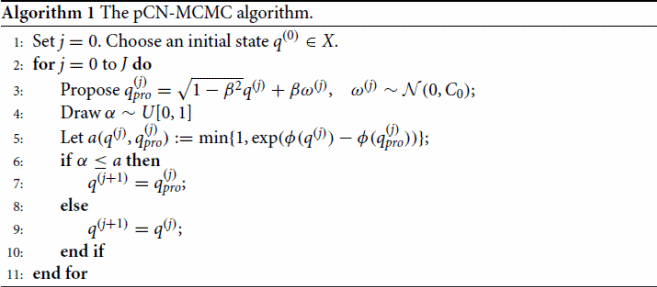
A kite-shaped obstacle: ${\mathrm{\Gamma }}_{kite}=(\cos \theta +0.65\cos 2\theta -0.65,1.5\sin \theta ),\theta \in [0,2\pi ).$In Figure 1, the conditioned mean estimates of the posterior distribution are displayed from full-aperture observations with noise levels $\delta =0.005,0.01,0.05$. From these numerical results, one can see that the proposed method is effective to recover the shape of the scatterer. Moreover, the data noise level is a crucial factor to the reconstructed results. It comes as no surprise that the reconstructed results are better with a smaller noise level δ. Fix the noise level $\delta =0.01$. We present the reconstructed results from different limited-aperture data in Figure 2. The results displayed in Figure 2 show the effect of the aperture of observations on the posterior distribution. The results of reconstruction deteriorate as the aperture gets smaller. Moreover, it is intuitive that the segment of the boundary of the scatterer closed to the location of given data can be captured well. Finally, some statistical information are presented. Without loss of generality, we show the Markov chains of the coefficients $a_0$, $a_1$ and $b_1$ in Figure 3 and omit the other coefficients. As shown in Figure 3, these results with different noise levels or different apertures suggest that these Markov chains can reach stability. 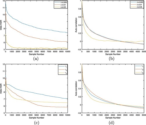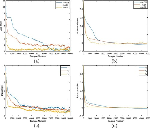Figure 4 shows the trace plots of the negative log-likelihood $\varphi \left(q\right)$ (or data-misfit) and the corresponding auto-correlation functions with different noise levels and different apertures, respectively. After a few iterations, it can be observed that the pCN can arrive at the stationary stage. The corresponding auto-correlation functions decay to zero.

Figure 1. Reconstruction for the kite-shaped scatterer with $\delta =0.005,0.01,0.05$.

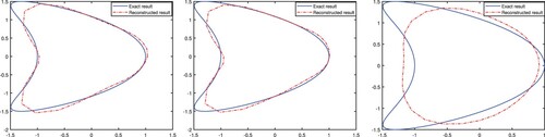
Figure 2. Reconstruction for the kite-shaped scatterer with ${\gamma }_1,{\gamma }_2,{\gamma }_3$, $\delta =0.01$.

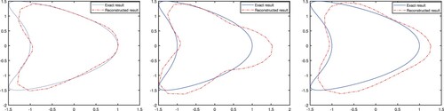
Figure 3. The first row denotes the Markov chains of the coefficients $a_0$, $a_1$ and $b_1$ with $\delta =0.005,0.01,0.05$. The second row denotes the Markov chains of the coefficients $a_0$, $a_1$ and $b_1$ with ${\gamma }_1,{\gamma }_2,{\gamma }_3$, $\delta =0.01$.

Figure 4. The traceplots of the negative log-likelihood $\varphi \left(q\right)$ and the corresponding auto-correlation functions for the kite-shaped scatterer, respectively.

Example 5.2

A pear-shaped obstacle: ${\mathrm{\Gamma }}_{pear}=\left(r\right(\theta )\cos \theta ,r(\theta )\sin \theta ),\theta \in [0,2\pi ),$where $r\left(\theta \right)=\frac{5+\sin 3\theta }{6}$. In Figure 5, we present the reconstructed results from full aperture data with noise level $\delta =0.005,0.01,0.05$. Obviously, the proposed method is effective to reconstruct the shape of the scatterer with different noise levels. When the data is polluted by a smaller noise level, the reconstructed result is better than that contaminated by a larger noise level. Figure 6 shows the reconstructed scatterer from different limited-aperture data. We find that the proposed method is also useful to recover the boundary of the scatterer from limited-aperture data. In Figure 7, the Markov chains of the coefficients $a_0$, $a_1$ and $b_1$ are displayed with different noise levels and different limited apertures, respectively. As shown in Figure 7, these chains can basically arrive at a stable. Figure 8 displays the traceplots of the negative log-likelihood $\varphi \left(q\right)$ and the corresponding auto-correlation functions, respectively. We can observe that the auto-correlation functions quickly decay to zero with larger noise level or smaller limited-aperture data.

Figure 5. Reconstruction for the pear-shaped scatterer with $\delta =0.005,0.01,0.05$.

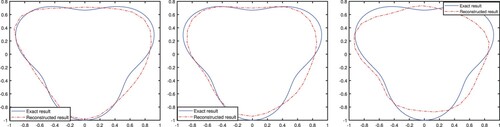
Figure 6. Reconstruction for the pear-shaped scatterer with ${\gamma }_1,{\gamma }_2,{\gamma }_3$, $\delta =0.01$.

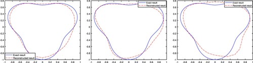
Figure 7. The first row denotes the Markov chains of the coefficients $a_0$, $a_1$ and $b_1$ with $\delta =0.005,0.01,0.05$. The second row denotes the Markov chains of the coefficients $a_0$, $a_1$ and $b_1$ with ${\gamma }_1,{\gamma }_2,{\gamma }_3$, $\delta =0.01$.

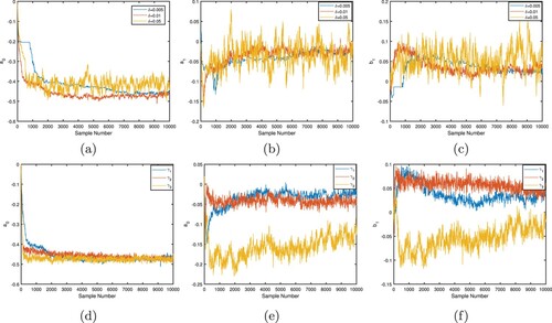
Figure 8. The traceplots of the negative log-likelihood $\varphi \left(q\right)$ and the corresponding auto-correlation functions for the pear-shaped scatterer, respectively.

6. Conclusion

In this work, we consider the Bayesian inference for reconstructing the shape of the scatterer. We choose the Gaussian measure as our prior and prove the well-posedness result for the posterior distribution. The numerical results show the effectiveness of the proposed method. In future work, we would like to use the variational Gaussian approximation instead of the sampling methods to extract the knowledge of the posterior distribution. Moreover, we can develop the Bayesian method for more complex models, such as transmission eigenvalue problems, elastic and electromagnetic scattering problems.

Acknowledgments

This work is supported by the National Natural Science Foundation of China under grants No.11771068 and No.11501087.

Disclosure statement

No potential conflict of interest was reported by the author(s).

Additional information

Funding

This work is supported by the National Natural Science Foundation of China under grants Nos. 11771068 and 11501087.

References

- Colton D, Kress R. Inverse acoustic and electromagnetic scattering theory. 2nd ed. Berlin: Springer-Verlag; 1998. (Applied mathematical sciences).
- Hohage T, Schormann C. A Newton-type method for a transmission problem in inverse scattering. Inverse Probl. 1998;14:1207–1227.
- Lee KM. Inverse transmission scattering problem via a Dirichlet-to-Neumann map. Eng Anal Bound Elem. 2019;101:214–220.
- Ghosh Roy DN, Warner J, Couchman LS, et al. Inverse obstacle transmission problem in acoustics. Inverse Probl. 1998;14:903–929.
- Colton D, Coyle J, Monk P. Recent developments in inverse acoustic scattering theory. SIAM Rev. 2000;42:369–414.
- Colton D, Kirsch A. A simple method for solving inverse scattering problems in the resonance region. Inverse Probl. 1996;12:383–393.
- Colton D, Piana M, Potthast R. A simple method using Morozov's discrepancy principle for solving inverse scattering problems. Inverse Probl. 1997;13:1477–1493.
- Yang J, Zhang B, Zhang R. A sampling method for the inverse transmission problem for periodic media. Inverse Probl. 2012;28:Article ID: 035004.
- Colton D, Haddar H, Piana M. The linear sampling method in inverse electromagnetic scattering theory. Inverse Probl. 2003;19:S105–S137.
- Dashti M, Stuart AM. The Bayesian approach to inverse problems. In: Handbook of uncertainty quantification. Cham: Springer; 2017.
- Kaipio JP, Somersalo E. Statistical and computational inverse problems. New York: Springer-Verlag; 2005. (Applied mathematical sciences).
- Stuart AM. Inverse problems: A Bayesian perspective. Acta Numer. 2010;5:451–559.
- Bui-Thanh T, Ghattas O. An analysis of infinite dimensional Bayesian inverse shape acoustic scattering and its numerical approximation. SIAM/ASA J Uncertain Quantification. 2014;2:203–222.
- Huang J, Deng Z, Xu L. Bayesian approach for inverse interior scattering problems with limited aperture. Appl Anal. 2020;1–14. https://doi.org/https://doi.org/10.1080/00036811.2020.1781828.
- Li Z, Deng Z, Sun J. Extended-sampling-Bayesian method for limited aperture inverse scattering problems. SIAM J Imag Sci. 2020;13:422–444.
- Li Z, Liu Y, Sun J, et al. Quality-Bayesian approach to inverse acoustic source problems with partial data. SIAM J Sci Comput. 2021;43:A1062–A1080.
- Liu J, Liu Y, Sun J. An inverse medium problem using Stekloff eigenvalues and a Bayesian approach. Inverse Probl. 2019;35:Article ID: 94004.
- Wang Y. Seismic inversion: theory and applications. Hoboken: John Wiley and Sons; 2016.
- Wang Y, Ma F, Zheng E. Bayesian method for shape reconstruction in the inverse interior scattering problem. Math Probl Eng. 2015;2:1–12.
- Bui-Thanh T, Ghattas O, Martin J, et al. A computational framework for infinite-dimensional Bayesian inverse problems part I: the linearized case, with application to global seismic inversion. SIAM J Sci Comput. 2013;35:A2494–A2523.
- Cui T, Law KJH, Marzouk YM. Dimension-independent likelihood-informed MCMC. J Comput Phys. 2016;304:109–137.
- Martin J, Wilcox LC, Burstedde C, et al. A stochastic Newton MCMC method for large-scale statistical inverse problems with application to seismic inversion. SIAM J Sci Comput. 2012;34:A1460–A1487.
- Petra N, Martin J, Stadler G, et al. A computational framework for infinite-dimensional Bayesian inverse problems, part II: Stochastic Newton MCMC with application to ice sheet flow inverse problems. SIAM J Sci Comput. 2014;36:A1525–A1555.
- Archambeau C, Cornford D, Opper M, et al. Gaussian process approximations of stochastic differential equations. In: JMLR: Workshop and Conference Proceedings, Bletchley Park, UK; 2007; 1:1–16.
- Arridge SR, Ito K, Jin B, et al. Variational Gaussian approximation for poisson data. Inverse Probl. 2018;34:Article ID: 025005.
- Challis E, Barber D. Gaussian Kullback-Leibler approximate inference. J Mach Learn Res. 2013;14:2239–2286.
- Cotter SL, Roberts GO, Stuart AM, et al. MCMC methods for functions: modifying old algorithms to make them faster. Statist Sci. 2012;28:424–446.
- Hsiao GC, Xu L. A system of boundary integral equations for the transmission problem in acoustics. Appl Numer Math. 2011;61:1017–1029.
- Hsiao GC, Wendland WL. Boundary integral equations. Berlin: Springer-Verlag; 2008.
- Hairer M. Introduction to stochastic PDEs. 2009. arXiv:0907.4178.