An inverse problem to simulate the transport of chloride in concrete by time–space fractional diffusion model

Abstract

In this paper, we proposed a fractional diffusion model to simulate the movement of chloride in concrete. In such complex porous structure some of the free chlorides, which are affected by the surrounding heterogeneous physical environment, will be bounded physically and chemically. Furthermore, experiments reveal that the interesting heavy-tailed phenomena appear in diffusion process. The time and spatial fractional derivatives are introduced to explain the anomalous diffusion and the dependence of medium properties. The numerical research shows that present model could better fit the experimental data and the diffusion of chloride in concrete is time-dependent and space-dependent.

Keywords:

• Fractional diffusion model
• bound chloride
• concrete corrosion
• complex porous medium
• finite differential method

2010 Mathematics Subject Classifications:

• 35K57
• 35R11
• 35R30
• 65M32

1. Introduction

The chloride penetration, which will bring about the steel corrosion in the concrete, is one of the crucial factors to destroy the persistence of concrete structures and bring about the attenuation of concrete service life [1–3]. In practical situation, the individual components used in concrete mixture, heterogeneous pore structure, combination and absorption of chloride ions, electrochemical reaction and many other factors will affect the transport of chloride in the concrete, and then Fick law may be not suitable to describe its movement. Furthermore, experiments also have confirmed that in saturated porous medium the random movement of the fluid particle will no longer satisfy Gaussian distribution [4,5]. Therefore, it is necessary for us to turn to new theories to detect the diffusion and reaction behaviours of chloride in concrete.

During the process of transport, besides the free chloride ($C_f$), the total chlorides ($C_T$) in concrete still include two parts: physically-bound chloride ($S_p$) and chemically-bound chloride ($S_c$) [6,7]. The introduction of bound chlorides into transport model can help us forecast the chloride entering more accurately. Early studies have shown that binding reactions occur in the diffusion process of free chloride ions [8–11], but the components of binding chloride have not been discussed clearly. Later, some experiments have revealed that C-S-H gels could adsorb some of free chloride ions, which would cause physical reaction, and the irreversible chemical combination also happened with other ions and substances [12–15].

In fact, concrete is a kind of heterogeneous and anisotropic complex porous medium, and according to pore diameter, its pores can be divided into three types: capillary pores, gel pores and stomata, where occurs reaction, diffusion, capillary suction and permeability [16]. Due to the anisotropy, heterogeneous and complexity of the medium property, many works have shown that the propagation of gas and liquid in concrete does not follow Fick law and Gaussian distribution [17–20]. Fractional derivative has been used to describe anomalous transport of many materials in porous media and complex environment, such as oil, biology, rock, hydrodynamics, rheology, viscoelasticity, electrical conduction of biological system, and so on [21–30]. A diffusion model with time fractional derivative has been constructed to simulate the transport of sodium chloride in a single crack and free chloride ions in concrete [31,32]. Furthermore, some semi-analytical and numerical methods have been used to solve this kind of diffusion equation [33,34]. The error and stability of the numerical method are also studied [34–38]. However, the chemical reaction and spatial characteristics of free chloride ions in pores have not been considered.

Motivated by above works, the fractional time–space diffusion model is proposed to simulate the transport of chloride in concrete. This paper is organized as follow: firstly we give the description of the establishment of fractional diffusion model. According to the discretization scheme in Section 3, the optimization algorithm based on modified hybrid Nelder–Mead simplex search and particle swarm optimization method (MH-NMSS- PSO) [39–42] is used to search for the unknown fractional derivative parameters to fit the experimental data in Section 4. Finally, the sensitivity analysis of different physical parameters in this problem is discussed.

2. Model description

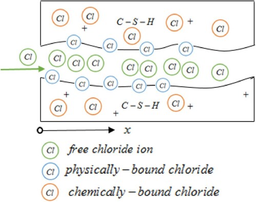
As shown in Figure 1, concrete is a complex heterogeneous porous material. Once the free chloride ions solution diffuse into it, chemical reaction will arise between some of them and cement pastes until the concentration of chemically-bound chlorides reach threshold at one position. The remaining free chlorides will move forth and some of them will adhere to the hole surface physically. The other free chloride ions will move forward again and maybe meet some holes unconnected each other, which induces the delay of the diffusion and results in the heavy-tailed phenomena [22]. Then the modified Fick law is introduced to describe the influence of time and space [7]: (1) ${\int }_0^t{\int }_0^{x}J(x^{\prime },\tau )\mathrm{d}{x}^{\prime }\mathrm{d}\tau =-{\int }_0^t{\int }_0^{x}k(x,x^{\prime };t,\tau )C_f(x^{\prime },\tau )\mathrm{d}{x}^{\prime }\mathrm{d}\tau ,$(1) where $C_f$ is the concentration of free chlorides and J is the flux. Here we assume that $k(x,x^{\prime };t,\tau )=k_x(x,x^{\prime })k_t(t,\tau )$.

Suppose the diffusion kernel function of space and time is negative power law function: (2) $k_x(x,x^{\prime })=\frac{D_e}{\epsilon \mathrm{\Gamma }(2-\beta )(x-x^{\prime }{)}^{\beta -1}},k_t(t,\tau )=\frac{1}{\mathrm{\Gamma }(\alpha )(t-\tau {)}^{1-\alpha }},$(2) where $D_e$ is the effective diffusion coefficient, ε is porosity.

Deriving x and t on both sides at the same time and according to the fractional derivative definition of Riemann–Liouville and Caputo [43–45], Equation (1(1) ${\int }_0^t{\int }_0^{x}J(x^{\prime },\tau )\mathrm{d}{x}^{\prime }\mathrm{d}\tau =-{\int }_0^t{\int }_0^{x}k(x,x^{\prime };t,\tau )C_f(x^{\prime },\tau )\mathrm{d}{x}^{\prime }\mathrm{d}\tau ,$(1) ) can be simplified as: (3) $J(x,t)=-\frac{D_e}{\epsilon }\frac{{\mathrm{\partial }}^{1-\alpha }}{\mathrm{\partial }{t}^{1-\alpha }}\frac{{\mathrm{\partial }}^{\beta -1}}{\mathrm{\partial }{x}^{\beta -1}}{C}_f(x,t),0<\alpha \le 1,1<\beta \le 2.$(3) The mass diffusion equation of chloride in concrete is [46]: (4) $\frac{\mathrm{\partial }{C}_T}{\mathrm{\partial }t}=-\mathrm{\nabla }\cdot J,$(4) where $C_T$ is the content of chloride ions. According to Refs. [14,47], the total ions are divided as three parts: (5) $C_T=C_f+S_p+S_c.$(5) In general, $S_c$ is a constant. The relationship between free chloride ions and physically-bound chloride satisfies the following linear binding isotherm [48]: $S_p=p{C}_f$, where p also is a constant.

Therefore, in order to balance the dimension, ${\lambda }_1$ and ${\lambda }_2$ are introduced to the mass diffusion equation, and then mass diffusion equation with fractional derivative can be written as: (6) ${\lambda }_1^{\alpha }\frac{{\mathrm{\partial }}^{\alpha }{C}_f(x,t)}{\mathrm{\partial }{t}^{\alpha }}={\lambda }_2^{\beta }\frac{D_e}{\epsilon (1+p)}\frac{{\mathrm{\partial }}^{\beta }{C}_f(x,t)}{\mathrm{\partial }{x}^{\beta }},$(6) where ${\lambda }_1$ and ${\lambda }_2$ are constants with dimensions $s^{1-1/\alpha }$ and $m{m}^{1-2/\beta }$, respectively.

It is assumed that there is no free chloride ions inside concrete at the beginning and the concentration of free chloride ion exposed to the external environment is $C_s$. Free chloride ions can migrate in the concrete continuously. In addition, the concentration and change of free chloride in deep position of concrete are very small. The initial and boundary conditions are (7) $\begin{array}{rl}& x\ge 0:C_f(x,t){|}_{t=0}=0,\end{array}$(7) (8) $\begin{array}{rl}& t>0:C_f(x,t){|}_{x=0}=C_s,C_f(x,t){|}_{x=+\mathrm{\infty }}=0.\end{array}$(8)

3. Numerical method

3.1. Difference scheme

To solve this problem, the diffusion equation is discretized. Let $x_i=ih,t_j=j\tau (i=0,1,2,\dots ,M,j=0,1,2,\dots ,N)$, where $(x_i,t_j)\in [0,X)\times [0,120]$ and X represents infinity, and $\tau =\frac{120}{N}$, $h=\frac{X}{M}$ are the time and space steps, respectively.

Theorem 1

When the time fractional order is $\alpha (0<\alpha <1),$ the time Caputo fractional derivative can be discretized into the difference scheme by L1 interpolation, as shown below [49]: (9) $\begin{array}{rl}\frac{{\mathrm{\partial }}^{\alpha }f(t_k)}{\mathrm{\partial }{t}^{\alpha }}& =\frac{{\tau }^{-\alpha }}{\mathrm{\Gamma }(2-\alpha )}\sum _{n=0}^{k-1}{a}_n^{(\alpha )}\left[f(t_{k-n})-f(t_{k-n-1})\right]+O({\tau }^{2-\alpha })\\ & =\frac{{\tau }^{-\alpha }}{\mathrm{\Gamma }(2-\alpha )}\left[a_0^{(\alpha )}f(t_k)-\sum _{n=1}^{k-1}\left(a_{k-n-1}^{(\alpha )}-a_{k-n}^{(\alpha )}\right)f(t_n)-a_{k-1}^{(\alpha )}f(t_0)\right]+O({\tau }^{2-\alpha }),\end{array}$(9) where the coefficient is expressed by $a_0^{(\alpha )}=1,a_n^{(\alpha )}=(n+1{)}^{1-\alpha }-n^{1-\alpha },n=1,2,\dots ,N$.

Theorem 2

When the order of the spatial fractional order is $\beta (1<\beta <2),$ the space Riemann–Liouville fractional derivative can be discretized by Grunwald–Letnikov algorithm as following [50]: (10) $\frac{{\mathrm{\partial }}^{\beta }}{\mathrm{\partial }{x}^{\beta }}C(x_i,t_{k+1})=\frac{1}{h^{\beta }}\sum _{j=0}^{i+1}{\omega }_j^{\beta }C(x_{i+1-j},t_{k+1})+O(h^s),$(10) In this formula, there are different forms of ${\omega }_j^{\beta }$ for different weight coefficient s. We select s as 1, and ${\omega }_j^{\beta }=(-1{)}^j\frac{\beta (\beta -1)\cdots (\beta -j+1)}{j!},(j=0,1,\dots )$.

According to Equations (9(9) $\begin{array}{rl}\frac{{\mathrm{\partial }}^{\alpha }f(t_k)}{\mathrm{\partial }{t}^{\alpha }}& =\frac{{\tau }^{-\alpha }}{\mathrm{\Gamma }(2-\alpha )}\sum _{n=0}^{k-1}{a}_n^{(\alpha )}\left[f(t_{k-n})-f(t_{k-n-1})\right]+O({\tau }^{2-\alpha })\\ & =\frac{{\tau }^{-\alpha }}{\mathrm{\Gamma }(2-\alpha )}\left[a_0^{(\alpha )}f(t_k)-\sum _{n=1}^{k-1}\left(a_{k-n-1}^{(\alpha )}-a_{k-n}^{(\alpha )}\right)f(t_n)-a_{k-1}^{(\alpha )}f(t_0)\right]+O({\tau }^{2-\alpha }),\end{array}$(9) ) and (10(10) $\frac{{\mathrm{\partial }}^{\beta }}{\mathrm{\partial }{x}^{\beta }}C(x_i,t_{k+1})=\frac{1}{h^{\beta }}\sum _{j=0}^{i+1}{\omega }_j^{\beta }C(x_{i+1-j},t_{k+1})+O(h^s),$(10) ), the following discretization format can be obtained: (11) $\begin{array}{rl}\frac{{\mathrm{\partial }}^{\alpha }{C_f}_i^j}{\mathrm{\partial }{\tau }^{\alpha }}& =\frac{{\tau }^{-\alpha }}{\mathrm{\Gamma }(2-\alpha )}\left[a_0^{(\alpha )}{C_f}_i^j-\sum _{n=1}^{j-1}(a_{j-n-1}^{(\alpha )}-a_{j-n}^{(\alpha )}){C_f}_i^n-a_{j-1}^{(\alpha )}{C_f}_i^0\right],\end{array}$(11) (12) $\begin{array}{rl}\frac{{\mathrm{\partial }}^{\beta }{C_f}_i^j}{\mathrm{\partial }{\eta }^{\beta }}& =\frac{1}{h^{\beta }}\sum _{k=0}^{i+1}{\omega }_k^{\beta }{C_f}_{i+1-k}^j.\end{array}$(12) Then the discretization scheme about mass diffusion equation with fractional derivative and initial boundary conditions can be written as: (13) $\begin{array}{rl}& {\lambda }_1^{\alpha }{r}_1\left[a_0^{(\alpha )}{C_f}_i^j-\sum _{n=1}^{j-1}(a_{j-n-1}^{(\alpha )}-a_{j-n}^{(\alpha )}){C_f}_i^n-a_{j-1}^{(\alpha )}{C_f}_i^0\right]={\lambda }_2^{\beta }\frac{D_e{r}_2}{\epsilon (1+p)}\sum _{k=0}^{i+1}{\omega }_k^{\beta }{C_f}_{i+1-k}^j,\end{array}$(13) (14) $\begin{array}{rl}& {C_f}_i^0=0,{C_f}_0^j=C_s,{C_f}_M^j=0,\end{array}$(14) where $r_1=\frac{{\tau }^{-\alpha }}{\mathrm{\Gamma }(2-\alpha )}$,$r_2=\frac{1}{h^{\beta }}$.

3.2. Existence and uniqueness of solutions

Lemma 1

The coefficients $a_j^{(\alpha )},$ ${\omega }_j^{\beta }(j=0,1,2,\dots )$ satisfy [45]:

1. $a_0^{(\alpha )}=1,a_j^{(\alpha )}>0,j=1,2,\dots ,$

2. $a_j^{(\alpha )}>a_{j+1}^{(\alpha )},j=0,1,\dots ,$

3. ${\omega }_0^{\beta }=1,{\omega }_1^{\beta }=-\beta <0,{\omega }_j^{\beta }>0,j=2,3,\dots ,$

4. $\sum _{j=0}^{\mathrm{\infty }}{\omega }_j^{\beta }=0$, and for $i=1,2,\dots$, we have $\sum _{j=0}^i{\omega }_j^{\beta }<0$.

Theorem 3

If the coefficient ${\omega }_j^{\beta }$ satisfies:

(1)

${\omega }_1^{\beta }=-\beta <0$, and ${\omega }_j^{\beta }>0$ when $j\ne 1$,

(2)

$\sum _{j=0}^{i+1}{\omega }_j^{\beta }\le 0$, then the solution of difference scheme (13(13) $\begin{array}{rl}& {\lambda }_1^{\alpha }{r}_1\left[a_0^{(\alpha )}{C_f}_i^j-\sum _{n=1}^{j-1}(a_{j-n-1}^{(\alpha )}-a_{j-n}^{(\alpha )}){C_f}_i^n-a_{j-1}^{(\alpha )}{C_f}_i^0\right]={\lambda }_2^{\beta }\frac{D_e{r}_2}{\epsilon (1+p)}\sum _{k=0}^{i+1}{\omega }_k^{\beta }{C_f}_{i+1-k}^j,\end{array}$(13) ) and (14(14) $\begin{array}{rl}& {C_f}_i^0=0,{C_f}_0^j=C_s,{C_f}_M^j=0,\end{array}$(14) ) exists and is unique.

Proof.

Difference scheme (13(13) $\begin{array}{rl}& {\lambda }_1^{\alpha }{r}_1\left[a_0^{(\alpha )}{C_f}_i^j-\sum _{n=1}^{j-1}(a_{j-n-1}^{(\alpha )}-a_{j-n}^{(\alpha )}){C_f}_i^n-a_{j-1}^{(\alpha )}{C_f}_i^0\right]={\lambda }_2^{\beta }\frac{D_e{r}_2}{\epsilon (1+p)}\sum _{k=0}^{i+1}{\omega }_k^{\beta }{C_f}_{i+1-k}^j,\end{array}$(13) ) can be rewritten as: (15) $\begin{array}{rl}{C_f}_i^j-r\sum _{k=0}^{i+1}{\omega }_k^{\beta }{C_f}_{i+1-k}^j& =a_{j-1}^{(\alpha )}{C_f}_i^0+\sum _{n=1}^{j-1}(a_{j-n-1}^{(\alpha )}-a_{j-n}^{(\alpha )}){C_f}_i^n,\\ & \times 1\le i\le M-1,1\le j\le N,\end{array}$(15) where $r={\displaystyle \frac{{\lambda }_2^{\beta }{D}_e{r}_2}{{\lambda }_1^{\alpha }{r}_1\epsilon (1+p)}}$.

For i = 0, the coefficient matrix A of Equations (14(14) $\begin{array}{rl}& {C_f}_i^0=0,{C_f}_0^j=C_s,{C_f}_M^j=0,\end{array}$(14) ) and (15(15) $\begin{array}{rl}{C_f}_i^j-r\sum _{k=0}^{i+1}{\omega }_k^{\beta }{C_f}_{i+1-k}^j& =a_{j-1}^{(\alpha )}{C_f}_i^0+\sum _{n=1}^{j-1}(a_{j-n-1}^{(\alpha )}-a_{j-n}^{(\alpha )}){C_f}_i^n,\\ & \times 1\le i\le M-1,1\le j\le N,\end{array}$(15) ) obeys $\sum _{l=1}^M|A_{0l}|=0<1=|A_{00}|$.

For i = M, $\sum _{l=0}^{M-1}|A_{Ml}|=0<1=|A_{MM}|$.

For $i\ne 0$ and $i\ne M$, according to conditions (1)–(2) and Lemma 1, we have $-r{\omega }_1^{\beta }=r\beta >r\sum _{k=0,k\ne 1}^{i+1}{\omega }_k^{\beta }>0$, that is, $|1-r{\omega }_1^{\beta }|=1-r{\omega }_1^{\beta }>r\sum _{k=0,k\ne 1}^{i+1}{\omega }_k^{\beta }$.

So coefficient matrix A is strictly diagonally dominant matrices. Matrix A is invertible, so the solution of the difference scheme (13(13) $\begin{array}{rl}& {\lambda }_1^{\alpha }{r}_1\left[a_0^{(\alpha )}{C_f}_i^j-\sum _{n=1}^{j-1}(a_{j-n-1}^{(\alpha )}-a_{j-n}^{(\alpha )}){C_f}_i^n-a_{j-1}^{(\alpha )}{C_f}_i^0\right]={\lambda }_2^{\beta }\frac{D_e{r}_2}{\epsilon (1+p)}\sum _{k=0}^{i+1}{\omega }_k^{\beta }{C_f}_{i+1-k}^j,\end{array}$(13) ) and (14(14) $\begin{array}{rl}& {C_f}_i^0=0,{C_f}_0^j=C_s,{C_f}_M^j=0,\end{array}$(14) ) exists and is unique.

3.3. Stability of the difference method

Next, we discuss the stability of the difference method.

Theorem 4

Assume ${C_f}_i^j$ is the numerical solution of Equations (13(13) $\begin{array}{rl}& {\lambda }_1^{\alpha }{r}_1\left[a_0^{(\alpha )}{C_f}_i^j-\sum _{n=1}^{j-1}(a_{j-n-1}^{(\alpha )}-a_{j-n}^{(\alpha )}){C_f}_i^n-a_{j-1}^{(\alpha )}{C_f}_i^0\right]={\lambda }_2^{\beta }\frac{D_e{r}_2}{\epsilon (1+p)}\sum _{k=0}^{i+1}{\omega }_k^{\beta }{C_f}_{i+1-k}^j,\end{array}$(13) ) and (14(14) $\begin{array}{rl}& {C_f}_i^0=0,{C_f}_0^j=C_s,{C_f}_M^j=0,\end{array}$(14) ), then (16) $||{{\mathit{C}}_{\mathit{f}}}^j|{|}_{\mathrm{\infty }}\le ||{{\mathit{C}}_{\mathit{f}}}^0|{|}_{\mathrm{\infty }},j=1,2,\dots .$(16)

Proof.

For j = 1, assume $||{{\mathit{C}}_{\mathit{f}}}^1|{|}_{\mathrm{\infty }}=|{C_f}_{i_0}^1|={max}_{0\le i\le M}|{C_f}_i^1|$. By Lemma 1, we have $\sum _{k=0}^{i_0+1}{\omega }_k^{\beta }<0$. Hence, $\begin{array}{rl}& ||{{\mathit{C}}_{\mathit{f}}}^1|{|}_{\mathrm{\infty }}=|{C_f}_{i_0}^1|\le |(1-r\sum _{k=0}^{i_0+1}{\omega }_k^{\beta }){C_f}_{i_0}^1|\\ & \le |{C_f}_{i_0}^1-r\sum _{k=0}^{i_0+1}{\omega }_k^{\beta }{C_f}_{i_0+1-k}^1|\\ & =|a_0^{(\alpha )}{C_f}_{i_0}^0|=|{C_f}_{i_0}^0|\\ & \le ||{{\mathit{C}}_{\mathit{f}}}^0||{}_{\mathrm{\infty }}\end{array}$For j = 2, assume $||{{\mathit{C}}_{\mathit{f}}}^2|{|}_{\mathrm{\infty }}=|{C_f}_{i_0}^2|={max}_{0\le i\le M}|{C_f}_i^2|$. By Lemma 1, we have $\sum _{k=0}^{i_0+1}{\omega }_k^{\beta }<0$. Hence, $\begin{array}{rl}& ||{{\mathit{C}}_{\mathit{f}}}^2|{|}_{\mathrm{\infty }}=|{C_f}_{i_0}^2|\le |(1-r\sum _{k=0}^{i_0+1}{\omega }_k^{\beta }){C_f}_{i_0}^2|\\ & \le |{C_f}_{i_0}^2-r\sum _{k=0}^{i_0+1}{\omega }_k^{\beta }{C_f}_{i_0+1-k}^2|\\ & =|a_1^{(\alpha )}{C_f}_{i_0}^0+(a_0^{(\alpha )}-a_1^{(\alpha )}){C_f}_{i_0}^1|\\ & \le a_1^{(\alpha )}|{C_f}_{i_0}^0|+(a_0^{(\alpha )}-a_1^{(\alpha )})|{C_f}_{i_0}^1|\\ & \le a_1^{(\alpha )}||{{\mathit{C}}_{\mathit{f}}}^0|{|}_{\mathrm{\infty }}+(a_0^{(\alpha )}-a_1^{(\alpha )})||{{\mathit{C}}_{\mathit{f}}}^1|{|}_{\mathrm{\infty }}\\ & \le a_1^{(\alpha )}||{{\mathit{C}}_{\mathit{f}}}^0|{|}_{\mathrm{\infty }}+(a_0^{(\alpha )}-a_1^{(\alpha )})||{{\mathit{C}}_{\mathit{f}}}^0|{|}_{\mathrm{\infty }}\\ & \le ||{{\mathit{C}}_{\mathit{f}}}^0||{}_{\mathrm{\infty }}\end{array}$For j>2, we prove similar to the above steps.

Suppose that $||{{\mathit{C}}_{\mathit{f}}}^j|{|}_{\mathrm{\infty }}=|{C_f}_{i_0}^j|={max}_{0\le i\le M}|{C_f}_i^j|$, then $\begin{array}{rl}& ||{{\mathit{C}}_{\mathit{f}}}^j|{|}_{\mathrm{\infty }}=|{C_f}_{i_0}^j|\le |(1-r\sum _{k=0}^{i_0+1}{\omega }_k^{\beta }){C_f}_{i_0}^j|\\ & \le |{C_f}_{i_0}^j-r\sum _{k=0}^{i_0+1}{\omega }_k^{\beta }{C_f}_{i_0+1-k}^j|=|a_{j-1}^{(\alpha )}{C_f}_{i_0}^0+\sum _{n=1}^{j-1}(a_{j-n-1}^{(\alpha )}-a_{j-n}^{(\alpha )}){C_f}_{i_0}^n|\\ & \le a_{j-1}^{(\alpha )}|{C_f}_{i_0}^0|+\sum _{n=1}^{j-1}(a_{j-n-1}^{(\alpha )}-a_{j-n}^{(\alpha )})|{C_f}_{i_0}^n|\\ & \le a_{j-1}^{(\alpha )}||{{\mathit{C}}_{\mathit{f}}}^0|{|}_{\mathrm{\infty }}+\sum _{n=1}^{j-1}(a_{j-n-1}^{(\alpha )}-a_{j-n}^{(\alpha )})\underset{1\le k\le j-1}{max}||{{\mathit{C}}_{\mathit{f}}}^k|{|}_{\mathrm{\infty }}\\ & \le a_{j-1}^{(\alpha )}||{{\mathit{C}}_{\mathit{f}}}^0|{|}_{\mathrm{\infty }}+\sum _{n=1}^{j-1}(a_{j-n-1}^{(\alpha )}-a_{j-n}^{(\alpha )})||{{\mathit{C}}_{\mathit{f}}}^0|{|}_{\mathrm{\infty }}\\ & =||{{\mathit{C}}_{\mathit{f}}}^0|{|}_{\mathrm{\infty }}\end{array}$Hence, Theorem 4 is proved.

Let ${\widetilde{C_f}}_i^j(i=0,1,\dots ,M;j=0,1,\dots ,N)$ be the approximate solution of Equation (15(15) $\begin{array}{rl}{C_f}_i^j-r\sum _{k=0}^{i+1}{\omega }_k^{\beta }{C_f}_{i+1-k}^j& =a_{j-1}^{(\alpha )}{C_f}_i^0+\sum _{n=1}^{j-1}(a_{j-n-1}^{(\alpha )}-a_{j-n}^{(\alpha )}){C_f}_i^n,\\ & \times 1\le i\le M-1,1\le j\le N,\end{array}$(15) ), the error $e_i^j={\widetilde{C_f}}_i^j-{C_f}_i^j(i=0,1,\dots ,M;j=0,1,\dots ,N)$ satisfies (17) $e_i^j-r\sum _{k=0}^{i+1}{\omega }_k^{\beta }{e}_{i+1-k}^j=a_{j-1}^{(\alpha )}{e}_i^0+\sum _{n=1}^{j-1}(a_{j-n-1}^{(\alpha )}-a_{j-n}^{(\alpha )})e_i^n.$(17) Apply Theorem 4, we obtain (18) $||{\mathit{E}}^{\mathit{j}}|{|}_{\mathrm{\infty }}\le ||{\mathit{E}}^{\mathbf{0}}|{|}_{\mathrm{\infty }},j=1,2,\dots ,N,$(18) where $||{\mathit{E}}^{\mathit{j}}|{|}_{\mathrm{\infty }}={max}_{0\le i\le M}|e_i^j|$. The following conclusion is obtained.

Theorem 5

The fractional implicit difference method of Equation (13(13) $\begin{array}{rl}& {\lambda }_1^{\alpha }{r}_1\left[a_0^{(\alpha )}{C_f}_i^j-\sum _{n=1}^{j-1}(a_{j-n-1}^{(\alpha )}-a_{j-n}^{(\alpha )}){C_f}_i^n-a_{j-1}^{(\alpha )}{C_f}_i^0\right]={\lambda }_2^{\beta }\frac{D_e{r}_2}{\epsilon (1+p)}\sum _{k=0}^{i+1}{\omega }_k^{\beta }{C_f}_{i+1-k}^j,\end{array}$(13) ) is unconditionally stable.

3.4. Convergence of difference method

The convergence of the difference scheme is discussed as follows.

Let $C_f(x_i,t_j)(i=1,2,\dots ,M-1;j=1,2,\dots ,N)$ be the exact solution of Equation (6(6) ${\lambda }_1^{\alpha }\frac{{\mathrm{\partial }}^{\alpha }{C}_f(x,t)}{\mathrm{\partial }{t}^{\alpha }}={\lambda }_2^{\beta }\frac{D_e}{\epsilon (1+p)}\frac{{\mathrm{\partial }}^{\beta }{C}_f(x,t)}{\mathrm{\partial }{x}^{\beta }},$(6) ) at point $(x_i,t_j)$. Then, (19) $C_f(x_i,t_j)-r\sum _{k=0}^{i+1}{\omega }_k^{\beta }{C}_f(x_{i+1-k},t_j)=a_{j-1}^{(\alpha )}{C}_f(x_i,t_0)+\sum _{n=1}^{j-1}(a_{j-n-1}^{(\alpha )}-a_{j-n}^{(\alpha )})C_f(x_i,t_n)+R_i^j,$(19) The error between the exact solution and the numerical solution is defined as ${\rho }_i^j=C_f(x_i,t_j)-{C_f}_i^j(i=1,2,\dots ,M-1;j=1,2,\dots ,N)$, ${\mathit{R}}^j=(R_1^j,R_2^j,\dots ,R_{M-1}^j{)}^T$, and subtract Equations (15(15) $\begin{array}{rl}{C_f}_i^j-r\sum _{k=0}^{i+1}{\omega }_k^{\beta }{C_f}_{i+1-k}^j& =a_{j-1}^{(\alpha )}{C_f}_i^0+\sum _{n=1}^{j-1}(a_{j-n-1}^{(\alpha )}-a_{j-n}^{(\alpha )}){C_f}_i^n,\\ & \times 1\le i\le M-1,1\le j\le N,\end{array}$(15) ) from (19(19) $C_f(x_i,t_j)-r\sum _{k=0}^{i+1}{\omega }_k^{\beta }{C}_f(x_{i+1-k},t_j)=a_{j-1}^{(\alpha )}{C}_f(x_i,t_0)+\sum _{n=1}^{j-1}(a_{j-n-1}^{(\alpha )}-a_{j-n}^{(\alpha )})C_f(x_i,t_n)+R_i^j,$(19) ), we obtain (20) $\begin{array}{rl}& {\rho }_i^j-r\sum _{k=0}^{i+1}{\omega }_k^{\beta }{\rho }_{i+1-k}^j=a_{j-1}^{(\alpha )}{\rho }_i^0+\sum _{n=1}^{j-1}(a_{j-n-1}^{(\alpha )}-a_{j-n}^{(\alpha )}){\rho }_i^n+R_i^j,\\ & \times 1\le i\le M-1,1\le j\le N,\end{array}$(20) with initial and boundary conditions (21) $\begin{array}{rl}& {\rho }_i^0=0,i=0,1,\dots ,M,\end{array}$(21) (22) $\begin{array}{rl}& {\rho }_0^j={\rho }_M^j=0,j=0,1,\dots ,N,\end{array}$(22) where truncation error $R_i^j$ satisfies $|R_i^j|\le C{\tau }^{\alpha }({\tau }^{2-\alpha }+h)$, and C is a positive constant.

Proposition 1

$||{\mathit{Y}}^j|{|}_{\mathrm{\infty }}\le \overline{C}{\tau }^{\alpha }({\tau }^{2-\alpha }+h),$ where ${\mathit{Y}}^j=({\rho }_1^j,{\rho }_2^j\cdots {\rho }_{M-1}^j)$, $||{\mathit{Y}}^j|{|}_{\mathrm{\infty }}={max}_{1\le i\le M-1}|{\rho }_i^j|$ and $\overline{C}$ is a constant.

Proof.

Similar to the proof of stability. For j = 1, assume $||Y^1|{|}_{\mathrm{\infty }}=|{\rho }_{i_0}^1|={max}_{0\le i\le M}|{\rho }_i^1|$. Hence, $\begin{array}{rl}& ||{\mathit{Y}}^1|{|}_{\mathrm{\infty }}=|{\rho }_{i_0}^1|\le |(1-r\sum _{k=0}^{i_0+1}{\omega }_k^{\beta }){\rho }_{i_0}^1|\\ & \le |{\rho }_{i_0}^1-r\sum _{k=0}^{i_0+1}{\omega }_k^{\beta }{\rho }_{i_0+1-k}^1|=|a_0^{(\alpha )}{\rho }_{i_0}^0+R_{i_0}^j|=|{\rho }_{i_0}^0+R_{i_0}^1|\\ & \le C_1{\tau }^{\alpha }({\tau }^{2-\alpha }+h).\end{array}$Thus, $||{\mathit{Y}}^1|{|}_{\mathrm{\infty }}\le C_1(a_0^{(\alpha )}{)}^{-1}{\tau }^{\alpha }({\tau }^{2-\alpha }+h)$.

For j>1, using $(a_j^{(\alpha )}{)}^{-1}\ge (a_k^{(\alpha )}{)}^{-1}(k=0,1,\dots ,j)$, we prove similar to the above steps. $\begin{array}{rl}||{\mathit{Y}}^j|{|}_{\mathrm{\infty }}& =|{\rho }_{i_0}^j|\le |(1-r\sum _{k=0}^{i_0+1}{\omega }_k^{\beta }){\rho }_{i_0}^j|\\ & \le |{\rho }_{i_0}^j-r\sum _{k=0}^{i_0+1}{\omega }_k^{\beta }{\rho }_{i_0+1-k}^j|=|a_{j-1}^{(\alpha )}{\rho }_{i_0}^0+\sum _{n=1}^{j-1}(a_{j-n-1}^{(\alpha )}-a_{j-n}^{(\alpha )}){\rho }_{i_0}^n+R_{i_0}^j|\\ & \le \sum _{n=1}^{j-1}(a_{j-n-1}^{(\alpha )}-a_{j-n}^{(\alpha )})|{\rho }_{i_0}^n|+C_1{\tau }^{\alpha }({\tau }^{2-\alpha }+h)\\ & \le \left[a_{j-1}^{(\alpha )}+\sum _{n=1}^{j-1}(a_{j-n-1}^{(\alpha )}-a_{j-n}^{(\alpha )})\right](a_{j-1}^{(\alpha )}{)}^{-1}{C}_1{\tau }^{\alpha }({\tau }^{2-\alpha }+h)\\ & =C_1(a_{j-1}^{(\alpha )}{)}^{-1}{\tau }^{\alpha }({\tau }^{2-\alpha }+h).\end{array}$Because ${lim}_{j\to \mathrm{\infty }}{\displaystyle \frac{{(a_j^{(\alpha )})}^{-1}}{j^{\alpha }}=\underset{j\to \mathrm{\infty }}{lim}{\displaystyle \frac{j^{-\alpha }}{{(j+1)}^{1-\alpha }-j^{1-\alpha }}=\underset{j\to \mathrm{\infty }}{lim}{\displaystyle \frac{j^{-1}}{{(1+\frac{1}{j})}^{1-\alpha }-1}=\underset{j\to \mathrm{\infty }}{lim}{\displaystyle \frac{j^{-1}}{(1-\alpha )j^{-1}}={\displaystyle \frac{1}{1-\alpha }}}}}}$, there exists a constant $C_2$ for which $||{\mathit{Y}}^j|{|}_{\mathrm{\infty }}\le C_2{j}^{\alpha }{\tau }^{\alpha }({\tau }^{2-\alpha }+h)$.

Furthermore, $j\tau$ is finite, the following theorem is proved.

Theorem 6

Let ${C_f}_i^j$ be the numerical solution of Equation (13(13) $\begin{array}{rl}& {\lambda }_1^{\alpha }{r}_1\left[a_0^{(\alpha )}{C_f}_i^j-\sum _{n=1}^{j-1}(a_{j-n-1}^{(\alpha )}-a_{j-n}^{(\alpha )}){C_f}_i^n-a_{j-1}^{(\alpha )}{C_f}_i^0\right]={\lambda }_2^{\beta }\frac{D_e{r}_2}{\epsilon (1+p)}\sum _{k=0}^{i+1}{\omega }_k^{\beta }{C_f}_{i+1-k}^j,\end{array}$(13) ), and $C_f(x_i,t_j)$ is the exact solution of Equation (6(6) ${\lambda }_1^{\alpha }\frac{{\mathrm{\partial }}^{\alpha }{C}_f(x,t)}{\mathrm{\partial }{t}^{\alpha }}={\lambda }_2^{\beta }\frac{D_e}{\epsilon (1+p)}\frac{{\mathrm{\partial }}^{\beta }{C}_f(x,t)}{\mathrm{\partial }{x}^{\beta }},$(6) ) at point $(x_i,t_j)$. Then exists a constant $C_3$ for which (23) $|{C_f}_i^j-C_f(x_i,t_j)|\le C_3({\tau }^{2-\alpha }+h),1\le i\le M-1,1\le j\le N.$(23)

4. Parameters estimation

Here MH-NMSS-PSO- is used to estimate the unknown parameters α, β, ${\lambda }_1$, ${\lambda }_2$ to satisfy the experimental data. This method, which is proposed by Fan [51] and extended by Liu [50,52,53], is a combination of NMSS and PSO, and can find the global optimum with faster convergence speed. Furthermore, it does not need the derivatives of the function under exploration [51]. Let $(\alpha ,\beta ,{\lambda }_1,{\lambda }_2)=(p_1,p_2,p_3,p_4)\in R^4$, where $(\alpha ,\beta ,{\lambda }_1,{\lambda }_2)\in [0,1]\times [1,2]\times (0,1]\times (0,1]$.

Here we assume that the numerical solutions for Equations (13(13) $\begin{array}{rl}& {\lambda }_1^{\alpha }{r}_1\left[a_0^{(\alpha )}{C_f}_i^j-\sum _{n=1}^{j-1}(a_{j-n-1}^{(\alpha )}-a_{j-n}^{(\alpha )}){C_f}_i^n-a_{j-1}^{(\alpha )}{C_f}_i^0\right]={\lambda }_2^{\beta }\frac{D_e{r}_2}{\epsilon (1+p)}\sum _{k=0}^{i+1}{\omega }_k^{\beta }{C_f}_{i+1-k}^j,\end{array}$(13) ) and (14(14) $\begin{array}{rl}& {C_f}_i^0=0,{C_f}_0^j=C_s,{C_f}_M^j=0,\end{array}$(14) ) at the point of $P=(p_1,p_2,p_3,p_4)$ could have best agreement with the experimental data [54]. The better point can be evaluated until the stop condition is satisfied [55]: (24) $g(P^{\ast })=g_{min}=\underset{P\in R^4}{min}g(P)=\underset{P\in R^4}{min}\sqrt{\sum _{j=0}^N\frac{{(C_f(t_j)-{C_f}^j)}^2}{N+1}}$(24) where $C_f(t_j)$ is the experimental data in the time of $t_j$, ${C_f}^j$ is the numerical solution at time $t_j$, and N is the number of experimental data. Therefore, the parameters of four variables can be estimated by MH-NMSS-PSO, which is summarized in Algorithm 1.

In MH-NMSS-PSO- algorithm, $3m$ particles is initialized: $P_i=(p_{1,i},p_{2,i},\dots ,p_{m,i}),i=1,2,\dots ,3m$, where $p_{j,i}$ is the value of parameter $p_j(j=1,2\cdots ,m)$ and is expressed with a random number $Rand\in (0,1)$ as: (25) $p_{j,i}=p_j^{(min)}+Rand\times (p_j^{(max)}-p_j^{(min)}),i=1,2,\dots ,3m+1;j=1,2,\dots ,m.$(25) The initial velocity of $2m$ particles in PSO is defined as: (26) $V_{j,i}=(V_j^{(max)}-V_j^{(min)})/L_j,i=m+2,\dots ,3m+1;j=1,2,\dots ,m$(26) where $L_j$ is an integer, m is the number of unknown variables.

And velocities and positions of particles in PSO algorithm is updated by: (27) $\begin{array}{r}\begin{array}{rl}{V}_{j,i}^{\mathrm{new}}& =w\times V_{j,i}^{\mathrm{old}}+C_1\times {\mathrm{Rand}}_1\times \left(P{b}_{j,i}-P_{j,i}^{\mathrm{old}}\right)+C_2\times \mathrm{Rand}{}_2\times \left(P{g}_j-P_{j,i}^{\mathrm{old}}\right)\\ P_{j,i}^{\mathrm{new}}& =P_{j,i}^{\mathrm{old}}+V_{j,i}^{\mathrm{new}},j=1,2,\dots ,m;i=m+2,\dots ,3m+1\end{array}\end{array}$(27) where $w,C_1$ and $C_2$ are coefficients given by Fan et al. [51].

In addition, stop condition is added as the number of iteration has not reach the maximum number of iterations: (28) $S={\left[\sum _{i=1}^{m+1}\frac{{\left(\overline{g}-\sqrt{g_i}\right)}^2}{m+1}\right]}^{1/2}<\overline{\epsilon }$(28) where $g_i^{\ast }=g(P_i)=\sqrt{g_i}=\sqrt{g_i(p_{1,i},p_{2,i},\dots ,p_{m,i})},\overline{g}=\sum _{i=1}^{m+1}\frac{g_i^{\ast }}{m+1}$ and $\overline{\epsilon }$ is a settled minimum value.

Figure 1. Schematic diagram of chlorides diffusion in concrete. 

5. Results and sensitivity analysis of parameters

Based on above discretization scheme and optimization algorithm, the correctness of fractional diffusion model is proved by experimental data from ordinary Portland cement (OPC) concrete, fly ash (FA) concrete and ground blast furnace (Slag) concrete [14,54], which is shown in Figure 2 and Table 1. Since concrete interior is full of aggregates and pores with different sizes, it is possible for the aggregates to block the pores. All of these make the diffusion to be spatial dependence. Furthermore, the values of parameters estimated in Table 1 also reveal that the surrounding environment has important influence on the transport of chloride in the concrete. In addition, the simulation result for the FA35-40 show that the diffusion is time-dependence. When maximum number of iterations is set to 500, the CPU time and the convergence rate for searching the global optimal parameters on a personal laptop with Intel(R) Core(TM) i5-5200U CPU is showed in Table 2.

Figure 2. The experimental data compared with present model.  

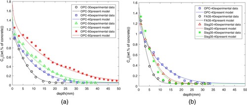
Table 1. The estimated parameters according to related parameters from Ref. [54].

concrete	$C_s$	$D_e$	ε	α	β	${\lambda }_1$	${\lambda }_2$
OPC-30	0.89031	0.04579	0.123	1.00000	1.98043	1	0.86691
OPC-40	1.06521	0.12096	0.145	1.00000	1.88568	1	0.97801
OPC-50	1.13956	0.20736	0.153	1.00000	1.89366	1	0.93214
OPC-60	1.35490	0.45792	0.179	1.00000	1.88595	1	1.00000
FA35-40	1.16886	0.02592	0.157	0.88945	2.00000	0.95562	1
Slag20-40	1.04577	0.06566	0.142	1.00000	1.97989	1	0.87744
Slag35-40	1.02538	0.0432	0.139	1.00000	2.00000	1	1

Table 2. Convergence rate and CPU time of OPC-30 for the process of searching optimal parameters.

$\overline{\epsilon }$	τ (day)	Iterations	Standard error	CPU time (s)
0.05	1	3	0.0418	40
0.025	1	5	0.0238	62
0.0151	1	7	0.0143	98
0.0151	5	11	0.0147	22
0.0151	10	19	0.0150	15

The influence of parameters on chloride diffusion in the OPC concrete with OPC 30 is shown in Figures 3–7. Figure 3(a) and (b) illustrates the distribution of chloride content in concrete at different depths and time. Once the diffusion begins, the concentration of chemically bound chloride reaches the saturation value immediately. With time going on, the chloride concentration will grow up and the diffusion will continue to move towards the depth of concrete. What's more, with the accumulation of physically-bound chloride, the total chloride concentration at the same depth also increases with the increasing time. In terms of diffusion rate, compared with the content at initial position, the total content of chloride will decrease because the free chloride ions will decrease with the increasing depth.

Figure 3. Influence of  t and depth on the chloride diffusion.

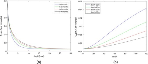
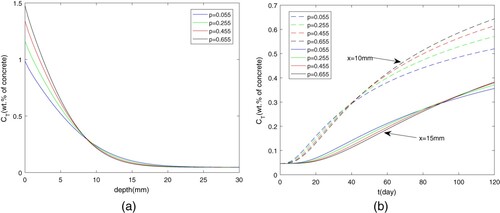
Figure 4(a) and (b) illustrates the effect of p on chloride diffusion. Figure 4(a) gives the total chloride ions distribution as time is 120 s. Since at the entrance the content of free chloride ions is a constant, the increasing p mean that much more chloride ions are absorbed on the pores at the initial position and during transport process. This leads to the dramatic change of the $C_T$ at the initial stage. Figure 4(b) depicts the distribution of chloride content at depths of 10 mm and 15 mm, respectively. On the whole, with the increasing time, the total chloride ions will be higher since the chloride ions are absorbed on the pores firstly near the entrance. Furthermore, the higher adsorption capacity means that chloride ions will be more easy to accumulate at the same place, and this also leads to higher $C_T$ as time is long enough.

Figure 4. Influence of p on the chloride diffusion. 

The impact of initial concentration $C_s$ and porosity ε on chloride diffusion is shown in Figures 5 and 6. It is very easy to explain that higher initial concentration of free chloride will result in the higher $C_T$ at the same place or the same time. The reduction of porosity coefficient means that there are many more pores to absorb the chloride ions, which cause the increase of $C_T$.

Figure 5. Influence of  Cs on the chloride diffusion.  

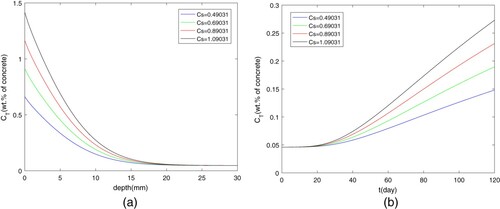
Figure 6. Influence of ϵ on the chloride diffusion. 

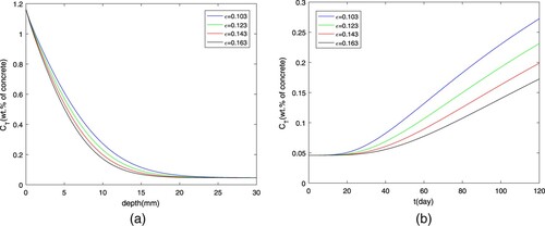
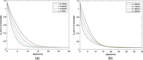
Figure 7 illustrates the effects of fractional derivatives on chloride diffusion in concrete. As shown in Figure 7(a), at the same diffusion depth, the smaller α is, the less chloride concentration is. As shown in Figure 7(b), the impact of β on diffusion has two sides. The increase of fractional derivative is beneficial to the accumulation of $C_T$ in front of the intersection and the influence degree is more obvious, while the opposite is true after the intersection. It also reveals that the spatial fractional derivative can reflect the nonlocality of diffusion. In a word, fractional order can describe the diffusion of materials in porous complex media well, which is consistent with the characteristics of time dependence and spatial nonlocality.

Figure 7. Influence of fractional derivatives on the chloride diffusion. 

6. Conclusions

This study presents a time-space fractional model to describe the transport of chloride ions in seven different types of concrete. It is noteworthy that free chloride ions are presented in three forms in concrete due to reaction, and the impact of porosity on diffusion is taken into account. The fitting results also show that the time fractional order α and the space fractional order β can explain spatial nonlocality well. What's more, the finite difference method and the optimization algorithm can be applied to the similar fractional problems and to find the optimal value.

Acknowledgements

The work is supported by National Natural Science Foundation of China (No. 12072024), the Fundamental Research Funds for the Central Universities.

Disclosure statement

No potential conflict of interest was reported by the author(s).

Additional information

Funding

The work is supported by National Natural Science Foundation of China (No. 12072024), the Fundamental Research Funds for the Central Universities.

References

- Jau W-C, Tsay D-S. A study of the basic engineering properties of slag cement concrete and its resistance to seawater corrosion. Cem Concr Res. 1998;28(10):1363–1371.
- Angst U, Elsener B, Larsen CK, et al. Critical chloride content in reinforced concrete – a review. Cem Concr Res. 2009;39(12):1122–1138.
- Alonso C, Andrade C, Castellote M, et al. Chloride threshold values to depassivate reinforcing bars embedded in a standardized OPC mortar. Cem Concr Res. 2000;30(7):1047–1055.
- Liu Y, Teng Y, Lu G, et al. Experimental study on CO 2 diffusion in bulk n-decane and n-decane saturated porous media using micro-CT. Fluid Phase Equil. 2016;417:212–219.
- Sun D, Englezos P. Storage of CO2 in a partially water saturated porous medium at gashydrate formation conditions. Int J Greenh Gas Control. 2014;25:1–8.
- Baroghel-Bouny V, Wang X, Thiery M, et al. Prediction of chloride binding isotherms of cementitious materials by analytical model or numerical inverse analysis. Cem Concr Res. 2012;42(9):1207–1224.
- Li D, Li L, Wang X. Chloride diffusion model for concrete in marine environment with considering binding effect. Mar Struct. 2019;66:44–51.
- Glass G, Buenfeld N. The influence of chloride binding on the chloride induced corrosion risk in reinforced concrete. Corrosion Sci. 2000;42(2):329–344.
- Samson E, Marchand J. Numerical solution of the extended Nernst–Planck model. J Colloid Interface Sci. 1999;215(1):1–8.
- Jensen O, Hansen P, Coats A, et al. Chloride ingress in cement paste and mortar. Cem Concr Res. 1999;29(9):1497–1504.
- Page CL, Vennesland Ø. Pore solution composition and chloride binding capacity of silica fume cement pastes. Mat Constr. 1983;16(1):19–25.
- Loser R, Lothenbach B, Leemann A, et al. Chloride resistance of concrete and its binding capacity–comparison between experimental results and thermodynamic modeling. Cem Concr Compos. 2010;32(1):34–42.
- Geng J, Easterbrook D, Li L, et al. The stability of bound chlorides in cement paste with sulfate attack. Cem Concr Res. 2015;68:211–222.
- Li D, Wang X, Li L. An analytical solution for chloride diffusion in concrete with considering binding effect. Ocean Eng. 2019;191:106549.
- Song Q, Yu R, Shui Z, et al. Physical and chemical coupling effect of metakaolin induced chloride trapping capacity variation for Ultra High Performance Fibre Reinforced Concrete (UHPFRC). Constr Build Mater. 2019;223:765–774.
- Mohammed MK, Dawson AR, Thom NH. Macro/micro-pore structure characteristics and the chloride penetration of self-compacting concrete incorporating different types of filler and mineral admixture. Constr Build Mater. 2014;72:83–93.
- Auriault J, Lewandowska J. Non-gaussian diffusion modeling in composite porous media by homogenization: tail effect. Trans Porous Media. 1995;21(1):47–70.
- Kosakowski G. Anomalous transport of colloids and solutes in a shear zone. J Contam Hydrol. 2004;72(1):23–46.
- Gimmi T, Flühler H, Studer B, et al. Transport of volatile chlorinated hydrocarbons in unsaturated aggregated media. Water Air Soil Pollut. 1993;68(1):291–305.
- Nicholson C, Phillips JM. Ion diffusion modified by tortuosity and volume fraction in the extracellular microenvironment of the rat cerebellum. J Physiol. 1981;321(1):225–257.
- Sokolov IM, Klafter J. Field-induced dispersion in subdiffusion. Phys Rev Lett. 2006;97(14):140602.
- Chang A, Sun H, Zheng C, et al. A time fractional convection–diffusion equation to model gas transport through heterogeneous soil and gas reservoirs. Physica A. 2018;502:356–369.
- Magin RL, Ingo C, Colon-Perez L, et al. Characterization of anomalous diffusion in porous biological tissues using fractional order derivatives and entropy. Micropor Mesopor Mat. 2013;178:39–43.
- Nicholson C. Diffusion and related transportmechanisms in brain tissue. Rep Prog Phys. 2001;64(7):815–884.
- Suzuki A, Fomin SA, Chugunov VA, et al. Fractional diffusion modeling of heat transfer in porous and fractured media. Int J Heat Mass Transf. 2016;103:611–618.
- Obembe AD, Hossain ME, Abu-Khamsin SA. Variable-order derivative time fractional diffusion model for heterogeneous porous media. J Pet Sci Eng. 2017;152:391–405.
- Zhou HW, Yang S. Fractional derivative approach to non-Darcian flow in porous media. J Hydrol. 2018;566:910–918.
- Jiang X, Xu M, Qi H. The fractional diffusion model with an absorption term and modified Fick's law for non-local transport processes. Nonlinear Anal Real World Appl. 2010;11(1):262–269.
- Zhokh A, Strizhak P. Macroscale modeling the methanol anomalous transport in the porous pellet using the time-fractional diffusion and fractional brownian motion: A model comparison. Commun Nonlinear Sci Numer Simul. 2019;79:104922.
- Benson DA, Meerschaert MM, Revielle J. Fractional calculus in hydrologic modeling: a numerical perspective. Adv Water Resour. 2013;51:479–497. 35th Year Anniversary Issue.
- Sun H, Wang Y, Qian J, et al. An investigation on the fractional derivative model in characterizing sodium chloride transport in a single fracture. Eur Phys J Plus. 2019;134(9):440.
- Wei S, Chen W, Zhang J. Time-fractional derivative model for chloride ions sub-diffusion in reinforced concrete. Eur J Environ Civ Eng. 2015;21(3):319–331.
- Nawaz R, Khattak A, Akbar M, et al. Solution of fractional-order integro-differential equations using optimal homotopy asymptotic method. J Therm Anal Calor. 2020;6. DOI:https://doi.org/10.1007/s10973-020-09935-x.
- Akbar M, Nawaz R, Ahsan S, et al. New approach to approximate the solution of system of fractional order Volterra integro-differential equations. Res Phys. 2020;19:103453.
- Abbaszadeh M, Mehdi D. Numerical and analytical investigations for solving the inverse tempered fractional diffusion equation via interpolating element-free Galerkin (IEFG) method. J Therm Anal Calor. 2020;143:1917–1933.
- Abbaszadeh M. Error estimate of second-order finite difference scheme for solving the Riesz space distributed-order diffusion equation. Appl Math Lett. 2019;88:179–185.
- Abbaszadeh M, Dehghan M. Numerical investigation of reproducing kernel particle Galerkin method for solving fractional modified distributed-order anomalous sub-diffusion equation with error estimation. Appl Math Comput. 2021;392:125718.
- Abbaszadeh M, Dehghan M, Navon LM. A POD reduced-order model based on spectral Galerkin method for solving the space-fractional Gray-Scott model with error estimate. Appl Math Comput. 2020;1:1–24.
- Zahara E, Kao YT. Hybrid Nelder-Mead simplex search and particle swarm optimization for constrained engineering design problems. Expert Syst Appl. 2009;36(2):3880–3886.
- Vakil Baghmisheh MT, Peimani M, Sadeghi MH, et al. A hybrid particle swarm-Nelder-Mead optimization method for crack detection in cantilever beams. Appl Soft Comput. 2012;12(8):2217–2226.
- Mesbahi T, Khenfri F, Rizoug N, et al. Dynamical modeling of li-ion batteries for electric vehicle applications based on hybrid particle Swarm-Nelder-Mead (PSO-NM) optimization algorithm. Electr Power Syst Res. 2016;131:195–204.
- Begambre O, Laier J. A hybrid particle swarm optimization – simplex algorithm (PSOS) for structural damage identification. Adv Eng Softw. 2009;40(9):883–891.
- Podlubny I. Fractional differential equations: an introduction to fractional derivatives, fractional differential equations, to methods of their solution and some of their applications. Academic Press; San Diego; 1999.
- Samko SG, Kilbas AA, Marichev OI, et al. Fractional integrals and derivatives. Vol. 1, Yverdon Yverdon-les-Bains, Switzerland: Gordon and Breach Science Publishers; 1993.
- Liu F, Zhuang P, Anh V, et al. Stability and convergence of the difference methods for the space–time fractional advection–diffusion equation. Appl Math Comput. 2007;191(1):12–20.
- Yu B, Jiang X. A fractional anomalous diffusion model and numerical simulation for sodium ion transport in the intestinal wall. Adv Math Phys. 2013;2013:1–8.
- Glass GK, Buenfeld NR. The presentation of the chloride threshold level for corrosion of steel in concrete. Corros Sci. 1997;39(5):1001–1013.
- Li J, Shao W. The effect of chloride binding on the predicted service life of RC pipe piles exposed to marine environments. Ocean Eng. 2014;88:55–62.
- Chen R, Liu F, Anh V. Numerical methods and analysis for a multi-term time–space variable-order fractional advection–diffusion equations and applications. J Comput Appl Math. 2018;352:437–452.
- Liu F, Zhuang P, Burrage K. Numerical methods and analysis for a class of fractional advection–dispersion models. Comput Math Appl. 2012;64(10):2990–3007.
- Fan SS, Liang Y, Zahara E. Hybrid simplex search and particle swarm optimization for the global optimization of multimodal functions. Eng Optimiz. 2004;36(4):401–418.
- Liu F, Burrage K. Novel techniques in parameter estimation for fractional dynamical models arising from biological systems. Comput Math Appl. 2011;62(3):822–833.
- Qin S, Liu F, Turner I, et al. Multi-term time-fractional Bloch equations and application in magnetic resonance imaging. J Comput Appl Math. 2017;319:308–319.
- Qiao C, Ni W, Wang Q, et al. Chloride diffusion and wicking in concrete exposed to NaCl and mgCl 2 solutions. J Mater Civ Eng. 2018;30(3):04018015.
- Liu F, Burrage K, Hamilton NA. Some novel techniques of parameter estimation for dynamical models in biological systems. IMA J Appl Math. 2013;78(2):235–260.