A locally sequential refinement of the growth dynamics identification

Abstract

The approach is developed to specify a reconstruction of complicated functions using samples of limited size with invariant properties regarding the desired parameters. The idea is based on solutions to inverse problems, which should identify various representations of unknown parameters of a mathematical model and do so in a series. The sequential solutions to inverse problems ensure the identifiability of desired parameters that belong to an invariant family. The locally sequential refinement restricts local spikes additionally to the general regularization under a scheme of separate matching with observations. A simulation with inverse problems is applied to refine the known features of population dynamics. The reconstruction shows that the parameters of the Verhulst equation should be introduced as oscillatory functions. Based on the novel functional representation of the Verhulst equation parameters, the patterns of the COVID-19 spread and its progression in a given region are determined. The results emphasize the Verhulst equation’s character as a generalized and fruitful model for an object growth simulation.

KEYWORDS:

• Simulation
• parameter estimation
• identifiability
• regularization
• locally sequential refinement

Subject classifications codes:

• 34A34
• 34A55
• 47A52,65L09
• 65J20,65L08,65R30
• 65N21

1. Introduction

In practice, an object under examination often has features that require complicated functions for its mathematical representation. In turn, a complicated function necessitates an approximation basis of large volume, while samples used for the reconstruction of the desired quantities often have a small size. Because of this, solution stabilization is a crucial question, and a stable reconstruction of a large number of unknowns with a small size of samples is the actual theoretical and practical problem. The development of a suitable restriction approach is motivated by the fact that the function’s particularism facilitates determining essential regularities of the object in question.

The classical problem of determining essential details of functions by a sample with limited volume has many mathematical aspects [1–6]. The present investigation considers the reconstruction of complicated functions in detail, whose behavior and features are implicitly manifested by a discrete sample of a direct problem solution depending parametrically on sought object properties. Such a formulation necessitates a satisfactory approximation of the parameters of a given model, whose state should approximate a given discrete sample within known observation errors. The solution is sought within the constraint that the desired functions require a large-size approximate basis, while, the small-size basis is sufficient to describe initial data and given sample adequately. The method of the stable extension of an approximation basis of sought quantities without a significant amount of additional information and observations and, consequently, without a large observational basis is developed. The circumstances of ill-posed problems are taken into account since the extension of the sought function approximation basis gives rise to the solution’s invariant properties and numerical instability. As for numerical instability, it is accounted that oscillations can be of the general and local type.

In the first case, a solution at each point of its domain can differ significantly from the neighboring locations (Figure 1). This case, known as high-frequency oscillations, has been intensively studied. Many regularized approaches have been proposed [7–12] to take into account the different mathematical features and restrict numerical oscillations in general.

Figure 1. High-frequency oscillations during the reconstruction without a general regularization, the example from [13].

The second case involves a local violation of a monotonous behavior of the desired quantities (Figure 2). It is typical for limited-size samples that identification of complicated functions has disturbances at individual points, despite the general regularization of the reconstruction. At the same time, the smoothness of the reconstruction is maintained in the entire observation region. Such reconstruction’s behavior occurs due to an increase in the approximation basis, worsening the conditionality of the final numerical model. As a rule, local monotony disturbances happen when functional changes in the desired quantity occur. The regularization methods, which are effective for the first kind of numerical oscillations, cannot restrict the local oscillations [13]. As a result, apart from a general regularization, additional procedures are required to restrict local spikes of the numerical solution.

Figure 2. Low-frequency oscillations during the reconstruction with a general regularization, the example from [13].

In the paper [13], it was shown that the locally sequential refinement of the reconstruction is an effective approach to restrict local solution spikes additionally to the general regularization procedure. The approach proposed expanding the approximation basis using a previously defined solution with a reduced basis and sequentially introduced new nodes that do not exceed the number of given observations. Consequently, the necessary restrictions of low-frequency oscillations are implemented under the sequential transition from a simple approximation of the desired quantity to a more complicated species. The approach performs the relaxation of a solution to an ill-posed problem with significant uncertainties. The stabilizer’s minimization under the separate matching with observations [14] implements the control of the solution’s oscillations at general and local levels.

Other known approaches can also be used to identify complicated functions. Among them are machine learning [15,16], neural networks [17,18], non-parametric regression, and classification techniques [19,20]. Robust optimization methods for estimation and solving inverse problems under uncertainty conditions are also being developed [21–24].

The main difference between the approaches mentioned above and the locally sequential refinement is the relaxing regularization in the consistency corridor [13]. By this, a transition from a highly smoothed solution to its detailed stable alternatives, matching the reconstruction with observation errors is provided.

Many well-known applied problems, among them, the research on object growth, which is of great interest in life sciences [25–35], are often characterized as the ‘complicated quantity – simple state function – small sample’ mentioned above. Here, mathematical model parameters are frequently simplified and assumed as constants to satisfy the correctness formulation. The actual problem of the COVID-19 spread is one of them. The Verhulst equation with constant parameters is applied to this problem in [36–39]. The models like ’susceptible–infected–recovered’ schemes with constant parameters were examined [40–45]. The coronavirus behavioral model of government actions (e.g. holiday extension, travel restriction, hospitalization, and quarantine) was also taken into consideration [46] with simplified parameters. In the present paper, the parameters of growth dynamics, usually simplified as constants, are considered variable. The stable reconstruction of the expended number of unknowns provides an adequate representation of the details of the object behavior, expressing essential growth features that were initially unknown.

The paper is organized as follows. In Section 2, an abstract inverse problem is formulated to serve as the basis of a large class of mathematical models that reconstruct different representations of unknowns in a series, taking into account the required changes in the object’s simulation. In Section 3, the regularization strategy is described. In Section 4, the mathematical model and features of the object in question are discussed. Section 5 is devoted to the identifiability of the desired model parameters. Firstly, the principle allocating a unique element from an invariant family is proposed. Section 6 demonstrates the application of the approach for processing the observations of the bacteria population growth. In Section 7, the growth of the coronavirus cases is considered to identify the main features of the COVID-19 spread in a given region with minimum initial information. Section 8 discusses the advantages of the developed approach in the framework of the obtained results. Section 9 summarizes the study.

2. A simulation with inverse problems

The proposed approach is based on sequential solutions to inverse problems, which require a broad class of mathematical models and various representations of desired quantities. The simulation, in this case, is formulated as follows.

Consider an object with a state function $y\in \mathcal{Y}$ that satisfies the equation: (1) $L_{a}y=f,$(1) where $a=\{a_k{\}}_{k=\overline{1,p}}\in \mathcal{A}$ is a vector of unknown quantities to be estimated, $\mathit{\text{f}}\in \mathcal{F}$ is a known external excitation (abstract ‘driving force’), and $L_a:\mathcal{Y}\to \mathcal{F}$ denotes a continuous operator acting in a Banach space.

No restrictions are put on the form of the operator $L_a$ to provide the change of a mathematical model during the simulation. The dependence of the operator $L_a$ on its parameter a expresses the case of indirect mapping of the sought quantity a to the known element f. The final representation of the operator Z of the corresponding direct problem, Za = y, is absent, and, by this, the direct problem, LZa = f, is not formulated. The absence of the operators mentioned above affects the reconstruction method and defines the critical conditions to regularization strategy.

The existence of a unique element $\mathit{\text{y}}\in \mathcal{Y}$ for the given $\mathit{\text{a}}\in \mathcal{A}$ and $\mathit{\text{f}}\in \mathcal{F}$ is supposed. It is also assumed that, generally, the operator $L_a$ does not need a continuous inverse operator $L_a^{-1}$ and the domain of Eq. (1) is not a compactum at $\mathcal{Y}$.

Given a finite sample $y^{(\delta )}=\{y_{i,j}^{(\delta )}{\}}_{i=\overline{1,m}}^{j=\overline{1,n}},p\le m<\mathrm{\infty },n\ge 1$ burdened with a noise $\epsilon$, (2) $\begin{array}{rl}{y}_{i,j}^{(\delta )}& =\overline{y}(x_i,t_j){|}_{\overline{a}}+\epsilon (x_i,t_j),i=\overline{1,m},j=\overline{1,n}\end{array}$(2) (3) $\begin{array}{rl}{\left[\sum _{j=1}^n\epsilon {(x_i,t_j)}^2/n\right]}^{1/\phantom{12}2}& \le {\delta }_i,i=\overline{1,m}\end{array}$(3) that deviated from its prototype $\overline{y}$ by a known amount, (4) ${\left\{\sum _{j=1}^n{[y_{i,j}^{(\delta )}-{\overline{y}(x_i,t_j)|}_{\overline{a}}]}^2/n\right\}}^{1/\phantom{12}2}\le {\delta }_i,i=\overline{1,m},$(4) on each statistically independent m group of observations, where each has n attempts of measurements on a design $\mathrm{\Xi }=\{x_i,t_j{\}}_{i=\overline{1,m}}^{j=\overline{1,n}}$. The prototype $\overline{y}=L_{\overline{a}}^{-1}f$ is the function with the actual (‘true’) values $\overline{a}=\{{\overline{a}}_k{\}}_{k=\overline{1,p}}$ of the desired parameters.

It is required to seek the function y and its parameters a = $\{a_k{\}}_{k=\overline{1,p}}$, p ≥ 1 with a minimal estimation error $\nu =\overline{a}-a$ when a sample $y^{(\delta )}$ is given to have a prototype $\overline{y}$ on the discrete set $\mathrm{\Xi }$ into the interval of concentration $\delta =\{{\delta }_i{\}}_{i=\overline{1,m}}$. The approximation basis of the desired parameters a is larger than the volume of the sample. If the residual between the sample $y^{(\delta )}$ and the solution to the direct problem (1) y is unsatisfactory, then both the desired parameters $\overline{a}$ and the mathematical model (1) are considered to be modified. The steps of the proposed simulation are described in more detail in Sections 6 and 7.

3. Regularization strategy

A solution stabilization requires the regularization of numerical reconstruction [7]. In the framework of significant uncertainties regarding a mathematical model, initial data, measurement conditions, and numerical instability, the regularization should be implemented at all simulation levels [13]. For the case study below, the desired solution will cover the following levels: (1) an adequate model choice, (2) the uniqueness of a sought quantity reconstruction, (3) the absence of the sufficient volume of observations and information about properties of sought quantities, and (4) the weak sensitivity of a state function to the variations of the sought parameters. According to these levels, the regularization strategy should cover four aspects.

First, for weak sensitivity, numerical oscillations into the desired parameter a are restricted by the regularization scheme under separate matching with observations [14]. The latter is reduced to the variational problem: (5) $\begin{array}{r}{a}^{(\delta )}=Arg\underset{a\in A_L}{inf}\{\mathrm{\Omega }[a]\},A_L=\{a:L_{a}y=f,{\left\{\sum _{j=1}^n[y_{i,j}^{(\delta )}-y(x_i,t_j){|}_a{]}^2/n\right\}}^{1/2}\le {\delta }_i,i=\overline{1,m}\},\end{array}$(5) where Ω[a] denotes a continuous and non-negative functional (or a stabilizer), in which the domain involves the unknown parameters a of Eq. (1). Regularization (5) allows using any supplementary information about known properties of both the desired functions and the solution to the direct problem. Such additions improve the reconstruction accuracy, and this possibility is widely exploited in the proposed approach.

Second, for a case of small-size sample and the absence of any a priori information on functional properties of the desired parameters but the presence of information on features of a solution to a direct problem y, the additional restrictions are performed by the locally sequential refinement of functional representations of the sought parameter a.

It requires solutions to a series of similar problems. The solution’s instability is isolated through the successive transactions from a simple to a general type of a sought quantity approximation at each simulation level. During transactions, the solution is constructed in three steps: (i) the reconstruction of the approximation part of the desired quantity, (ii) the subsequent refinement of all individual parts of the desired quantity, and (iii) the reconstruction on the whole.

Third, in the case of the invariant family of the sought parameters, which generates the same solution to a direct problem for any element of parameter space, the exclusion of arbitrary elements from the family of similar solutions is accomplished through additional conditions included in the reconstruction procedures. The condition ‘a series of inverse problems solution with one of the sought parameters fixed’ plays an essential role in ensuring the parameters’ identifiability.

Fourth, an essential part of the solution restriction is choosing a mathematical model for object identification. If a complicated model is initially used for the first object identification, then the uncertainties of numerous members of the mathematical model are critical to adequate reconstruction. The necessary simulation restriction can be achieved under the principle of the descriptive regularization ‘from simple – to complex’ [47]. According to this principle, a simulation of complex objects should be based on a simple model for the first identification. For example, in the study of the growth process, the chosen object model satisfies the descriptive regularization when the simulation is started from the general balance scheme [25]. Selecting a more complex model such as the ‘susceptible–infected–recovered–dead’ scheme of viral dynamics does not satisfy the descriptive principle on the simulation level upon the first examination of the object.

4. The object in question

Consider the mathematical model of the growth of the state y in a form, which is expressed as the Verhulst equation [25]: (6) $\frac{dy}{dt}=a_{1}y-a_2{y}^2,y{|}_{t=0}=y_0,t>0$(6) where $y_0$ denotes an initial state, $a_1$ is usually defined as the growth rate [26–29], $a_2$ expresses, following [25], the difference between the number D of deaths and the number B of births of the elements of a state y during its growth, $a_2$ = D – B.

Generally, the traditional biological notation ‘birth’ can be considered in the abstract sense of the ‘appearance’ of a state function y, or its gain. The notation ‘death’ can be considered in the abstract sense of the ‘disappearance’ of some elements of a state y. Appearance factors express the object resources expended to the process realization. Disappearance factors establish the reached level of the process realization. Therefore, the Verhulst equation reflects the main regularities of object adaptation in a given environment without introducing any environmental model based on a general balance in the framework of the ‘expended − reached’ formulation.

All known solutions to Eq. (6) and their applications [25–35] are now limited to the case of the constant parameters, $a_{1,2}=\mathit{\text{constant}}$. In general, this simplification reflects the overall picture of the population’s dynamics. Nevertheless, from the viewpoint of mathematical modeling, this leads to an unsatisfactory discrepancy between the experimental data and state function calculated by Eq. (6). In particular, many experiments show a significant difference between the growth of the observed state and the ones obtained as the solution of Eq. (6) with the constant parameters [30]. The processing of the experimental data in Sections 6 and 7 confirms the existence of similar simulation errors. Therefore, it is necessary to extend the functional representation of the object in question.

First of all, the required modeling extension can be carried out under complex kinetic schemes, such as the well-known SIR model [32] or more complicated ones [48]. Models with distributed parameters also gain attention [49,50]. The introduction of additional factors into the mathematical model undoubtedly improves the simulation. However, since the SIR model can be reduced to the Verhulst equation [51], Eq. (6) provides a generalized representation of the object’s behavior. By this, the Verhulst equation is no less accurate or informative than the more complex SIR-like models.

Moreover, unlike the SIR-model and others similar to it, the Verhulst equation contains only two parameters that explicitly express the total energy required to change the object’s state during its growth and interaction with the environment [52]. Parameters of kinetic models, as a rule, are numerous and, unfortunately, do not characterize enough the particularities of the interaction with the entire environment [53]. Furthermore, it is tough to introduce and account for non-biological factors in kinetic models directly, for example, social quarantine influences. The lack of consideration of such factors makes the simulation less informative.

From the viewpoint of solution regularization, the transition from SIR-like models to the Verhulst equation meets the restriction’s condition at the simulation level (Section 3). Therefore, a determination of evolutionary patterns by Eq. (6) can be productive, and the application of the Verhulst equation emphasizes its character as a generalized model in the sense of the balance ‘expended − reached’.

There are some phenomenological features of the two parameters of the Verhulst equation that should be noted.

According to the logistic equation’s construction [26], Eq. (6) corresponds to the assumption that the disappearance and appearance factors linearly depend on the state function. From a phenomenological viewpoint, the positive component of the growth, which is connected with the parameter $a_1$, represents the innate tendency toward exponential amplification. This component is associated with the biotic potential, constructive metabolism, absorption of nutrients, and others in biology. In mechanics, this component can be associated with kinetic energy [52]. Another parameter of the growth, $a_2$_, represents the restraints imposed by external factors, such as limited resources, and internal ones, like self-regulatory mechanisms. In mechanics, this component can be associated with potential energy [52]. This component should have a variable value.

Because of this, the first parameter $a_1$, additionally to its commonly-known definition, can be defined as a renewal parameter of growth: it determines the object’s properties that are necessary to change its state. The second parameter $a_2$ reflects the difference between the disappearance and appearance elements of the object’s changes at any moment. The latter can be considered as a declined parameter of growth that restricts the growth throughout the life of an object and demonstrates how disappearance factors prevail over the appearance factors of growth.

To reveal the character of the Verhulst equation parameters, consider the parameter $a_1$ firstly as time-independent, $a_1=constant$, and the parameter $a_2$ as a function of time, $a_2=a_2(t)$. The constant $a_1$ means that the object’s resources to renewal do not need to be changed during growth. However, in the general case, the parameter $a_1$ should also be a function of time to express all changes of the object correctly because its resources to renewal should be adapted to the environment.

The case $\{a_1=constant,a_2(t)\}$ is considered as the first modeling restriction of the uncertainties of the unknown character of the Verhulst equation parameters. This formulation corresponds to the principle of locally sequential refinement, which requires the simulation from the simplest to more complex models [13]. Based on this formulation, the general case $\{a_{1,2}(t)\}$ can be investigated further.

Other kinds of function $a_2$ are also allowed, for example, when $a_2=a_2(y)$. However, this case requires some a priori information about the nature of the dependency. The necessary information is not available for the mathematical modeling of the growth processes at the level of a phenomenological description of two generalized ‘appearance–disappearance’ factors. However, taking into account that the object state is a function over time, y = y(t), a transition to the function $a_2=a_2(t)$ does not reduce the degree of modeling generality.

Specifying the desired function $a_2(t)$ in the present investigation, it is proposed that this function is continuous and differentiated for any t > 0. Its type of functional dependence is not postulated. Its satisfactory approximation requires a large-size basis to reflect the details of the function changes.

Thus, the identification of growth features, whose dynamics are expressed by Eq. (6), is reduced to the reconstruction of the parameters $a_{1,2}$ using the sample $y^{(\delta )}$ of a state function y. The character of the functions $a_{1,2}(t)$ can express what is occurring during the growth process. The reconstruction of the function $a_1(t)$ should be performed in the neighborhood of the previously identified $a_2(t)$ to regularize the solution at the simulation level (Section 3). Its reconstructed type can reflect the character of the object resource used for renewal.

5. Identifiability of an invariant family

Let us determine the invariant features of the solution to the Verhulst equation. These properties will be needed to obtain the conditions of the parameter identifiability.

5.1. An invariant family

Consider the S-shaped solutions to Eq. (6). Among all possible variants, we take into account only those that satisfy the condition $dy/dt{|}_{t\to \mathrm{\infty }}=0$. The latter is a necessary condition for the existence of the S-shaped curve studied.

Suppose that the transformation (7) $\begin{array}{rl}{a}_1^{\mathrm{\prime }\mathrm{\prime }}& =a_1^{{}^{\mathrm{\prime }}}+\lambda ,\lambda \ne 0,\end{array}$(7) (8) $\begin{array}{rl}{a}_2^{\mathrm{\prime }\mathrm{\prime }}& =a_2^{{}^{\mathrm{\prime }}}+\eta ,\eta \ne 0,\end{array}$(8) does not modify the solution y*. By substituting the values $\{a_{1,2}^{\mathrm{\prime }}\}$ and $\{a_{1,2}^{{}^{\mathrm{\prime }\mathrm{\prime }}}\}$ into Eq. (6) and subtracting them from each other, we find that $\eta =\lambda /y^{\ast }.$Then, for any λ≠0, the solution to Eq. (6) and its derivatives are preserved if the parameter $a_2^{{}^{\mathrm{\prime }\mathrm{\prime }}}=a_2^{\mathrm{\prime }}+\lambda /y^{\ast }$ is selected. In this case, the solution to Eq. (6) is invariant relative to the two-parameter family (9) $\frac{\eta }{\lambda }\frac{d\lambda }{dt}-a_1\eta +a_2\lambda =\frac{d\eta }{dt}$(9) The existence of this family is excluded if $\lambda ,\eta =constant$ because for this case y* ≡ constant. Therefore, the parameters of Eq. (6) are identifiable if $\{a_{1,2}=constant\}$.

Further, consider the case $\{a_1$ = constant, $a_2(t)\}$ to reveal the principle of the unique element allocation from the invariant family. Using the expression (9), the second shift parameter can be found: $\eta =\lambda \text{exp}(-a_{1}t){\int }_0^t{a}_2\text{exp}(a_1\tau )d\tau +\frac{\lambda }{y_0}\text{exp}(-a_{1}t),\lambda =const.$Then the general solution to Eq. (6) by virtue of y* ≡ y is determined as the following quadrature: $y=\frac{\text{exp}(a_{1}t)}{{\int }_0^t{a}_2\text{exp}(a_1\tau )d\tau +\frac{1}{y_0}},a_1=constant.$The invariant transformation of the second parameter $a_2^{\mathrm{\prime }\mathrm{\prime }}=a_2^{{}^{\mathrm{\prime }}}+\lambda exp(-a_1^{\mathrm{\prime }}\tau )\left({\int }_0^t{a}_2^{\mathrm{\prime }}\text{exp}(a_1^{\mathrm{\prime }}\tau )d\tau +\frac{1}{y_0}\right),a_1=constant$responds to this solution. It indicates the nature of changes in the elements of the invariant family (9). The highest differences occur for $t<1/a_1$. The differences between the elements of the invariant family decrease over time and $a_2^{\mathrm{\prime }\mathrm{\prime }}\to a_2^{{}^{\mathrm{\prime }}}$ for $t\to \mathrm{\infty }$. Consequently, if λ > 0, then $a_2^{\mathrm{\prime }\mathrm{\prime }}>a_2^{{}^{\mathrm{\prime }}}$, and if λ < 0, then $a_2^{\mathrm{\prime }\mathrm{\prime }}<a_2^{{}^{\mathrm{\prime }}}$. Using this property of the invariant transformation of Eq. (6), the element with zero shift parameter, λ = 0, can restore the identifiability of parameters.

5.2. Existence of a parent element

Introduce the element $\text{Å}=\{{\text{å}}_{1,2}\}$ of the invariant family with zero shift when λ,$\eta$ = 0.

Definition. A parent element of an invariant family is an element for which the invariant transformation is absent.

The principle of the notation is to allocate the element that generates a given invariant family. Namely, among all family elements, it is necessary to determine the one with zero shift. The proposed principle is based on the idea that if an ordered set of invariant elements exists, then any family’s element has a shift relative to one of them. Consequently, the set of shifts should contain a zero-shift element. When the element of the invariant family is treated as the parent, it generates a set with inherently unique properties. This property of Eq. (6) is proved below.

To reconstruct the parent element $\text{Å}$ of the family (9), consider the following measure of the shift $\mathcal{M}=({a_2|}_{t=0}{)}^2+a_2{|}_{t\to \mathrm{\infty }},a_1=constant$that characterizes the changes in the second parameter of Eq. (6). The value $a_2{|}_{t\to \mathrm{\infty }}$ is derived from Eq. (6) applying the condition $dy/dt{|}_{t\to \mathrm{\infty }}=0$. It has the following form: $a_2{|}_{t\to \mathrm{\infty }}={\frac{y_0}{{y|}_{t\to \mathrm{\infty }}}{a}_2|}_{t=0}+\frac{1}{y_0{y|}_{t\to \mathrm{\infty }}}{\frac{dy}{dt}|}_{t=0}.$

By entering this value into the measure $\mathcal{M}$ and applying the transformation (8) to the parameter $a_2$, we get the following quadratic function relative to the shift parameter λ: $\mathcal{M}(\lambda )={\left({{\text{å}}_2|}_{t=0}+\frac{\lambda }{y_0}\right)}^2+\frac{y_0}{{y|}_{t\to \mathrm{\infty }}}\left({{\text{å}}_2|}_{t=0}+\frac{\lambda }{y_0}\right)+\frac{1}{y_0{y|}_{t\to \mathrm{\infty }}}{\frac{dy}{dt}|}_{t=0}.$The minimum of the measure relative to λ is reached for the shift $\mathrm{\wp }=-y_0{\text{å}}_2{|}_{t=0}-\frac{y_0^2}{{2y|}_{t\to \mathrm{\infty }}}$and has the value: ${\mathcal{M}}_{min}{|}_{\lambda =\mathrm{\wp }}=-\frac{1}{4}\frac{y_0^2}{{({y|}_{t\to \mathrm{\infty }})}^2}+\frac{1}{y_0{y|}_{t\to \mathrm{\infty }}}{\frac{dy}{dt}|}_{t=0}.$This value always exists and is unique for every $y_{0}y{|}_{t\to \mathrm{\infty }}\ne 0$.

5.3. A shooting method for the parent element allocation

Due to the dependence of the minimum measure location on the sought parameters, each pair $\{a_{1,2}\}$ from the invariant family has its value $\mathrm{\wp }$. Consequently, each invariant family is distinguished from the others by the unique position of ${\mathcal{M}}_{min}$. Therefore, if we know such a position, then the parent element $\text{Å}$ can be uniquely determined. This can be performed by a shooting method.

The several invariant solutions to Eq. (6) with the different $a_{1,2}^{{}^{\mathrm{\prime }\mathrm{\prime }}}$ should be obtained. Among them, there exist the element $\check{a}=\{{\check{a}}_{1,2}\}$, the shift of which has the minimal measure ${\mathcal{M}}_{min}$. Concerning the found value ${\check{a}}_1$, the shifts of all the other parameters of invariant solutions are determined by $\mathrm{\Lambda }=a_1^{{}^{\mathrm{\prime }\mathrm{\prime }}}-{\check{a}}_1$. For each $\mathrm{\Lambda }$, the value ${\tilde{a}}_2{|}_{t=0}=-\mathrm{\Lambda }/y_0-\frac{y_0}{{2y|}_{t\to \mathrm{\infty }}}$ is obtained, and it should respond to the shift of the minimum measure. Therefore, its comparison with the current value, $a_2^{{}^{\mathrm{\prime }\mathrm{\prime }}}{|}_{t=0}={\text{å}}_2+\lambda /y_0$, determines the difference $\mathrm{\Delta }={\tilde{a}}_2{|}_{t=0}-a_2^{{}^{\mathrm{\prime }\mathrm{\prime }}}{|}_{t=0}$. For the parent element, the value Δ should be equal to zero. Due to the linear dependence of the parametric family on the shift parameter λ, there is a unique element $a_2^{{}^{\mathrm{\prime }\mathrm{\prime }}}{|}_{t=0}$ for which Δ = 0. Such a value will be obtained when $\mathrm{\Lambda }=\mathrm{\wp }$. This means that the found element $a_{1,2}^{{}^{\mathrm{\prime }\mathrm{\prime }}}{|}_{\mathrm{\Lambda }=\mathrm{\wp }}$ is the identity of the element $\text{Å}$.

Considering the actual parameters ${\overline{a}}_{1,2}$ of the inverse problem as the parent element, it is possible to associate it with a specific sequence of solutions with the different $a_{1,2}$. The existence of only one position of the measure ${\mathcal{M}}_{min}$ expresses the condition of unique identification of the pair $\{a_1$ = constant, $a_2(t)\}$.

5.4. The two variable parameters

Turning to the case of $\{a_{1,2}(t)\}$, let us introduce the additional condition $a_1>0,\mathrm{\forall }t>0$ and determine the measure $\mathcal{M}$ for the elements of the invariant family (9): $\mathcal{M}={\text{å}}_1+\lambda +{\left({\text{å}}_2+\frac{\lambda }{y}\right)}^2.$Transform the latter as follows: $\mathcal{M}={\text{å}}_1+{\text{å}}_2^2+\frac{{\lambda }^2}{y^2}+\frac{2{\text{å}}_2+y}{y}\lambda$.

The lower bound of $\mathcal{M}$ is smaller than the value ${\text{å}}_1+{\text{å}}_2^2$ defined by the parent element $\text{Å}$, when $\lambda <{\lambda }^{\ast }=-(2{\text{å}}_2+y)y$. For the case of ${\lambda }^{\ast }$ and the S-shaped solution, the condition $dy/dt{|}_{t\to \mathrm{\infty }}=0$, consequently, defines that ${\lambda }^{\ast }{|}_{t\to \mathrm{\infty }}=-2{\text{å}}_1{|}_{t\to \mathrm{\infty }}-y^2{|}_{t\to \mathrm{\infty }}$. Otherwise, the value $\mathcal{M}$ has a lower bound when $\lambda =0$. The requirement of the positive definiteness $a_1$ means that for any invariant transformation $a_1{|}_{t\to \mathrm{\infty }}={\text{å}}_1{|}_{t\to \mathrm{\infty }}+{\lambda }^{\ast }{|}_{t\to \mathrm{\infty }}$< 0. This is a violation of the initial condition and means that in the case of positive definiteness of the parameter $a_1$, the lower bound of the shift measure is reached for $\lambda =0$.

Thus, it was proved

Theorem. There exists a parent element of the invariant family of the parameters of the S-shaped solution to Eq. (6),$a_{1,2}=a_{1,2}(t),$ $a_1>0$, uniquely allocated through the element with the minimum measure of the parameters shift.

From a theoretical viewpoint, it is important that even for the case of invariant properties, a solution to a series of inverse problems can guarantee identifiability in the whole [54]. The violation of the one-to-one correspondence at separate points is another problem and will be considered in future as part of the experimental design [55].

The solution to Eq. (6) with both variable parameters is determined by the quadrature: $y=\frac{\text{exp}{\int }_0^t{a}_1(\tau )d\tau }{{\int }_0^t{a}_2(\tau )\text{exp}{\int }_0^{\tau }{a}_1(\xi )d\xi d\tau +\frac{1}{y_0}}.$It demonstrates that the character of the parameters $a_{1,2}(t)$ should significantly differ from the constant magnitudes because they are under the integral. This means that Eq. (6) with the constant parameters can express the growth process only as its averaged model, which smooths the reconstruction so that many practically important object’s features remain indeterminate. At the same time, the model with the variable parameters represents the nature of the processes differentially at each moment and reflects the actual growth features, especially periods of activity and decline in the population growth.

5.5. Sequential solutions to inverse problems

The essential property of the allocation method described above is the independence of the parent element from any starting point of its determination. By this, the reconstruction of the function $a_2$ can begin with any allowed initial value of the parameter $a_1$, further variations of which should be performed in the direction of the minimum shift measure. The sequence obtained determines the unique pair ${\text{å}}_{1,2}$ with zero shift from the invariant transformations (7) and (8). So, the solution to the inverse problem should be divided among the sought parameters and built separately for the parameter $a_2$ on a given set of fixed values $a_1$.

Table 1 shows an example of a parent element allocation from an invariant family for the case ${\overline{a}}_1=$ 0.2, ${\overline{a}}_2=$ 0.01 + 2exp(−t/10), $y_0=$ 0.05. Notably, the specificity of this example is essential for the following regularization step. In the case study, the norms $\int a_2^{2}dt$, $\int (d{a}_2/dt{)}^{2}dt$, and $\int (d^2{a}_2/d{t}^2{)}^{2}dt$ are significantly different between the parent element $\text{Å}$ and the element $\check{a}$ with the minimum measure ${\mathcal{M}}_{min}$. The example demonstrates that the element $\text{Å}$ with a higher norm is determined, despite the latter difference. Therefore, further regularization requiring the minimization of these norms does not lead to complications of identifiability.

Table 1. The determination of the parent element of the invariant family: item 10 – the parent element $\text{Å}$, item 16 – the element $\check{a}$ with the minimum shift measure ${\mathcal{M}}_{min}$ = 0.005315, $\mathrm{\wp }$ = −0.10056.

#	λ	$\mathcal{M}$	$a_1^{\mathrm{\prime }\mathrm{\prime }}$	$a_2^{\mathrm{\prime }\mathrm{\prime }}{|}_{t=0}$	$\int a_2^{2}dt$	$\int {\left({\displaystyle \frac{d{a}_2}{dt}}\right)}^{2}dt$	$\int {\left({\displaystyle \frac{d^2{a}_2}{d{t}^2}}\right)}^{2}dt$	$\mathrm{\Lambda }$	${\tilde{a}}_2{|}_{t=0}=-\mathrm{\Lambda }/y_0-{\displaystyle \frac{y_0}{2y{|}_{t\to \mathrm{\infty }}}}$
1	20	157521.8	20.2	396.8889	8053.236	79.43446	0.7887467	−20.10056	402.01
2	10	39806.34	10.2	199.5140	2033.389	20.05461	0.1991119	−10.10056	202.01
3	5	10169.76	5.2	100.8439	518.5167	5.113462	0.0507692	−5.100563	102.01
4	1	475.4257	1.2	21.80286	24.14696	0.2380336	0.0023648	−1.100562	22.01
5	0.2	35.66094	0.3999984	5.969981	1.802236	0.0177391	0.0001765	−0.300560	6.009968
6	0.1	15.93609	0.3	3.990102	0.802846	0.0078935	0.786686510^−4	−0.200562	4.01
7	0.017814	5.593619	0.2178144	2.362757	0.279923	0.0027456	0.274284810^−4	−0.118376	2.366288
8	0.00046581	4.087380	0.2004658	2.019224	0.203960	0.0019984	0.199843410^−4	−0.101028	2.019316
9	0.00001	4.050987	0.20001	2.010198	0.202126	0.0019804	0.198046010^−4	−0.100572	2.0102
10	0.0	4.050191	0.2	2.01	0.202086	0.0019800	0.198006710^−4	−0.100562	2.01
11	−0.8153710^−5	4.049541	0.1999918	2.009839	0.202053	0.0019797	0.197974610^−4	−0.100554	2.009837
12	−0.00001	4.049394	0.19999	2.009802	0.202046	0.0019796	0.197967410^−4	−0.100552	2.0098
13	−0.001	3.970928	0.199	1.990198	0.198092	0.0019407	0.194092410^−4	−0.099562	1.99
14	−0.01	3.292850	0.19	1.811979	0.163937	0.0016050	0.160621410^−4	−0.090562	1.81
15	−0.1	0.005882	0.1	0.029703	0.000027	0.2333710^−7	0.933528710^−9	−0.000562	0.01
16	−0.10056	0.005315	0.0994375	0.018563	0.000019	0.1388910^−7	0.123153610^−9	0.0	−0.00125

Thus, each solution to Eq. (6) is invariant concerning its variable parameters. However, the invariant family of Eq. (6) is characterized by the existence of its parent element with its own unique minimum shift measure. This provides determining the parent element by the sequential solutions of the inverse problems for the various fixed values of the parameter $a_1$. The sequential solutions to the inverse problems facilitate separating the unique element from the invariant family of Eq. (6). Next, we demonstrate how this condition is introduced into the reconstruction procedure.

6. Identification of a bacteria population growth

Let us study the bacteria population growth from the viewpoint of accounting for their parameters as functions. The observations are taken from [35]. Here, the V. natrigens populations were grown in a commonly used nutrient growth medium at different pH values. The sample $y^{(\delta )}=\{y_i^{(\delta )}{\}}_{i=\overline{1,n}}$, n = 11 is shown in Figure 3. Note that this experiment was conducted under bacteria habitat conditions in a laboratory environment. This remark is significant to understand the influence of the environment to object adaptation. Another environment and relevant object adaptation are considered in Section 7.

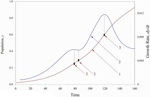
Figure 3. The observations [35] and the model-calculated population with constant parameters: 1 – the sample $\{y_i^{(\delta )}{\}}_{\overline{i=1,11}}$, 2 – the direct problem solution $y{|}_{a_{0,1,2}^{(1)}=const}$, 3 – the inflection area of the sample, 4 – the inflection point of the solution $y{|}_{a_{0,1,2}^{(1)}}$.

The technique of smoothing spline [56] is applied to evaluate the derivatives of a given sample. Based on the smoothness properties of the S-shaped curve under study and the high precision ensured by a spline approximation, the control of the derivatives $dy/dt$ and $d^{2}y/d{t}^2$ is not a complicated condition.

6.1. The identification of the constant parameters

The first step of the simulation is the estimation of the parameters by the given sample $y^{(\delta )}$ for the traditional case $a_{0,1,2}=constant$. The solution to the inverse problem will be obtained by the regularization method using the scheme (5). The reconstruction is accomplished in the framework of the following formulation: (11) $\begin{array}{rl}& a^{(\delta )}=Arg\underset{a>0}{min}\{a_0^2+a_1^2+a_2^2\}\end{array}$(11) (12) $\begin{array}{rl}& \sum _{i=1}^n{\left[y{\left(t_i\right)|}_a-y_i^{\left(\delta \right)}\right]}^2\le \breve{\delta }\end{array}$(12) where $a_0$ is the initial value of the state $(a_0=y_0)$, the function y(t) satisfies Eq. (6) for given $a_{0,1,2}$, and $\breve{\delta }$ denotes the bound of the observation and simulation errors, which determines the consistency corridor [13]. The latter is determined as the minimum value providing the negative residual in condition (12) (for details, see [13]). The stabilizer in (11) is chosen according to relevant recommendations [14].

The solution to the problem (11) – (12) yielded the parameters $a_0^{(1)}$ = 0.021, $a_1^{(1)}=0.03408,$ and $a_2^{(1)}=0.02957$. The residuals ${\rho }_{rms}^{(1)}={\left\{\sum _{i=1}^n{[y{(t_i)|}_{a^{(1)}}-y_i^{(\delta )}]}^2/n\right\}}^{1/\phantom{12}2}$ = 0.01098 and ${\rho }_{max}^{(1)}=\underset{1\le i\le n}{max}|y{(t_i)|}_{a^{(1)}}-y_i^{(\delta )}|$ = 0.0219 were obtained.

The reconstruction demonstrates that the population’s state calculated by the model with constant parameters has one inflection point (Figure 3, item 4), while the observed state of the population has three inflection points (Figure 3, item 3). The differences are not statistical and have a systematic character. Such deviations indicate the crucial simulation errors of the object’s model with the constant parameters.

6.2. The spline approximation of the sample

The second step of the simulation is the approximation of the sample $y^{(\delta )}$ by smoothing spline to determine the necessary derivatives for the improved matching with the observations. The spline has proved to be satisfactory to approximate discrete observations [56]. The results of the application of the smoothing algorithm [57] are shown in Figure 4. The residuals ${\rho }_{max}^{(2)}$ = 0.007 and ${\rho }_{rms}^{(2)}=$ 0.003 were obtained.

Figure 4. Processing of the observations by smoothing spline: 1 – the population, 2 – the growth rate of the population, 3 – the inflection points of the population.

The existence of the non-unique extremes of the first derivative $dy/dt$ confirms that the non-unique inflection points of the observed population are not numerical oscillations or statistical fluctuations. Therefore, the first derivative variations cannot be recognized as approximation errors, and they exhibit the actual pulsatile and oscillation properties of the process in question.

The second step confirms the necessity to expand the representation of the model’s parameters to ensure the best residual between the observations and the model’s results. Consequently, the parameter $a_2=constant$ should be changed to the function $a_2=a_2(t)$.

6.3. A reconstruction of a variable decline parameter

The third step of the simulation is the regularized reconstruction of the pair $\{a_1$ = constant, $a_2(t)\}$ by a given sample $y^{(\delta )}$. The value $a_0$ is fixed and is determined by the sample. The reconstruction is accomplished in the framework using the following regularization: (13) $\begin{array}{rl}& a_2^{(\delta )}=Arg\underset{}{inf}\left\{W_1{\int }_0^T{a}_2^{2}dt+W_2{\int }_0^T{\left(\frac{d{a}_2}{dt}\right)}^{2}dt+W_3{\int }_0^T{\left(\frac{d^2{a}_2}{d{t}^2}\right)}^{2}dt\right\}\end{array}$(13) (14) $\begin{array}{rl}& \sum _{i=1}^n{[{y\left(t_i\right)|}_{a_{1,2}}-y_i^{\left(\delta \right)}]}^2\le {\breve{\delta }}_1\end{array}$(14) (15) $\begin{array}{rl}& {\int }_0^T{\left|\frac{dy}{dt}\right|}_{a_{1,2}}-\frac{d\tilde{y}}{dt}|dt\le {\breve{\delta }}_2\end{array}$(15) (16) $\begin{array}{rl}& {\int }_0^T{\left|\frac{d^{2}y}{d{t}^2}\right|}_{a_{1,2}}-\frac{d^2\tilde{y}}{d{t}^2}|dt\le {\breve{\delta }}_3\end{array}$(16) where T is the final time of the observations and $W_{1,2,3}$ denotes the weight coefficients. The stabilizer in (13) is chosen according to relevant recommendations [58].

The additional consistency conditions (15) and (16) magnify the matching with the sample. The introduction of condition (15) facilitates the elimination of the uncertainty when selecting the node of the second sought function and if the solution is determined on the expansion interval. The two new nodes are identified according to the consistency condition for both the function and its derivative. The magnitudes are determined as the minimum values providing the negative residuals of the consistency conditions.

The solution to the problem (13) – (16), following the identifiability conditions (Section 5), is divided among the sought parameters and built separately for the parameter $a_2$ on the given set of fixed values $a_1$. The interval of the parameter $a_1$variation is expressed by the first step and can be defined as 0.0030 < $a_1^{{}^{\mathrm{\prime }\mathrm{\prime }}}$< 0.0035.

This case concerns the reconstruction of the complicated dependence of the parameter $a_2$ on time, where a large number of nodes N >> n is required for the satisfactory approximation of the sought quantity. All of the transitions from a small node approximation to its vast number will be performed by controlling the solution’s complexity measure as it requires the locally sequential refinement [13].

The desired parameter $a_2$ was approximated by the piecewise linear function (17) $a_2=\frac{{\chi }_{i+1}^{}-{\chi }_i^{}}{{\tau }_{i+1}-{\tau }_i}+\frac{{\tau }_{i+1}{\chi }_i^{}-{\tau }_i{\chi }_{i+1}^{}}{{\tau }_{i+1}-{\tau }_i}t,{\tau }_i\le t\le {\tau }_{i+1},i=\overline{1,N-1}$(17) where $\{{\tau }_i{\}}_{i=\overline{1,N}}$ is the approximation grid, $\mathrm{X}=\{{\chi }_i^{}{\}}_{i=\overline{1,N}}$ denotes the sought nodes of the function $a_2(t)$, and N is the number of nodes.

The solution to the problems (13) – (16) and the locally sequential refinement when the node number N is increased from N = 11 (according to the volume n = 11) to N = 180 yielded the residuals ${\rho }_{max}^{(3)}$ = 0.01203 and ${\rho }_{rms}^{(3)}$ = 0.004469. For the consistency corridors ${\breve{\delta }}_1=0.025,{\breve{\delta }}_2=0.01$, and ${\breve{\delta }}_3=0.001$, the sequential solutions (Section 5) give the parent element $a_1^{(3)}$ = 0.0303596, and the function $a_2^{(3)}$ depicted in curve 1 of Figure 5. The determination of the parent element is represented in Table 2. The stabilizer (13) was used as a minimum shift criterion due to missing information about the behavior of the solution at t → ∞. The observed and model-calculated inflection points fit together well. The calculated functions $y{|}_{a^{(3)}}$ and $dy/dt{|}_{a^{(3)}}$ are virtually the same as the results of the spline approximation of the sample (Figure 4). A good agreement with the sample does not require further specification of the parameter $a_1$ as a function over time.

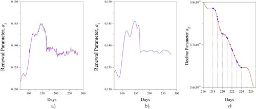
Figure 5. The reconstruction: 1– $a_2^{(3)}$ by the locally sequential refinement, ${\rho }_{rms}^{}{|}_{a_{1,2}^{(3)}}$ = 0.004469; 2– ${\tilde{a}}_2$ by the formula (18),${\rho }_{rms}^{}{|}_{a_1^{(3)},{\tilde{a}}_2}$ = 0.00937; $1/a_1^{(3)}$ = 33.0.

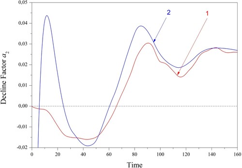
Table 2. The solutions to the inverse problems (13) – (16) for the different α₁ and the allocation of the parent element: item 7 – the minimum of the stabilizer, item 10 – the parent element.

#	$a_1$	Stabilizer (13)	$a_2{|}_{t=0}$	$a_2{|}_{t=160}$	$\mathrm{\Lambda }$	Shooting $a_2{|}_{t=0}$
1	0.03300	0.28686580	0.0161405	0.0285415	0.0024	−0.12009
2	0.03200	0.22001042	0.00105456	0.0274765	0.0014	−0.07463
3	0.03100	0.19202371	0.00009819	0.0271296	0.0004	−0.02918
4	0.03090	0.19035260	0.0000856769	0.0270345	0.0003	−0.02463
5	0.03080	0.18937900	0.0000811075	0.0269352	0.0002	−0.02009
6	0.03070	0.18744988	0.0000705780	0.0268116	0.0001	−0.01554
7	0.03060	0.18635412	0.0000495330	0.0267949	0	−0.01100
8	0.03050	0.18641411	0.0000024956	0.0260564	−0.00001	−0.00645
9	0.03040	0.18928670	0.0000013815	0.0259858	−0.00020	−0.00191
10	0.0303596	0.19071940	−0.0000786108	0.0259731	−0.000241	−0.000072727
11	0.03030	0.19314427	−0.0000854877	0.0257162	−0.0003	0.00263
12	0.03020	0.20192082	−0.000186326	0.0256957	−0.0004	0.00718
13	0.03010	0.20901307	−0.000220475	0.0252427	−0.0005	0.01172
14	0.03000	0.22177508	−0.00692703	0.0249941	−0.0006	0.01627
15	0.02900	0.31305743	−0.02434342	0.0242376	−0.0016	0.06172

The reconstruction by the regularization (13) – (16) expresses the improvement of the growth dynamics simulation. Note that the type of the function $a_2(t)$ identified can be satisfactorily represented by the small node number N only if the sought function’s character is known beforehand. Otherwise, a fine mesh of an approximation is required, causing an increase in the number of the nodes N. The theoretical and practical advantage of the locally sequential refinement is that the reconstruction of the unknown function $a_2(t)$, whose satisfactory approximation requires 180 nodes, uses the sample with 11 measurements.

6.4. Growth features

As it turns out, the parameter $a_2(t)$ has a sinuous character (Figure 5). There are periodic changes in the prevalence between the appearance and disappearance factors. The behavior of the parameter $a_2(t)$ confirms its definition as a decline factor because its increase gives rise to the growth diminution (Figures 4 and 5).

In the case $a_1=constant$, the parameter $a_2$ tends to a non-zero value with the minimal amplitude, which expresses the steady state of the object. In the steady state, the equilibrium occurs between factors that determine the appearance and disappearance of object elements. If the parameter $a_2$ is identified as the constant value, then the residuals ‘observations – model state’ is increased significantly, primarily at the lag stage of the population growth.

Note that the parameter $a_1$, known as the Malthusian parameter and often determined as the growth rate, has the dimension [1/time]. The results demonstrate that it is the frequency of growth renewal (Figure 5), and the value $1/a_1$ determines the time of the renewal. Although the specified time changes during the object’s growth, the value $1/a_1$ gives the average estimate of the time of the increase–decrease cycle. Consequently, it is more correctly say that the parameter $a_1$ determines the frequency of the renewal − declined growth cycle than the growth rate.

6.5. A direct determination of the decline parameter a₂

To validate the estimate of the parameter $a_2(t)$, let us determine the value ${\tilde{a}}_2$ directly from Eq. (6) as follows: (18) ${\tilde{a}}_2=\left(a_1\tilde{y}-\frac{d\tilde{y}}{dt}\right)/{\tilde{y}}^2,$(18) where $\tilde{y}$ and $d\tilde{y}/dt$ denote the spline approximation of the sample and its derivative. The parameter ${\tilde{a}}_2$ is shown in curve 2 of Figure 5 for $a_1^{(1)}$ = 0.03408, which is determined into the framework of the first step.

The comparison of ${\tilde{a}}_2$ with the regularized solution $a_2^{(3)}$ expresses the satisfactory consistency at the large time values and the weak consistency at the initial stage. To determine the simulation errors that occur when the smoothed function ${\tilde{a}}_2$ is used, the solution to the direct problem (6) was obtained for the parameters $a_0^{(4)}$ = $y_1^{(\delta )}$, $a_1^{(4)}$ = $a_1^{(3)}$, and $a_2^{(4)}$ = ${\tilde{a}}_2$. In this case, the residuals were ${\rho }_{max}^{(4)}$ = 0.0156 and ${\rho }_{rms}^{(4)}$ = 0.00937. The latter shows the simulation error growing relative to the third step, ${\rho }_{max}^{(4)}$ <${\rho }_{max}^{(3)}$ and ${\rho }_{rms}^{(4)}<{\rho }_{rms}^{(3)}$. Therefore, the spline approximation alone is not sufficient for the complete object simulation, despite the high accuracy of the sample approximation. The spline approximation can be considered as an initial guess when $a_1=constant$.

Concerning the application of the formula (18), there are some things to note.

First, it includes the parameter $a_1$, which is unknown in the case of the spline approximation of the observations. Here, its value was taken from the first step of the simulation. Second, the invariant transformation (9) shows that a small shift in $a_1$ will lead to significant changes in the parameter ${\text{a}}_2$ at the initial stage of the growth process (Figure 5). Therefore, formula (18) yields a higher deviation between the identified and actual parameters in the initial stage. The locally sequential refinement provides the reconstruction with higher accuracy than the smoothing spline. The appcation of smoothing spline cannot exclude the uncertainties of the parameter $a_1$ determination.

Finally, it should be noted that the above-described technique does not render insignificant the lack of information on measurement errors. Introducing the noise level into the formulation problem remains crucial for improving the estimation accuracy and solution smoothness.

7. Patterns of the COVID-19 spread and progression in a given region

The previous section reveals the critical feature of object growth. As it turns out, the parameter that expresses the difference between the disappearing and appearing elements during the object growth has an oscillatory nature, while another parameter can remain constant. The size of the above-considered sample cannot reveal other features of the growth. In particular, the specification of the parameter $a_1$ as a function of time cannot be executed. A large-size sample is required to identify all the parameters of growth-dependent details, and a more complicated function should be reconstructed to describe the desired quantities more accurately. The latter leads to a high number of approximation nodes. Also, the differences between conditions acting in a natural environment and laboratory settings should be stressed. The reconstruction in the context of the laboratory environment was considered in Section 6. Here, we determine the patterns of the COVID-19 spread into a given region, considering both parameters $a_{1,2}$ as functions of time.

The application of the Verhulst equation with the variable parameters $a_{1,2}(t)$ means that all the factors of disease spread are considered in the framework of the general balance ‘expended − reached’. The mathematical model of this balance facilitates revealing the growth features that cannot be identified applying the models mentioned in Section 4. Especially, the proposed processing reconstructs actual object behavior without any additional information on its features. Postulating the functional properties of the required values is not performed. The observations will be processed under the condition that the reconstruction should ensure the small residual between the sample $y^{(\delta )}$ and the model-calculated state function y.

Consider the total coronavirus cases in Germany from January 27, 2020 (the last day with a single coronavirus case) to April 15, 2021 (day 441) (the source [59]). The sample $\{y_i^{(\delta )}{\}}_{i=\overline{1,n}}$, n = 441 and its spline approximation are shown in Figures 6 and 7. As seen, there are many inflection points because of the periodical changes during seven days, which exhibit the oscillatory nature of growth. The adequate representation of such behaviour cannot be achieved when the simulation is based on the traditional decomposition to the simple processes [60].

Figure 6. The total coronavirus cases in Germany, the source [59]: 1 – the sample $y^{(\delta )}$, 2 – the spline approximation, $\tilde{y}$.

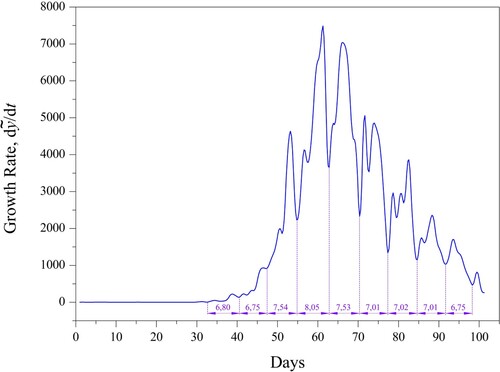
Figure 7. The spline approximation of the growth rate, $d\tilde{y}/dt$, the period of the renewal and decline cycle, $1/a_1$ = 6.98 days.

7.1. The identification of the constant parameters

The first step of the simulation is the estimation $a_{0,1,2}=constant$ by the given sample $y^{(\delta )}$ at the observational time before the second wave appears (n = 130). The solution to the inverse problem was determined by the regularization scheme (11), (12). The reconstruction yielded the parameters $a_0^{(5)}$=20.71, $a_1^{(5)}=0.13275,\text{and }{a}_2^{(5)}={0.804459}_{{10}^{-6}}$. The residuals ${\rho }_{max}^{(5)}=\underset{1\le i\le n}{max}|y{(t_i)|}_{a_{0,1,2}^{(5)}}-y_i^{(\delta )}|$ = 7153.6 and ${\rho }_{rms}^{(5)}=\{\sum _{i=1}^n{[y{(t_i)|}_{a_{0,1,2}^{(5)}}-y_i^{(\delta )}]}^2/{n\phantom{{[y{(t_i)|}_{a_{0,1,2}^{(5)}}-y_i^{(\delta )}]}^2}\}}^{1/\phantom{12}2}$ = 3203.2 were obtained. The large values of residuals show that the model with constant parameters cannot describe the sample adequately. The significant differences between the sample and the model-calculated function occur at the lag stage of the population growth. The initial state $a_0^{(5)}$ is significantly different from its observed value. After this, the initial state is determined by the sample, $a_0=y_1^{(\delta )}$.

7.2. The spline approximation of the sample

The second step of the simulation is the approximation of the sample $y^{(\delta )}$ by the smoothing spline. The residuals between the sample $y^{(\delta )}$ and its spline-approximation $\tilde{y}$ were ${\rho }_{max}^{(6)}$ = 0.37597 and ${\rho }_{rms}^{(6)}=$ 0.0995. The parameter ${\tilde{a}}_2^{(6)}$ determined by the formula (18) with previously reconstructed $a_1^{(5)}$ is shown in Figure 8.

Figure 8. The parameter ${\tilde{a}}_2^{(6)}$ determined by the formula (18): (a) the initial period, (b) the attenuation period .

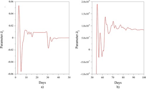
The pulsatile character of the function $d\tilde{y}/dt$, together with the periodic structure repeating during 7–8 days (Figure 7), expresses the existence of the essentially non-heterogenic environment of the object growth. Consequently, it should be explained why the local changes in the growth rate do not constitute a numerical instability but describe a regular property of the process under study. The processing of experimental data should explain the observed growth’s pulsatile character and reflect the periodic alternation over 7–8 days. The spline application is not sufficient to explain these object properties, despite the high accuracy approximation by them.

7.3. The locally sequential refinement of the model parameters

The third step of the simulation is the regularized reconstruction of the pair $\{a_1$ = constant, $a_2(t)\}$ by the total sample $y^{(\delta )}$. The initial state was chosen from the sample, $a_0$ = 1. The parameter $a_2$ was approximated by the piecewise linear function (17). The regularization was accomplished by the scheme (13) – (16) together with the locally sequential refinement of the reconstruction. The number of the sought function nodes N was sequentially increased from N = 10 to N = 906.

The reconstruction demonstrates that the middle part of the S-shaped curve has the worst sensitivity to the sought parameter variations. The expansion of the approximation nodes, especially in the interval from day 27 to day 125, was coupled with a persistent local instability as the spikes in the sought nodes of the function $a_2(t)$. Therefore, the technique to eliminate the spikes was the locally sequential refinement under the minimization of the stabilizer (13), where the residuals of the conditions (14) – (16) had no positive values. For this purpose, the value of the consistency corridors should be greater than the minimum residuals. The stabilizer’s minimization within the given consistency corridors was implemented, starting from the interval of the local expansion of the approximation and ending with the whole observation interval. Finally, the constant parameter $a_1^{(7)}$ = 0.143238 was determined. Note that the value $1/a_1^{(7)}$ = 6.98 expresses the estimate of the renewal period satisfactorily (Figure 7).

The large residuals with the sample, ${\rho }_{max}^{(7)}$ = 454.8 and ${\rho }_{rms}^{(7)}$ = 99.6 were obtained. This means that the pair $\{a_1^{(7)}=constant$, $a_2^{(7)}(t)\}$ cannot provide the sufficient approximation accuracy of the sample $y^{(\delta )}$. By this, both sought quantities should be considered as the functions of time, $\{a_{1,2}(t)\}$. The identifiability conditions were determined in Section 5. Consequently, the regularization was conducted in two separate schemes. The first one is as follows: $\begin{array}{rl}& a_2^{\left(\delta \right)}=Arg\underset{}{inf}\left\{W_1{\int }_0^T{a}_2^{2}dt+W_2{\int }_0^T{\left(\frac{d{a}_2}{dt}\right)}^{2}dt+W_3{\int }_0^T{\left(\frac{d^2{a}_2}{d{t}^2}\right)}^{2}dt\right\},\\ & \sum _{i=1}^n{\left[y{\left(t_i\right)|}_{a_{1,2}}-y_i^{\left(\delta \right)}\right]}^2\le {\breve{\delta }}_1,\\ & {\int }_0^T\left|{\frac{dy}{dt}|}_{a_{1,2}}-\frac{d\tilde{y}}{dt}\right|dt\le {\breve{\delta }}_2,\\ & \frac{dy}{dt}\ge 0,\end{array}$and the second one is as follows: $\begin{array}{rl}& a_1^{\left(\delta \right)}=Arg\underset{a_1>0}{inf}\left\{W_4{\int }_0^T{a}_1^{2}dt+W_5{\int }_0^T{\left(\frac{d{a}_1}{dt}\right)}^{2}dt\right\}\\ & \sum _{i=1}^n{\left[y{\left(t_i\right)|}_{a_{1,2}}-y_i^{\left(\delta \right)}\right]}^2\le {\breve{\delta }}_1,\\ & {\int }_0^T\left|{\frac{dy}{dt}|}_{a_{1,2}}-\frac{d\tilde{y}}{dt}\right|dt\le {\breve{\delta }}_2,\\ & \frac{dy}{dt}\ge 0,\end{array}$where the sole parameter, $a_1$ or $a_2$, is reconstructed with another fixed parameter, $a_2$ or $a_1$. The reconstruction sequence – first a₂  and then a₁ – is the essential requirement determined in Section 5. The piecewise linear functions approximated the sought parameters. The condition of the non-negative value of the growth rate plays an essential role during locally sequential refinement. The consistency with the second derivative is not considered because, as shown later, the behavior of the function $a_2$ requires special smoothing procedures. The lack of agreement with the first derivative leads to a very strong smoothing of the solution. Therefore, this condition is considered the principal one.

The proposed approach effectively constrains the local numerical instability for a sufficiently detailed approximation scheme (Figure 9). The solution with the general regularization but without the locally sequential refinement is shown in Figure 9(a). The local spikes are typical results of reconstructing the variable parameters of the Verhulst equation. Their restrictions on the locally sequential refinement facilitate the necessary solution smoothing (Figure 9(b)). The typical non-uniform approximation scheme applied during the reconstruction is depicted in Figure 9(c). Depending on the complexity of the reconstructed fragment, the solution was sought using 4–10 nodes in each interval between two adjacent observation days.

Figure 9. The parameter reconstruction: (a) the general regularization (5) without the locally sequential refinement, (b) the general regularization (5) together with the locally sequential refinement, (c) the used approximation scheme.

The residuals ${\rho }_{rms}^{(8)}=$ 14.1 and ${\rho }_{max}^{(8)}=$ 62.6 were determined and demonstrate the satisfactory accuracy of the sample approximation. The number of the approximation nodes were $N_{a_1}=$ 578 and $N_{a_2}=$ 1889. For the small extended consistency corridors, ${\breve{\delta }}_1=15.0$ and ${\breve{\delta }}_2={0.65}_{10}^9$, the determined functions $a_{1,2}^{(8)}(t)$ are shown in Figure 10. It reflects the oscillations of the state function y as the regular feature of the process under study (the details are shown enlarged in Figure 10(a)). The consistency with the first and second derivatives of the sample spline approximation was obtained satisfactory (see Supplementary materials).

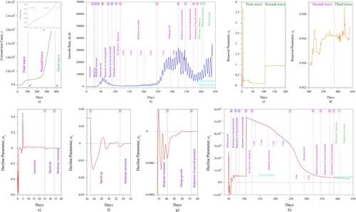
Figure 10. The patterns of the COVID-19 spread in Germany (the symbols $◯1\text{--}◯7$ mark the moments of the dynamics changes).

7.4. Influence of underreporting cases on the estimation

The critical part of the simulation is accounting for the influence of underreporting cases on the solution. For this purpose, the developed approach should demonstrate how the solution structure changes when significant observation errors are taken into account. Also, the obtained functions $a_{1,2}(t)$ contain a lot of local changes. Therefore, it is necessary to explain their meaning, otherwise, they should be considered as local spikes.

The regularized reconstruction is applied, for which the consistency corridors are significantly extended. By this, the stabilizer is minimized as much as possible, and the strong smoothness of the sought functions $a_{1,2}$ is performed.

The consistency corridors were extended up to 20% of the maximum sample value. For this case, the deviations from the current observation were: ±1.4 at the days’ interval (1,27), ±167 at the day’s interval (28,54), ±1261 at the day’s interval (55, 126), ±88.5 at the day’s interval (127, 189), and ±1855 at the day’s interval (190, 440). As seen, the extension of the consistency corridors covers a significant level of underreporting cases, more than 1800 per day. The functions $a_{1,2}^{(9)}$ reconstructed under extended consistency corridors are shown in Figure 11.

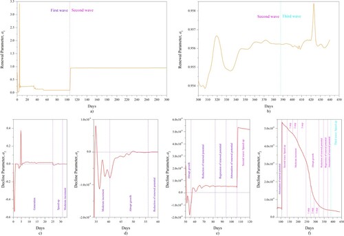
Figure 11. The reconstruction into the large consistency corridor, the worst residuals with observations: ${\rho }_{max}^{}{|}_{i=7}=1.4$, ${\rho }_{max}^{}{|}_{i=49}=167$, ${\rho }_{max}^{}{|}_{i=105}=1261$, ${\rho }_{max}^{}{|}_{i=424}=1855$.

A lot of the local changes in the growth rate were smoothed out. However, even for a high degree of smoothing, a part of the local variations in the function $a_2$ was preserved. This indicates the absence of numerical instability, even at the local level. For the state function $y{|}_{a_{1,2}^{(9)}}$, all the inflection points of the original sample were maintained. The local variations of the growth rate $dy/dt$ that determine the existence of the inflection points, and all the points of the parameters behavior changes were preserved.

The extension of the consistency corridors and the smoothing solution strongly indicates that the functions $a_{1,2}^{(8)}(t)$ and $dy/dt{|}_{a_{1,2}^{(8)}}$ do not have numerical oscillations. Their diversity expresses the non-uniform viral habitat. Note that under laboratory conditions (Section 6), the functions $a_{1,2}^{(3)}(t)$ and $dy/dt{|}_{a_{1,2}^{(3)}}$ did not show the pulsatile characters found in the coronavirus cases (compare Figures 5 and 10).

Although strong smoothing ensures the stable identification of growth trends, simplifying the solution to smooth the desired functions maximally means that the corresponding reconstruction excludes several essential factors of the system ‘virus–environment’ that are important for practical diagnostic purposes. Nevertheless, the reconstruction with the minimum allowable consistency corridors expresses the actual growth dynamics with more details.

Thus, the regularization scheme (5) facilitates the solution smoothing into the allowable consistency corridors and ensures the conservation of the main functional properties of the solution, including the periodic alternation over 7–8 days (Figure 11(f)).

7.5. The nature of the Verhulst equation parameters

The processing of the experimental data of the coronavirus cases demonstrates the existence of the following general features of growth.

The parameter $a_1$, which was early defined as a renewal factor of growth, can be considered as the estimate of renewal frequency. The constant value $1/a_1^{(7)}$ approximately determines the time between the maximum number of disappearance elements and the maximum number of appearance elements (Figure 7). Generally, its behavior after the initial stage can be defined as a piecewise constant function. At the initial stage, the renewal parameter has a completely pulsatile character. If the environmental conditions are not aimed at reducing growth, the parameter $a_1$ appears to be a weakly varying function (see Section 6).

The reconstruction of the parameter $a_2$ confirms its oscillatory nature. It integrally expresses the factors that decline object growth. The parameter $a_2$ takes both negative and positive values. Negative values mean that the number of newborns dominates over the number of deceased individuals. The most active phase of the growth occurs when the appearance elements of the object dominate over the disappearance elements. The phases of generation and speed-up of growth are characterized by the presence of an extensive zone with negative $a_2$. On the contrary, positive values represent the domination of deceased individuals over newborns. Its higher value gives rise to a decreasing growth rate and a population gain. The appearance of a jump of the parameter $a_2$ (Figures 10(f) and 11(f)) can reflect the essential object modification and its transformation to a new structure.

7.6. Phases of the COVID-19 progression in a region

The results obtained depict the specific features of the COVID-19 spread in a region. Figure 10 demonstrates that the COVID-19 progression is divided into seven phases. The phase of viral activity is defined as an area where the function $a_2$ has the typical behavior that differs from other areas. Each of the phases has its own substructure, which expresses a difference in the tendency to grow. The following key points determine these phases.

The first point, marked by the symbol $◯1$, expresses the end of the population generation. A characteristic feature of the corresponding phase is the existence of the highest renewal potentials. A vast area with negative values shows the initial renewal potential of the emerging population. This area corresponds to the most significant changes in the parameters $a_{1,2}$. After this point, a transition occurs with constant and moderate increments, starting from the slow rate to the growth mode (Figure 10(f)). The corresponding first phase can be determined as a generation of population.

The second point, marked by the symbol $◯2$, reflects the end of the small growth rate $dy/dt$. The changes in the decline parameter behavior at the interval $◯1\text{--}◯2$ can be seen in Figure 10(f). In this zone, the oscillation of the amplitude of the decline parameter $a_2$ is decreasing, having mainly negative values. The changes in the domination between the appearance–disappearance factors have considerable amplitude and frequency. Here, the distinctive feature is a sequential decrease in the amplitude of oscillations to a specific value, weakly changing during the next phase. The second phase can be determined as the speed-up of growth.

The third point, marked by the symbol $◯3$, indicates the transition to the exponential stage after the moderate increments of growth. Figure 10 (g) reflects that at the interval $◯2\text{--}◯3$ a distinctive feature is the slowly changing amplitude of oscillations around a certain value. Here, the appearance factor continues its dominance for the object renewal. The region between the second and third points is the most unstable in a numerical sense. Consequently, the latter generates the reconstruction instabilities. The relevant phase can be determined as a moderate increment of growth.

The fourth point, marked by the symbol $◯4$, determines the achievement of the maximum growth rate (Figures 10 (g) and (h)). A characteristic feature of this phase is the contraction of the oscillations of the decline parameter to the vicinity of the zero value. It is indicative that in this area, the parameter $a_2$ diminishes alongside the transition from negative to positive values. The relevant phase at the interval $◯3\text{--}◯4$ can be determined as abrupt growth.

The fifth point, marked by the symbol $◯5$, denotes the right boundary of the zone, in which the difference between the growth factors starts to minimize near a specific small positive value (Figure 10 (h)). The amplitude of the decline parameter $a_2$ is large. The relevant phase at the interval $◯4\text{--}◯5$ can be defined as a reduction of renewal potential.

The sixth point, marked by the symbol $◯6$, express the moment when the variability of the decline factor $a_2$ is systematically reduced (Figure 10 (h)). The stable decline of the object’s renewal occurs, and the oscillations tend to have a smaller amplitude. The relevant phase at the interval $◯5\text{--}◯6$ can be determined as a regression of renewal potential.

The seventh point, marked by the symbol $◯7$, expresses the end of the zone in which the variability of the decline parameter is tiny, and its value tends to be constant (Figure 10 (h)). Zeroing the renewal potential means complete termination of the renewal and transition to the stable equilibrium ‘object–habitat’. The latter is associated with a plateau in the S-shaped curve. The relevant phase at the interval $◯6\text{--}◯7$ can be determined as attenuation of renewal potential.

Further consistent reduction of the amplitude of the decline factor is not a prerequisite in the general case. Previously, it was determined that a cyclic repetition of a virus outbreak without introducing its pathogen from outside is the result of a phase change of populations [61]. The cyclic oscillations in the parasitic system were mathematically proved [62] and analyzed [63]. In this regard, the use of Eq. (6) is valuable in assessing the potential for further population growth. The difference between the curve and the asymptote line (the green lines in Figure 10 (h)) expresses the appearance of the new wave of the virus progression.

The reconstruction of the decline parameter behavior in the attenuation phase is critical. If the decline parameter does not tend to the constant and decreases, then the viral population tends to a new spread wave. The decrease in the decline parameter at the end of the curve (Figure 10 (h)) expresses the third wave occurrence.

It should also be noted that the reconstruction expresses a wide range of oscillation features of the growth process. They include large and very small amplitudes, relaxation with fast phase changes, slow, moderate, and quick frequencies [64], complexity and self-organization [65]. Furthermore, all these features appear within the framework of the individual process.

Thus, the parameters $a_{1,2}$ can reflect real virus dynamics, although they represent the phenomenological properties of the object in a generalized form. The described seven phases express the life cycle of the COVID-19 progression.

7.7. Renewal potential

The existence of the different phases of the object growth demonstrates the necessity to introduce the notation that defines the virus’ activity from the viewpoint of its progression. Figure 10 exhibits the difference between the maximum and minimum values of the parameter $a_2$ within one phase of the life cycle. The high value of this difference reflects the great potential of the object renewal, and a low value represents a low potential in this case. Consequently, this difference is proposed to define as the renewal potential. Note that the introduced renewal potential is correlated with the notation of population strength [66].

The behavior of the renewal potential expresses the essential characteristic of the object evolution: if its value increases, then the virus spread rises. The trend of the decline parameter $a_2$ toward negative values is indicative of the spread dynamics. Such behavior expresses that newborn individuals prevail over the number of dying individuals.

Keep in mind that the parameter $a_2$ covers a wide range of values, from large to very small. Therefore, changes in the renewal potential should only be seen in connection with the current spread phase and not compared with its absolute maximum. The local behavior of the renewal potential determines the phase fading or the continuation of spread.

7.8. Environment change

Let us consider the existence of the features described above when the environment of the COVID-19 spread is changed. Three countries were selected, which have quite different dynamics of the COVID-19 spread. The coronavirus cases for Sweden, Switzerland and Brazil [59] were processed.

For the case of Sweden, the sample was $\{y_i^{(\delta )}{\}}_{i=\overline{1,370}}$, and the number of sought nodes of the linear piecewise approximation (17) was $N_{a_1}=$ 444, $N_{a_2}=$ 2200. The obtained residuals, ${\rho }_{rms}^{(10)}=$ 1.1 and ${\rho }_{max}^{(10)}=$ 12.9, are small and demonstrate the satisfactory approximation of the sample and satisfactory discretization in the parameters sought. For the case of Switzerland, the sample was $\{y_i^{(\delta )}{\}}_{i=\overline{1,205}}$, the number of sought nodes was $N_{a_1}=$ 548, $N_{a_2}=$ 941 and the residuals ${\rho }_{rms}^{(11)}=$ 1.7 and ${\rho }_{max}^{(11)}=$ 15.9 were obtained. For the case of Brazil, the sample was $\{y_i^{(\delta )}{\}}_{i=\overline{1,350}}$ and the number of sought nodes was $N_{a_1}=$ 2151, $N_{a_2}=$ 2139. The obtained residuals, ${\rho }_{rms}^{(12)}=$ 352.86 and ${\rho }_{max}^{(12)}=$ 2255.6, despite a large number of nodes $N_{a_{1,2}}$, are in order higher than those in other cases. Comparing the obtained results in all four cases, we can observe that a significant level of residuals for the case of Brazil recommends paying attention to the errors in the reported sample.

The reconstruction by the locally sequential refinement approach demonstrates that the COVID-19 behavior in different countries is similar to the one described in subsection 7.5. Each of the considered options reflects all seven phases of the viral activity. At the same time, each of them has its traits and features, found in the details of any phase of the activity.

For example, for Sweden (Figure 12(a)), the prolonged phase of abrupt growth is special. Here, due to the appearance of various modifications of the decline parameter $a_2$ (five steps), the renewal potential was maintained at a high level for a considerable period. The short intervals of the generation and speed-up phases are specific to Switzerland (Figure 12(b)). Also, a rapid exit to a stable state of the first wave has taken place. For Brazil (Figure 12(c)), the beginning of the generation phase occurs in a positive parameter domain. Also, the existence of a non-regular behavior of the decline parameter $a_2$ attracts the attention in the case of Brazil. Notably, the decline parameter for the cases of Switzerland and Brazil tends to zero from below, in contrast to the cases of Germany and Sweden, where the decline parameter tends to zero from above. The parameter a₁  has the corresponding behaviour, and for the case a₂→-0 the character of the parameter a₁ is similar to the delta-function, Figures 12(b) and 12(c). Physically, this means that there is no need for constant additional energy to continue the growth. It is required sporadically. If the reconstruction of all the above cases are performed with the assumption that a₁ = constant, then the asymptotic of the parameter a₂ is similar to the case described in Section 6. Such a simulation gives rise to very significant residuals. Nonetheless, all determined seven phases of the life cycle were retained despite the substantial simplification. The repeatability of the structure of the function a₂(t), including the strong simplification a₁ = constant , indicates the stability of the character of the COVID-19 life cycle during the simulation.

Figure 12. The parameters reconstruction for the different countries, the source of the COVID-19 cases [59]: (a) Sweden; (b) Switzerland; (c) Brazil.

The results obtained (Figures 10 and 12) demonstrate that in the sense of the balance ‘expended–reached’, the second wave of the disease progresses similar to its first wave. Also, the reconstruction expresses the appearance of the third wave following the factor of the decline parameter decrease. The decline parameter shows similar characteristics in different countries.

The description of other features of the virus spread requires the investigation of new cases of the COVID-19 spread. Undoubtedly, the features identified above should be confirmed by more abundant datasets in different regions in a future study. The present investigation is limited to demonstrate the possibility of obtaining valuable information on the virus spread using the Verhulst equation that can establish the current activity phase of the life cycle and reflect its spread potential.

An essential feature of the used observations and the corresponding processing is considering the large geographical areas with different regions. Such heterogeneity certainly averages the final result. However, the application of the proposed approach separately for any part of the general area – state, region, district or city – will make it possible to promptly differentiate the virus activity levels and localize the most dangerous areas. Undoubtedly, further development of this approach requires considering spatial factors and the transition to parabolic models.

Summarize the results of Section 7. The above-described phases mean the specification of the commonly known growth stages – lag, exponential, stable – by the additional phases of the virus activity and its progression. The processing of the experimental data reflects that the COVID-19 life cycle includes seven phases: population generation, speed-up of growth, a moderate increment of growth, abrupt growth, reduction, regression, and attenuation of renewal potential. All the listed points are criteria for phase emergence. The introduced seven points facilitate the monitoring of disease outbreaks and can specify its next progression. The information is valuable for preclinical control of a virus spread in a region. All numerical details of the reconstruction and simulation are represented in the supplementary materials.

8. Discussion

The results show the absence of constant properties of growth. From traditional notions of the growth dynamics, the reconstructed parameters can be recognized as artificial functions. As such, the consequences require justification at the theoretical and applied levels.

From a simulation theory, the sense and interpretation of the parameters $a_{1,2}$ were described in [25,26]. Based on this, the variations of the Verhulst equation’s parameters have a clear explanation. However, the reconstruction of these parameters has ill-posed problem attributes: the violation of one-to-one correspondence, numerical oscillations, and weak sensitivity to the parameter variation are typical to the identification of Eq. (6). The following theoretical decisions were implemented to take into account these features of the problem formulation.

The inverse problem formulation with variable parameters is characterized as a role by the invariant properties regarding desired quantities. The proposed determination of a parent element of invariant families expresses the principle of an identifiability justification when sought parameters belong to an invariant family. It consists of constructing a sequence of the solutions on the invariant elements and allocating a parent element based on different reconstructions.

The essential part of the reconstruction is adequately accounting for the multiple characters of samples and matching the solution with the noise level separately for each element of the observation set. The proposed regularization under separate observation matching facilitates the stable estimation, adequate reconciliation with samples, and reconstruction into the consistency corridor framework with the given observations. The introduced stabilizers have successfully restricted the desired solution throughout the domain space and local region. The estimation of complicated functions without locally sequential refinement has given rise to arbitrary solutions. The local spikes were successfully restricted with the stabilizer minimization into the consistency corridors of each matching condition.

The locally sequential refinement facilitated the solution stabilization and performed the stable detailing of the restored functions. It turned out to be possible to identify the sinuous function, the approximation basis N of which was an order of magnitude larger than the volume n of the given sample, N >> n. The stable extension of the approximation basis provided revealing significant information regarding the features of the growth.

The obtained solutions express the sample’s requirements that should ensure the best estimation of the growth parameters. The observations at the initial and final stages of growth are critical. The observations in the middle part of the S-shaped curve allow for significant variations of the sought parameters. The final structure of the best sample can be guided in the framework of the experimental design.

A comparison of the cases studied − the experiment in laboratory conditions (Section 6) and the observations in the virus’ habitat (Section 7) − demonstrate the critical influence of the environment on population growth. For the non-laboratory conditions, the existence of a non-uniform habitat of the virus is typical. Sufficient detailing of the reconstructed properties was performed only over the large-size basis of the sought parameter approximation.

The parameter oscillations’ character reflects a strictly defined structure for different virus habitats. This structure is correlated with the observed growth rate oscillations. The structure repeatability for the different spread dynamics and simulation cases indicates that the decomposition into the proposed seven phases is adequate. Undoubtedly, the generalization of this conclusion requires further investigation of other biological objects.

The maintenance of such feathers as the spread’s dynamics, trends of population growth, its contraction, and the nature of the spread phases during the extension of the consistency corridors up to 20% (see subsection 7.4) are confirmed by the maintenance of the functional properties mentioned above for cases of sample revisions. For example, the observations of the coronavirus cases in Sweden [59] were revised more than once. Each change was up to 5% of the current value. The final revision differed from the initial data up to 15%, leading to significant discrepancies between the observations and the model state. Correspondingly, the parameters $a_{1,2}$ were identified anew. The renewal estimates retained their previous nature of the spreading phase (Figure 12(a)). So, the nature of the obtained solution turns out to be resistant to the extensive local sample variations. At the same time, the reconstruction can demonstrate the unsatisfactory local consistencies in the areas with gross systematic errors in observations (the areas of the irregular behavior of the parameter $a_2$, Figure 12(c)).

From the mathematical viewpoint, the significance of the described processing is that the approach based on an approximation of a given discrete set by a function coincided with the phenomenological model. The interpretation of the experimental data applied directly to the explicit parameters of the adequate model without introducing assumed functional properties. The approximant of the sought quantities was not chosen as a function of a predefined behavior. Its functional character was determined by the condition of satisfying the relevant phenomenological law. The adequate object model governs observation fitting. The character of the approximant was reconstructed according to the stable and best sample approximation. The reconstruction does not require introducing the type of the approximant but requires a large number of approximation nodes. The reconstruction method accounts for the numerical features of the ill-posed formulation. Therefore, the obtained solution exhibits the object properties directly from experimental data processing without a postulation of the nature of sought quantities and further estimation postprocessing. The analogues of such representations are MRT and CT diagnostics.

Though the model used here is the simplest simulation of viral dynamics, it determines the basic phenomenological features of object growth in the sense of the balance ‘expended – reached’. In general, the growth properties have very complicated species because the non-heterogenic habitat causes a sophisticated adaptation of the object in question to the environment. Both parameters of the Verhulst equation must be the functions over time to simulate an object’s growth more accurately.

From the biological viewpoint, the obtained results demonstrate that the Verhulst equation reflects the oscillatory paradigm of biological objects [67]. The oscillation nature of the Verhulst equation’s parameters expresses the fundamental feature of chemical kinetics [68,69]. The mechanisms, models, and phenomena causing oscillations in biological and chemical systems are described in many studies [70–76]. Nowadays, the review of the most typical oscillation phenomena in biological systems is proposed [77]. The dynamics of disease spread generally correspond to the homeodynamics paradigm [78].

The reconstructed oscillations (Figures 5, 10, and 12) have analogues in physical chemistry [65,79], biochemistry [80–82], and epidemiology [83,84]. The principle of biological oscillations has mathematically been described before [66]. The reconstructions confirm the opposition principle [66]. In addition to the proposed differential equation governing population dynamics [66], the Verhulst equation expresses an object’s growth when, generally, an object’s kinetic energy is transformed into its potential energy [52]. The renewal potential can be introduced to reflect the spread dynamics. Together with the favorability function [66], they cover general aspects of the interaction of the complex system ‘object–environment’.

The reduction of the SIR model to the Verhulst equation [51] enhances the generalized nature of the Verhulst equation. The reduction means that the Verhulst equation is not a particular case of the simplest processes of the object change but is related and reflects the fundamental features of its growth [85]. The systematic changes of the S-shaped curve convexity–concavity are essentially oscillations that lead to non-unique inflection points (Figure 10). The processing of experimental data demonstrates that the slowly oscillated growth process is characterized by the high-amplitude oscillations of growth rate and intensely varied object adaptation.

Smoothing of most inflection points leads to the loss of essential information about the phenomena in question. The superposition of the growth process by the sum of partial solutions to the Verhulst equation with constant parameters, which starting from the study [60] is very popular in mathematical biology, cannot provide the complete representation of the object behavior.

From the epidemiology viewpoint, the application of the Verhulst equation has shown that it gives an accurate representation of the actual state of the disease progression in a given region. The results reflect the peculiarities of the disease spread in a region of any level (e.g. a district, a city, a region, a country), the tendency of the disease to spread, and the effectiveness of antiviral measures after the COVID-19 outbreak. The application of the Verhulst equation does not exclude the use of other models and supplements the results received through them. Information obtained by the Verhulst equation, despite its non-medical nature, is of paramount practical importance for monitoring and controlling a current situation with the disease spread in a region.

Comparing the outcomes obtained with the SIR-like model to the COVID-19 spread in Brazil [86], several advantages of the Verhulst equation are shown here. First of all, note that the solutions found in [86] do not explicitly reflect the features of the observed state function. For example, the results do not express the existent and observed periodic changes in the state function y and the pulsatile nature of the infected number accession (the function dy/dt). Moreover, the impossibility of interpreting the reconstructed parameters’ behavior in terms of corresponding changes in the observed state function is noted by the authors [86]. In this context, the point of reducing the rate of deaths was not explained [86] while the number of infections increased significantly. It is also unclear, based on the results [86], what properties of the three sought functions reflect the second and third waves of the disease. The Verhulst equation facilitates obtaining comprehensive answers to all of the above questions that resulted from the use of the SIR-like model.

Further investigations as generalized nature of the Verhulst equation and the equation governing population dynamics [66], as well as properties of growth oscillatory behavior can determine new features of biological objects’ dynamics [82]. A deeper understanding of the disease progression requires identifying the mechanisms for the different phases and, based on this, recommendations for controlling the COVID-19 spread in a given region.

9. Conclusions

The main results of the investigation are as follows.

The principle of the allocation of the unique element from invariant families was proposed. Uncertainties caused by the violation of the one-to-one correspondence between a state function and parameters of the Verhulst equation were excluded.

The regularization under the separate matching scheme without the regularization parameter ensured the stable reconstruction within a considerable expansion of the solution’s domain. The proposed scheme can implicate any qualitative and quantitative information. The control of the positive values of the state function and its derivatives were included in the reconstruction procedure. The additional constraints improved the matching with observations.

The essential part of the desired functions specification was the introduction of the additional solution regularization. The locally sequential refinement provided sufficient restrictions of local disturbances when the number of approximation nodes of the sought quantities was significantly higher than the sample size. The general regularization and additional consistency conditions cannot exclude local spikes when the number of approximation nodes is extended. The necessary regularization was performed locally on the interval approximation by the stabilizer minimization within the consistency corridor. The proposed approach demonstrates that large-scale numerical instabilities can be filtered out when small oscillatory functions are reconstructed.

The study purpose – the approach development to reconstruct the extended number of unknowns under a limited volume of initial information – was realised for the classical problem of object growth. The application of the developed approach highlighted novel features of the growth process. The results refine and emphasize the significance of the Verhulst equation as the generalized model of object growth. The variable parameters of the Verhulst equation express the fundamental regularities of the system ‘object − environment’. The behavior of the reconstructed parameters is clearly interpretable and sufficiently informative to reflect the features of the process dynamics. They reveal the detailed characteristics of the object’s interactions and its adaptation to the environment, including the different types of oscillations when the object is changed. The life cycle of the COVID-19 progression was revealed. Finally, the general solution to the Verhulst equation with variable parameters was determined and the invariant of the Verhulst equation was obtained.

Further applications of the developed approach will be directed to the reconstruction of the growth parameters of a broad class of biological objects.

Nomenclature

a	=	desired parameter
$\overline{a}$	=	actual parameter
$\tilde{a}$	=	direct estimation
$\check{a}$	=	element with the minimum measure of the shift
$a_{0,1,2}$	=	parameters of the Verhulst equation
$a^{(\delta )}$	=	reconstructed parameters matched with observation errors
m	=	number of samples
n	=	sample volume
p	=	number of parameters
t	=	time
x	=	spatial coordinate
y	=	state function
$\overline{y}$	=	actual state
$y^{(\delta )}$	=	sample
$\tilde{y}$	=	spline approximation
$\text{Å}$	=	parent element of invariant family
$\mathcal{M}$	=	measure of the second parameter shift
$N$	=	number of approximation nodes
$\mathrm{\wp }$	=	shift of parameters with minimum measure
δ	=	upper bound of noise consistency corridor
$\epsilon$	=	noise
$\eta$	=	shift of the second parameter of invariant family
$\lambda$	=	shift of the first parameter of invariant family
${\rho }_{max}$	=	the absolute residual between observations and model state
${\rho }_{rms}$	=	root-mean-square residual between observations and model state
$\tau$	=	grid of desired function approximation
$\chi$	=	approximation nodes
$\mathrm{\Omega }$	=	stabilizer

Acknowledgements

The author would like to thank the reviewers, whose questions and comments have improved the presentation of the results and have supported the publication.

Disclosure statement

No potential conflict of interest was reported by the author(s).

References

- Mason JC, Handscomb DC. Chebyshev polynomials. Boca Raton: Chapman & Hall/CRC; 2003.
- Tikhonov AN. On determining electrical characteristics of the deep layers of the earth’s crust. Doklady AN USSR. 1950;73(2):295–297.
- Cagniard L. Basic theory of the magneto-telluric method of geophysical prospecting. Geophysics. 1953;18(3):605–635.
- Fisher RA. The design of experiment. Edinburg: Oliver and Boyd; 1937.
- Mulaik SA. Foundations of factor analysis. Boca Raton: Chapman and Hall/CRC; 2009.
- Foucart S, Rauhut H. A mathematical introduction to compressive sensing. New York: Springer-Birhauser; 2013.
- Tikhonov AN, Arsenin V. Solutions of ill-posed problems. New York: Halsted Press; 1977.
- Morozov VA. Methods for solving incorrectly posed problems. New York: Springer; 1984.
- Ivanov VK. On Ill-posed problems. Matem. Sbornik. 1963;61(2):211–223.
- Bakyshinsky A, Goncharsky A. Ill-posed problems: theory and applications. Dordrecht: Kluwer Academic Publisher; 1994.
- Engl HW, Hanke M, Neubauer A. Regularization of inverse problems. Dordrecht: Kluwer Academic Publisher; 1996.
- Gilyazov SF, Gol’dman NL. Regularization of ill-posed problems by iteration methods. Dordrecht: Springer; 2000.
- Romanovski MR. A reconstruction of object properties with significant uncertainties. Inverse Probl. Sci. Eng. 2021;29(3): 318-364. doi:https://doi.org/10.1080/17415977.2020.1782900.
- Romanovskii MR. Regularization of inverse problem. High Temp. 1980;18(1):135–140.
- Shawe-Taylor J, Cristianini N. Kernel methods for pattern analysis. University Press: Cambridge; 2004.
- Alpaydin E. Introduction to machine learning. Cambridge: The MIT Press; 2004.
- Ahuja RK, Magnanti TL, Orlin JB. Network flow: theory, algorithms and applications. New Jersey: Prentice Hall; 1993.
- Weber G-W, Tezel A, Taylan P, et al. Mathematical contributions to dynamics and optimization of gene environment networks. Optimization. 2016;6(2):183–219.
- Breiman L, Friedman JH, Olshen R, et al. Classification and regression trees. Boca Rotan: Taylor & Francis; 1984.
- Friedman JH. Multivariate adaptive regression splines. Ann. Stat. 1991;19(1):1–141.
- Donoho DL, Stark PB. Uncertainty principles and signal recovery. SIAM J. Appl. Math. 1989;49(3):906–931.
- Özmen A, Kropat E, Weber G-W. Robust optimization in spline regression models for multi-model regulatory networks under polyhedral uncertainty. Optimization. 2017;66(12):2135–55.
- Taylan P, Weber G-W, Liu L, et al. On the foundations of parameter estimation for generalized partial linear models with B-splines and continuous optimization. comp. Math. Appl. 2010;60:134–143.
- Özmen A, Weber G-W, Batmaz I, et al. RCMARS: robustification of CMARS with different scenarios under polyhedral uncertainty set. Commun Nonlinear Sci Numer Simulat. 2011;16:4780–7.
- Verhulst PF. Notice sur la loi que la population suit dans son accroissement. Correspondance Mathématique et Physique. 1838;10:113–117.
- Lotka AJ. Elements of physical biology. Baltimore: Williams & Wilkins Co; 1925.
- Pearl R. The biology of population growth. New York: Alfred A. Knopf; 1925.
- Gause GF. The struggle for existence. Baltimore: The Williams & Wilkins Co; 1934.
- Kostitzin VA. Mathematical biology. London: G. G. Harrap & Co; 1939.
- Hutchinson CE. An introduction to population ecology. New Haven and London: Yale University Press; 1978.
- Segel LA. Modeling dynamic phenomena in molecular and cell biology. London: Cambridge University Press; 1984.
- Murray JD. Mathematical biology: I. An introduction. 3rd ed. Berlin Heidelberg: Springer-Verlag; 2002.
- Pastor J. Mathematical ecology of populations and ecosystems. New York: Wiley-Blackwell; 2008.
- Kuttler C. Mathematical models in biology. Munchen: Technische Universitat Munchen; 2009.
- Cornette JL, Ackerman RA. Calculus for the life sciences. A modeling approach. New York: MAA Press; 2015.
- Torrealba-Rodrigueza O, Conde-Gutiérrezb RA, Hernández-Javierc AL. Modeling and prediction of COVID-19 in Mexico applying mathematical and computational models. Chaos, Solitons and Fractals. 2020;138:1–28.
- Zhou X, Ma X, Hong N, et al. Forecasting the worldwide spread of COVID-19 based on logistic model and SEIR model. medRxiv. 2020:1–14. DOI: https://doi.org/10.1101/2020.03.26.20044289.
- Hermanowicz SW. Forecasting the Wuhan coronavirus (2019-nCoV) epidemics using a simple (simplistic) model. medRxiv. 2020:1–10. DOI:https://doi.org/10.1101/2020.02.04.20020461.
- Afonso S, Azevedo J, Gomes da Silva MP. Epidemic analysis of COVID-19 in Brazil by a generalized SEIR model. arXiv. 2020:1–12.
- Wu K, Darcet D, Wang Q, et al. Generalized logistic growth modeling of the COVID-19 outbreak in 29 provinces in China and in the rest of the world. arXiv. 2020:1–34.
- Gopal R, Chandrasekar VK, Lakshmanan M. Dynamical modelling and analysis of COVID-19 in India. arXiv. 2020;arXiv:2005:1–20.
- Fanelli D, Piazza F. Analysis and forecast of COVID-19 spreading in China, Italy and France. Chaos, Solitons and Fractals. 2020;134:1–5.
- Mandal M, Jana S, Nandi SK, et al. A model based study on the dynamics of COVID-19: prediction and control. Chaos, Solitons and Fractals. 2020;136:1–12.
- Nowak MA, Bangham CRM. Population dynamics of immune responses to parameters that influence persistent viruses. Science. 1996;272(5):74–79.
- Chen TM, Rui J, Wang QP, et al. A mathematical model for simulating the phase-based transmissibility of a novel coronavirus. Infect Dis Poverty. 2020;9:1–8.
- Lin Q, Zhao S, Gao D, et al. A conceptual model for the coronavirus disease 2019 (COVID-19) outbreak in Wuhan, China with Individual Reaction and Governmental Action. Int J Infectious Diseases. 2020;93:211–216.
- Morozov VA, Gol’dman NL, Samarin MK. Descriptive regularization method and quality of approximate solutions. J Eng Phys. 1977;33(6):1117–1124.
- Hethcote HW. The mathematics of infectious diseases. SIAM Rev. 2000;42(4):599–653.
- Fitzgibbon WE, Langlaisb M, Morgan JJ. A mathematical model for indirectly transmitted diseases. Math. Biosci. 2007;206:233–248.
- Coronel A, Friz L, Hess I, et al. On the existence and uniqueness of an inverse problem in epidemiology. arXiv:1811.02892v1. 2018:1-12.;DOI:https://doi.org/10.1080/00036811.2019.1608964.
- Kermack WO, McKendrick AG. A contribution to the mathematical theory of epidemics. Proc. R. Soc. Lond. A. 1927;115:700–721.
- Leitmann GA. Minimum principle for a population equation. J Optim Theory Appl. 1972;9(2):155–156.
- Huang NE, Qiao F, Wang Q, et al. Herd immunity vs suppressed equilibrium in COVID-19 pandemic: different goals require different models for tracking. medRxiv. 2020:1–39. DOI:https://doi.org/10.1101/2020.03.28.20046177
- Romanovski M. Upper bound of experiment informativeness. Inverse Problems Eng. 2003;11(5):375–389.
- Romanovski M. Heat experiment design: factors of identification error reduction. Inverse Problems in Sci and Eng.2006;14(2):129–156.
- Wahba G. Spline models for observational data. Philadelphia: SIAM; 1990.
- Reinsch CH. Smoothing by spline functions. Numer Math. 1967;10:177–183.
- Romanovskii MR. Regularization of inverse problems by the scheme of partial matching with elements of a set of observations. J Eng Phys. 1982;42(1):92–98.
- Worldometer. Available from https://www.worldometers.info/coronavirus/#countries.
- Pearl R. The curve of population growth. Proc. American Philos. Soc. 1924;63(1):10–17.
- Belyakov VD, Golubev DB, Kaminsky GD, et al. Self-regulation of parasitic systems. Moscow: Meditsina; 1987; (in Russian).
- Kolesin ID. Cyclical fluctuations in the epidemic process model. J Dif. Eq. 1996;32(9):1289–1290.
- Rozhnova G, Nunes A. Fluctuations and oscillations in a simple epidemic model. Physical Review E. 2009;79:1–5.
- Bainov DD, Mishev DP. Oscillation theory of operator-differential equations. Singapore: World Scientific; 1995.
- Mikhailov AS, Ertl G. Chemical complexity. self-organization processes in molecular systems. Switzerland: Springer International Publishing; 2017.
- Chester M. A fundamental principle governing populations. Acta Biotheor. 2012;60:289–302.
- Murray JD. Lectures on nonlinear differential equation models in biology. Oxford: Clarendon Press; 1977.
- Lotka AJ. Contribution to the theory of periodic reactions. J Phys. Chem. 1909;14:271–274.
- Bray W. A periodic reaction in homogeneous solution and its relation to catalysis. J Amer Chem Soc. 1921;43:1262–1267.
- Frank-Kamenetskii DA, Salnikov IE. About the possibility of self-oscillations in a homogeneous chemical system under quadratic autocatalysis. Zh Fiz Khim. 1943;17(1):79–86. (in Russian).
- Frank GM. Oscillatory processes in biological and chemical systems. Moscow: Nauka; 1967; (in Russian).
- Chance B, Ghosh AK, Pye EK, et al. Biological and biochemical oscillators. New York: Academic Press; 1973.
- YuM R, Stepanova NV. Chernavsky DS. mathematical modelling in biophysics. Moscow: Nauka; 1975; in Russian.
- Goldbeter A. Biochemical oscillations and cellular rhythms: the molecular bases of periodic and chaotic behaviour. Cambridge: Cambridge university press; 1996.
- Maroto M, Monk NAM. Cellular oscillatory mechanisms. New York: Springer; 2009.
- Rubin A, Riznichenko G. Mathematical biophysics. New York: Springer; 2014.
- Janson NB. Nonlinear dynamics of biological systems. Contemporary Phys. 2012;53(2):137–168.
- Walleczek J. Changing paradigms in biomedicine: implications for future research and clinical applications. self-organized biological dynamics and nonlinear control. c: Cambridge University Press; 2000. 409–420.
- Gurel D, Gurel O. Oscillations in chemical reactions. Berlin: Springer; 1983.
- Zeuthen E. Growth as related to the cell cycle in single-cell cultures of tetrahymena piriformis. J Embryol Exp Morph. 1953;1(3):239–249.
- Ghosh A, Chance B. Oscillations of glycolytic in intermediates in yeast cells. Biochem. Biophys. Research Comm. 1964;16(2):174–181.
- Yang LZ, Yang M. Modeling biological oscillations: integration of short reaction pauses into a stationary model of a negative feedback loop generates sustained long oscillations. J Comp. Bio. 2019;26(10):1050–1066.
- Rozhnova G, Nunes A. SIRS dynamics on random networks: simulations and analytical models. Complex Sciences. 2009;1: 792–797.
- Rozhnova G, Nunes A. Population dynamics on random networks: simulations and analytical models. The European Physical Journal B. 2010;74(2):235–242.
- May RM. Simple mathematical models with very complicated dynamics. Nature. 1976;261:459–467.
- Pacheco CC, de Lacerda CR. Function estimation and regularization in the SIRD model applied to the COVID-19 pandemics. Inverse Probl. Sci. Eng. 2021:1–16. DOI: https://doi.org/10.1080/17415977.2021.1872563