Target-detection and localization in multilayered media through mixed TR–RTM method

Abstract

The problem of target detection and localization in layered media can be solved by the mixed TR–RTM. The highlight of this paper is on multilayer media, where the target is harder to detect than in double-layered media, due to the interference of multiple interface reflection signals. The core idea of the TR–RTM mixed method, namely the RTM isochronism principle, is applied for the three cases. Typically, a target under a TR–RTM process can form a mountain-like acoustic field distribution. For the interface whose reflected signal is an interference, the acoustic field distribution is disordered and inhomogeneous, with a smaller amplitude. The TR–RTM greatly improves the signal-to-interference ratio, where the position of the summit is the just position of the target, thus, detecting and localizing the target.

KEYWORDS:

• Time reversal
• reversed-time migration
• ultrasonic test
• layered media

2010 MATHEMATICS SUBJECT CLASSIFICATIONS:

• 00
• 60

1. Introduction

In recent years, ultrasonic testing technology has gained great attention in the field of nondestructive testing. The published literature, scientific research activities and the application of technical products in the field of ultrasonic testing have achieved significant growth [1–3]. As an efficient and rapid nondestructive testing and evaluation technology and structural health monitoring technology, the application of ultrasonic testing technology in industrial infrastructure will be booming in the future [4,5].

Target detection in multilayer media has always been a challenge for ultrasonic testing [6]. Due to the existence of the interface, the conventional pulse echo method is difficult to distinguish between the interface signal and the target signal. Thus, it impossible to achieve detection and positioning of target in multi-layer media [7–9].

Time reversal method (TR) can determine whether there are defects in the interface or the bottom attachment, but it can not locate the target [10,11]. Reverse time migration (RTM) can obtain the contour of interface defects, but most of them are in the stage of numerical simulation [12]. Our laboratory proposes Time reversal (TR) [13,14] and Reverse time migration (RTM) [15] mixed method to solve the problem for detection and localization of target in layered media [16]. Theoretical analysis and numerical simulation of acoustic field distribution were carried out for the two-layer layered medium [17,18], followed by further experimental research [19]. The results show that the interference of the interface reflection signal can be greatly suppressed by this method [20]. The mountain-like acoustic field distribution of the target is obtained and realized the detection and localization of the target [21–23].

For layered media of three or more layers, the detection and location of the target is more difficult due to the presence of a multi-layer interface. On the basis of previous studies, this paper further explores the target detection and localization in multilayer layered media by TR–RTM method [24]. For the target, a mountain-like acoustic field distribution can be formed. For the interface, it is a disordered and inhomogeneous acoustic field distribution with small amplitude. Therefore, after TR–RTM process, the high SIR of target and interface increases greatly, which makes the interface and target can be distinguished effectively [25–27]. The detection and positioning of the target in multi-layer media could be realized at the same time.

2. Principles and methods

Figure 1 shows the three-layer media typically used in TR–RTM multilayer media research. The media consist of medium 1 and medium 2, with respective velocities and thicknesses of $c_1$, $h_1$ and $c_2$, $h_2$, and medium 3, with velocity $c_3$. $S_1$ and $S_2$ are the interfaces between media 1 and 2, and between media 2 and 3, respectively. Here three target locations, specifically, in media 1, 2, and 3, were addressed. A transducer array with $n$ elements of width $d$, pitch $p$, and center frequency$f_0$ was placed on the surface of the media 1.

Figure 1. Schematic diagram of three layers in layered media.

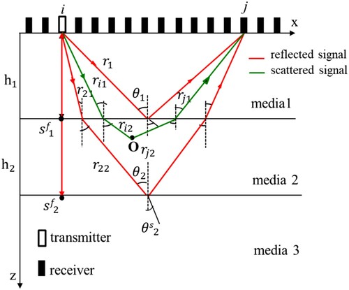
In case 2, for instance, the target located was in medium 2. The array element $i$ ($X_i$, 0) was assumed as the transmission source and emitted the signal $\Omega \left(t\right)$. The total signals recorded by the receiving array element $j$ ($X_j$, 0) could be expressed as: (1) $P_{ij}\left(t\right)=a_{ij}\Omega (t-t_0^{})+b_{ij}\Omega (t-{t_1}^{})+c_{ij}\Omega (t-{t_2}^{})$(1) where the first term refers to the signal scattered by the target through the interface, assuming a scattering coefficient of ${a_i}_j$ and travel time $t_0^{}=\frac{r_{i1}+r_{j1}}{c_1}+\frac{r_{i2}+r_{j2}}{c_2}$; the second and third terms are the signals reflected at S₁/S₂ interfaces with reflection coefficients $b_{ij}$, $c_{ij}$ and corresponding travel times $t_1^{}=\frac{2r_1}{c_1}$ and $t_2^{}=\frac{2r_{21}}{c_1}+\frac{2r_{22}}{c_2}$, respectively.

According to the mixed TR–RTM method, the array element emits a forward acoustic beam defined by: (2) $F_i\left(t\right)=\Omega \left(t\right)$(2)

The backward acoustic beam $R_{ij}\left(t\right)$ is the TR of the received signal and is emitted from array element $j$ ahead of time than the forward acoustic beam. The expression $\Delta T_0^{}$ is the travel time difference between the target scattering signal reaching the receiving array element and the transmitting signal reaching the target, i.e.$\Delta T_0^{}=(\frac{{r_{j1}}^{}}{c_1}+\frac{{r_{j2}}^{}}{c_2})-(\frac{{r_{i1}}^{}}{c_1}+\frac{{r_{i2}}^{}}{c_2})=t_0^{}-t_0^s/2$, as indicated in Figure 1. The expression $t_0^s$ is the travel time the signal is transmitted from the emitting array element scattered by the target and back to element $i$, which is equal to $\frac{\text{2}{r_{i1}}^{}}{c_1}+\frac{\text{2}{r_{i2}}^{}}{c_2}$. Thus, $t_0^{}$ and $t_0^s$ can be measured.

The backward acoustic beam is defined by: (3) $R_{ij}\left(t\right)=a_{ij}\left[\Omega \right(t-t_0^{}\text{ + }\Delta T_0^{}){]}^{\text{TR}}+b_{ij}\left[\Omega \right(t-{t_1}^{}\text{ + }\Delta T_0^{}){]}^{\text{TR}}+c_{ij}\left[\Omega \right(t-{t_2}^{}\text{ + }\Delta T_0^{}){]}^{\text{TR}}$(3)

Therefore, for any point $X(x,z)$ in space, the forward and reverse beams are convolved as: (4) $M_0(t,X)=F_i(t,X)\otimes R_{ij}(t,X)$(4) where $\otimes$ indicates that a convolution and a ridge-like distribution is formed. The ridge-top line is the maximum value of the convolution, inevitably passing the position of the target. For different emitter–receiver pairs, different ridge-like distributions are obtained; however, their ridge-top lines all pass the position of the target and form a common intersection point, i.e. the focus point. All throughout the emitter–receiver pairs, the convolution sum: (5) $M=\sum _{j=1}^n(F_1\otimes R_{1j}{)}_{max}$(5) is a superposition of several ridge-like destructions, which form a single and prominent mountain-like acoustic field distribution. The position of the summit is just the position of the target, thereby realizing the target detection and location.

The TR–RTM process was adopted formally for $S_1$ and $S_2$ (see Figure 1) interfaces, where the delay of its reverse beam were indicated by $\Delta T_{}^{s_1}=t_1-t_{{}_{s_1}}^s/2$ and $\Delta T_{}^{s_{\text{2}}}=t_{\text{2}}-t_{{}_{s_2}}^s/2$. Here, $t_{{}_{s_1}}^s$ and $t_{{}_{s_2}}^s$ refer to the respective travel times when the signal from an emitting element i was reflected by S₁/S₂ at reflection points $S_1^f$ and $S_2^f$, and back to element i. Moreover, t₁ and t₂ refer to the respective travel times when a signal was emitted by an $ith$ element and reflected by $S_1/S_2$ at reflection points $S_1$ and $S_2$, and arrived in the receiving element $j$. Because $S_1$ or $S_2$ and $S_1^f$ or $S_2^f$ (see Figure 1) were at different points on the interface, the convolution of the forward acoustic beam and the reverse acoustic beam formed a ridge-like distribution. However, such ridge-top lines did not appear at common intersections. After further superposition, a single and prominent mountain-like acoustic field distribution could not be formed, as it was merely a disordered and inhomogeneous acoustic field distribution with smaller amplitude. Through the TR–RTM process, the target and the interface can be distinguished, and the target can be located.

Similar results were obtained for a similar analysis in cases 1 and 3. In other words, the target was highlighted from multiple interface interferences, then detected and located in multilayered media.

3. Experimental research

The experimental arrangement of this paper is as follows:

1. Three-layered media of silicone rubber, gelatin, and water were prepared according to the relative parameters in Table 1. The targets were round steel bars with 2.5 mm of radius.

2. The PZT piezoelectric transducer array, consisting of 18 elements in total, was used. The elements were 1.8-mm wide and 0.8-mm thick, which correspond to a resonance frequency of 1 MHz. Each array element was used as a receiver, while the 10th array element was the transmitter. Figure 1 presents the schematic.

3. Measurement system: The signal generated by the signal source (TK-AFG3102) drove the transmitting element via a power amplifier (EI-2200L). An acoustic wave was generated and propagated into the media, and the received acoustic signal was displayed and recorded by a digital oscilloscope (TK-MDO3104) (Figure 2).

4. The transmitted signal exhibited the waveform, (6) $\Omega \text{(}t\text{)}=\left[H\left(t\right)-H\left(t-T/2\right)\right]\text{cos[}\omega (t-T/4\left)\right]\text{cos[}{\omega }_0\text{(}t-T/4\left)\right]$(6)

5. where the carrier signal is represented by ${\omega }_0=2\pi f_0$, $f_0=1\text{MHz}$. The modulated envelope signal was $\omega =\frac{2}{3}{\omega }_0$, $T=\frac{3}{2}\frac{1}{f_0}$, that is, the transmitted signal was a half-period modulated pulse with $f_0$.

6. Three cases were analyzed in the experiments: (a) Case 1: The upper medium was 70-mm-thick water; the middle layer 50-mm-thick gelatin and; the underlying medium was silicone rubber. Here, the target was placed in the upper medium (water) at position (20, 35 mm). Case 2: The upper medium was 50-mm-thick gelatin; the middle medium was 100-mm-thick water and; the bottom medium was silicone rubber. Here, the target was placed in the water medium at (20, 70 mm). Case 3: The upper medium was 50-mm-thick silicone rubber; the middle layer was 50-mm-thick gelatin and; the bottom medium was water. Here, the target was placed in the bottom water medium at (20 mm, 120 mm).

Figure 2. Signals received by the array element for (a) case 1, (b) case 2, and (c) case 3.

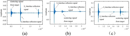
Table 1. Parameters of the layered media.

Medium	Material	Velocity (m s^–1)	Density (kg m^–3)	Thickness (mm)
Upper medium 1	Silicone rubber	1070	1096	50
Upper medium 2	Gelatin	1470	1047	50
Lower medium 1	Water	1500	1000	–

Travel times ($t_1^{}$, $t_2^{}$, and $t_0^{}$) and amplitudes $(a_{ij},b_{ij},c_{ij})$of the reflected signal at $S_1$ and $S_2$ interfaces and scattering signal of the target, were measured and recorded. The SIR of target and interfaces $S_1/S_2$ were provided.

Figure 2 describes a typical diagram for a signal received by the receiving array element in three cases. For all cases, the time sequence of the reflected signals at $S_1/S_2$ interfaces and the target-scattered signal as the reflected signal, defined the time difference, as shown in Figure 2(a–c). Figure 3 shows the ratio of the amplitude of the target-scattered signal and the interface-reflected signal of $S_1$ and $S_2$, which became the SIR interference.

Figure 3. SIR for different emitter–receiver pairs at $S_1$ interface for (a) case 1, (c) case 2, and (e) case 3, at $S_2$ interface for (b) case 1, (d) case 2, and (f) case 3, respectively.

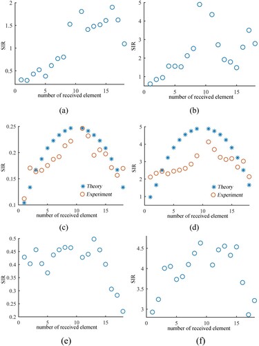
For case 2, the acoustic pressures of the reflecting interface and the scattering target were calculated theoretical, which were received by several receiving elements.

The $S_1$ interface-reflected acoustic pressure received at the $j\text{th}$ receiving element can be written expressed as (see Ref. [4] and Equation (2) in Ref [9]) (7) $p_r\cong \frac{A}{\sqrt{2k{r}_0}}\cdot \left(\frac{{\rho }_2{\text{c}}_2\cos {\theta }_1-{\rho }_1{\text{c}}_1\cos {\theta }_2}{{\rho }_2{\text{c}}_2\cos {\theta }_1+{\rho }_1{\text{c}}_1\cos {\theta }_2}\right){\left(\frac{\sin \left({\omega }_{0}d\sin {\theta }_1/c_1\right)}{{\omega }_{0}d\sin {\theta }_1/c_1}\right)}^2{e}^{2\text{j}\omega r_0/{\text{c}}_1}$(7)

Likewise, the $S_2$ interface-reflected acoustic pressure through interface $S_1$ at the receiving element can be written as [9] (8) $\begin{array}{rl}{p}_{r\text{2}}& \cong \frac{A\cdot e^{\text{2j}\omega \left(\frac{r_{\text{2}1}}{c_1}+\frac{r_{\text{2}2}}{c_2}\right)}}{k_1{r}_{i1}+\frac{k_2{r}_{i2}{\cos }^2{{\theta }^s}_{i1}}{{\cos }^2{{\theta }^s}_{i2}}}\left(\frac{2{\rho }_2{\text{c}}_2\cos {\theta }^s{{}_{i1}}_{}}{{\rho }_2{\text{c}}_2\cos {{\theta }^s}_{i1}+{\rho }_1{\text{c}}_1\cos {{\theta }^s}_{i2}}\right)\left(\frac{{\rho }_3{\text{c}}_3\cos {\theta }_2-{\rho }_2{\text{c}}_2\cos {{\theta }_2}^S}{{\rho }_3{\text{c}}_3\cos {\theta }_2+{\rho }_2{\text{c}}_2\cos {{\theta }_2}^S}\right)\\ & \ast \left(\frac{2{\rho }_{\text{1}}{\text{c}}_{\text{1}}\cos {{\theta }^s}_{i2}}{{\rho }_2{\text{c}}_2\cos {{\theta }^s}_{i1}+{\rho }_1{\text{c}}_1\cos {{\theta }^s}_{i2}}\right){\left(\frac{\sin \left({\omega }_{0}d\sin {{\theta }^s}_{i1}/c_1\right)}{{\omega }_{0}d\sin {{\theta }^s}_{i1}/c_1}\right)}^2\end{array}$(8)

The acoustic pressure of the acoustic beam scattered by the target through S₁ recorded in the $j\text{th}$ receiving element can be written as (see Equation 5 in Ref [9,10]) (9) $\begin{array}{rl}{p}_{st}& \cong \frac{A\sqrt{k_2{r}_{i2}}\cdot e^{\text{j}\omega \left(\frac{r_{j1}}{c_1}+\frac{r_{j2}}{c_2}\right)}}{\sqrt{k_1{r}_{i1}+\frac{k_2{r}_{i2}{\cos }^2{\theta }_{i1}}{{\cos }^2{\theta }_{i2}}}}\left(\frac{2{\rho }_1{\text{c}}_1\cos {\theta }_{j2}}{{\rho }_2{\text{c}}_2\cos {\theta }_{j1}+{\rho }_1{\text{c}}_1\cos {\theta }_{j2}}\right)\\ & \ast \sqrt{\frac{2a}{\pi r_{j2}}}\phi \left(\pi -({\theta }_{i2}+{\theta }_{i1})\right)\left(\frac{\sin \left({\omega }_{0}d\sin {\theta }_{j2}/c_2\right)}{{\omega }_{0}d\sin {\theta }_{j2}/c_2}\right)\end{array}$(9) where $a$ is the radius of the scatter, and $\phi \left(\varphi \right)$ is the directivity function of the scattered acoustic field [22].

According to Equations (7), (8), and (9), theoretical values of SIR of the target-scattered signals with $S_1/S_2$ interface-reflected signals, as shown in Figure 3(b,d), respectively, were in agreement with the experimental results.

4. TR–RTM processing

For the above cases, the measured data of target scattering signal and S1/S2 interface reflection signal were processed according to the hybrid TR–RTM method proposed in this paper.

For case2: The target was placed in the bottom medium, and its location was at (20, 70 mm). For $S_1/S_2$ interfaces, TR–RTM obtained an acoustic field distribution, as shown in Figure 4(a,b).

Figure 4. Results of the TR–RTM process for two interface-reflected signals (a) S1 and (b) S₂ in case 2.

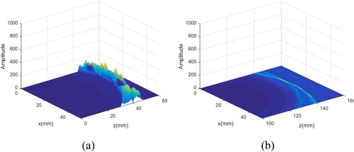
For $S_1/S_2$, a disordered and inhomogeneous acoustic field distribution with a smaller amplitude was formed, instead of a mountain-like acoustic field distribution (see in Figure 4(a,b)). Nevertheless, for the target scatter, TR–RTM obtained a signal and prominent mountain-like acoustic field distribution, where the measured position of the summit was nearer to the actual location of the target, as shown in Figure 5 and indicated in Table 2. Thus, detection and positioning of the target was realized.

Figure 5. Acoustic field (a) distribution map of the target signal in case 2.

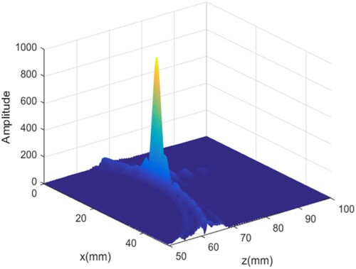
Table 2. Comparison of the measured and actual target positions.

Case	Actual position (x, z)	Measured position (x, z)
Case 1	20 mm, 35 mm	20.9, 34.8 mm
Case 2	20 mm, 70 mm	19.3, 68.8 mm
Case 3	20 mm, 120 mm	19.4, 118.3 mm

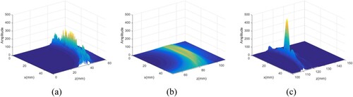
Figures 6 and 7 indicate similar results obtained for cases 1 and 3, where a single, prominent mountain-like acoustic field distribution was obtained around the target. The summit position agreed with actual position of target, whose values are listed in Table 2. Moreover, the reflected acoustic field distribution for interface $S_1/S_2$ was disordered and inhomogeneous, with smaller amplitude.

Figure 6. Results of the TR–RTM process of the target in the first layer medium in case 1. (a) The acoustic field distribution for the target signal. (b) and (c) the acoustic field distribution of interface S₁ and interface S₂, respectively.

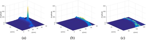
Figure 7. Results of the TR–RTM process of the target in the first layer medium. (a) and (b) the acoustic field distribution of interface $S_1$ and interface $S_2$, respectively, and (c) the acoustic field distribution for the target signal.

To further quantify the analysis of the effect of the TR–RTM method, the change in SIR before and after the implementation, was compared. On the one hand, the SIR before the process was defined as an average of the SIR of several elements shown in Figures 3 and 4. On the other hand, the SIR after the process was defined as the ratio of the peak value of the acoustic field distribution formed by the target scatter signal and the average value of the acoustic field distribution formed by the interface reflection signal, which were obtained in Figures 5–7. Table 3 summarizes the corresponding results.

Table 3. Signal-to-interference ratio (SIR) of target signal and interface reflection interference signal.

		Before processing	After processing	Multiple of increase
Case 1	Upper interface s1	1.1	7.6	6.3
	Lower interface s2	2.2	24.8	11.3
Case 2	Upper interface s1	1.0	4.2	4.2
	Lower interface s2	17.9	120.5	6.7
Case 3	Upper interface s1	0.4	2.1	5.3
	Lower interface s2	3.9	32.1	8.2

As Table 3 shows, the SIR greatly improved after the TR–RTM processing, indicating that the interference of the interface signal was better suppressed, thereby highlighting the target signal.

5. Conclusion

For media consisting of three or more layers, target detection and localization becomes more difficult due to the presence of a multilayer interface.

In this paper, the core idea of RTM is the principle of isochronism, which can not only deal with the target in multi-layer medium, but also deal with the interface by TR–RTM. Three cases were examined for target locations in medium 1, medium 2, or medium 3, respectively. For all cases after the TR–RTM process, a single and prominent peak-like acoustic field distribution was obtained for the target signal, and the location of the peak was the location of the target; therefore, detection and location of the target was realized. Moreover, the same method was applied to process the interface reflection signal. Due to the different positions of reflection points, the crest lines formed by different emission-receiving pairs intersect at different places, namely, there is no common intersection point. Therefore, SIR values were investigated for further quantitative analysis. Results indicated that the SIR after implementation of the TR–RTM process was much higher than that before the process. Moreover, the difference between the interface and the target was observed. In other words, through TR–RTM, the interface and target were distinguished, and target detection and localization in multilayered were simultaneously realized.

Note that fluid-fluid stratified media were the focus of this study. Our future work will investigate the more complex case of solid-fluid and solid–solid multilayer media.

Disclosure statement

No potential conflict of interest was reported by the author(s).

Additional information

Funding

This work is supported by National Natural Science Foundation of China [Grant Number 12004018 and 11772013], Project funded by China Postdoctoral Science Foundation [2019M660372], the State Key Laboratory of Acoustics, Chinese Academy of Sciences, Beijing Postdoctoral Research Foundation.

References

- Rose J L, Nagy PB. Ultrasonic waves in solid media. J Acoust Soc Am. 2000;107(4):1807–1808.
- Myers MR, Jorge AB, Mutton MJ, et al. A comparison of extended Kalman filter, ultrasound time-of-flight measurement models for heating source localization. Inverse Probl Sci Eng. 2012;2012(7):991–1016.
- Vorovich II, Boyev NV, Sumbatyan MA. Reconstruction of the obstacle shape in acoustic medium under ultrasonic scanning. Inverse Probl Sci Eng. 2001;9(4):315–337.
- Kari M, Honarvar F. Nondestructive characterization of materials by inversion of acoustic scattering data. Inverse Probl Sci Eng. 2014;22(5):814–831.
- Seyedpoor SM, Ahmadi A, Pahnabi N. Structural damage detection using time domain responses and an optimization method. Inverse Probl Sci Eng. 2018;27(2):1–20.
- Jakubczak P, Nardi D, Bienia J, et al. Non-destructive testing investigation of gaps in thin glare laminates. Nondestr Test Eval. 2019;2019(1):1–18.
- Michalcová L, Hron R. Quantitative Evaluation of Delamination in Composites Using Lamb Waves. IOP Conf Ser: Mater Sci Eng. 2018;326(1):1–6.
- Cunningham LJ, Mulholland AJ, Tant KMM, et al. A spectral method for sizing cracks using ultrasonic arrays. Inverse Probl Sci Eng. 2017;25(12):1788–1806.
- Messineo MG, Frontini GL, Eliçabe GE, et al. Equivalent ultrasonic impedance in multilayer media. A parameter estimation problem. Inverse Probl Sci Eng. 2013;21(8):1268–1287.
- Fink M, Prada C, Wu F, et al. Self focusing in inhomogeneous media with time reversal acoustic mirrors. IEEE Ultrasonics Symposium; IEEE; 1989. p. 681–686.
- Chakroum N, Fink M, Wu F. Time reversal processing in ultrasonic nondestructive testing. IEEE Trans Ultrason Ferroelectr Freq Control. 1995;42(6):1087–1098.
- Etgen J, Gray SH, Zhang Y. An overview of depth imaging in exploration geophysics.. Geophysics. 2009;74(6):WCA5-17.
- Lerosey G, De Rosny J, Tourin A, et al. Time reversal of electromagnetic waves. Phys Rev Lett. 2004;92(19):193904.
- Wei W, Wang CH. Self-adaptive focusing by time reversal through interface between different media. Chin J Acoust. 2000;19(1):83–88.
- Baysal JF, Kosloff DO, Sherwood JWC. A two-way nonreflecting wave equation. Geophysics. 1984;49(2):132–141.
- Shi FF, Wang CH, Zhang BX, et al. Acoustic detection and location of targets in layered media by a mixed method of time reversal and reverse time migration. Chin J Acoust. 2013;38(6):639–647.
- Gao X, Li J, Shi FF, et al. Acoustic analysis of detection and location of targets in layered media by time reversal-reverse time migration mixed method. Chin J Acoust. 2017;36(4):385–400.
- Tant KMM, Galetti E, Mulholland AJ, et al. Effective grain orientation mapping of complex and locally anisotropic media for improved imaging in ultrasonic non-destructive testing. Inverse Probl Sci Eng. 2020;28(12):1–25.
- Gao X, Li J, Ma J, et al. Experimental investigation of the detection and location of a target in layered media by using the TR–RTM mixed method. Mech Astron. 2019;62(3):1–7.
- Morse PM. Vibration and sound. New York (NY): McGraw-Hill; 1948.
- Assous F, Lin M. Time reversal for elastic scatterer location from acoustic recording. J Comput Phys. 2020;423:109786.
- Hong M, Su ZQ, Lu Y, et al. Locating fatigue damage using temporal signal features of nonlinear lamb waves. Mech Syst Sig Process. 2015;60:182–197.
- Gao X, Li J, Shi FF, et al. Weighting technique for detection and location of targets by TR-RTM mixed method. Symposium on Piezoelectricity, Acoustic Waves and Device Applications; 2018; Chengdu, China.
- Aram M G, Haghparast M, Abrishamian M S, et al. Comparison of imaging quality between linear sampling method and time reversal in microwave imaging problems. Inverse Probl Sci Eng. 2016;24(7):1347–1363.
- Lobato FS, Steffen Jr V, Silva Neto AJ. Solution of inverse radiative transfer problems in two-layer participating media with differential evolution. Inverse Probl Sci Eng. 2010;18(2):183–195.
- Yu C, Ma S, Fu L, et al. Passive localization techniques of a vector hydrophone based on time-reversal method. IEEE/OES Acoustics in Underwater Geosciences Symposium; 2013 July 24–26; Rio de Janeiro, Brazil. IEEE.
- Wang WW, Hong JS, Zhang GM, et al. Node localization based on time reversal in wireless sensor network. International conference on Microwave and Millimeter Wave Technology; 2010 May 8–11; Chengdu, China. IEEE.