Bayesian damage identification of simply supported beams from elastostatic data

Abstract

This paper considers a statistical method for damage identification of simply-supported elastic beams from static data. The problem is cast as an inverse problem and analyzed in Bayesian inversion framework. The main goal is to obtain a probabilistic model for the spatial distribution of the damage across a beam given limited and noisy data on the static beam response. A principal distinction of the proposed method is its ability to identify not only an estimate of the damage occurred to the beam but also the uncertainty (error) associated with such an estimate. Moreover, the proposed method uses simple static data instead of dynamic or spectral data, unlike the majority of research work published in the literature. This is a challenge as static data is a rather limited source of information about the underlying physical system compared to dynamic data. Finally, the proposed method does not involves any computationally expensive high-dimensional integration algorithms unlike the existing methods. According to the numerical analysis conducted in this paper, the result obtained by using the proposed damage identification method lies within one standard deviation interval.

Keywords:

• Inverse problems
• Bayesian statistics
• damage identification
• elasticity
• beams
• static data

2010 Mathematics Subject Classifications:

• 62F15
• 34A55
• 74G75
• 74J25
• 74R99

1. Introduction

Modeling and analysis of elastic deformation [1] has led to many challenging problems in computational elasticity since the advent of modern computing. In general, there are two different classes of computational elasticity problems: forward and inverse problems [2,3]. In forward problems, the mechanical parameters characterizing the continuum body along with all the external variables including the external force and boundary conditions are given but the deformation is unknown. In inverse problems [4], the unknown includes some mechanical parameters or external variables while the deformation and the other parameters and variables are partially known or measured. When the unknown is the external force applied to the body, the relevant inverse problem is a force reconstruction problem [5–13]. When the unknown relates to the boundary conditions of the problem, the problem is a boundary value identification problem, also known as the inverse boundary problem [14]. When the unknown includes some parameters related to the mechanical or geometrical characteristics of the body, the problem is a coefficient identification problem [15–21].

Usually, a force reconstruction problem can be studied as a de-convolution problem [22,23]; which is a common problem in the theory of inverse problems. However, a coefficient identification problem is rather more complicated. An important subgroup of coefficient identification problems is usually referred to as the damage identification problems [24–30]. In this paper, we consider a damage identification problem for simply-supported elastic beams when the damage affects the mechanical properties of (a subdomain of) the body.

An approach to classify damage identification problems in computational elasticity is based on the characteristics of the deformation occurred to the continuum body of interest. Both dynamic and static damage identification problems are based on the fact that dynamic or static characteristics of the deformation are directly related to the mechanical properties of the underlying physical system; therefore, a change in these characteristics may indicate a possible damage [31–33]. When the deformation is vibrational, the given data usually includes either a vector-valued time series relating to the vibrational deformation of the body or modal characteristics of the vibration such as natural frequencies and mode shapes. In this case, the damage identification problem is a dynamic problem [5,34–40]. In several practical cases, a static load is easier to arrange than a (controlled) dynamic load. In this case the deformation is static and the given data usually includes only a single vector-valued variable relating to the elastostatic deformation of the body at a number of locations. In this case, the damage identification problem is a static problem. This problem has been investigated by various researchers [28,29,41–44]; however, the existing literature on this problem is relatively poor compared to the literature on dynamic damage identification. Obviously, static damage identification problems are more challenging as static data is a rather limited source of information about the underlying physical system when compared to vibrational data [45,46]. In this paper, we consider static data to analyze damage identification problem of structural beams.

Damage identification problems can be also classified based on the inversion framework used for their analyzes. When the unknown is taken to be a deterministic variable, the regularization framework is usually used [47,48]. In this framework, the error is taken to be unknown and not specifically with any probabilistic structure; however, it is often assumed that the error norm is known. The inverse problems that are cast in this framework are called deterministic inverse problems. These problems are often solved as optimization problems. When the unknown, modeling error and measurement error are explicitly taken and modeled as jointly distributed random variables, statistical or Bayesian framework should be used. The inverse problems that are cast in this framework are called Bayesian inverse problems [4,49,50]. These problems can be solved for not only an estimate of the unknown but also statistically meaningful uncertainty of the estimates [50]. In this paper, we consider Bayesian inversion framework.

The scope of this paper is damage identification problem for structural elements that can be modeled as beams by using either Euler-Bernoulli or Timoshenko beam theories. Some simplified versions of this problem have been investigated in the literature by using deterministic inversion framework [15–21]. However, this paper considers Bayesian inversion framework to estimate not only the occurred damage but also its uncertainty for the structures of interest. The rest of this paper is organized as follows. Section 2 gives a brief literature review on the research field. Section 3 develops a finite-dimensional model relating a finite-dimensional representation of the static beam response to a finite-dimensional representation of the occurred damage field. In this section, both Timoshenko and Euler-Bernoulli beam models are considered. Section 4 discusses a framework for the generation of random damage fields and proposes a probabilistic model for such fields. Section 5 analyzes the problem in Bayesian inversion framework and calculates a posterior density for the damage field given limited and noisy data. This section is followed by the derivation of a point estimate and modeling its uncertainty. Section 6 elaborates a set of numerical results verifying the validity and efficiency of the proposed method. Finally, Section 7 gives concluding remarks and discusses future work.

2. Literature review on damage identification of elastic beams

One of the first studies casting beam identification as a computational inverse problem was published in [51]. In this study, the beam identification problem was formulated as finding the spatial distribution of some coefficients used for modeling the beam, denoted by $\beta (x)\in \mathbb{R}$ hereafter, given some limited data on the dynamic beam response, denoted by $\mathbf{d}{\in \mathbb{R}}^m$ hereafter. The Euler-Bernoulli beam theory was used to find a computational model, mapping a finite-dimensional representation of $\beta (x)$ to $\mathbf{d}$. This mapping is usually referred to as the forward model in the theory of inverse problems. Tikhonov Regularization method [47] was then applied to solve the inverse problem associated with the forward model. The same problem was later studied in [24] but considering the Timoshenko beam theory. Both the studies published in [51] and [24] used the deterministic inversion framework to find estimates of $\beta (x)$ without determining the uncertainty associated with such estimates. In general this issue can be addressed by using statistical or Bayesian inversion frameworks.

There has been relatively little literature published on the application of the Bayesian framework for the beam coefficient or damage identification problems. The relevant research to date has tended to focus on the crack identification problem (a very special case of the damage identification problem), which is to estimate a probabilistic model for only the location, length and depth of the crack(s) when the existence of the crack(s) is known and the rest of the beam is assumed to be undamaged [27,52–55]. For example, the Bayesian framework was used to study the crack identification problem of Euler-Bernoulli beams in [27]. This framework was also used to study the crack identification problem of Timoshenko beams in [52] and [56]. One common characteristic of these studies is their need to measure the natural frequencies of the dynamic beam response. Also, these studies suffer from high computational complexity due to the non-linear relation between the crack parameters and the natural frequencies. A further study based on the statistical damage identification of a spacial case of Euler-Bernoulli beam was published in [57]. In this paper, a single crack was modeled by using a V-shaped notch and the data collected from the dynamic beam response was used to identify the parameters of the V-shaped notch. The uncertainty of the estimated solution was also calculated. A computationally expensive algorithm based on Markov Chain Monte Carlo algorithm was used to deal with the high-dimensional integration and the non-linear relation between the data and crack parameters. More recently, the Bayesian damage identification of thick beams (2D) was reported in [25] based on dynamic data. In this study, the partial recovery of the damage field was performed from the use of the Timoshenko beam model (1D) adopting the Bayesian approximation error (BAE) approach to build a statistical model for the model discrepancy.

In all the Bayesian identification studies mentioned above, the identification algorithm uses the dynamic beam response. However, in some practical applications, the external force or load applied to the beam is static and the dynamic beam response is not available. Beam coefficient identification from elastostatic response was studied in [15]. In this paper, the Euler-Bernoulli beam theory was used to formulate the problem as an extension to the coefficient identification problem of the Poisson equation. The existence and uniqueness of the solution with different boundary conditions was proved. As a practical example, a specific solution for simply-supported boundary conditions was derived. The spatial distribution of the beam coefficient $\beta (x)$ was modeled by a piece-wise constant function with discrete levels ${\beta }_1,\dots ,{\beta }_n$ at the consecutive intervals ${\mathrm{\Omega }}_1\dots ,{\mathrm{\Omega }}_n$ dividing the beam into n equal elements. Then, a computational forward model, mapping $[{\beta }_1,\dots ,{\beta }_n{]}^{\mathrm{T}}$ into a vector formed by the measured data was developed. Tikhonov Regularization technique [47] was used to solve the inverse problem associated with the forward model. The accuracy of the proposed solution was shown through an example in which $\beta (x)$ is a smooth function, and the data SNR is very high (only 1% noise). The same problem was studied in [18] but the Method of Variational Imbedding (MVI) was used as the regularization method. Similar to [15], $\beta (x)$ was modeled by a piece-wise constant function and the accuracy of the proposed solution was shown through a simple example when $\beta (x)$ was a smooth function over the beam, and the data supposed to be noise-free. The studies presented in [19] extended the one presented in [18] by considering piece-wise linear and piece-wise cubic models for $\beta (x)$.

Beam damage identification from limited data on the static beam response was studied in [29]. In this study, a homogeneous undamaged beam with a constant parameter ${\beta }_0\in \mathbb{R}$ was considered. The coefficient of the damaged beam was modeled as the product of ${\beta }_0$ and $1-D(x)$, where $0\le D(x)<1$ was a function indicating the spatial distribution of the damage across the beam. The beam was divided into n equal intervals and it was supposed that $D(x)$ is constant over each interval. The Euler-Bernoulli beam theory and Direct Stiffness Method [58] were used to obtain a computational forward model, mapping the constant levels of $D(x)$ at each interval into a vector formed by the measured data. Tikhonov Regularization [47] was then used to solve the associated inverse problem. A cantilever beam was considered, but the method could be adopted for simply-supported beams as well. Most recently, the same problem was studied for different boundary conditions including simply-supported boundary conditions in [28]. In this study, the damage across an Euler-Bernoulli beam was estimated through the minimization of an error (measure) called the constitutive relation error. This study considered the effect of the measurement noise statistics on the estimated solution; but it used a deterministic inversion approach.

2.1. Classification of existing methods

The above-mentioned studies can be categorized by using three different classification approaches. (1) the type of beam response used as the input data, which could be either dynamic or static. (2) the beam theory used for developing the forward model, which could be either the Euler-Bernoulli or Timoshenko beam theory, and (3) the inversion method used for solving the inverse problem, which could be either deterministic or probabilistic.

Based on these classification criteria, we can classify these studies as shown in Table 1. According to this table, all the relevant studies to date, that use the data collected from the static beam response, are based on deterministic inversion framework. They usually find an approximate solution for the unknown, without assessing the uncertainty of the solution. To the best of our knowledge, for distributed damage, there is no substantial research on the Bayesian coefficient identification or damage identification of beams from the static response data (elastostatic data) based on either Euler-Bernoulli or Timoshenko beam theories, as shown in Table 1. The main motivation of this paper is to address this research gap for simply-supported beams considering both Euler-Bernoulli and Timoshenko beam models.

Table 1. Classification of existing works on damage identification of simply-supported beams.

	Deterministic inversion		Probabilistic inversion
	Euler-Bernoulli model	Timoshenko model	Euler-Bernoulli model	Timoshenko model
Dynamic response	Smith et al. [51]	Karve et al. [24]	Ng et al. [27]	Shuai He et al. [56]
			Teixeira et al. [57]	Others [53,54]
Static response	Lesnic et al. [15]	None	This Paper	This Paper
	Marinov et al. [18]
	Ghrib et al. [29]
	Guo et al. [28]

3. Derivation of computational forward model

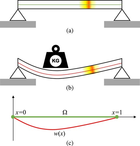
Figure 1 shows the transverse section of a damaged simply-supported beam whose neutral axis lies on the x-axis. Figure 1(a) shows the beam position when there is no external force. Figure 1(b) shows the deformation of the beam when a transverse force is applied; the beam neutral axis after deformation is also shown. Figure 1(c) shows the beam neutral axis, denoted by Ω, before and after deformation in a single coordinate system. As shown in Figure 1, the beam boundaries are pinned (simply-supported boundary conditions). In this situation, the deflection and bending moments are always zero at the boundary points. In this paper, we consider a static profile for the external force and refer to the beam deflection or deformation as the static beam response. Referring to Figure 1(c), the beam static response can be modeled by using Timishenko beam theory as follows: (1) $\{\begin{array}{l}{\beta }_0{\displaystyle \frac{{\mathrm{d}}^2}{\mathrm{d}{x}^2}}\{\lambda (x){\displaystyle \frac{{\mathrm{d}}^2}{\mathrm{d}{x}^2}}w(x)-k_0\lambda (x){\displaystyle \frac{\mathrm{d}}{\mathrm{d}x}}\left\{{\displaystyle \frac{Q(x)}{\lambda (x)}}\right\}\}=f(x)\\ {\displaystyle \frac{\mathrm{d}}{\mathrm{d}x}}Q(x)=-f(x)\end{array}x\in \mathrm{\Omega }$(1) where $\mathrm{\Omega }=[0,1]$ is the beam neutral axis, $w(x):\mathrm{\Omega }\to \mathbb{R}$ is the static beam response, $f(x):\mathrm{\Omega }\to \mathbb{R}$ is the external transverse force, $Q(x):\mathrm{\Omega }\to \mathbb{R}$ is the shear force, ${\beta }_0\in \mathbb{R}$ is the bending stiffness of the undamaged beam and $k_0\in \mathbb{R}$ is shear compliance of the undamaged beam. In this model, $0<\lambda (x)\le 1$ represents the damage field; this function is related to the links among material points and can be interpreted as a measure of local cohesion or integrity state of the continuum body [59]. For this function, the maximum value of 1 indicates that the continuum body is undamaged and the infimum value of 0 indicates a local rupture in the continuum body. The thermodynamic framework used to obtain the modified constitutive relation is not within the scope of this paper. Further information can be found in [59–61]. As mentioned earlier, the beam deflection and bending moment, are zero at the boundary points of a simply-supported beam; hence, the solution of (1(1) $\{\begin{array}{l}{\beta }_0{\displaystyle \frac{{\mathrm{d}}^2}{\mathrm{d}{x}^2}}\{\lambda (x){\displaystyle \frac{{\mathrm{d}}^2}{\mathrm{d}{x}^2}}w(x)-k_0\lambda (x){\displaystyle \frac{\mathrm{d}}{\mathrm{d}x}}\left\{{\displaystyle \frac{Q(x)}{\lambda (x)}}\right\}\}=f(x)\\ {\displaystyle \frac{\mathrm{d}}{\mathrm{d}x}}Q(x)=-f(x)\end{array}x\in \mathrm{\Omega }$(1) ) should satisfy the following boundary conditions: (2) $\{\begin{array}{l}w(0)=w(1)=0\\ M(0)=M(1)=0\end{array}$(2) where $M(x)$ representing the beam bending moment is given by (3) $M(x)=-{\beta }_0\lambda (x)\frac{{\mathrm{d}}^2}{\mathrm{d}{x}^2}w(x)+{\beta }_0{k}_0\lambda (x)\frac{\mathrm{d}}{\mathrm{d}x}\left\{\frac{Q(x)}{\lambda (x)}\right\}$(3) To obtain a computational forward model, we could apply the Galerkin Approximation Method (GAM) directly to (1(1) $\{\begin{array}{l}{\beta }_0{\displaystyle \frac{{\mathrm{d}}^2}{\mathrm{d}{x}^2}}\{\lambda (x){\displaystyle \frac{{\mathrm{d}}^2}{\mathrm{d}{x}^2}}w(x)-k_0\lambda (x){\displaystyle \frac{\mathrm{d}}{\mathrm{d}x}}\left\{{\displaystyle \frac{Q(x)}{\lambda (x)}}\right\}\}=f(x)\\ {\displaystyle \frac{\mathrm{d}}{\mathrm{d}x}}Q(x)=-f(x)\end{array}x\in \mathrm{\Omega }$(1) )–(3(3) $M(x)=-{\beta }_0\lambda (x)\frac{{\mathrm{d}}^2}{\mathrm{d}{x}^2}w(x)+{\beta }_0{k}_0\lambda (x)\frac{\mathrm{d}}{\mathrm{d}x}\left\{\frac{Q(x)}{\lambda (x)}\right\}$(3) ); however, this approach would result in a non-linear forward model. Furthermore, this approach would require a set of basis functions in $C^3(\mathrm{\Omega })$, e.g. cubic Hermite functions. To avoid these consequences, we exploit a different modeling approach in this paper. We first develop an alternative formulation for (1(1) $\{\begin{array}{l}{\beta }_0{\displaystyle \frac{{\mathrm{d}}^2}{\mathrm{d}{x}^2}}\{\lambda (x){\displaystyle \frac{{\mathrm{d}}^2}{\mathrm{d}{x}^2}}w(x)-k_0\lambda (x){\displaystyle \frac{\mathrm{d}}{\mathrm{d}x}}\left\{{\displaystyle \frac{Q(x)}{\lambda (x)}}\right\}\}=f(x)\\ {\displaystyle \frac{\mathrm{d}}{\mathrm{d}x}}Q(x)=-f(x)\end{array}x\in \mathrm{\Omega }$(1) ) based on splitting it into two second-order sub-models. Then we apply the GAM to each sub-model separately. This process leads to a linear model. Furthermore, since the sub-models are formulated by second-order differential equations, we can use a simple set of basis functions in $C^1(\mathrm{\Omega })$, e.g. hat functions. A similar idea of splitting the Euler-Bernoulli beam model into two second-order sub-models was introduced in [15] and [16]. In fact, we generalize this idea in this paper so that we can use it for both Timoshenko and Euler-Bernoulli beam models. Let us define (4) $u(x)\triangleq \frac{1}{\gamma (x)}\frac{{\mathrm{d}}^2}{\mathrm{d}{x}^2}w(x)-\frac{k_0}{\gamma (x)}\frac{\mathrm{d}}{\mathrm{d}x}\{\gamma (x)Q(x)\}$(4) where (5) $\gamma (x)=\frac{1}{\lambda (x)}$(5) Since (5(5) $\gamma (x)=\frac{1}{\lambda (x)}$(5) ) is a one-to-one relation when $\lambda (x)\ne 0$, we can find the damage field $\lambda (x)$ from $\gamma (x)$ and vice versa. Since $0<\lambda (x)\le 1$; (5(5) $\gamma (x)=\frac{1}{\lambda (x)}$(5) ) leads to (6) $\gamma (x)\ge 1$(6) The change of variables given in (5(5) $\gamma (x)=\frac{1}{\lambda (x)}$(5) ) results in a linear mapping between the unknown and data variables of the proposed analysis. By substituting (4(4) $u(x)\triangleq \frac{1}{\gamma (x)}\frac{{\mathrm{d}}^2}{\mathrm{d}{x}^2}w(x)-\frac{k_0}{\gamma (x)}\frac{\mathrm{d}}{\mathrm{d}x}\{\gamma (x)Q(x)\}$(4) ) into (1(1) $\{\begin{array}{l}{\beta }_0{\displaystyle \frac{{\mathrm{d}}^2}{\mathrm{d}{x}^2}}\{\lambda (x){\displaystyle \frac{{\mathrm{d}}^2}{\mathrm{d}{x}^2}}w(x)-k_0\lambda (x){\displaystyle \frac{\mathrm{d}}{\mathrm{d}x}}\left\{{\displaystyle \frac{Q(x)}{\lambda (x)}}\right\}\}=f(x)\\ {\displaystyle \frac{\mathrm{d}}{\mathrm{d}x}}Q(x)=-f(x)\end{array}x\in \mathrm{\Omega }$(1) ), we obtain (7) ${\beta }_0\frac{{\mathrm{d}}^2}{\mathrm{d}{x}^2}u(x)=f(x)x\in \mathrm{\Omega }$(7) The comparison of (3(3) $M(x)=-{\beta }_0\lambda (x)\frac{{\mathrm{d}}^2}{\mathrm{d}{x}^2}w(x)+{\beta }_0{k}_0\lambda (x)\frac{\mathrm{d}}{\mathrm{d}x}\left\{\frac{Q(x)}{\lambda (x)}\right\}$(3) ) and (4(4) $u(x)\triangleq \frac{1}{\gamma (x)}\frac{{\mathrm{d}}^2}{\mathrm{d}{x}^2}w(x)-\frac{k_0}{\gamma (x)}\frac{\mathrm{d}}{\mathrm{d}x}\{\gamma (x)Q(x)\}$(4) ) shows that $M(x)=-{\beta }_{0}u(x)$; thus, the boundary conditions given in (2(2) $\{\begin{array}{l}w(0)=w(1)=0\\ M(0)=M(1)=0\end{array}$(2) ) leads to $u(0)=0$ and $u(1)=0$. Therefore, $u(x)$ is modeled by the following boundary value problem: (8) ${\mathcal{M}}_1:\{\begin{array}{ll}{\beta }_0{\displaystyle \frac{{\mathrm{d}}^2}{\mathrm{d}{x}^2}}u(x)=f(x)& x\in \mathrm{\Omega }\\ u(0)=u(1)=0& \end{array}$(8) Now, we rearrange (4(4) $u(x)\triangleq \frac{1}{\gamma (x)}\frac{{\mathrm{d}}^2}{\mathrm{d}{x}^2}w(x)-\frac{k_0}{\gamma (x)}\frac{\mathrm{d}}{\mathrm{d}x}\{\gamma (x)Q(x)\}$(4) ) to write (9) $\frac{{\mathrm{d}}^2}{\mathrm{d}{x}^2}w(x)=\gamma (x)u(x)+k_0\frac{\mathrm{d}}{\mathrm{d}x}\{\gamma (x)Q(x)\}$(9) The shear force and bending moments satisfy $Q(x)=-\frac{\mathrm{d}}{\mathrm{d}x}M(x)$; therefore, from (3(3) $M(x)=-{\beta }_0\lambda (x)\frac{{\mathrm{d}}^2}{\mathrm{d}{x}^2}w(x)+{\beta }_0{k}_0\lambda (x)\frac{\mathrm{d}}{\mathrm{d}x}\left\{\frac{Q(x)}{\lambda (x)}\right\}$(3) ) and (4(4) $u(x)\triangleq \frac{1}{\gamma (x)}\frac{{\mathrm{d}}^2}{\mathrm{d}{x}^2}w(x)-\frac{k_0}{\gamma (x)}\frac{\mathrm{d}}{\mathrm{d}x}\{\gamma (x)Q(x)\}$(4) ) we obtain (10) $Q(x)=-{\beta }_0\frac{\mathrm{d}}{\mathrm{d}x}u(x)$(10) By substituting (10(10) $Q(x)=-{\beta }_0\frac{\mathrm{d}}{\mathrm{d}x}u(x)$(10) ) into (9(9) $\frac{{\mathrm{d}}^2}{\mathrm{d}{x}^2}w(x)=\gamma (x)u(x)+k_0\frac{\mathrm{d}}{\mathrm{d}x}\{\gamma (x)Q(x)\}$(9) ), we obtain (11) $\frac{{\mathrm{d}}^2}{\mathrm{d}{x}^2}w(x)=p(x)$(11) where (12) $p(x)=\gamma (x)u(x)-{\beta }_0{k}_0\frac{\mathrm{d}}{\mathrm{d}x}\{\gamma (x)\frac{\mathrm{d}}{\mathrm{d}x}u(x)\}$(12) From (2(2) $\{\begin{array}{l}w(0)=w(1)=0\\ M(0)=M(1)=0\end{array}$(2) ), we have $w(0)=0$ and $w(1)=0$. Therefore, we can write the following boundary value problem for $w(x)$: (13) ${\mathcal{M}}_2:\{\begin{array}{ll}{\displaystyle \frac{{\mathrm{d}}^2}{\mathrm{d}{x}^2}}w(x)=p(x)& x\in \mathrm{\Omega }\\ w(0)=w(1)=0& \end{array}$(13) Thus, the fourth-order model given by (1(1) $\{\begin{array}{l}{\beta }_0{\displaystyle \frac{{\mathrm{d}}^2}{\mathrm{d}{x}^2}}\{\lambda (x){\displaystyle \frac{{\mathrm{d}}^2}{\mathrm{d}{x}^2}}w(x)-k_0\lambda (x){\displaystyle \frac{\mathrm{d}}{\mathrm{d}x}}\left\{{\displaystyle \frac{Q(x)}{\lambda (x)}}\right\}\}=f(x)\\ {\displaystyle \frac{\mathrm{d}}{\mathrm{d}x}}Q(x)=-f(x)\end{array}x\in \mathrm{\Omega }$(1) )–(3(3) $M(x)=-{\beta }_0\lambda (x)\frac{{\mathrm{d}}^2}{\mathrm{d}{x}^2}w(x)+{\beta }_0{k}_0\lambda (x)\frac{\mathrm{d}}{\mathrm{d}x}\left\{\frac{Q(x)}{\lambda (x)}\right\}$(3) ) can be represented by two coupled second-order sub-models ${\mathcal{M}}_1$ and ${\mathcal{M}}_2$ given by (8(8) ${\mathcal{M}}_1:\{\begin{array}{ll}{\beta }_0{\displaystyle \frac{{\mathrm{d}}^2}{\mathrm{d}{x}^2}}u(x)=f(x)& x\in \mathrm{\Omega }\\ u(0)=u(1)=0& \end{array}$(8) ) and (13(13) ${\mathcal{M}}_2:\{\begin{array}{ll}{\displaystyle \frac{{\mathrm{d}}^2}{\mathrm{d}{x}^2}}w(x)=p(x)& x\in \mathrm{\Omega }\\ w(0)=w(1)=0& \end{array}$(13) ). The forward problem of ${\mathcal{M}}_1$ is to find $u(x)$ given ${\beta }_0$ and $f(x)$. From (7(7) ${\beta }_0\frac{{\mathrm{d}}^2}{\mathrm{d}{x}^2}u(x)=f(x)x\in \mathrm{\Omega }$(7) ), it is evident that $u(x)$ is not related to health or damage conditions of the beam. The forward problem of ${\mathcal{M}}_2$ is to find the beam response, $w(x)$, given $p(x)$. We can use (12(12) $p(x)=\gamma (x)u(x)-{\beta }_0{k}_0\frac{\mathrm{d}}{\mathrm{d}x}\{\gamma (x)\frac{\mathrm{d}}{\mathrm{d}x}u(x)\}$(12) ) to obtain $p(x)$ from ${\beta }_0$, $k_0$, $\gamma (x)$ and the obtained solution for $u(x)$. Obviously, $w(x)$ is related to the beam health or damage conditions.

Figure 1. Static response of a simply-supported beam, (a): beam and its neutral axis (b): static deformation due to external force, (c): neutral axis before and after deformation

3.1. Weak solution for beam static response

Let us first consider the forward problem of ${\mathcal{M}}_1$, which is to find $u(x)$ given ${\beta }_0$ and $f(x)$. Here we consider ${\beta }_0>0$ and $f(x)\in L^2(\mathrm{\Omega })$ based on the physical conditions of the problem. In this case, a function $u(x)\in C_0^2(\mathrm{\Omega })$ satisfying (8(8) ${\mathcal{M}}_1:\{\begin{array}{ll}{\beta }_0{\displaystyle \frac{{\mathrm{d}}^2}{\mathrm{d}{x}^2}}u(x)=f(x)& x\in \mathrm{\Omega }\\ u(0)=u(1)=0& \end{array}$(8) ) is a classical solution of the forward problem of ${\mathcal{M}}_1$. After multiplying both sides of the differential equation of ${\mathcal{M}}_1$ by a test function $v(x)\in C_0^2(\mathrm{\Omega })$, integrating over Ω, and using integration by parts, we can obtain (14) ${\beta }_0{[v(x)\frac{\mathrm{d}}{\mathrm{d}x}u(x)]}_0^1-{\beta }_0{\int }_{\mathrm{\Omega }}(\frac{\mathrm{d}}{\mathrm{d}x}v(x))(\frac{\mathrm{d}}{\mathrm{d}x}u(x))\mathrm{d}x={\int }_{\mathrm{\Omega }}v(x)f(x)\mathrm{d}x$(14) Since $v(x)$ vanishes at the boundary points of Ω, (14(14) ${\beta }_0{[v(x)\frac{\mathrm{d}}{\mathrm{d}x}u(x)]}_0^1-{\beta }_0{\int }_{\mathrm{\Omega }}(\frac{\mathrm{d}}{\mathrm{d}x}v(x))(\frac{\mathrm{d}}{\mathrm{d}x}u(x))\mathrm{d}x={\int }_{\mathrm{\Omega }}v(x)f(x)\mathrm{d}x$(14) ) is simplified to (15) $-{\beta }_0{\int }_{\mathrm{\Omega }}(\frac{\mathrm{d}}{\mathrm{d}x}v(x))(\frac{\mathrm{d}}{\mathrm{d}x}u(x))\mathrm{d}x={\int }_{\mathrm{\Omega }}v(x)f(x)\mathrm{d}x$(15) A function $u(x)\in H_0^1(\mathrm{\Omega })$ satisfying (15(15) $-{\beta }_0{\int }_{\mathrm{\Omega }}(\frac{\mathrm{d}}{\mathrm{d}x}v(x))(\frac{\mathrm{d}}{\mathrm{d}x}u(x))\mathrm{d}x={\int }_{\mathrm{\Omega }}v(x)f(x)\mathrm{d}x$(15) ) and the boundary conditions of ${\mathcal{M}}_1$, i.e. $u(1)=u(0)=0$, for all $v(x)\in H_0^1(\mathrm{\Omega })$, is called a weak solution for the forward problem of ${\mathcal{M}}_1$. Also, the integral equation given in (15(15) $-{\beta }_0{\int }_{\mathrm{\Omega }}(\frac{\mathrm{d}}{\mathrm{d}x}v(x))(\frac{\mathrm{d}}{\mathrm{d}x}u(x))\mathrm{d}x={\int }_{\mathrm{\Omega }}v(x)f(x)\mathrm{d}x$(15) ) is called the weak form of the problem. Now, let us define a linear form (16) $l(v)={\int }_{\mathrm{\Omega }}v(x)f(x)\mathrm{d}x$(16) and a bi-linear form (17) $\mathcal{B}(v,u)=-{\beta }_0{\int }_{\mathrm{\Omega }}(\frac{\mathrm{d}}{\mathrm{d}x}v(x))(\frac{\mathrm{d}}{\mathrm{d}x}u(x))\mathrm{d}x$(17) such that we can rewrite the weak form of the problem, given by (15(15) $-{\beta }_0{\int }_{\mathrm{\Omega }}(\frac{\mathrm{d}}{\mathrm{d}x}v(x))(\frac{\mathrm{d}}{\mathrm{d}x}u(x))\mathrm{d}x={\int }_{\mathrm{\Omega }}v(x)f(x)\mathrm{d}x$(15) ), as (18) $\mathcal{B}(v,u)=l(v)\mathrm{\forall }v\in H_0^1(\mathrm{\Omega })$(18) We can use the Lax and Milgram theorem [62] to show the existence of a unique weak solution for $u(x)$ in (18(18) $\mathcal{B}(v,u)=l(v)\mathrm{\forall }v\in H_0^1(\mathrm{\Omega })$(18) ). This solution can be estimated by using Galerkin Approximation Method (GAM). The main idea of the GAM is to find an estimate of the weak solution, denoted by $u^h(x)$, in the finite-dimensional subspace ${\mathcal{V}}^h(\mathrm{\Omega })\subset H_0^1(\mathrm{\Omega })$ instead of finding the exact weak solution in the infinite-dimensional space $H_0^1(\mathrm{\Omega })$. Suppose that ${\phi }_1(x),\dots ,{\phi }_n(x)$ form a basis for ${\mathcal{V}}^h(\mathrm{\Omega })$ such that (19) ${\mathcal{V}}^h(\mathrm{\Omega })=\mathrm{span}\{{\phi }_1(x),\dots ,{\phi }_n(x)\}$(19) In this case, the orthogonal projection of any function $u(x)\in H_0^1(\mathrm{\Omega })$ onto ${\mathcal{V}}^h(\mathrm{\Omega })$ is in the form of (20) $u^h(x)=\sum _{i=1}^n{c}_i{\phi }_i(x)=\mathit{\phi }(x{)}^{\mathrm{T}}\mathbf{c}$(20) where $\mathit{\phi }(x)\in {\mathbb{R}}^n$ and $\mathbf{c}\in {\mathbb{R}}^n$ are formed as follows: (21) $\begin{array}{r}\mathit{\phi }(x)=[\begin{array}{ccc}{\phi }_1(x)& \dots & {\phi }_n(x)\end{array}{]}^{\mathrm{T}}\end{array}$(21) (22) $\begin{array}{r}\mathbf{c}=[\begin{array}{ccc}{c}_1& \dots & c_n\end{array}{]}^{\mathrm{T}}\end{array}$(22) Now, we can replace $u(x)$ with $u^h(x)$ in (18(18) $\mathcal{B}(v,u)=l(v)\mathrm{\forall }v\in H_0^1(\mathrm{\Omega })$(18) ) and use all elements of the basis of ${\mathcal{V}}^h(\mathrm{\Omega })$ as $v(x)$ one by one. This process results in n equations in the form of (23) $\sum _{i=1}^n\mathcal{B}({\phi }_j,{\phi }_i)c_i=l({\phi }_j)j=1,\dots ,n$(23) which leads to a linear system of equations given by (24) $\mathbf{B}\mathbf{c}=\mathbf{a}$(24) where $\mathbf{B}\in {\mathbb{R}}^{n\times n}$ and $\mathbf{a}\in {\mathbb{R}}^n$ are given by (25) $\mathbf{B}=-{\beta }_0{\int }_{\mathrm{\Omega }}(\frac{\mathrm{d}}{\mathrm{d}x}\mathit{\phi }(x)){(\frac{\mathrm{d}}{\mathrm{d}x}\mathit{\phi }(x))}^{\mathrm{T}}\mathrm{d}x$(25) and (26) $\mathbf{a}={\int }_{\mathrm{\Omega }}\mathit{\phi }(x)f(x)\mathrm{d}x$(26) The last step in the implementation of this approximation method is to modify (24(24) $\mathbf{B}\mathbf{c}=\mathbf{a}$(24) ) to include the given boundary conditions. We will discuss this step for a specific set of basis functions in the next sections. For now, we assume that the modified form of (24(24) $\mathbf{B}\mathbf{c}=\mathbf{a}$(24) ) can be obtained through a linear transformation; thus the final equation is still in the form of (24(24) $\mathbf{B}\mathbf{c}=\mathbf{a}$(24) ); therefore, (27) $\mathbf{c}={\mathbf{B}}^{-1}\mathbf{a}$(27) Now, $u^h(x)$ can be obtained by substituting (27(27) $\mathbf{c}={\mathbf{B}}^{-1}\mathbf{a}$(27) ) into (20(20) $u^h(x)=\sum _{i=1}^n{c}_i{\phi }_i(x)=\mathit{\phi }(x{)}^{\mathrm{T}}\mathbf{c}$(20) ): (28) $u^h(x)=\mathit{\phi }(x{)}^T\mathbf{c}=\mathit{\phi }(x{)}^{\mathrm{T}}{\mathbf{B}}^{-1}\mathbf{a}$(28) We can use the analogy between ${\mathcal{M}}_1$ and ${\mathcal{M}}_2$ to find an expression for $w^h(x)$ similar to the one given in (28(28) $u^h(x)=\mathit{\phi }(x{)}^T\mathbf{c}=\mathit{\phi }(x{)}^{\mathrm{T}}{\mathbf{B}}^{-1}\mathbf{a}$(28) ). For this purpose, we should set ${\beta }_0=1$, consider the use of $p(x)$ instead of $f(x)$, and repeat the same process used for the derivation of (28(28) $u^h(x)=\mathit{\phi }(x{)}^T\mathbf{c}=\mathit{\phi }(x{)}^{\mathrm{T}}{\mathbf{B}}^{-1}\mathbf{a}$(28) ). In this case, we obtain (29) $w^h(x)=\mathit{\phi }(x{)}^{\mathrm{T}}{\mathbf{B}}^{-1}\mathbf{b}$(29) where $\mathbf{B}$ is given by (25(25) $\mathbf{B}=-{\beta }_0{\int }_{\mathrm{\Omega }}(\frac{\mathrm{d}}{\mathrm{d}x}\mathit{\phi }(x)){(\frac{\mathrm{d}}{\mathrm{d}x}\mathit{\phi }(x))}^{\mathrm{T}}\mathrm{d}x$(25) ) and $\mathbf{b}$ is given by (30) $\mathbf{b}={\int }_{\mathrm{\Omega }}\mathit{\phi }(x)p(x)\mathrm{d}x$(30) Now, we need to compute $\mathbf{b}$ from the given variables and model its relation to the unknown that is $\gamma (x)$ at this stage. To this end, we first need to compute $p(x).$ By using the product rule, (12(12) $p(x)=\gamma (x)u(x)-{\beta }_0{k}_0\frac{\mathrm{d}}{\mathrm{d}x}\{\gamma (x)\frac{\mathrm{d}}{\mathrm{d}x}u(x)\}$(12) ) is expanded to (31) $p(x)=\gamma (x)u(x)-{\beta }_0{k}_0(\gamma (x)\frac{{\mathrm{d}}^2}{\mathrm{d}{x}^2}u(x)+\frac{\mathrm{d}}{\mathrm{d}x}\gamma (x)\frac{\mathrm{d}}{\mathrm{d}x}u(x))$(31) From ${\mathcal{M}}_1$, we can replace $\frac{{\mathrm{d}}^2}{\mathrm{d}{x}^2}u(x)$ with $\frac{1}{{\beta }_0}f(x)$; thus, (32) $p(x)=\gamma (x)u(x)-k_0\gamma (x)f(x)-{\beta }_0{k}_0\frac{\mathrm{d}}{\mathrm{d}x}\gamma (x)\frac{\mathrm{d}}{\mathrm{d}x}u(x)$(32) By substituting (20(20) $u^h(x)=\sum _{i=1}^n{c}_i{\phi }_i(x)=\mathit{\phi }(x{)}^{\mathrm{T}}\mathbf{c}$(20) ) into (32(32) $p(x)=\gamma (x)u(x)-k_0\gamma (x)f(x)-{\beta }_0{k}_0\frac{\mathrm{d}}{\mathrm{d}x}\gamma (x)\frac{\mathrm{d}}{\mathrm{d}x}u(x)$(32) ), we obtain (33) $p(x)=\gamma (x)\mathit{\phi }(x{)}^{\mathrm{T}}\mathbf{c}-k_0\gamma (x)f(x)-{\beta }_0{k}_0\frac{\mathrm{d}}{\mathrm{d}x}\gamma (x)\frac{\mathrm{d}}{\mathrm{d}x}\mathit{\phi }(x{)}^{\mathrm{T}}\mathbf{c}$(33) Now, let us consider the projection of the unknown variable $\gamma (x)$ onto ${\mathcal{V}}^h(\mathrm{\Omega })$ as (34) ${\gamma }^h(x)=\mathit{\phi }(x{)}^{\mathrm{T}}\mathit{\theta }$(34) where (35) $\mathit{\theta }=[\begin{array}{ccc}{\theta }_1& \dots & {\theta }_n\end{array}{]}^{\mathrm{T}}$(35) After substituting (34(34) ${\gamma }^h(x)=\mathit{\phi }(x{)}^{\mathrm{T}}\mathit{\theta }$(34) ) into (33(33) $p(x)=\gamma (x)\mathit{\phi }(x{)}^{\mathrm{T}}\mathbf{c}-k_0\gamma (x)f(x)-{\beta }_0{k}_0\frac{\mathrm{d}}{\mathrm{d}x}\gamma (x)\frac{\mathrm{d}}{\mathrm{d}x}\mathit{\phi }(x{)}^{\mathrm{T}}\mathbf{c}$(33) ) and rearranging the obtained equation, we have (36) $p(x)=({\mathbf{c}}^{\mathrm{T}}\mathit{\phi }(x)\mathit{\phi }(x{)}^{\mathrm{T}}-k_{0}f(x)\mathit{\phi }(x{)}^{\mathrm{T}}-{\beta }_0{k}_0{\mathbf{c}}^{\mathrm{T}}(\frac{\mathrm{d}}{\mathrm{d}x}\mathit{\phi }(x)){(\frac{\mathrm{d}}{\mathrm{d}x}\mathit{\phi }(x))}^{\mathrm{T}})\mathit{\theta }$(36) Now, we substitute (36(36) $p(x)=({\mathbf{c}}^{\mathrm{T}}\mathit{\phi }(x)\mathit{\phi }(x{)}^{\mathrm{T}}-k_{0}f(x)\mathit{\phi }(x{)}^{\mathrm{T}}-{\beta }_0{k}_0{\mathbf{c}}^{\mathrm{T}}(\frac{\mathrm{d}}{\mathrm{d}x}\mathit{\phi }(x)){(\frac{\mathrm{d}}{\mathrm{d}x}\mathit{\phi }(x))}^{\mathrm{T}})\mathit{\theta }$(36) ) into (30(30) $\mathbf{b}={\int }_{\mathrm{\Omega }}\mathit{\phi }(x)p(x)\mathrm{d}x$(30) ) to obtain (37) $\mathbf{b}=\mathbf{H}\mathit{\theta }$(37) where $\mathbf{H}\in {\mathbb{R}}^{n\times n}$ is computed by (dropping the explicit dependency of x) (38) $\mathbf{H}={\int }_{\mathrm{\Omega }}({\mathbf{c}}^{\mathrm{T}}\mathit{\phi }({\mathit{\phi }\mathit{\phi }}^{\mathrm{T}})-k_{0}f{\mathit{\phi }\mathit{\phi }}^{\mathrm{T}}-{\beta }_0{k}_0{\mathbf{c}}^{\mathrm{T}}\frac{\mathrm{d}}{\mathrm{d}x}\mathit{\phi }\left(\mathit{\phi }\frac{\mathrm{d}}{\mathrm{d}x}{\mathit{\phi }}^{\mathrm{T}}\right))\mathrm{d}x$(38) Finally, substituting (37(37) $\mathbf{b}=\mathbf{H}\mathit{\theta }$(37) ) into the model given for $w^h(x)$ in (29(29) $w^h(x)=\mathit{\phi }(x{)}^{\mathrm{T}}{\mathbf{B}}^{-1}\mathbf{b}$(29) ) implies (39) $w^h(x)=(\mathit{\phi }(x{)}^{\mathrm{T}}{\mathbf{B}}^{-1}\mathbf{H})\mathit{\theta }$(39) which indicates a linear relationship between $w^h(x)$ and the finite representation of $\gamma (x)=\frac{1}{\lambda (x)}$. This result which is based on the change of variable proposed in (5(5) $\gamma (x)=\frac{1}{\lambda (x)}$(5) )leads to a linear mapping between the unkown and data variables of the proposed analysis.

3.2. Proposed forward model

To proceed, we consider a data vector $\mathbf{d}\in {\mathbb{R}}^{\mathit{m}}$ of the measured values of the static beam response $\{d_1,\dots ,d_m\}$ of arbitrary points $\{{\xi }_1,\dots ,{\xi }_m\}\subset \mathrm{\Omega }$. By using (39(39) $w^h(x)=(\mathit{\phi }(x{)}^{\mathrm{T}}{\mathbf{B}}^{-1}\mathbf{H})\mathit{\theta }$(39) ), a prediction model of $\mathbf{d}$ can be expressed by (40) $\mathbf{d}=(\mathbf{\Phi }{\mathbf{B}}^{-1}\mathbf{H})\mathit{\theta }+\mathbf{e}$(40) where vector $\mathbf{e}\in {\mathbb{R}}^{\mathit{m}}$ models the measurement noise, and $\mathbf{\Phi }{\in \mathbb{R}}^{m\times n}$ is defined by (41) $\mathbf{\Phi }=[{\phi }_j({\xi }_i){]}_{m\times n}$(41) From (40(40) $\mathbf{d}=(\mathbf{\Phi }{\mathbf{B}}^{-1}\mathbf{H})\mathit{\theta }+\mathbf{e}$(40) ), the data vector can be modeled by using the generic form of (42) $\mathbf{d}=\mathbf{A}\mathit{\theta }+\mathbf{e}$(42) where matrix $\mathbf{A}\in {\mathbb{R}}^{\mathit{m}\times \mathit{n}}$ is defined by (43) $\mathbf{A}=\mathbf{\Phi }{\mathbf{B}}^{-1}\mathbf{H}$(43) The main advantage of the computational forward model given in (42(42) $\mathbf{d}=\mathbf{A}\mathit{\theta }+\mathbf{e}$(42) ) is its linearity with respect to $\mathit{\theta }$ that is related to the damage parameters as shown in (34(34) ${\gamma }^h(x)=\mathit{\phi }(x{)}^{\mathrm{T}}\mathit{\theta }$(34) ). Here, $\mathbf{d}$ and $\mathbf{A}$ are known, $\mathbf{e}$ is not known but its probability density is assumed to be Gaussian, and $\mathit{\theta }$ is the primary unknown. The computation of $\mathbf{\Phi }$, $\mathbf{B}$ and $\mathbf{H}$ are carried out in Appendix 1. Note that there are some model reduction techniques that can be used here (for example see [63]); however, the scope of this paper is not about using any model reduction technique for dealing with the problem of limited data. We ca also reach to a similar model for other boundary conditions; however, this requires different modeling techniques and analysis [46].

4. Random damage fields

In this section, we formulate the random scalar fields representing structural damage in the physical system described by (1(1) $\{\begin{array}{l}{\beta }_0{\displaystyle \frac{{\mathrm{d}}^2}{\mathrm{d}{x}^2}}\{\lambda (x){\displaystyle \frac{{\mathrm{d}}^2}{\mathrm{d}{x}^2}}w(x)-k_0\lambda (x){\displaystyle \frac{\mathrm{d}}{\mathrm{d}x}}\left\{{\displaystyle \frac{Q(x)}{\lambda (x)}}\right\}\}=f(x)\\ {\displaystyle \frac{\mathrm{d}}{\mathrm{d}x}}Q(x)=-f(x)\end{array}x\in \mathrm{\Omega }$(1) ). This field was denoted by $\gamma (x)$ in the previous section and modeled by using vector $\mathit{\theta }$ in piece-wise linear finite dimensional space. We attempt to adopt and elaborate a simple method; however, there are other alternatives in the literature, for example, those proposed in [64] and [65].

Let $\gamma (x):\mathrm{\Omega }\to \mathfrak{R}$ be a scalar field defined on $\mathrm{\Omega }=[0,1]$. To comply with the physical requirements of a damaged field, we propose the following constraints for $\gamma (x)$:

1. It is a low-frequency scalar field: the spectral content of $\gamma (x)$ includes only spatial harmonics with normalized frequencies smaller than r, where 0<r<1.

2. The range of $\gamma (x)$ is given by $\mathfrak{R}=[1,\mathrm{\infty })$ as suggested by (6(6) $\gamma (x)\ge 1$(6) ).

Here, we are interested in probabilistic modeling of vector $\mathit{\theta }$ so that we can generate $\gamma (x)\approx {\gamma }^h(x)$ from the model given by (34(34) ${\gamma }^h(x)=\mathit{\phi }(x{)}^{\mathrm{T}}\mathit{\theta }$(34) ). To this end, we define n equally spaced points in Ω, denoted by ${\zeta }_1,\dots ,{\zeta }_n$, such that (44) ${\zeta }_k=\frac{k-1}{n-1}k\in \{1,\dots ,n\}$(44) In this case, a discrete representation of an arbitrary random field, denoted by $\hat{\gamma }(x)$, can be modeled by vector $\hat{\mathbf{y}}=[{\hat{y}}_k{]}_{n\times 1}$, where ${\hat{y}}_k=\hat{\gamma }({\zeta }_k)$. Let us consider a finite-dimensional form for $\hat{\gamma }(x)$ based on the same basis used in (34(34) ${\gamma }^h(x)=\mathit{\phi }(x{)}^{\mathrm{T}}\mathit{\theta }$(34) ): (45) ${\hat{\gamma }}^h(x)=\sum _{i=1}^n{\hat{\alpha }}_i{\phi }_i(x)=\mathit{\phi }(x{)}^{\mathrm{T}}\hat{\mathit{\alpha }}$(45) where ${\hat{\alpha }}_i$ are some scalar coefficients forming a vector $\hat{\mathit{\alpha }}=[{\hat{\alpha }}_i{]}_{n\times 1}$. Suppose that (46) $\hat{\mathit{\alpha }}\sim \mathcal{N}({\mathbf{0}}_n,{\mathbf{I}}_n)$(46) By considering $\hat{\gamma }(x)\approx {\hat{\gamma }}^h(x)$ and substituting (45(45) ${\hat{\gamma }}^h(x)=\sum _{i=1}^n{\hat{\alpha }}_i{\phi }_i(x)=\mathit{\phi }(x{)}^{\mathrm{T}}\hat{\mathit{\alpha }}$(45) ) into ${\hat{y}}_k=\hat{\gamma }({\zeta }_k)$, we obtain (47) $\hat{\mathbf{y}}=[{\phi }_i({\zeta }_j){]}_{n\times n}^{\mathrm{T}}\hat{\mathit{\alpha }}$(47) where ${\phi }_i({\zeta }_j)$ denotes the element of $[{\phi }_i({\zeta }_j){]}_{n\times n}^{\mathrm{T}}$ in the ith row and jth column. From (A1(A1) ${\phi }_i(x)=\{\begin{array}{ll}{\displaystyle \frac{1}{h}}x-i+2& max(0,ih-2h)\le x<ih-h\\ -{\displaystyle \frac{1}{h}}x+i& (i-1)h<x\le min(ih,1)\\ 0& else\end{array}$(A1) ), we obtain ${\phi }_i({\zeta }_j)=1$ for i = j and ${\phi }_i({\zeta }_j)=0$ for $i\ne j$ which result in $[{\phi }_i({\zeta }_j){]}_{n\times n}={\mathbf{I}}_n$; therefore (A1(A1) ${\phi }_i(x)=\{\begin{array}{ll}{\displaystyle \frac{1}{h}}x-i+2& max(0,ih-2h)\le x<ih-h\\ -{\displaystyle \frac{1}{h}}x+i& (i-1)h<x\le min(ih,1)\\ 0& else\end{array}$(A1) ) can be simplified to (48) $\hat{\mathbf{y}}=\hat{\mathit{\alpha }}$(48) Now consider a random field denoted by $\gamma (x)$ given by (49) $\gamma (x)\approx \mathit{\phi }(x{)}^{\mathrm{T}}\mathit{\alpha }$(49) such that $\mathit{\alpha }\in {\mathbb{R}}^n$ can be obtained by low-pass filtering of $\hat{\mathit{\alpha }}\in {\mathbb{R}}^n$. Based on the same process used in the definition of $\hat{\mathbf{y}}$ and derivation of (48(48) $\hat{\mathbf{y}}=\hat{\mathit{\alpha }}$(48) ), we can define $y_k=\gamma ({\zeta }_k)$ and derive (50) $\mathbf{y}=\mathit{\alpha }$(50) Therefore, the discrete samples of $\gamma (x)$ (i.e. the elements of $\mathbf{y}$) and the elements of $\mathit{\alpha }$ have the same frequency components. In this case, it is expected $\gamma (x)$ to contain only low-frequency harmonics of $\hat{\gamma }(x)$. Appendix 2 shows a linear relation between $\hat{\mathit{\alpha }}$ and $\mathit{\alpha }$ formulated by (51) $\mathit{\alpha }=\mathbf{G}\hat{\mathit{\alpha }}$(51) The low-frequency scalar fields constructed above does not necessarily comply with the second constraint introduced at the beginning of this section. Considering $\gamma (x)\approx {\gamma }^h(x)$, the second constraint requires (52) $\sum _{i=1}^n{\alpha }_i{\phi }_i(x)\ge 1$(52) This condition should hold for any $x\in \mathrm{\Omega }$ including the nodal points ${\zeta }_1,\dots ,{\zeta }_n$; therefore the inequality given in (52(52) $\sum _{i=1}^n{\alpha }_i{\phi }_i(x)\ge 1$(52) ) requires (53) $\sum _{i=1}^n{\alpha }_i{\phi }_i({\zeta }_k)\ge 1k\in \{1,\dots ,n\}$(53) Note that this is a sufficient condition for $\gamma (x)\ge 1$ when the piece-wise linear basis function given by (A1(A1) ${\phi }_i(x)=\{\begin{array}{ll}{\displaystyle \frac{1}{h}}x-i+2& max(0,ih-2h)\le x<ih-h\\ -{\displaystyle \frac{1}{h}}x+i& (i-1)h<x\le min(ih,1)\\ 0& else\end{array}$(A1) ) are used. Considering the fact that ${\phi }_i({\zeta }_k)=1$ when i = k and ${\phi }_i({\zeta }_k)=0$ when $i\ne k$; the inequality given in (53(53) $\sum _{i=1}^n{\alpha }_i{\phi }_i({\zeta }_k)\ge 1k\in \{1,\dots ,n\}$(53) ) leads to (54) ${\alpha }_k\ge 1k\in \{1,\dots ,n\}$(54) Therefore, scalar field $\gamma (x)$ complies with the second constraint if all elements of $\mathit{\alpha }$ belong to $\mathfrak{R}=[1,\mathrm{\infty })$. To ensure this, we propose to replace ${\alpha }_k$ with ${\theta }_k=\rho ({\alpha }_k)$ in (45(45) ${\hat{\gamma }}^h(x)=\sum _{i=1}^n{\hat{\alpha }}_i{\phi }_i(x)=\mathit{\phi }(x{)}^{\mathrm{T}}\hat{\mathit{\alpha }}$(45) ): (55) $\gamma (x)\approx \mathit{\phi }(x{)}^{\mathrm{T}}\mathit{\theta }=\mathit{\phi }(x{)}^{\mathrm{T}}\rho (\mathit{\alpha })$(55) In this paper, we use the following choice of $\rho (x)$: (56) $\rho (x)=max(x,1)$(56) It is evident that the range of $\rho (x)$ is $\mathfrak{R}=[1,\mathrm{\infty })$. Considering (34(34) ${\gamma }^h(x)=\mathit{\phi }(x{)}^{\mathrm{T}}\mathit{\theta }$(34) ), (A8(A8) $\mathit{\alpha }=\mathbf{G}\hat{\mathit{\alpha }}$(A8) ) and (55(55) $\gamma (x)\approx \mathit{\phi }(x{)}^{\mathrm{T}}\mathit{\theta }=\mathit{\phi }(x{)}^{\mathrm{T}}\rho (\mathit{\alpha })$(55) ), one can show that (57) $\{\begin{array}{l}\mathit{\theta }=\rho (\mathit{\alpha })\\ \mathit{\alpha }=\mathbf{G}\hat{\mathit{\alpha }}\end{array}$(57) This result indicates that every damage field complying with the constraints given in the beginning of this section can be modeled by an n-variate Gaussian variable ($\hat{\mathit{\alpha }}$). From (46(46) $\hat{\mathit{\alpha }}\sim \mathcal{N}({\mathbf{0}}_n,{\mathbf{I}}_n)$(46) ) and $\mathit{\alpha }=\mathbf{G}\hat{\mathit{\alpha }}$, it can be shown that $\mathit{\alpha }$ is an n-variate Gaussian variable too: (58) $\mathit{\alpha }\sim \mathcal{N}({\mathbf{0}}_n,\mathbf{G}{\mathbf{G}}^{\mathrm{T}})$(58) However, $\mathit{\theta }$ is not a multi-variate Gaussian variable. By using the results of this section, we can generate random damage fields complying with the two constraints specified at the beginning of this section. 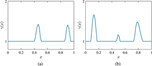This process begins by drawing an n-variate Gaussian vector as $\hat{\mathit{\alpha }}$, finding $\mathit{\alpha }$ and $\mathit{\theta }$ from (57(57) $\{\begin{array}{l}\mathit{\theta }=\rho (\mathit{\alpha })\\ \mathit{\alpha }=\mathbf{G}\hat{\mathit{\alpha }}\end{array}$(57) ), and constructing the field by using (34(34) ${\gamma }^h(x)=\mathit{\phi }(x{)}^{\mathrm{T}}\mathit{\theta }$(34) ). Some examples of such scalar fields are shown in Figures 2 and 3. The plots of these figures are generated by setting n = 64 and two different values of r. As seen the length and shape of the damage can be controlled by adjusting r.

5. Bayesian inversion of forward model

In this section, we apply the Bayesian inversion method described in [4] to solve the damage identification problem at hand. From the results of the previous sections, we can formulate the beam damage identification problem by using the following equations: (59) $\{\begin{array}{ll}\mathbf{d}=\mathbf{A}\mathit{\theta }+\mathbf{e}& (1)\\ \mathit{\theta }=\rho (\mathit{\alpha })& (2)\\ \lambda (x)={\displaystyle \frac{1}{\mathit{\phi }(x{)}^{\mathrm{T}}\mathit{\theta }}}& (3)\\ \mathit{\alpha }\sim \mathcal{N}(\mathbf{0},{\mathbf{\Gamma }}_{\alpha })& (4)\\ \mathbf{e}\sim \mathcal{N}({\mathit{\mu }}_e,{\mathbf{\Gamma }}_e)& (5)\end{array}$(59) The first equation, suggested by (42(42) $\mathbf{d}=\mathbf{A}\mathit{\theta }+\mathbf{e}$(42) ), represents the computational forward model of the problem. In this equation, $\mathbf{A}\in {\mathbb{R}}^{m\times n}$ is a constant matrix, data vector $\mathbf{d}\in {\mathbb{R}}^m$ which is the input variable obtained by direct measurement, $\mathit{\theta }\in {\mathbb{R}}^n$ is the unknown variable and $\mathbf{e}\in {\mathbb{R}}^m$ represents the measurement noise. The second equation, suggested by (57(57) $\{\begin{array}{l}\mathit{\theta }=\rho (\mathit{\alpha })\\ \mathit{\alpha }=\mathbf{G}\hat{\mathit{\alpha }}\end{array}$(57) ), models the mapping between $\mathit{\theta }\in {\mathbb{R}}^n$, and an n-variate Gaussian variable, $\mathit{\alpha }\in {\mathbb{R}}^n$. The third equation, suggested by (5(5) $\gamma (x)=\frac{1}{\lambda (x)}$(5) ) and (34(34) ${\gamma }^h(x)=\mathit{\phi }(x{)}^{\mathrm{T}}\mathit{\theta }$(34) ), relates the damage function (the primary unknown of the problem) to $\mathit{\theta }\in {\mathbb{R}}^n$. The fourth equation, suggested by (58(58) $\mathit{\alpha }\sim \mathcal{N}({\mathbf{0}}_n,\mathbf{G}{\mathbf{G}}^{\mathrm{T}})$(58) ), models $\mathit{\alpha }$ as an n-variate Gaussian variable whose mean vector and covariance matrix are $\mathbf{0}$ and ${\mathbf{\Gamma }}_{\alpha }$. This equation leads to (60) ${\pi }_{\alpha }(\mathit{\alpha })\propto \exp \{-\frac{1}{2}\Vert {\mathbf{L}}_{\alpha }\mathit{\alpha }{\Vert }^2\}$(60) where ${\mathbf{L}}_{\alpha }$ can be obtained by Cholesky decompositions of ${\mathbf{\Gamma }}_{\alpha }^{-1}$ as ${\mathbf{\Gamma }}_{\alpha }^{-1}={\mathbf{L}}_{\alpha }^{\mathrm{T}}{\mathbf{L}}_{\alpha }$. The fifth equation models the measurement noise vector as an m-variate Gaussian variable whose mean vector and covariance matrix are ${\mathit{\mu }}_e\in {\mathbb{R}}^m$ and ${\mathbf{\Gamma }}_e\in {\mathbb{R}}^{m\times m}$. This equation leads to (61) ${\pi }_e(\mathbf{e})\propto \exp \{-\frac{1}{2}\Vert {\mathbf{L}}_e(\mathbf{e}-{\mathit{\mu }}_e){\Vert }^2\}$(61) where ${\mathbf{L}}_e$ can be obtained by Cholesky decompositions of ${\mathbf{\Gamma }}_e^{-1}$ as ${\mathbf{\Gamma }}_e^{-1}={\mathbf{L}}_e^{\mathrm{T}}{\mathbf{L}}_e$. By using the analysis given in [46,49], we formulate the likelihood density function ${\pi }_{d|\alpha }(\mathbf{d}|\mathit{\alpha })$ (62) ${\pi }_{d|\alpha }(\mathbf{d}|\mathit{\alpha })\propto \exp (-\frac{1}{2}\Vert {\mathbf{L}}_e(\mathbf{d}-\mathbf{A}\rho (\mathit{\alpha })-{\mathit{\mu }}_e)\Vert {)}^2$(62) According to the Bayes' theorem, the posterior density ${\pi }_{\alpha |d}(\mathit{\alpha }|\mathbf{d})$ is related to the likelihood density function by (63) ${\pi }_{\alpha |d}(\mathit{\alpha }|\mathbf{d})\propto {\pi }_{\alpha }(\mathit{\alpha }){\pi }_{d|\alpha }(\mathbf{d}|\mathit{\alpha })$(63) By substituting (62(62) ${\pi }_{d|\alpha }(\mathbf{d}|\mathit{\alpha })\propto \exp (-\frac{1}{2}\Vert {\mathbf{L}}_e(\mathbf{d}-\mathbf{A}\rho (\mathit{\alpha })-{\mathit{\mu }}_e)\Vert {)}^2$(62) ) into (63(63) ${\pi }_{\alpha |d}(\mathit{\alpha }|\mathbf{d})\propto {\pi }_{\alpha }(\mathit{\alpha }){\pi }_{d|\alpha }(\mathbf{d}|\mathit{\alpha })$(63) ) and using (60(60) ${\pi }_{\alpha }(\mathit{\alpha })\propto \exp \{-\frac{1}{2}\Vert {\mathbf{L}}_{\alpha }\mathit{\alpha }{\Vert }^2\}$(60) ) we obtain (64) ${\pi }_{\alpha |d}(\mathit{\alpha }|\mathbf{d})\propto \exp (-\frac{1}{2}(\Vert {\mathbf{L}}_{\alpha }\mathit{\alpha }{\Vert }^2+\Vert {\mathbf{L}}_e(\mathbf{d}-\mathbf{A}\rho (\mathit{\alpha })-{\mathit{\mu }}_e){\Vert }^2))$(64) This equation can be re-arranged to obtain (65) ${\pi }_{\alpha |d}(\mathit{\alpha }|\mathbf{d})\propto \exp (-\frac{1}{2}\Vert \mathfrak{A}(\mathit{\alpha })-\mathit{b}{\Vert }^2)$(65) where vectors $\mathfrak{A}(\mathit{\alpha })$ and $\mathit{b}$ are given by (66) $\mathfrak{A}(\mathit{\alpha })=\left[\begin{array}{c}{\mathbf{L}}_{\alpha }\mathit{\alpha }\\ {\mathbf{L}}_e\mathbf{A}\rho (\mathit{\alpha })\end{array}\right]$(66) and (67) $\mathit{b}=\left[\begin{array}{c}{\mathbf{L}}_{\alpha }{\mathit{\mu }}_{\alpha }\\ {\mathbf{L}}_e(\mathbf{d}-{\mathit{\mu }}_e)\end{array}\right]$(67)

Figure 2. Random samples of γ generated by using the proposed method with n = 64 and r = 0.05.

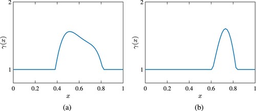
Figure 3. Random samples of γ generated by using the proposed method with n = 64 and r = 0.1.

5.1. Calculation of maximum A posteriori point estimate

The density function given in (65(65) ${\pi }_{\alpha |d}(\mathit{\alpha }|\mathbf{d})\propto \exp (-\frac{1}{2}\Vert \mathfrak{A}(\mathit{\alpha })-\mathit{b}{\Vert }^2)$(65) ) models the posterior density for $\mathit{\alpha }$. In this stage, we consider computing the Maximum a Posteriori point (MAP) estimate from this density function. By definition, the MAP estimate of $\mathit{\alpha }$ is obtained from the optimization problem of (68) ${\mathit{\alpha }}_{\mathrm{MAP}}=\arg \underset{\alpha }{max}{\pi }_{\alpha |d}(\mathit{\alpha }|\mathbf{d})$(68) Combining this equation and (65(65) ${\pi }_{\alpha |d}(\mathit{\alpha }|\mathbf{d})\propto \exp (-\frac{1}{2}\Vert \mathfrak{A}(\mathit{\alpha })-\mathit{b}{\Vert }^2)$(65) ) leads to (69) ${\mathit{\alpha }}_{\mathrm{MAP}}=\arg \underset{\alpha }{min}\Vert \mathfrak{A}(\mathit{\alpha })-\mathit{b}{\Vert }^2$(69) which is a non-linear optimization problem. Appendix 3 gives an iterative method based on line search method for computing ${\mathit{\alpha }}_{\mathrm{MAP}}$ from (70) ${\mathit{\alpha }}^{(l+1)}={\mathit{\alpha }}^{(l)}+k\mathbf{s}$(70) where k is the line search step-size. The above process can be repeated until the norm of $\mathbf{s}$ reaches a default value or some pre-defined conditions were met and (71) ${\mathit{\alpha }}^{(l)}\to {\mathit{\alpha }}_{\mathrm{MAP}}$(71) Recalling that $\mathit{\theta }=\rho (\mathit{\alpha })$ from (59.2), ${\mathit{\alpha }}_{\mathrm{MAP}}$ corresponds to a point estimate for $\mathit{\theta }$ given by (72) $\hat{\mathit{\theta }}=\rho ({\mathit{\alpha }}_{\mathrm{MAP}})$(72) Although ${\mathit{\alpha }}_{\mathrm{MAP}}$ is a maximum a posteriori estimation for $\mathit{\alpha }$, the value obtained for $\hat{\mathit{\theta }}$ by using the above equation is not necessary a maximum a posteriori estimation for $\mathit{\theta }$. Finally, from (59(59) $\{\begin{array}{ll}\mathbf{d}=\mathbf{A}\mathit{\theta }+\mathbf{e}& (1)\\ \mathit{\theta }=\rho (\mathit{\alpha })& (2)\\ \lambda (x)={\displaystyle \frac{1}{\mathit{\phi }(x{)}^{\mathrm{T}}\mathit{\theta }}}& (3)\\ \mathit{\alpha }\sim \mathcal{N}(\mathbf{0},{\mathbf{\Gamma }}_{\alpha })& (4)\\ \mathbf{e}\sim \mathcal{N}({\mathit{\mu }}_e,{\mathbf{\Gamma }}_e)& (5)\end{array}$(59) -3), the damage functions corresponding to $\hat{\mathit{\theta }}$ and ${\mathit{\alpha }}_{\mathrm{MAP}}$ can be computed by (73) $\hat{\lambda }(x)=\frac{1}{\mathit{\phi }(x{)}^{\mathrm{T}}\hat{\mathit{\theta }}}$(73) In the above analysis, we use the line-search algorithm to get numerical results because it is simple; however, other computationally efficient or low-cost algorithms may be used. The scope of the paper is not about such algorithms and their computational complexity or performance. As for a comparison against other methods, it is not relevant to compare the proposed method which provides posterior error estimates (in addition to the point estimates) to any method that does not provide such error estimates.

5.2. Quantification of uncertainty

To compute an estimate for the standard deviation of the posterior density function given in (65(65) ${\pi }_{\alpha |d}(\mathit{\alpha }|\mathbf{d})\propto \exp (-\frac{1}{2}\Vert \mathfrak{A}(\mathit{\alpha })-\mathit{b}{\Vert }^2)$(65) ), we approximate (65(65) ${\pi }_{\alpha |d}(\mathit{\alpha }|\mathbf{d})\propto \exp (-\frac{1}{2}\Vert \mathfrak{A}(\mathit{\alpha })-\mathit{b}{\Vert }^2)$(65) ) by a Gaussian density function. The exponent of (65(65) ${\pi }_{\alpha |d}(\mathit{\alpha }|\mathbf{d})\propto \exp (-\frac{1}{2}\Vert \mathfrak{A}(\mathit{\alpha })-\mathit{b}{\Vert }^2)$(65) ) includes $-\frac{1}{2}\mathfrak{F}(\alpha )$. In this case, we can use the Taylor series of $\mathfrak{F}(\alpha )$ to approximate (65(65) ${\pi }_{\alpha |d}(\mathit{\alpha }|\mathbf{d})\propto \exp (-\frac{1}{2}\Vert \mathfrak{A}(\mathit{\alpha })-\mathit{b}{\Vert }^2)$(65) ) by a Gaussian density. By using (A11(A11) $\mathfrak{F}(\mathit{\alpha })=\Vert \mathfrak{A}(\mathit{\alpha })-\mathit{b}{\Vert }^2$(A11) ), this series can be written in the form of: (74) $\mathfrak{F}(\mathit{\alpha })\approx ({\mathfrak{A}}_o-\mathfrak{b}{)}^{\mathrm{T}}({\mathfrak{A}}_o-\mathfrak{b})+2({\mathfrak{A}}_o-\mathfrak{b}{)}^{\mathrm{T}}{\mathfrak{J}}_o^{\mathrm{T}}(\mathit{\alpha }-{\mathit{\alpha }}_o)+(\mathit{\alpha }-{\mathit{\alpha }}_o{)}^{\mathrm{T}}({\mathfrak{J}}_o^{\mathrm{T}}{\mathfrak{J}}_o)(\mathit{\alpha }-{\mathit{\alpha }}_o)$(74) where ${\mathfrak{A}}_o$ and ${\mathfrak{J}}_o$ denote $\mathfrak{A}({\mathit{\alpha }}_o)$ and $\mathfrak{J}({\mathit{\alpha }}_o)$ respectively. This equation can be written in the standard quadratic form of (75) $\mathfrak{F}(\mathit{\alpha })\approx ({\mathfrak{A}}_o-\mathfrak{b}+{\mathfrak{J}}_o^{\mathrm{T}}(\mathit{\alpha }-{\mathit{\alpha }}_o){)}^{\mathrm{T}}({\mathfrak{A}}_o-\mathfrak{b}+{\mathfrak{J}}_o^{\mathrm{T}}(\mathit{\alpha }-{\mathit{\alpha }}_o))$(75) Recalling that $-\frac{1}{2}\mathfrak{F}(\alpha )$ is the exponent of the posterior density function ${\pi }_{\alpha |d}(\mathit{\alpha }|\mathbf{d})$; one can infer from (75(75) $\mathfrak{F}(\mathit{\alpha })\approx ({\mathfrak{A}}_o-\mathfrak{b}+{\mathfrak{J}}_o^{\mathrm{T}}(\mathit{\alpha }-{\mathit{\alpha }}_o){)}^{\mathrm{T}}({\mathfrak{A}}_o-\mathfrak{b}+{\mathfrak{J}}_o^{\mathrm{T}}(\mathit{\alpha }-{\mathit{\alpha }}_o))$(75) ) that the covariance matrix of the approximate Gaussian density is (76) ${\mathbf{\Gamma }}_{\alpha |d}\approx ({\mathfrak{J}}_o^{\mathrm{T}}{\mathfrak{J}}_o{)}^{-1}$(76) In this case, the diagonal elements of this covariance matrix, denoted by ${\sigma }_1^2,\dots ,{\sigma }_n^2$, represent the variances of the elements of $\mathit{\alpha }$; consequently, their square roots are equal to the standard deviations of the elements of $\mathit{\alpha }$. Therefore, we can compute the one-standard-deviation interval around the estimated value for $\mathit{\alpha }$. The upper and lower bounds of this interval by ${\mathit{\alpha }}_{\mathrm{MAP}}\pm \mathit{\sigma }$; where $\mathit{\sigma }=[{\sigma }_k{]}_{n\times 1}$ is the vector of standard deviations. Finally, the interval quantifying the uncertainty of the point estimate for the damage field can be computed from (59(59) $\{\begin{array}{ll}\mathbf{d}=\mathbf{A}\mathit{\theta }+\mathbf{e}& (1)\\ \mathit{\theta }=\rho (\mathit{\alpha })& (2)\\ \lambda (x)={\displaystyle \frac{1}{\mathit{\phi }(x{)}^{\mathrm{T}}\mathit{\theta }}}& (3)\\ \mathit{\alpha }\sim \mathcal{N}(\mathbf{0},{\mathbf{\Gamma }}_{\alpha })& (4)\\ \mathbf{e}\sim \mathcal{N}({\mathit{\mu }}_e,{\mathbf{\Gamma }}_e)& (5)\end{array}$(59) -3) by (77) $\{\begin{array}{l}{\lambda }_{\mathrm{U}}(x)={\displaystyle \frac{1}{\mathit{\phi }(x{)}^{\mathrm{T}}\rho ({\mathit{\alpha }}_{\mathrm{MAP}}+\mathit{\sigma })}}\\ {\lambda }_{\mathrm{L}}(x)={\displaystyle \frac{1}{\mathit{\phi }(x{)}^{\mathrm{T}}\rho ({\mathit{\alpha }}_{\mathrm{MAP}}-\mathit{\sigma })}}\end{array}$(77)

6. Numerical results

In this section, we assess the performance of the proposed damage identification method for both Euler-Bernoulli and Timoshenko beams. In the numerical experiments conducted in this section, we consider a beam with ${\beta }_0=5$ and an external force $f(x)$ given by (78) $f(x)=\{\begin{array}{ll}-1& 0.3<x<0.7\\ 0& \mathrm{else}\end{array}$(78) The beam is damaged such that $\lambda (x)$ has a linear drop in the interval of $[0.2,0.3]$ and a linear rise in the interval of $[0.3,0.4]$. In other words, the beam suffers a local damage around x = 0.3. We compute the static response of the undamaged beam by setting $\lambda (x)=1$ in the proposed forward model. Also, we compute the static response of the damaged beam by using the assumed $\lambda (x)$ in the proposed forward model. We use the latter response to generate the data vector in the following experiments.

6.1. Experiment 1

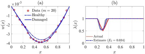
In the first experiment, we consider an Euler-Bernoulli model for the beam. We suppose that the dimensions of the data vector (m = 20) is smaller than that of the unknown vector (n = 40), and the data Signal-to-Noise-Ratio (SNR) is low. To this end, we perform the following tasks:

1. We collect the values of the response at m = 20 equally spaced points and add Gaussian white noise to them such that the data SNR is only $20\mathrm{dB}$. The data points are shown in Figure 4(a). Also, full static responses of the beam in healthy and damaged conditions are shown in this figure.

2. We form a data vector by using the collected data points and feed it to the proposed identification method to compute the estimate of $\lambda (x)$ shown by $\hat{\lambda }(x)$. The result is demonstrated in Figure 4(b). The effectiveness of the proposed identification method can be verified visually in Figure 4(b). Additionally, we compute the identification error as $E_{\delta }=\Vert {\mathit{\alpha }}_{\mathrm{MAP}}-\mathit{\alpha }\Vert =0.037$. By using (77(77) $\{\begin{array}{l}{\lambda }_{\mathrm{U}}(x)={\displaystyle \frac{1}{\mathit{\phi }(x{)}^{\mathrm{T}}\rho ({\mathit{\alpha }}_{\mathrm{MAP}}+\mathit{\sigma })}}\\ {\lambda }_{\mathrm{L}}(x)={\displaystyle \frac{1}{\mathit{\phi }(x{)}^{\mathrm{T}}\rho ({\mathit{\alpha }}_{\mathrm{MAP}}-\mathit{\sigma })}}\end{array}$(77) ), we compute the range of $\lambda (x)$ within one standard deviation of the MAP estimate and show it by using gray shading in Figure 4(b). In other words, the gray area indicates the uncertainty of the estimated solution. The results demonstrated above is indicating an insight to the spatial distribution of $\lambda (x)$ given the existing constraints in the data size and SNR. As seen in Figure 4, the actual values of $\lambda (x)$ are almost within the one-standard-deviation interval of the computed point estimate; however, there are some errors due to neglecting approximation error. Potentially, the errors can be reduced by using Bayesian Approximation Error approach [4], leading to a future investigation for the current work.

3. We can also compute the marginal prior and posterior densities of elements of $\alpha \in {\mathbb{R}}^{40}$. For example, we consider the 12th and 14th elements of α and plot their marginal densities in Figure 5. In this figure, the prior and posterior densities are shown. Also the corresponding actual values are shown. As seen, the prior densities of both ${\alpha }_{12}$ and ${\alpha }_{14}$ are very flat (indicating high uncertainty); however, their posterior densities are much sharper and their peak values are very close to the actual values. This behaviour verifies that the proposed method decreases the uncertainty of the initial guess (prior data).

4. By using the probabilistic model we found for α, we can compute a probabilistic model for $\lambda (x)$ from $\lambda (x)=\frac{1}{\mathit{\phi }(x{)}^{\mathrm{T}}\rho (\mathit{\alpha })}$ and evaluate its values at some points on the beam. We can then numerically calculate the co-variance matrix for all the computed values for $\lambda (x)$. For example, Figure 6 visualize the co-variance matrix of $\lambda (x)$ values computed for 2000 equally spaced locations on the beam which indicates no cross-talk between the damaged and undamaged regions.

5. We can also compute a histogram for every value of $\lambda (x)$. Figure 7(a) shows the histograms for $\lambda (x)$ at x = 0.25 which is a damaged location. Figure 7(b) shows the histograms for $\lambda (x)$ at x = 0.8 which is an undamaged location. As seen the histogram shows that the probability density of $\lambda (x)$ is concentrated at 1.

Figure 4. Damage identification of a simply-supported Euler-Bernoulli beam by using proposed method (a): beam responses and data points, (b): identification result.

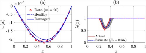
Figure 5. Prior and posterior marginal densities of two ${\alpha }_{12}$ and ${\alpha }_{14}$ in experiment 1.

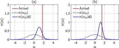
Figure 6. Visualization of the co-variance matrix of the estimated values of $\lambda (x)$ at 2000 equally-spaced locations – Experiment 1.

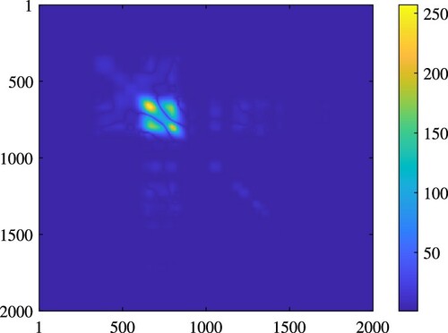
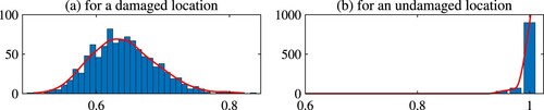
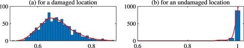
Figure 7. Histograms of the estimated values of $\lambda (x)$ at a damaged location (x = 0.25) and an undamaged location ($x=0.9)$ – Experiment 1.

6.2. Experiment 2

In the second experiment, we consider a Timoshenko model for the beam with $k_0=0.01$; we use the same ${\beta }_0$, $\lambda (x)$ and $f(x)$ used in the previous experiment. We compute the static responses of the healthy and damaged beams and generate the data vector as discussed in the previous example. Again, we aim at testing the proposed method when the dimensions of the data vector (m = 20) is smaller than that of the unknown vectors (n = 40), and the data SNR is low. We perform the two first tasks introduced for the first experiment. As the result of the first task, the data points are shown in Figure 8(a). As the result of the second task, ${\lambda }_{\mathrm{SOL}}(x)$ is shown in Figure 8(b). The identification error is about $E_{\delta }=0.034$ for this experiment. Again, the results of the above experiment indicate that the actual values of $\lambda (x)$ are almost within the one-standard-deviation interval of the computed point estimate. The existing errors are made due to neglecting approximation errors as mentioned in the first experiment.

Figure 8. Damage identification of a simply-supported Timoshenko beam by using proposed method (a): beam responses and data points, (b): identification result.

We also repeat the fourth and fifth tasks to visualize the co-variance matrix of the evaluated values of the damage function $\lambda (x)$, as shown in Figures 9 and sample histograms for a damaged point at x = 0.25, shown in Figure 10(a), and an undamaged point at x = 0.9, shown in Figure 10(b).

Figure 9. Visualization of the co-variance matrix of the estimated values of $\lambda (x)$ at 2000 equally-spaced points – Experiment 2.

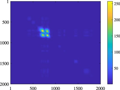
Figure 10. Histograms of the estimated values of $\lambda (x)$ at a damaged location (x = 0.25) and an undamaged location ($x=0.9)$ – Experiment 2.

6.3. Experiment 3

In the third experiment, we repeat the first experiment with a damage function modeling two damage areas across the beam. We compute the static responses of the healthy and damaged beams and generate the data vector as discussed in the previous example. We aim at testing the proposed method when the dimensions of the data vector (m = 40) is smaller than that of the unknown vectors (n = 80), and the data SNR is low. We perform the two first tasks introduced for the first experiment. As the result of the first task, the data points are shown in Figure 11(a). As the result of the second task, the estimated value of $\lambda (x)$ is shown in Figure 11(b). The identification error is about $E_{\delta }=0.07$ for this experiment. Again, the results of the above experiment indicate that the actual values of $\lambda (x)$ are almost within the one-standard-deviation interval of the computed point estimate. The existing errors are made due to neglecting approximation errors as mentioned in the previous experiments. We also carry ut the forth step and compute the co-variance matrix of $\lambda (x)$, which indicates positive cross-talk between the damaged areas. Finally we carry out the fifth step for this experiment and compute two sample histograms, one for a damaged location and one for an undamaged location. The results are shown in Figures 12 and 13. 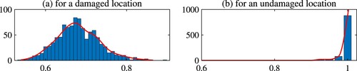Similar to the previous experiment, for a damaged location, the values of $\lambda (x)$ are distributed around the actual value. However, for an undamaged location, the values are concentrated at 1. This observation is consistent in all the experiments demonstrated above.

Figure 11. Damage identification of a simply-supported Euler-Bernoulli beam by using proposed method with two damaged area across the beam (a): beam responses and data points, (b): identification result.

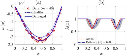
Figure 12. Visualization of the co-variance matrix of the estimated values of $\lambda (x)$ at 2000 equally-spaced locations – Experiment 3.

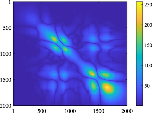
Figure 13. Histograms of the estimated values of $\lambda (x)$ at a damaged location (x = 0.25) and an undamaged location ($x=0.6)$ – Experiment 2.

7. Conclusion

The damage identification of a simply-supported beam when the distributed external force applied to the beam is static and the observed data includes noisy and limited data on static beam response has been a challenge. In the theory of elasticity, the static response of a damaged simply-supported beam is modeled by using an ordinary differential equation of order four with in-homogeneous coefficient functions. This equation can be split into two simple differential equations of order two with homogeneous coefficient functions. A forward computational model for the damage identification of the beam can be derived by applying the Galerkin Finite Element Method to these second-order equations. From a prior model for the damage field and some data on the static response of the beam, a posterior model for the damage field can be obtained. This model can be used to find a maximum a posteriori point estimate for the damage field and quantify the uncertainty associated with such an estimate. The results obtained from the experiments demonstrated in this paper indicates that the proposed damage identification method can estimate the damage field for both Euler-Bernoulli and Timoshenko beams even if the available data on the static beam response is limited and noisy. When the data is limited (or missing), the Bayesian framework can still identify the damage occurred across the beam. Moreover, it can estimate the error associated with the result. In this case, the accuracy of the proposed method might decrease; however, this method can estimate the errors (posterior standard deviations) of the result: naturally, in locations where there are few or no measurements, the posterior error stimates are large. In the conducted numerical experiments, the estimated damage field lies approximately within the interval corresponding to the one-standard-deviation interval. No cross-talk between the damaged and undamaged locations are observed; however, when there are two damaged location, a positive cross-talk between the damaged areas can be observed. This promising result can be seen for both Euler-Bernoulli and Timoshenko beams. The existing errors are due to neglecting approximation errors. Since the proposed methodology is only applied to numerical simulation, its practical application can be investigated by field measurement.

Disclosure statement

No potential conflict of interest was reported by the author(s).

Appendices

Appendix 1.

Computation of $\mathbf{\Phi }$, $\mathbf{B}$ and $\mathbf{H}$

The first step is to choose a basis for ${\mathcal{V}}^h(\mathrm{\Omega })$. Here, we form ${\mathcal{V}}^h(\mathrm{\Omega })$ by using the piece-wise linear basis functions (hat functions). We can formulate a typical basis function ${\phi }_i(x)$ by (A1) ${\phi }_i(x)=\{\begin{array}{ll}{\displaystyle \frac{1}{h}}x-i+2& max(0,ih-2h)\le x<ih-h\\ -{\displaystyle \frac{1}{h}}x+i& (i-1)h<x\le min(ih,1)\\ 0& else\end{array}$(A1) where $i\in \{1,\dots ,n\}$ and h is given by (A2) $h=\frac{1}{n-1}$(A2) The second step is to form $\mathit{\phi }(x)$ and $\mathbf{\Phi }$ by substituting (A1(A1) ${\phi }_i(x)=\{\begin{array}{ll}{\displaystyle \frac{1}{h}}x-i+2& max(0,ih-2h)\le x<ih-h\\ -{\displaystyle \frac{1}{h}}x+i& (i-1)h<x\le min(ih,1)\\ 0& else\end{array}$(A1) ) into (21(21) $\begin{array}{r}\mathit{\phi }(x)=[\begin{array}{ccc}{\phi }_1(x)& \dots & {\phi }_n(x)\end{array}{]}^{\mathrm{T}}\end{array}$(21) ) and (41(41) $\mathbf{\Phi }=[{\phi }_j({\xi }_i){]}_{m\times n}$(41) ). The third step starts with computing $\mathbf{B}$ and $\mathbf{a}$. By using (25(25) $\mathbf{B}=-{\beta }_0{\int }_{\mathrm{\Omega }}(\frac{\mathrm{d}}{\mathrm{d}x}\mathit{\phi }(x)){(\frac{\mathrm{d}}{\mathrm{d}x}\mathit{\phi }(x))}^{\mathrm{T}}\mathrm{d}x$(25) ) and using analytical integration methods, we can find $\mathbf{B}$ as (A3) $\mathbf{B}=\frac{1}{h}\left[\begin{array}{ccccccc}1& -1& 0& \cdots & & \cdots & 0\\ -1& 2& -1& \ddots & & & ⋮\\ 0& -1& 2& \ddots & \ddots \\ ⋮& \ddots & \ddots & \ddots & \ddots & \ddots & ⋮\\ & & \ddots & \ddots & 2& -1& 0\\ ⋮& & & \ddots & -1& 2& -1\\ 0& \cdots & & \cdots & 0& -1& 1\end{array}\right]$(A3) Unlike matrix $\mathbf{B}$, vector $\mathbf{a}$ is often computed numerically. This step is followed by forming the linear system of (24(24) $\mathbf{B}\mathbf{c}=\mathbf{a}$(24) ). The first and last equations of this system should be removed as the basis functions ${\phi }_1(x)$ and ${\phi }_n(x)$ do not satisfy the Dirichlet boundary condition. We can replace these two equations with the equations derived from the given boundary conditions. By substituting x = 0 into (20(20) $u^h(x)=\sum _{i=1}^n{c}_i{\phi }_i(x)=\mathit{\phi }(x{)}^{\mathrm{T}}\mathbf{c}$(20) ) and considering $u(0)=0$, we obtain (A4) $u(0)=\sum _{i=1}^n{c}_i{\phi }_i(0)=0\Rightarrow c_1=0$(A4) We now replace the first equation of $\mathbf{B}\mathbf{c}=\mathbf{a}$ with $c_1=0$. Similarly, by substituting x = 1 into (20(20) $u^h(x)=\sum _{i=1}^n{c}_i{\phi }_i(x)=\mathit{\phi }(x{)}^{\mathrm{T}}\mathbf{c}$(20) ) and considering $u(1)=0$, we obtain an equation in the form of (A5) $u(1)=\sum _{i=1}^n{c}_i{\phi }_i(1)=0\Rightarrow c_n=0$(A5) which can be used instead of the nth equation of the linear system. Finally, we find the coefficient vector $\mathbf{c}$ from the modified matrix equation in this step. The fourth step is to compute $\mathbf{H}$ by substituting the obtained value for $\mathbf{c}$ into (38(38) $\mathbf{H}={\int }_{\mathrm{\Omega }}({\mathbf{c}}^{\mathrm{T}}\mathit{\phi }({\mathit{\phi }\mathit{\phi }}^{\mathrm{T}})-k_{0}f{\mathit{\phi }\mathit{\phi }}^{\mathrm{T}}-{\beta }_0{k}_0{\mathbf{c}}^{\mathrm{T}}\frac{\mathrm{d}}{\mathrm{d}x}\mathit{\phi }\left(\mathit{\phi }\frac{\mathrm{d}}{\mathrm{d}x}{\mathit{\phi }}^{\mathrm{T}}\right))\mathrm{d}x$(38) ) and using numerical integration methods. Finally, having $\mathbf{\Phi }$, $\mathbf{B}$ and $\mathbf{H}$ we can compute $\mathbf{A}=\mathbf{\Phi }{\mathbf{B}}^{-1}\mathbf{H}$ and construct the computational forward model.

Appendix 2.

Modeling $\mathit{\alpha }$

The aim of this section is to compute $\mathit{\alpha }$ from $\hat{\mathit{\alpha }}$. To this end, we use a low-pass filter to construct the desired low-frequency field from the Gaussian field $\hat{\gamma }(x)$. This filtering process is formulated by (A6) $\mathbf{y}=\mathbf{g}⊛\hat{\mathbf{y}}$(A6) where vector $\mathbf{g}\in {\mathbb{R}}^n$ models the impulse response of a low-pass filter. Combining (48(48) $\hat{\mathbf{y}}=\hat{\mathit{\alpha }}$(48) ), (50(50) $\mathbf{y}=\mathit{\alpha }$(50) ) and (A6(A6) $\mathbf{y}=\mathbf{g}⊛\hat{\mathbf{y}}$(A6) ) results in (A7) $\mathit{\alpha }=\mathbf{g}⊛\hat{\mathit{\alpha }}$(A7) This result is valid only when piece-wise linear functions given by (A1(A1) ${\phi }_i(x)=\{\begin{array}{ll}{\displaystyle \frac{1}{h}}x-i+2& max(0,ih-2h)\le x<ih-h\\ -{\displaystyle \frac{1}{h}}x+i& (i-1)h<x\le min(ih,1)\\ 0& else\end{array}$(A1) ) are used for modeling scalar fields. By using the properties of the cyclic convolution[66], we can re-write (A7(A7) $\mathit{\alpha }=\mathbf{g}⊛\hat{\mathit{\alpha }}$(A7) ) as (A8) $\mathit{\alpha }=\mathbf{G}\hat{\mathit{\alpha }}$(A8) where $\mathbf{G}\in {\mathbb{R}}^{n\times n}$ is defined by (A9) $G_{i,j}=\{\begin{array}{ll}{g}_{i-j+1}& 1<j\le i\\ g_{n+i-j+1}& i<j\le n\end{array}$(A9) As seen, the jth column of $\mathbf{G}$ can be obtained by circular shift of vector $\mathbf{g}$ by j−1 position. Noting that $\hat{\mathit{\alpha }}$ is a known vector from the beginning of the analysis, we just need to find an appropriate realization for the low-pass filter so that we can compute $\mathit{\alpha }$ and $\gamma (x)$ by using (A8(A8) $\mathit{\alpha }=\mathbf{G}\hat{\mathit{\alpha }}$(A8) ) and (45(45) ${\hat{\gamma }}^h(x)=\sum _{i=1}^n{\hat{\alpha }}_i{\phi }_i(x)=\mathit{\phi }(x{)}^{\mathrm{T}}\hat{\mathit{\alpha }}$(45) ). Several methods for designing discrete filters, also known as digital filters, have been proposed in the theory of digital signal processing. The design of such filters is not within the scope of this paper. The readers may refer to [67] and [68] for more detail about digital filters. In the following, we only consider Hamming low-pass filters. The detailed derivation of this filter can be found in [68]. For a Hamming low-pass filter, we have: (A10) $g_i=\frac{1}{\Vert \mathbf{g}\Vert }(0.54-0.46\cos \frac{2\pi (i-1)}{n-1})\mathrm{sinc}(\pi r(2i-n-1))$(A10) where $i\in \{1,\dots ,n\}$ and 0<r<1 is the normalized cut-off frequency.

Appendix 3.

Estimation of search direction

Here, we use the Gauss-Newton method to solve the problem at hand. To this end, we form the functional (A11) $\mathfrak{F}(\mathit{\alpha })=\Vert \mathfrak{A}(\mathit{\alpha })-\mathit{b}{\Vert }^2$(A11) and construct its Taylor series as (A12) $\mathfrak{F}({\mathit{\alpha }}_o+\mathbf{s})=\mathfrak{F}({\mathit{\alpha }}_o)+\{\mathrm{\nabla }\mathfrak{F}({\mathit{\alpha }}_o){\}}^{\mathrm{T}}\mathbf{s}+\frac{1}{2}{\mathbf{s}}^{\mathrm{T}}\{\mathrm{\nabla }\mathrm{\nabla }\mathfrak{F}({\mathit{\alpha }}_o)\}\mathbf{s}+\mathcal{O}(\Vert \mathbf{s}{\Vert }^3)$(A12) where ${\mathit{\alpha }}_o\in {\mathbb{R}}^n$ is an initial guess for $\mathit{\alpha }$ and $\mathbf{s}\in {\mathbb{R}}^n$ is the search direction. To find $\mathbf{s}$ we can use the line search method [69] and minimize $\mathfrak{F}({\mathit{\alpha }}_o+\mathbf{s})$ by setting $\mathrm{\nabla }\mathfrak{F}({\mathit{\alpha }}_o+\mathbf{s})$ to zero and neglecting $\mathcal{O}(\Vert \mathbf{s}{\Vert }^3)$, resulting in (A13) $\mathbf{s}=-\{\mathrm{\nabla }\mathrm{\nabla }\mathfrak{F}({\mathit{\alpha }}_o){\}}^{-1}\mathrm{\nabla }\mathfrak{F}({\mathit{\alpha }}_o)$(A13) From the definition of the Jacobian matrix [69], $\mathrm{\nabla }\mathfrak{F}({\mathit{\alpha }}_o)$ can be calculated by (A14) $\mathrm{\nabla }\mathfrak{F}({\mathit{\alpha }}_o)=\mathfrak{J}({\mathit{\alpha }}_o)(\mathfrak{A}({\mathit{\alpha }}_o)-\mathfrak{b})$(A14) where $\mathfrak{J}\mathbf{(}\mathit{\alpha }\mathbf{)}$ denotes the Jacobian of $\mathfrak{A}(\mathit{\alpha })$. From Gauss-Newton approximation [69], (A15) $\mathrm{\nabla }\mathrm{\nabla }\mathfrak{F}({\mathit{\alpha }}_o)=\mathfrak{J}({\mathit{\alpha }}_o){}^{\mathrm{T}}\mathfrak{J}({\mathit{\alpha }}_o)$(A15) After substituting (A14(A14) $\mathrm{\nabla }\mathfrak{F}({\mathit{\alpha }}_o)=\mathfrak{J}({\mathit{\alpha }}_o)(\mathfrak{A}({\mathit{\alpha }}_o)-\mathfrak{b})$(A14) ) and (A15(A15) $\mathrm{\nabla }\mathrm{\nabla }\mathfrak{F}({\mathit{\alpha }}_o)=\mathfrak{J}({\mathit{\alpha }}_o){}^{\mathrm{T}}\mathfrak{J}({\mathit{\alpha }}_o)$(A15) ) into (A13(A13) $\mathbf{s}=-\{\mathrm{\nabla }\mathrm{\nabla }\mathfrak{F}({\mathit{\alpha }}_o){\}}^{-1}\mathrm{\nabla }\mathfrak{F}({\mathit{\alpha }}_o)$(A13) ), we have: (A16) $\mathbf{s}=-\{\mathfrak{J}({\mathit{\alpha }}_o){}^{\mathrm{T}}\mathfrak{J}({\mathit{\alpha }}_o){\}}^{-1}\mathfrak{J}({\mathit{\alpha }}_o)(\mathfrak{A}({\mathit{\alpha }}_o)-\mathit{b})$(A16) More detail on the line search method described above can be found in the third chapter of [69]. The next step is to find the Jacobian of $\mathfrak{A}$. Recalling that for the chosen function ρ the ith element of $\rho (\alpha )$ depends on only the ith element of $\mathit{\alpha }$, we can compute the Jacobian of $\mathfrak{A}$ from (A13(A13) $\mathbf{s}=-\{\mathrm{\nabla }\mathrm{\nabla }\mathfrak{F}({\mathit{\alpha }}_o){\}}^{-1}\mathrm{\nabla }\mathfrak{F}({\mathit{\alpha }}_o)$(A13) ) as: (A17) $\mathfrak{J}(\mathit{\alpha })={\left[\begin{array}{c}{\mathbf{L}}_e\mathbf{A}\mathbf{\Lambda }\\ {\mathbf{L}}_{\alpha }\end{array}\right]}_{(m+n)\times n}$(A17) where (A18) $\mathbf{\Lambda }=\mathrm{diag}(\frac{\mathrm{d}\rho }{\mathrm{d}t}({\alpha }_1),\dots ,\frac{\mathrm{d}\rho }{\mathrm{d}t}({\alpha }_n))$(A18) Now, by substituting $\mathfrak{J}(\mathit{\alpha })$ into (A16(A16) $\mathbf{s}=-\{\mathfrak{J}({\mathit{\alpha }}_o){}^{\mathrm{T}}\mathfrak{J}({\mathit{\alpha }}_o){\}}^{-1}\mathfrak{J}({\mathit{\alpha }}_o)(\mathfrak{A}({\mathit{\alpha }}_o)-\mathit{b})$(A16) ) we can find $\mathbf{s}$.

References

- Sokolnikoff I. Mathematical theory of elasticity. New York, NY: McGraw-Hill; 1956.
- Eskin G, Ralston J. On the inverse boundary value problem for linear isotropic elasticity. Inverse Probl. 2002 May;18:907–921.
- Bonnet M, Constantinescu A. Inverse problems in elasticity. Inverse Probl. 2005 Feb;21:R1–R50.
- Kaipio J, Somersalo E. Statistical and computational inverse problems. 1st ed. New York: Springer-Verlag; 2005.
- Busby H, Trujillo D. Optimal regularization of an inverse dynamics problem. Comput Struct. 1997;63(2):243–248.
- Hollandsworth P, Busby H. Impact force identification using the general inverse technique. Int J Impact Eng. 1989;8(4):315–322.
- Adams R, Doyle JF. Multiple force identification for complex structures. Exp Mech. 2002 Mar;42:25–36.
- Karlsson SES. Identification of external structural loads frommeasured harmonic responses. J Sound Vib. 1996;196(1):59–74.
- Jacquelin E, Bennani A, Hamelin P. Force reconstruction: analysis and regularization of a deconvolution problem. J Sound Vib. 2003;265(1):81–107.
- Aucejo M. Structural source identification using a generalized Tikhonov regularization. J Sound Vib. 2014;333(22):5693–5707.
- Aucejo M, Smet OD. Bayesian source identification using local priors. Mech Syst Signal Process. 2016;66–67:120–136.
- Aucejo M, Smet OD. On a full Bayesian inference for force reconstruction problems. Mech Syst Signal Process. 2018;104:36–59.
- Sanchez J, Benaroya H. Review of force reconstruction techniques. J Sound Vib. 2014;333(14):2999–3018.
- Nakamura G, Uhlmann G. Inverse problems at the boundary for an elastic medium. SIAM J Math Anal. 1995;26(2):263–279.
- Lesnic D, Elliott L, Ingham D. Analysis of coefficient identification problems associated to the inverse Euler-Bernoulli beam theory. IMA J Appl Math. 1999;62(2):101–116.
- Lesnic D. Determination of the flexural rigidity of a beam from limited boundary measurements. J Appl Math Comput. 2006;20(1-2):17–34.
- Marinov TT, Marinova RS, Christov CI. Coefficient identification in elliptic partial differential equation. In: Lirkov I, Margenov S, Waśniewski J, editors. Large-scale scientific computing. Berlin Heidelberg: Springer; 2006. p. 372–379.
- Marinov TT, Vatsala AS. Inverse problem for coefficient identification in the Euler-Bernoulli equation. Comput Math Appl. 2008;56(2):400–410.
- Marinov TT, Marinova R. Inverse problem for coefficient identification in Euler-Bernoulli equation by linear spline approximation. In: Lirkov I, Margenov S, Waśniewski J, editors. Large-scale scientific computing. Berlin Heidelberg: Springer; 2010. p. 588–595.
- Marinov TT, Marinova RS. An inverse problem for estimation of bending stiffness in Kirchhoff-Love plates. Comput Math Appl. 2013;65(3):512–519. Efficient Numerical Methods for Scientific Applications.
- Dobson BJ, Rider E. A review of the indirect calculation of excitation forces from measured structural response data. Proc Inst Mech Eng C: Mech Eng Sci. 1990;204(2):69–75.
- Valentinuzzi ME, Montaldo Volachec EM. Discrete deconvolution. Med Biol Eng. 1975 Jan;13:123–125.
- Riad SM. The deconvolution problem: an overview. Proc IEEE. 1986 Jan;74:82–85.
- Karve PM, Na S-W, Kang JW, Kallivokas LF. The inverse medium problem for Timoshenko beams and frames: damage detection and profile reconstruction in the time-domain. Comput Mech. 2011 Feb;47:117–136.
- Castello DA, Kaipio JP. Modeling errors due to Timoshenko approximation in damage identification. Int J Numer Methods Eng. 2019;120(9):1148–1162.
- Morassi A, Rollo M. Identification of two cracks in a simply supported beam from minimal frequency measurements. J Vib Control. 2001;7(5):729–739.
- Ng C-T. On the selection of advanced signal processing techniques for guided wave damage identification using a statistical approach. Eng Struct. 2014;67:50–60.
- Guo J, Wang L, Takewaki I. Static damage identification in beams by minimum constitutive relation error. Inverse Probl Sci Eng. 2019;27(10):1347–1371.
- Ghrib F, Li L, Wilbur P. Damage identification of Euler-Bernoulli beams using static responces. J Eng Mech. 2012;138(5):405–415.
- Friswell MI. Damage identification using inverse methods. Phil Trans R Soc A: Math Phys Eng Sci. 2007;365(1851):393–410.
- Salawu O. Detection of structural damage through changes in frequency: a review. Eng Struct. 1997;19(9):718–723.
- Rucevskis S, Sumbatyan MA, Akishin P, Chate A. Tikhonov's regularization approach in mode shape curvature analysis applied to damage detection. Mech Res Commun. 2015;65:9–16.
- Fan W, Qiao P. Vibration-based damage identification methods: a review and comparative study. Struct Health Monitor. 2011;10(1):83–111.
- Gladwell GML, Bishop RED. The inverse problem for the vibrating beam. Proc R Soc Lond. A. Math Phys Sci. 1984;393(1805):277–295.
- Gladwell G. Inverse problems in vibration. 2nd ed. New York, NY: Springer; 2005.
- Tan G, Shan J, Wu C, Wang W. Direct and inverse problems on free vibration of cracked multiple I-section beam with different boundary conditions. Adv Mech Eng. 2017;9(11):1687814017737261.
- Zheng D, Kessissoglou N. Free vibration analysis of a cracked beam by finite element method. J Sound Vib. 2004;273(3):457–475.
- Busby HR, Trujillo DM. Solution of an inverse dynamics problem using an eigenvalue reduction technique. Comput Struct. 1987;25(1):109–117.
- Narkis Y. Identification of crack location in vibrating simply supported beams. J Sound Vib. 1994;172(4):549–558.
- Betti R. Time-domain identification of structural systems from input-output measurements. Vienna: Springer; 2008.67–93.
- Sellier M. An iterative method for the inverse elasto-static problem. J Fluids Struct. 2011;27(8):1461–1470.
- Viola E, Bocchini P. Non-destructive parametric system identification and damage detection in truss structures by static tests. Struct Infrastruct Eng. 2013;9(5):384–402.
- Banan MR, Banan MR, Hjelmstad KD. Parameter estimation of structures from static response. I. Computational aspects. J Struct Eng. 1994;120(11):3243–3258.
- Banan MR, Banan MR, Hjelmstad KD. Parameter estimation of structures from static response. II: Numerical simulation studies. J Struct Eng. 1994;120(11):3259–3283.
- Wang X, Hu N, Fukunaga H, Yao Z. Structural damage identification using static test data and changes in frequencies. Eng Struct. 2001;23(6):610–621.
- Ardekani I. Bayesian damage identification from elastostatic data [PhD thesis]. The University of Auckland; 2020.
- Tikhonov AN, Arsenin VY. Solutions of ill-posed problems. New York: Winston Wiley; 1977.
- Hansen PC. The truncated SVD as a method for regularization. BIT Numer Math. 1987 Dec;27:534–553.
- Kaipio J, Somersalo E. Statistical inverse problems: discretization, model reduction and inverse crimes. J Comput Appl Math. 2007;198(2):493–504. Special Issue: Applied Computational Inverse Problems.
- Kaipio J, Kolehmainen V. Approximate marginalization over modelling errors and uncertainties in inverse problems. In: Bayesian theory and applications. Oxford University Press; 2015.
- Smith CR, Bowers LK, Vogel RC. Numerical recovery of material parameters in Euler-Bernoulli beam models. J Math Syst Estim Control. 1991 Mar;7:359–373.
- Ng C-T. Bayesian model updating approach for experimental identification of damage in beams using guided waves. Struct Health Monitor. 2014;13(4):359–373.
- Khiem NT, Huyen NN. A method for crack identification in functionally graded Timoshenko beam. Nondestruct Test Eval. 2017;32(3):319–341.
- Chouiyakh H, Azrar L, Alnefaie K, Akourri O. Vibration and multi-crack identification of Timoshenko beams under moving mass using the differential quadrature method. Int J Mech Sci. 2017;120:1–11.
- Khatir S, Dekemele K, Loccufier M, Khatir T, Wahab MA. Crack identification method in beam-like structures using changes in experimentally measured frequencies and particle swarm optimization. CR Mecanique. 2018;346(2):110–120.
- He S, Ng C-T. Guided wave-based identification of multiple cracks in beams using a Bayesian approach. Mech Syst Signal Process. 2017;84:324–345.
- Teixeira JS, Stutz LT, Knupp DC, Silva-Neto AJ. Structural damage identification via time domain response and Markov Chain Monte Carlo method. Inverse Probl Sci Eng. 2017;25(6):909–935.
- Felippa C. A historical outline of matrix structural analysis: a play in three acts. Comput Struct. 2001;79(14):1313–1324.
- Castello D, Stutz L, Rochinha F. A structural defect identification approach based on a continuum damage model. Comput Struct. 2002;80(5):417–436.
- Da Costa Mattos H, Sampaio R. Analysis of the fracture of brittle elastic materials using a continuum damage model. Struct Eng Mech. 1995 Sep;3:411–428.
- Pires-Domingues S, Costa-Mattos H, Rochinha F. Modelling of nonlinear damage on elastic brittle materials. Mech Res Commun. 1998;25(2):147–153.
- Ciarlet PG. Finite element method for elliptic problems. Philadelphia, PA: Society for Industrial and Applied Mathematics; 2002.
- Ghannadi P, Kourehli S. Investigation of the accuracy of different finite element model reduction techniques. Struct Monit Maint. 2018 Sep;5:417–428.
- Stuart AM. Inverse problems: a Bayesian perspective. Acta Numer. 2010;19:451–559.
- Roininen L, Huttunen JMJ, Lasanen S. Whittle-Matérn priors for Bayesian statistical inversion with applications in electrical impedance tomography. Inverse Probl Imaging. 2014;8(2):561–586.
- Katznelson Y. An introduction to harmonic analysis; 1976.
- Haykin S. Adaptive filter theory. 4th ed. Upper Saddle River, NJ: Prentice Hall; 2002.
- Tan L, Jiang J. Finite impulse response filter design. In: Tan L, Jiang J, editors. Digital signal processing. 2nd ed. Boston: Academic Press; 2013. p. 217–299.
- Nocedal J, Wright S. Numerical optimization. New York: Springer; 2000. (Springer series in operations research and financial engineering).
Appendices
Appendix 1.
Computation of , and
The first step is to choose a basis for . Here, we form
by using the piece-wise linear basis functions (hat functions). We can formulate a typical basis function
by
(A1)
where
and h is given by
(A2)
The second step is to form
and
by substituting (EquationA1
(A1) ) into (Equation21
(21)
(21) ) and (Equation41
(41)
(41) ). The third step starts with computing
. By using (Equation25
(25)
(25) ) and using analytical integration methods, we can find
as
(A3)
Unlike matrix
, vector
is often computed numerically. This step is followed by forming the linear system of (Equation24
(24)
(24) ). The first and last equations of this system should be removed as the basis functions
do not satisfy the Dirichlet boundary condition. We can replace these two equations with the equations derived from the given boundary conditions. By substituting x = 0 into (Equation20
(20)
(20) ) and considering
, we obtain
(A4)
We now replace the first equation of
with
. Similarly, by substituting x = 1 into (Equation20
, we obtain an equation in the form of
(A5)
which can be used instead of the nth equation of the linear system. Finally, we find the coefficient vector
from the modified matrix equation in this step. The fourth step is to compute
by substituting the obtained value for
into (Equation38
(38)
(38) ) and using numerical integration methods. Finally, having
,
we can compute
and construct the computational forward model.
Appendix 2.
Modeling
The aim of this section is to compute from
. To this end, we use a low-pass filter to construct the desired low-frequency field from the Gaussian field
. This filtering process is formulated by
(A6)
where vector
models the impulse response of a low-pass filter. Combining (Equation48
(48)
(48) ), (Equation50
(50)
(50) ) and (EquationA6
(A6) ) results in
(A7)
This result is valid only when piece-wise linear functions given by (EquationA1
(A1) ) are used for modeling scalar fields. By using the properties of the cyclic convolution[Citation66], we can re-write (EquationA7
(A7) ) as
(A8)
is defined by
(A9)
As seen, the jth column of
can be obtained by circular shift of vector
by j−1 position. Noting that
is a known vector from the beginning of the analysis, we just need to find an appropriate realization for the low-pass filter so that we can compute
by using (EquationA8
(A8) ) and (Equation45
(45)
(45) ). Several methods for designing discrete filters, also known as digital filters, have been proposed in the theory of digital signal processing. The design of such filters is not within the scope of this paper. The readers may refer to [Citation67] and [Citation68] for more detail about digital filters. In the following, we only consider Hamming low-pass filters. The detailed derivation of this filter can be found in [Citation68]. For a Hamming low-pass filter, we have:
(A10)
and 0<r<1 is the normalized cut-off frequency.