Application of Tikhonov regularization to reconstruct past climate record from borehole temperature

Abstract

We present a numerical Tikhonov regularization method that can be used to reconstruct past ground surface temperature (GST) records from borehole temperatures. The present ground temperature preserves past climatic signals according to the heat diffusion process in permafrost-affected soils. To track past surface temperature, we employ an inverse method based on a physical connection between GST and measured borehole temperatures. We validate this method by applying it to two synthetic surface temperature cases. Since measured borehole data include uncertainty, we add random noise to our synthetic input borehole data to simulate the process of noise suppression. GST recovered with corresponding uncertainty shows a close match with synthetic surface temperature for both cases. We show that this method can successfully suppress the noise disturbance and achieve smoother solutions.The ability of borehole temperature data to resolve past climatic events is investigated using the Tikhonov method. We investigated past GST of Wudaoliang on Qinghai-Tibet plateau and the inversion result shows the increasing trend of 1.8 (±1.6) in the past 308 years. This GST trend fits the air temperature observation trend but has small value deviation caused by local topography and surface energy budgets of the ground surface.

KEYWORDS:

• Inverse boundary value theory
• climate change reconstruction
• borehole Paleothermometry
• model simulation
• Tikhonov regularization

1. Introduction

The rising temperature has led to the retreat of glaciers, sea ice reduction, rising sea levels, increased desertification, and dramatic changes of ecosystems in warming environments. The vulnerability of terrestrial and marine ecosystems requires us to develop an in-depth study of recent climate change and past climate variation history. However, continuous meteorological records are not available at all locations for more than 160 years, before the instrumental documented time, and usually, the well-documented areas are the most contaminated by urbanization. Climate reconstruction methods are a method for determining past ground surface temperature (GST) variation using a proxy found in a natural record such as ice core, tree rings, sediments, etc. In particular, permafrost deep borehole temperatures could serve as a good Paleothermometry record due to lack of groundwater movement [1–5]. Ground temperature is shaped by the collective effect of long-term deep heat flow coming from the inner earth and transient downward propagated climatic signals. The transient ground temperature perturbation is usually superimposed on the background geothermal field and can be determined as the difference between the measured ground temperature profile and the long-term steady-state temperature profile [1,5]. The principal assumption here is the transient temperature perturbation is mainly determined by the past GST variations, excluding other factors such as surface water bodies, terrain, soil type, vegetation, etc. To extract the climate change signal the geothermal temperature gradient has to be subtracted from the deep permafrost borehole temperature profile. The deviation of measured temperature to geothermal temperature contains important information about past climate variations.

Straight usage of existing past climate signal extraction methods is not always enough [5]. This urges us to employ more sophisticated modelling methods. Modelling of ground temperature forward in time for given GST is called a forward problem. Conversely, obtaining past GST from the measured temperature profiles is an inverse problem. One of the main features of an inverse problem is its instability, i.e. a slight noise of the input data or model parameters can lead to significantly perturbed inversion results [6]. Bukharova [7] has proved the uniqueness and instability properties of the past surface temperature reconstruction problem. For the GST inversion problem, these input noises come from the borehole measurement uncertainties. Since we cannot ignore these uncertainties, we have to find ways to suppress these noises and reliably recover GST history. Regularization method is a general way to deal with inverse problems, which in many cases can efficiently diminish the instability caused by input noises. The inflection point regularization method proposed by Wang et al. [8] is an efficient regularization method for stably solving one-dimensional integral equation. The second-order asymptotical regularization method is the recently developed accelerated regularization algorithms proposed by Zhang and Hofmann [9] and Gong et al. [10]. Many approaches have been developed to infer past GST by using borehole temperature profiles [1–3,11]. All these methods use the same basic model, i.e. one-dimensional heat conduction model, but employ different parameterization methods [5]. In addition, these methods use different constraints on input borehole data and recovered GST to reduce the instability caused by measurement noises. One of the most widely used methods on extracting GST trend from borehole temperature profile is Singular Value Decomposition (SVD) inversion [2,12], which utilizes the truncated SVD regularization method. The SVD method approximates surface temperature history by a series of intervals of constant temperatures. The mean temperature values of each time intervals are unknown parameters of the model and can be obtained by solving a linear system of equations. The eigenvectors of this system of linear equations correspond to unknown GSTs. The truncated SVD regularization removes eigenvalues with the corresponding eigenvectors that represent the model noise disturbance and keeps eigenvalues that represent the model parameters. This method sometimes tends to truncate important information preserved in removed eigenvectors. Therefore, one of our objectives is to explore whether there is another regularization method that could robustly recover GST.

Tikhonov regularization proved itself as an effective and robust regularization method used in solving inverse problems [13]. This method ensures the recovered GST stays in close proximity with measured borehole temperature and is not significantly disturbed from the true solution (in the case that borehole temperature has measurement uncertainty). Tikhonov regularization employs a weight between the constraints of borehole profile misfit and the size of regularized solution, called regularization parameter, to get an approximate GST. The common rules for choosing the regularization parameter are the so-called Generalized Cross-Validation (GCV) and L-curve criterion [14–17]. Recently, Rath and Mottaghy [18] applied the GCV method to select regularization parameters in borehole Paleothermometry. The L-Curve criterion was developed by Lawson and Hanson [19] and modified by Hansen and O’Leary [20]. The L-curve is a plot for all valid regularization parameters of the size of the regularized solution versus the size of the corresponding residual [20]. The best regularization parameter is selected at the corner of L-curve. Other regularization parameter choice methods are also can be used in this inverse problem. The regularization parameter in Tikhonov method plays the same role as the truncate number in the SVD method. According to the synthetic cases, the Tikhonov method ensures that the recovered GST stays closer to the prescribed GST and recovered GST variation closely fits the measured borehole temperature.

We apply both SVD and Tikhonov methods for two synthetic cases to answer the following questions: (1) Can the Tikhonov method robustly extract past GST information in two synthetic cases? (2) Is the Tikhonov method stable under different noise levels? (3) How does GST recovered by the Tikhonov method compare with GST recovered by the SVD method? Considering the above three factors, we compare the results of the two methods. We employ GCV and L-Curve techniques to select the regularization parameter by comparing the root mean square error (RMSE) of recovered and prescribed GSTs. We use Hansen’s regularization Matlab package [21] for programming Tikhonov method and selection of the regularization parameters. The overarching goal of this study is to develop a more robust method that could be used to recover GST from measured ground temperatures in permafrost boreholes.

In order to illustrate the validity of Tikhonov regularization method, we extract past climate change information from in situ temperature-depth data from Wudaoliang on the northern Qinghai-Tibetan Plateau through the improved Tikhonov method. Also this work fills the gap of limited Meteorological records and extends the knowledge of ground surface temperature trends to the past few centuries.

2. Methods

This section describes the theoretical foundation of the developed method. Based on the heat conduction model, unknown GST values can be parameterized, and the problem can be converted to a set of linear equations. Then we outline the SVD and Tikhonov methods. Next, we describe how to use GCV and L-curve criteria for choosing regularization parameters for the Tikhonov method. To evaluate the results of the synthetic cases, we introduce different uncertainty levels. Finally, we set up two synthetic cases and evaluate the recovery of the prescribed GSTs.

2.1. Formulation of the problem

It is common to assume that the heat transfer in frozen ground is mainly dominated by heat conduction [2,3,5,22]. A one-dimensional heat equation [23] controls the heat diffusion process within the frozen ground. For a source-free homogeneous semi-infinite ground, the surface temperature perturbation is the solution of the one-dimensional heat diffusion equation [23]: (1) $\kappa \frac{{\mathrm{\partial }}^{2}T}{\mathrm{\partial }{z}^2}=\frac{\mathrm{\partial }T}{\mathrm{\partial }t},z_0<z<z_b,t_p<t<t_0,$(1) Here T is ground temperature, κ is the thermal diffusivity of the frozen ground. For permafrost areas, the thermal diffusivity is independent of temperature and this model does not include unfrozen water. z is depth (positive downward) that ranges from the ground surface z₀ to the depth z_b. t is the time before the present, ranging from present time t_p to sometime in the past t₀.

The present temperature perturbation T(z) in a semi-infinite solid with past surface temperature T₀(t) is given by Vasseur et al. [24]: $T(\text{z})=\frac{z}{2\sqrt{\pi \kappa }}\underset{0}{\overset{\mathrm{\infty }}{\int }}{T}_0(t)t^{-(3/2)}{e}^{-(z^2/4\kappa t)}dt.$Neglecting short period variations due to the low resolution of annual variation, we approximate the past ground surface temperature T₀(t) by the average surface temperature T_k for K unequal time intervals, i.e.: (2) $T_0(t)=T_k,t_{k-1}\le t\le t_k.$(2) Here we do not include the steady-state temperature, which is deduced by geothermal flux, which can be separated from borehole temperature profile and just consider the transient temperature resulted by ground surface temperature variation. In this formulation, the present temperature perturbation T(z) can be approximated by Vasseur et al. [24]: (3) $T(z_j)=\sum _{k=1}^K{T}_k{A}_{jk},$(3) where T(z_j) is the calculated temperature perturbation at depth z_j and A_jk is a matrix element formed by evaluating the difference between complementary error functions at depth z_j and time t_k-1 and t_{k 2}: (4) $A_{jk}=erfc\left(\frac{z_j}{2\sqrt{\kappa t_{k-1}}}\right)-erfc\left(\frac{z_j}{2\sqrt{\kappa t_k}}\right).$(4) This yields the undetermined system of linear equations for T_k, which could be written in the following form: (5) $\mathit{A}\mathit{m}=\mathit{d}.$(5) where A is a matrix from Equation (4), m and d are the corresponding vectors (6) $\mathit{m}=\left(\begin{array}{c}{T}_1\\ T_2\\ ⋮\\ T_K\end{array}\right),\mathit{d}=\left(\begin{array}{c}T(z_0)\\ T(z_1)\\ ⋮\\ T(z_N)\end{array}\right).$(6) Here {T_k, k = 1, 2, … K} are average GST in k^th time interval, and {T(z_j), j = 1, 2, … N} is the present ground temperature at depth z_j. Equation (5) maps a vector m in the K dimensional model parameter space into d, a vector in the N-dimensional data space. Here N is the total number of ground temperature measurements. We solve the system of linear Equation (5) for T_k.

2.2. Regularization

Though we cannot directly solve Equation (5) because of its instability [11], different methods were developed to solve the system of linear Equation (5). This inverse problem yields an overdetermined system of linear equations, which can be solved by the SVD method [22]. Mareschal and Beltrami [2], Lanczos [25], Jackson [26] and Menke [27] used the SVD regularization method. Recently, Liu and Zhang [8] used the Tikhonov regularization method to solve a similar system of linear equations to Equation (5). We solve Equation (5) by utilizing both SVD and Tikhonov methods to effectively reduce the impact of noise on the solution.

2.2.1. SVD method

The matrix A in Equation (5) can be decomposed by using SVD as (7) $\mathbf{A}=\mathbf{U}\mathbf{\Lambda }{\mathit{V}}^{\mathit{T}},$(7) where U is the N×N orthonormal matrix formed by the vectors u^k spanning the input data space, V is the K×K orthonormal matrix formed by the vectors v^k that span the model parameter space and Λ is an N×K diagonal matrix whose elements are the K singular values λ^k [25]. So all the singular vectors v^k contain information of model parameters, including the unknown GST values and measurement uncertainties. Then the solution of linear Equation (5) can be written as m = A⁻¹d = VΛ⁻¹U^Td, where Λ⁻¹ is the diagonal matrix formed of the elements 1/λ^k or zeros when λ^k = 0. For noisy input data, numerical instabilities appear when the ratio of the largest to the smallest singular value of matrix A is comparatively large. In practice, it is necessary to eliminate all singular values that are smaller than a fraction of the largest singular value from the solution [2]. Therefore, we discard some of the singular values combined with corresponding singular vectors, which represent noise disturbance and keep only those that represent the real GST signal. How many singular values are truncated depends on the instability of a specific problem. Mareschal and Beltrami [2] select a truncated number by setting a criteria value (such as 0.01, specific to each case) and singular values smaller than this criteria value should be deleted. Here we choose a truncated number that leads to the most accurate GST by comparing the difference between simulated and synthetic GSTs.

The uncertainty of reconstructed GST is calculated by taking the variance of the estimated parameters T_k. We calculate the variance according to the estimated GST parameters for the SVD method [2]: (8) ${\sigma }_{\text{SVD},k}^2=\sum _{j=1}^J\frac{{(v_k^j)}^2}{{({\lambda }^k)}^2},$(8) where J is the truncated number of singular values for SVD method, and $v_k^j$ is the kth value of singular vector ${\mathit{v}}^j$.

2.2.2. Tikhonov method

The instability of the matrix A makes it difficult to achieve good accuracy by standard numerical methods [11]. Here we adapt Tikhonov regularization technique to solve the system of linear Equation (5). The inverse problem on the past surface temperature reconstruction based on the measured borehole temperature in rocks can be transferred to a Fredholm integral equation of the first kind [7]. This is a classical ill-posed problem. The Tikhonov method can be applied on this Fredholm equation of the first kind [28]. Tikhonov regularization technique is to find the solution of the following optimization problem: (9) ${\mathit{m}}_{\mathit{\alpha }}\equiv \text{argmi}{\text{n}}_{\mathit{m}}\{\mathit{A}\mathit{m}-{\mathit{d}}^2+{\alpha }^2{\mathit{m}}^2\},$(9) where ||·|| is the Euclidean norm, α > 0 is a regularization parameter, and m_α is the regularized solution of Equation (5). To choose the value of the regularization parameter α, we use the GCV and L-curve methods [6,13,28].

The Generalized Cross-Validation (GCV) method employs the GCV function to find a regularization parameter α. The optimal regularization parameter α is the one that minimizes the GCV function: $\begin{array}{rl}\alpha \sim & =\text{argmi}{\text{n}}_{\alpha >0}\text{GCV}(\alpha ),\end{array}$ (10) $\begin{array}{rl}\text{GCV}(\alpha )& =\frac{\mathit{A}{\mathit{m}}_{\mathit{\alpha }}-{\mathit{d}}^2}{{(\text{trace}(I_n-\mathit{A}\stackrel{\mathbf{~}}{\mathit{A}}))}^2},\alpha >0,\end{array}$(10) where $\tilde{\mathit{A}}=({\mathit{A}}^{\mathit{T}}\mathit{A}+{\alpha }^2{I}_n{)}^{-1}{\mathit{A}}^{\mathit{T}}\subseteq$ is a matrix that generates the regularized solution when multiplied by d, i.e.${\mathit{m}}_{\mathit{\alpha }}=\tilde{A}\mathit{d}$. Here, I_n is the identity matrix of dimension n×n. trace(·) is a mathematical operator on a square matrix, defined to be the sum of the elements on the matrix diagonal.

The L-Curve criterion has the following structure. Define a curve L by: (11) $\mathbf{L}=\{(\log ({{\mathbf{m}}_{\alpha }}^2),\log (\mathbf{A}{\mathbf{m}}_{\alpha }-{\mathbf{d}}^2)),\alpha >0\}.$(11) The curve is known as the L-Curve and a suitable regularization parameter α is the one near the ‘corner’ of the L-Curve [29,30]. In the results section, we will demonstrate the best practice for choosing α for this method.

The variance of recovered GST is also calculated based on singular vectors. Since the Tikhonov method has a different algorithm compare with the SVD method, the variance has different expressions according to regularization parameter α [6]: (12) ${\sigma }_{\text{Tikhonov},k}^2=\sum _{j=1}^M\frac{{({\lambda }^k{v}_{(k)}^j)}^2}{{({({\lambda }^k)}^2+\alpha )}^2},$(12) here M is the total number of singular value M = min(K,N).

2.3. Synthetic examples

We designed two synthetic experiments to reconstruct the ground surface temperature history of the past 1000 years from prescribed borehole temperature logs of 600 m deep. Depth ranges from 0.05 to 600 m and [t₀, t_p] = [0, 1000] (yr.). We assume a rock-type soil material with a thermal diffusivity of κ = 1.0×10⁻⁶ (m²s⁻¹) as a commonly used value. The spatial step is 10 m, and the time step is 1 yr in order to track past GST with annual time resolution.

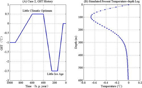
We simulate two scenarios of past ground surface temperature variation. According to the latest report [31] by the Intergovernmental Panel on Climate Change (IPCC), the global surface temperature in recent years (1901–2012) has increased 0.89 ± 0.19 (°C). Case 1 simulates this temperature increase. Case 2 assumed GST history with a ‘Little Climatic Optimum’ from past 400 years to past 600 years, a ‘Little Ice Age’ from past 150 years to past 250 years, and a linear temperature rise from past 50 years to past 150 years. This synthetic GST model is applied by Shen and Beck [32]. The main purpose of this case is to simulate climate change associated with typical climatic events.

Case 1. Linear variation of GST formulated as linear increasing function (13) $T_0(t)=\{\begin{array}{l}-0.01t\text{, }0<t\le 100\\ -1,100<t\le 1000\end{array}.$(13) Case 2. 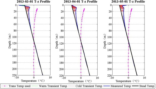GST history with ‘Little Climatic Optimum’, ‘Little Ice Age’, and linear temperature rise (14) $T_0(t)=\{\begin{array}{l}0,0<t\le 50\\ -0.025t+1.25,50<t\le 150\\ -2.5,150<t\le 250\\ 0.02t-7.5,250<t\le 400\\ 0.5,400<t\le 600\\ -0.005t+3.5,600<t\le 900\\ -1,900<t\le 1000\end{array}.$(14) We use Equation (3) to generate the synthetic transient ground temperature profile for each case (see Figures 1 and 2). Figure 1(A) shows stable temperature associated with a relatively gentle climate one century ago and then an incline in GST for the most recent 100 years associated with global warming. Figure 1(B) shows a present temperature distribution profile with depth for the final year of simulation. Similarly, Figure 2(A) shows the GST history in the past 1000 years and Figure 2(B) shows the corresponding simulated present temperature measurement. We assumed ground temperature is measured every 10 m in a borehole (shows as ‘dots’ in Figures 1 and 2(B)). To suppress temperature oscillation in recent times, we use time $\tau =\text{ln}(t)$ rather than normal time t. In τ time space, time points are denser near recent times and sparser towards the end. This adaptive time scheme allows us to have a high-resolution time interval for recent GST. Since we set present time t₀ ≈ 0, we choose τ₀ = −18 to keep t₀ as t₀= ln(τ₀) = ln(−18) ≈ 0. The time variable τ ranges from −18 to ln(t_p) and has equal time step Δτ = 0.1.

Figure 1. Prescribed synthetic GST variation-plotted on the left and simulated present transient ground temperature profile plotted on the right.

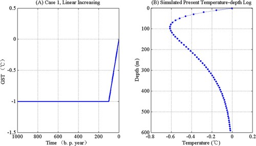
Figure 2. Prescribed synthetic GST variation-plotted on the left and simulated present ground temperature profile plotted on the right.

Since the input data include noises from temperature measurements, we add random noise data $\tilde{h}(z_i)=h(z_i)+\sigma \cdot \text{rand}(i)$ to the simulated ground temperature profiles. Here h(z_i) is the exact data and rand(i) is a random number between [−1, 1], and the magnitude σ denotes the noise level. We use two noise levels of σ = 0.01, 0.1°C, which is typical according to precision of thermistor thermometer sensor [33,34], although some systems produce noise $\sigma \approx 0.001$°C [35].

In order to conduct performance analysis, we utilize the RMSE formula: (15) $\text{RMSE}=\sqrt{\frac{1}{K}\sum _{k=1}^K{(T_k-T_k^{\ast })}^2}$(15) where K is the number of distributed points on the time interval [t₀, t_max], and T_k, T_k* are the exact and approximated surface temperature at these points, respectively.

3. Results

3.1. Ground surface temperature and temperature with depth (T-z log)

To illustrate the application of two methods to the above-described synthetic cases, we recover GSTs under different noise levels. Figure 3(A,B) shows the reconstructed GSTs for Case 1, with noise level 0.01 and 0.1°C of input ground temperature data, respectively. Under the small noise level σ = 0.01°C, GSTs reconstructed by both SVD and Tikhonov methods can track the amplitude and time frame of the warming signal. Our numerical experiment shows that both SVD and Tikhonov method matches the GST in recent 600 years. Both recovered GSTs slightly deviate from prescribed GST at start time (1000 years before present). The difference between SVD and Tikhonov methods is not pronounced, and both methods can robustly reconstruct GST signals.

Figure 3. Estimated GST by SVD method and Tikhonov method for the Case 1 with noise level σ = 0.01°C (A) and σ = 0.1°C (B), and Case 2 with noise level σ = 0.01°C (C) and σ = 0.1°C (D). The uncertainties of GSTs are shown by a dark grey band (SVD method) and light grey band (Tikhonov method) around GSTs.

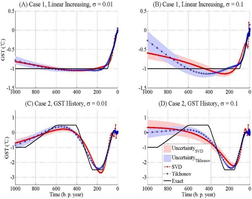
Both methods fail to recover the GST Case 1 with the higher noise level (σ = 0.1°C) (Figure 3(B)). However, the GST estimated using Tikhonov methods follows the prescribed temperatures more closely for the recent 80 years of recovery. GST recovered using the Tikhonov method oscillates around prescribed GST with a smaller amplitude near the end of the time interval. The SVD method shows false oscillations with higher amplitude near current times and further deviates from exact GST under the high noise level. Our experiment shows that the noise level associated with temperature measurement error can significantly affect the inversion ability for both regularization methods towards the end of the time interval (1000 B.P.).

Recovered GSTs for Case 2 are shown on Figure 3(C,D). The ‘Little Climatic Optimum’ and ‘Little Ice Age’ (shown in Figure 2(A)) are two main climatic events to be reconstructed in Case 2. GST reconstructed by Tikhonov method more closely matches these two climatic events than the SVD method (Figure 3(C)). GST recovered by SVD shows false oscillations near the present time and shorter climatic signal of ‘Little Ice Age’. The SVD method is unable to recover ‘Little Climatic Optimum’ signal under high noise level. GST recovered using the Tikhonov method oscillates around prescribed GST with a smaller amplitude and more closely matching the warming trend and steady temperatures in recent 200 years. This experiment suggests that the Tikhonov method can track the GST signal more closely than SVD. For higher noise levels both SVD and Tikhonov methods can reconstruct general climatic trend specifically for time intervals of 400 years to 1000 years before present (Figure 3(D)).

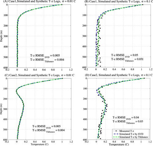
As a verification of the recovered GST signal, we simulated transient ground temperature profiles at the present time and compared them with prescribed borehole temperature for both cases using SVD and Tikhonov methods (Figure 4). The RMSEs between simulated and prescribed Temperature-depth profiles (T-z logs) are also shown in Figure 4. We applied Equation (3) to compute the borehole temperature affected by recovered GST variation. In both cases with the small noise level (σ = 0.01°C) simulated T-z profiles almost replicate the synthetic measured T-z profile, for noise level (σ = 0.1°C) the reconstructed profiles further deviate from the prescribed T-z profiles. In any case, Tikhonov method slightly outperforms the SVD.

Figure 4. Simulated present (t = 0) borehole temperature using recovered GST and comparison with prescribed present borehole logs.

3.2. The root mean square errors and regularization parameters

RMSEs of recovered GSTs and induced T-z profiles for both cases and methods are summarized in Table 1. We add noises of different levels from small noise (σ = 0.001°C) to high noise (σ = 0.5°C) to illustrate the sensitivity of methods. The RMSEs between prescribed and simulated GSTs are increasing with higher noise level (Table 1). In any case, RMSEs of the SVD method are higher than the RMSEs of the Tikhonov method. The truncation number (TN) indicates the number of eigenvectors left as a result of truncation in the SVD method. Tikhonov method shows a better performance in any of two cases (Table 1).

Table 1. RMSEs of GST and induced T-z profiles for synthetic cases by SVD and Tikhonov methods.

	RMSEs	RMSEGST		RMSET-z
Cases	Methods	SVD	Tikhonov	SVD	Tikhonov
Case 1	σ = 0.001	0.0117	0.0039	0.0017	0.0014
	σ = 0.01	0.0584	0.0195	0.0055	0.0049
	σ = 0.1	0.2931	0.0739	0.0485	0.0391
	σ = 0.5	1.4655	0.3758	0.2478	0.2296
Case 2	σ = 0.001	0.5872	0.2438	0.0013	0.0009
	σ = 0.01	0.6684	0.2625	0.0057	0.0041
	σ = 0.1	0.6977	0.2947	0.0437	0.0414
	σ = 0.5	0.7249	0.3268	0.1213	0.1079

We use both GCV and L-curve criteria to choose regularization parameters for the Tikhonov method. Table 2 includes selected regularization parameters for both the Tikhonov and SVD method, and corresponding RMSEs of recovered and prescribed GST for Case 1 and Case 2. Our analysis indicates that L-curve criterion gets slightly better results than GCV in both synthetic methods for all noisy disturbed cases according to RMSEs (Table 1).

Table 2. Regularization parameters for SVD and Tikhonov methods of synthetic cases by L-curve and GCV method.

		SVD		Tikhonov, L-curve		Tikhonov, GCV
Cases	Methods	Truncated number	RMSEGST	α	RMSEGST	α	RMSEGST
Case 1	σ = 0.001	8	0.0117	0.0007	0.0039	0.0001	0.0140
	σ = 0.01	7	0.0584	0.0044	0.0195	0.0015	0.1793
	σ = 0.1	5	0.2931	0.0654	0.0739	0.0287	0.1321
	σ = 0.5	2	1.4655	0.0938	0.3758	0.0371	0.5279
Case 2	σ = 0.001	13	0.5872	0.0012	0.2438	0.0005	0.3477
	σ = 0.01	10	0.6684	0.0018	0.2625	0.0034	0.3621
	σ = 0.1	2	0.6977	0.0333	0.2947	0.0261	0.2957
	σ = 0.5	2	0.7249	0.0689	0.3268	0.0490	0.3586

Tikhonov and SVD methods use different constraints to achieve the desired optimal solutions of regularization. With the noise level increasing, the SVD method keeps fewer singular values and the corresponding singular vectors (see Truncated Number (TN) shown in histograms in Table 1). The number of retained singular values depends on the specific problem and its instability. The instability of the inverse problem is amplified with increasing noise levels. The SVD truncation discards vectors representing noises in the model space, i.e. GST signal, and remain vectors conserving the most part of GST signal.

Similarly, Tikhonov method chooses larger regularization parameters under higher noise level (Table 2). According to Equation (8), the Tikhonov method minimizes weighted combination of the residual norm $\mathit{A}\mathit{m}-{\mathit{d}}_2$ and the side constraint ${\mathit{m}}_2$, where the regularization parameter α controls the weight given to these two norms. The residual norm $\mathit{A}\mathit{m}-{\mathit{d}}_2$ represents the differences between the simulated present T-z log computed from the corresponding GST and the prescribed T-z log. 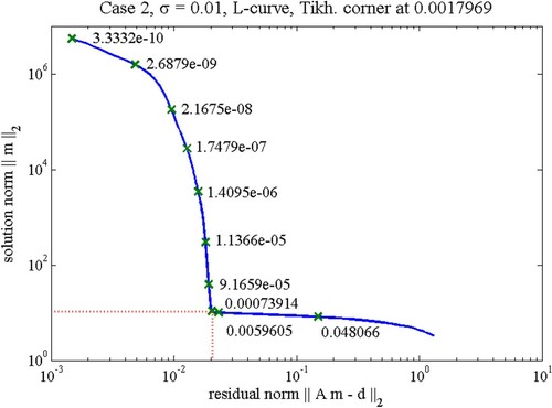The side constraint ${\mathit{m}}_2$ represents the norm of recovered GST signal. The regularization parameter α seeks for the compromise between these two quantities, which is the principle of the Tikhonov method [6,27]. We illustrate an example of both norms by characteristic L-curve for Case 2 with a small noise level σ = 0.01°C in Figure 5. We separated vertical and horizontal parts of the L-curve to represent the regularized solution norm ${\mathit{m}}_2$ and the corresponding residual norm $\mathit{A}\mathit{m}-{\mathit{d}}_2$. Figure 5 shows how sensitive these two norms to the changes in the regularization parameter α. Increasing α illustrates the convergence of the Equation (8). It is clear from Figure 5 that greater α favours a smaller solution norm at the cost of a large residual norm, where small α has the opposite effect [21]. Here, the L-curve displays the trade-off between minimizing the residual norm and side constraint of model parameter m. The optimal regularization parameter is chosen at the corner of L-curve where the combination of residual norm and solution norm reaches their minimum. The misfit between simulated and synthetic logs for both SVD and Tikhonov method (Table 1) verifies the effectiveness of the Tikhonov method to better constraint the residual norm.

Figure 5. L-curve for Tikhonov regularization parameter selection of Case 2. The solid line is the L-curve with several value of iterative regularization parameter marked by ‘x’ mark. Corner noted by dashed line is the best selection of regularization parameter which is α = 0.0018.

4. Field example

4.1. Sites description

Wudaoliang borehole is located in the Wudaoliang Meteorological Station. Vegetation type of this region is Alpine desert with coverage of 10%. Characteristics of contemporary climate change in this region have been investigated based on observational data of air temperature and precipitation [36], which has just cover a period of 1930s to 1998. A study of thawing and freezing processes of the active layer in Wudaoliang region shows that heat is transferred mainly via conductive flow [37]. So this site is suited to apply Borehole Paleothermometry since the main assumption of this method is that we avoid the heat convention because of its minor influence on the temperature log.

Location of the Wudaoliang borehole and some basic information is summarized in Table 3.

Table 3. Basic data and Permafrost depth.

Borehole designation	N Latitude	E Longitude	Elevation, m	Drilling start time	Drilling end time	Depth to 0°C, m
WDL (Wudaoliang)	35°13'21.22"	93° 5'24.00"	4668	24 October 24 2012	6 November 2012	68.4

The duration of drilling of Wudaoliang borehole is 14 days. The total depth of this borehole is 120 m. Thermistor and multimeter are used for temperature measurement with an accuracy of 0.1°C. Temperature measurements were made at depth intervals of 0.5 m between 0.5–5, 1 m of 5–15m, 2 m of 22–40m, 5 m of 40–60m, 10 m of 60–120 m. Figure 6 illustrates the temperature-depth profiles of Wudaoliang borehole and from which we can see roughly the warming trend of the last century.

Figure 6. Temperature-depth profiles of measured temperature on the Wudaoliang borehole (dashed lines). The solid lines represent extrapolations. The shaded area represents anomalous temperature resulting from surface ground temperature variations and its value represented by point marker with dotted line, which start below 12 m.

4.2. Results

We use the temperature-depth log of Wudaoliang borehole measured on 12 July 2013 to reconstruct the past GST history of Wudaoliang area. Since this borehole is just located in Wudaoliang meteorological station, it is sensible to compare the inversion results with air temperature observation of Wudaoliang station. The impact of errors and noise on the inversed GST is demonstrated by the variance of the estimated GST.

The inferred GST history by the SVD method is shown in Figure 7(a). The number of the singular values retained in the SVD reconstructions is 3. We compare the reconstructed GST variation with the nearest surface air temperature (SAT) trend of Wudaoliang station. Figure 7(b) shows the T-z profile that calculated from the estimated GST histories. The a posteriori temperature values fall within 0.1°C of the measured values with the RMS error of 0.0419.

Figure 7. (a) Estimated GSTH for Wudaoliang by SVD method. The uncertainty of GST is shown by a light grey band around GST. (b) Measured and posteriori T-z profiles for the Wudaoliang data, corresponding to the GST histories by SVD method.

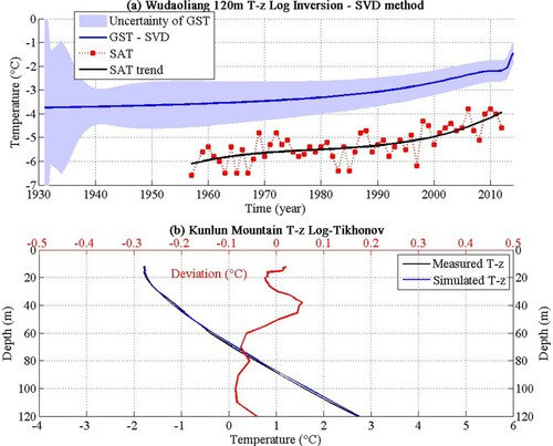
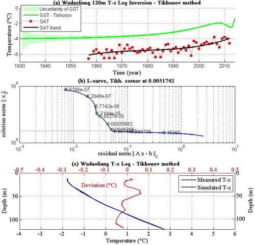
Figure 8(a) gives the inferred GST history by the Tikhonov method. The inversion result of the Tikhonov method not only shows the long-term GST trend but also the recent temperature fluctuation, which is confirmed by observed SAT of the time interval of 2008–2012 year. Figure 8(c) shows the T-z profile that calculated from the estimated GST histories. Except for the shallow 12-m depth, the a posteriori temperature values fall within 0.08°C of the measured values with the RMS error of 0.0305. This RMS error shows the improved Tikhonov method has a better simulation of T-z profile than the SVD method, which indirectly indicated the more robust reconstruction of past ground surface temperature history. Figure 8(b) shows the process of choosing the best regularization parameter by L-curve method and finally figure out the best Tikhonov regularization parameter of 0.0052.

Figure 8. (a) Estimated GSTH for Wudaoliang with the Tikhonov method. The uncertainty of GST is shown by a dark grey band around GST. (b) L-Curve rule for choosing regularization parameter of Tikhonov regularization; (c) Measured and posteriori T-z profiles of Wudaoliang borehole, corresponds to the GST histories by Tikhonov method.

Both the similarities and differences that can be seen in inversions of the same T-z data by both SVD and Tikhonov are displayed in Figure 9. The inversion results show that 83 years ago the ground surface temperature was about −4°C. We use the standard method [1] to estimate the steady-state temperature of 300 years ago so we get a similar steady temperature of the start time for both SVD and Tikhonov method. The recent GST we get by SVD method is −2.06 (±0.4)°C and the GST we get by Tikhonov method is −2.46 (±0.1)°C.

Figure 9. Estimated GSTHs for Wudaoliang by the SVD method and Tikhonov method show the similarities and differences that appear in inversions of the same borehole data by two different methods.

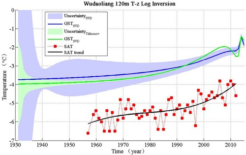
Although the whole warming GST history trends of two methods are the similar that the GST increase from about −4°C to about −2.26°C, but they act differently in recent 20 years. The GST by SVD method keeps increasing until around 2010 year and has a relatively unchanged period and then increases again. The Tikhonov method induced GST history a signal of temperature fluctuation in the period from 2000 to 2013. The SAT trend from Wudaoliang station also show an SAT oscillation from 2008 to 2012 year, which gives assistant proof to the GST variation by the Tikhonov method. Also the better fit between simulated and measured T-z log indicate the higher degree of reliability of the Tikhonov method.

Wudaoliang borehole site shows the warming trend and the warming become intensify start from 1980s (Figure 9). Table 4 summarizes the total GST variation we reconstructed by Borehole Paleothermometry from Wudaoliang borehole and they are the average of results of SVD and Tikhonov methods.

Table 4. Climate change and geothermal gradients parameters from observation boreholes.

Borehole designation	T0, °C	Gradients, °C/km	Inversion time, year	Warmer, °C	ΔT, °C	Tgr, °C
WDL (Wudaoliang)	−4.03 (±1.5)	56.18 (±.03)	83	1.77 (±1.6)	2.02 (±1.6)	−2.26 (±.1)

The reconstructed GST variation of Wudaoliang exhibits the same trend with SAT observation but has a different misfit of 2°C. Borehole temperature is the response of ground surface temperature but not the overlying air temperature [38,39,40]. GST and SAT can change differently with time due to the different surface conditions, such as duration of snow cover, snow time, land use, vegetation development and changes, and also soil moisture level [41–45]. According to the observation records from Wudaoliang Meteorological Station, we know that there are almost no snow cover on Wudaoliang, so the misfit between GST and SAT of Wudaoliang may come from the surface energy budgets processes and local topography.

5. Discussion

Reconstructed ground surface temperature is affected by measurement noise [46]. The uncertainty of reconstructed ground surface temperature increases with higher noise level (see Figure 3). This is due to the truncated number of singular values in the SVD method and the regularization parameter in the Tikhonov method. The resolving power, that is, the ability to detect past climatic events utilizing present borehole temperature measurements, is limited and poor when measurement noise levels are higher than 0.1°C. When measurement noise increases, we should use stronger regularization, which means a larger regularization parameter in the Tikhonov method or smaller truncated number in SVD method to suppress the effect of noises. The resolving power is also sensitive to the vertical distribution of the measurements, temperature measurements uncertainty, the inclusion of a local meteorological records, and the duration of a monitoring experiment [46]. The resolving power of borehole temperature measurements is relatively poor in comparison with other climatic-reconstruction methods such as tree-ring or isotope methods [5,46]. This is mainly due to the physical nature of the heat diffusion process [46]. The analytical results on resolution power of paleoclimate signal in the underground temperature field are theoretically studied and presented by Demezhko and Shchapov [47].

The resolving power of borehole temperature data to resolve past climatic events is also decreasing with time going backward due to the temporal smearing effect of the ground. Therefore, it is important to quantify the degree of temporal smearing of the past climatic changes from measured borehole temperatures. To investigate the duration of the climatic event that can be reconstructed from measured borehole temperatures, we use the Tikhonov method. Here, we use Dirac’s delta function (δ) as an input GST signal to estimate the resolving power of the Tikhonov method. This signal is difficult to reconstruct since extremely fine number of discrete time steps is needed to adequately simulate the shape of δ-function in a numerical code. Instead, we use a Δ-function (shown in Figure 10) as input GST signal, (16) $T_0(t)=\mathrm{\Delta }(t,{\eta }_0).$(16) Here, η₀ is the time when the climatic event is happened before present, Δτ is the half of the width of Δ-function, and Δm is the height of Δ-function. We use the Tikhonov method to reconstruct GST signal of Δ-function. The recovered GST is called a resolving function. A quantity known as the spread is defined as the width of the resolving function, computed as the distance between two time points when GST attain half of the maximum value of the resolving function. The resolving function and a ‘spread’ are shown on Figure 11. We can reconstruct the climatic event that happened 100 years ago for the small noise level (σ = 0.001°C) only if the duration of this climatic event is more than 61 years (see Figure 11). It is clear that the reconstructed GST, shown as a curve on Figure 11, does not fully reconstruct prescribed GST (black curve on Figure 11), but the moving average of prescribed GST in time interval longer than 61 years.

Figure 10. Illustration of Δ-function. Here, Δτ is the half of the width of Δ-function, and Δm is the height of Δ-function.

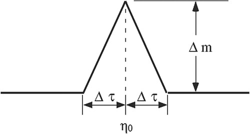
Figure 11. Illustration of resolving function and ‘spread’.

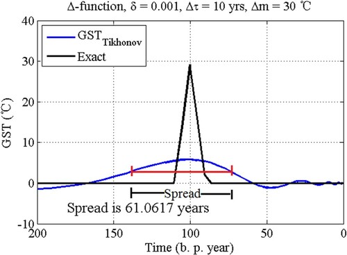
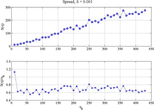
Spread, noted as S(η₀) provides a measure of the detail that can be resolved at time η₀. Climatic events occurring in the vicinity of η₀ with a duration less than S(η₀) cannot be resolved by the available borehole temperature data. Our example in Figure 12 confirms that we can only recover the average of true GST history from borehole temperature profiles. The recovered GST at some time point η₀, which is not the real GST signal but the average of true GST that happened in time interval of vicinity that longer than spread. Figure 12 shows the behaviour of spread S(η₀) and fractional spread S(η₀)/η₀ when input noise level σ = 0.001°C. The spread is increasing with the climatic event happened at time η₀, so the duration of the past climatic event is increasing with time going backward. Fractional spread shows a stable level with increasing η₀ (Figure 12(B)). The average fractional spread is S(η₀)/η₀ = 0.7, which means climatic events occurring around time η₀ with duration of more than 0.7η₀ can be resolved. This rule helps us to understand the reconstructed GST signal that provides the averaged real GST of nearby 0.7η₀ years.

Figure 12. Sensitivity of the spread S(η₀) and the fractional spread S(η₀)/η₀ to the climatic event’s happen time η₀.

There are several methodological limitations in this study. First, we illustrated how to extract transient ground surface temperature variation of borehole temperature profiles skipping that this signal needs to be separated from measured steady-state temperature, when dealing with actual borehole temperature profile [1]. Second, we assume the deep borehole temperature measurement is already stable after drilling. The drilling process adds significant noise to the temperature of a newly created borehole [48]. Thus the measurements must be ‘corrected’ for drilling disturbance effect before using the borehole Paleothermometry method to infer past ground surface temperature. Third, the diffusivity must be chosen carefully depending on the lithology of the drilled borehole. Since we do not consider the nonhomogeneous ground materials, this method is more suitable for boreholes in permafrost region or in rock ground. Finally, after obtaining the measured borehole temperature profiles, we use the temperature below 15 or 20 m to reconstruct rough past GST variation of low spatial resolution. By doing this eliminated the complex influence of the active layer on the borehole thermal regime.

6. Conclusion

In this research, we developed a new borehole Paleothermometry method called the Tikhonov method. This method initially applied the Tikhonov regularization technique to obtain a stable past GST by analyzing borehole temperature profiles. Two synthetic tests, linear increase and GST history, verifying that the Tikhonov method induced GST history are more robust and dependable. We compare both the SVD method and Tikhonov method since they are based on same theoretical framework of parameterized formulation. By adding random noises with different noise levels between 0.01 and 0.1°C we compare the root mean square errors of inversed GST variation by both the SVD method and Tikhonov method. After numerical simulations, we use both two methods to reconstruct the past GST of Wudaoliang Meteorological Station borehole site. The recent 60 years GST trend are consistent with SAT variation trend get from Wudaoliang station with value misfit resulted in local topography and ground surface energy budgets. Considering the above results, we obtain the following conclusions:

• The Tikhonov method can get robust GST results when using a noisy borehole temperature log.

• Compared with the SVD method, this improved Tikhonov method shows significantly smaller errors in the synthetic tests.

• The Tikhonov method can successfully suppress the oscillation shown in recent times.

• The L-curve criterion selects a more appropriate regularization parameter for the Tikhonov method in our synthetic cases.

• Reconstructed GST signal by Tikhonov method provides the averaged real GST of nearby 0.7η₀ years.

• Inversion results of SVD and Tikhonov methods show the increasing trend of 1.8 (±1.6)°C in the past 83 years of Wudaoliang and the major warming started from 1980s. The inversion result of recent GST fluctuation from 2008 to 2012 year that we get from the Tikhonov method is confirmed by SAT observation of Wudaoliang Meteorological Station.

We have tested the method with several real borehole data and the results are confirmed by the observed meteorological data and the reconstruction results by other proxy indicators. We are currently sorting out these results.

Acknowledgement

The data of Wudaoliang borehole site is provided by Professor Lin Zhao.

Disclosure statement

No potential conflict of interest was reported by the author(s).

Additional information

Funding

This research has been supported by the National Natural Science Foundation of China under [Grant Number 41801029].

References

- Lachenbruch AH, Marshall BV. Changing climate: geothermal evidence from permafrost in the Alaskan arctic. Science. 1986;234:689–696.
- Mareschal J-C, Beltrami H. Evidence for recent warming from perturbed geothermal gradients: examples from eastern Canada. Clim Dyn. 1992;6:135–143.
- Shen PY, Beck AE. Least squares inversion of borehole temperature measurements in functional space. J Geophys Res: Solid Earth. 1991;96(B12):19965–19979.
- Pollack HN, Huang S. Climate reconstruction from subsurface temperatures. Annu Rev Earth Planet Sci. 2000;28(1):339–365.
- Bodri L, Cermak V. Borehole climatology: a new method how to reconstruct climate. Amsterdam: Elsevier; 2011.
- Engl HW, Hanke M, Neubauer A. Regularization of inverse problems. Dordrecht: Springer Science & Business Media; 1996.
- Bukharove TI, Nagornov OV, Tyuflin SA. The application conditions for paleotemperature reconstructions based on the borehole measurements. Recent Adv Fluid Mech Therm Eng. 2015: 36–40.
- Wang Y, Zhang Y, Lukyanenko D, et al. Recovering aerosol particle size distribution function on the set of bounded piecewise-convex functions. Inverse Probl Sci Eng. 2013;21:339–354.
- Zhang Y, Hofmann B. On the second-order asymptotical regularization of linear ill-posed inverse problems. Appl Anal. 2020;99:1000–1025.
- Gong R, Hofmann B, Zhang Y. A new class of accelerated regularization methods, with application to bioluminescence tomography. Inverse Probl. 2020;36:055013.
- Liu J, Zhang T. Fundamental solution method for reconstructing past climate change from borehole temperature gradients. Cold Reg Sci Technol. 2014;102:32–40.
- Beltrami H, Mareschal J-C. Recent warming in eastern Canada inferred from geothermal measurements. Geophys Res Lett. 1991;18:605–608.
- Tikhonov AN, Arsenin VY. Methods for solving ill-posed problems. New York: Scripta Series in Mathematics; 1979.
- Wahba G. A survey of some smoothing problems and the method of generalized cross-validation for solving them. Proceedings of Symposium, Wright State University, Dayton, Ohio. In: Applications of statistics. Amsterdam: North-Holland; 1977. p. 507–523.
- Craven P, Wahba G. Smoothing noisy data with spline functions. Numer Math. 1978;31(4):377–403.
- Hansen PC. Numerical tools for analysis and solution of Fredholm integral equations of the first kind. Inverse Probl. 1992b;8:849–872.
- Hansen PC. Rank-deficient and discrete ill-posed problems. Lyngby: Technical University of Denmark; 1996.
- Rath V, Mottaghy D. Smooth inversion for ground surface temperature histories: estimating the optimum regularization parameter by generalized cross-validation. Geophys J Int. 2007;171:1440–1448.
- Lawson CL, Hanson RJ. Solving least squares problems. Philadelphia (PA): SIAM; 1974; First published by Prentice-Hall.
- Hansen PC, O'Leary DP. The use of the L-curve in the regularization of discrete ill-posed problems. SIAM J Sci Comput. 1993;14(6):1487–1503.
- Hansen PC. Regularization tools: a Matlab package for analysis and solution of discrete ill-posed problems. Numer Algorithms. 1994;6(1):1–35.
- Jafarov EE, Marchenko SS, Romanovsky VE. Numerical modeling of permafrost dynamics in Alaska using a high spatial resolution dataset. Cryosphere. 2012;6(3):613–624.
- Carslaw HS, Jaeger JC. Conduction of heat in solids (2nd Ed). Oxford: Oxford University Press; 1959.
- Vasseur G, Bernard PH, Van de Meulebrouck J, et al. Holocene paleotemperatures deduced from geothermal measurements. Palaeogeogr Palaeoclimatol Palaeoecol. 1983;43:237–259.
- Lanczos C. Linear differential operators. New York: D. van Nostrand; 1961.
- Jackson DD. Interpretation of inaccurate, insufficient, and inconsistent data. Geophys J Roy Astr Soc. 1972;28:97–109.
- Menke W. Geophysical data analysis, international geophysical series 45. San Diego (CA): Academic Press; 1989.
- Groetsch CW. The theory of Tikhonov regularization for Fredholm equations of the first kind. Boston (MA): Pitman (Advanced Publishing Program); 1984.
- Hansen PC. Analysis of discrete ill-posed problems by means of the L-curve. SIAM Rev. 1992a;34:561–580.
- Hansen PC. The L-curve and its use in the numerical treatment of inverse problem. In: Johnston P, editor. Computational inverse problems in electrocardiology, advances in computational bioengineering series, vol. 4. Southampton: WIT Press; 2000. p. 119–142.
- Stocker T, Qin D, Plattner G-K, et al. Climate change 2013: the physical science basis. Cambridge/New York: Cambridge University Press; 2014.
- Shen PY, Beck AE. Paleoclimate change and heat flow density inferred from temperature data in the superior Province of the Canadian shield. Palaeogeogr Palaeoclimatol Palaeoecol. 1992;98(2):143–165.
- Liu J, Shen Y, Zhao S. High-precision thermistor temperature sensor: technological improvement and application. J Glaciol Geocryol. 2011;33(4):765–771.
- Shen Y, Liu J, Zhao S. Long-term stability of thermomertric thermistor sensor sklfse-ts used at low temperature. J Glaciol Geocryol. 2012;34(4):891–897.
- Clow GD. USGS polar temperature logging system, description and measurement uncertainties. Rocky Mountain Geographic Science Center; 2008.
- Zhu W, Chen L, Zhou Z. Several characteristics of contemporary climate change in the Tibetan plateau. Sci China D: Earth Sci. 2001;44(1):410–420.
- Zhao L, Cheng G, Li S, et al. Thawing and freezing processes of active layer in wudaoliang region of Tibetan plateau. Chin Sci Bull. 2000;45(23):2181–2187.
- Gosnold W, Todhunter P, Schmidt W. The borehole temperature record of climate warming in the mid-continent of North America. Glob Planet Change. 1997;15(1):33–45.
- Smerdon JE, Pollack HN, Cermak V, et al. Air-ground temperature coupling and subsurface propagation of annual temperature signals. J. Geophys Res: Atmos. 2004;109(D21):1–10.
- Pollack HN, Smerdon JE, Keken PE. Variable seasonal coupling between air and ground temperatures: A simple representation in terms of subsurface thermal diffusivity. Geophys Res Lett. 2005;32(15):L15405.
- Stieglitz M, Dery SJ, Romanovsky VE, et al. The role of snow cover in the warming of Arctic permafrost. Geophys Res Lett. 2003;30(13):1721.
- Hu Q. How have soil temperature been affected by the surface temperature and precipitation in the eurasian continent? Geophys Res Lett. 2005;32(14):L14711.
- Bartlett MG, Chapman DS, Harris RN. Snow and the ground temperature record of climate change. J Geophys Res. 2004;109(F4):F04008.
- Smerdon JE, Beltrami H, Creelman C, et al. Characterizing land surface processes: A quantitative analysis using air-ground thermal orbits. J Geophys Res: Atmos. 2009;114(D15102):1–11.
- Smerdon JE, Pollack HN, Cermak V, et al. Daily, seasonal, and annual relationships between air and subsurface temperatures. J Geophys Res: Atmos. 2006;111(D7):1–12.
- Clow GD. The extent of temporal smearing in surface-temperature histories derived from borehole temperature measurements. Glob Planet Change. 1992;6(2):81–86.
- Demezhko DY, Shchapov VA. 80,000 years ground surface temperature history inferred from the temperature–depth log measured in the superdeep hole SG-4 (the Urals, Russia). Glob Planet Change. 2001;29:219–230.
- Clow GD. A Green's function approach for assessing the thermal disturbance caused by drilling deep boreholes in rock or ice. Geophys J Int. 2015;203(3):1877–1895.