
 ?Mathematical formulae have been encoded as MathML and are displayed in this HTML version using MathJax in order to improve their display. Uncheck the box to turn MathJax off. This feature requires Javascript. Click on a formula to zoom.
Abstract
We are concerned with the reconstruction of the heat capacity coefficient of a one-dimensional heat equation from a sequence of observations of solutions at a single fixed point. This new direct method reconstructs the principal eigenfunction by extracting its Fourier coefficients from the observations of the solution. The algorithm presented here is an alternative to Krein's inverse spectral theory, minimization and iterative procedures. Error estimates and numerical experiments are presented.
1. Introduction
We are concerned with the reconstruction of the heat capacity coefficient appearing in the one-dimensional heat equation
(1)
(1) from observations of a sequence of temperatures taken at an arbitrary single point, i.e.
where b is a fixed but arbitrary point in
. Here the real values h and H in the boundary conditions describe the constant heat transfer occurring at the endpoints, and
is the initial condition.
We recall that in [Citation1] the idea was to extract the complete spectral data of the operator
, from the observation of a single solution on the boundary, i.e.
and
based on Krein's inverse spectral theory of the string [Citation8,Citation10]. The main difficulty of applying Krein's theory is its requirement of having the full and complete spectral data, which is impossible to extract in practice.
This note implements numerically the new method introduced in [Citation4], which applies to multidimensional partial differential equations, and presents an alternative to methods such as the Gelfand–Levitan or Krein inverse spectral theories, optimal control, minimization methods, Newton's and fixed points methods, see [Citation2,Citation6,Citation7,Citation9,Citation11,Citation12]. It is based on a simple idea of computing the Fourier coefficients of the first eigenfunction which allows for a simple approximating scheme of ρ. However, because ρ is unknown, the Fourier coefficients of the principal eigenfunction are not available as in [Citation4,Citation5], and so the analysis needs to be modified which is the purpose of this note. The main result can be stated as follows:
Theorem 1.1
Let be a basis of
that we take for the initial condition
for
and let
. If
then we can reconstruct
from the map
. In the Neumann case, i.e. h = H = 0, then we also need the mean value of
We now briefly describe the content of the paper. Notations are in Section 2, and in Section 3, the idea on how to reconstruct ρ by computing the first eigenvalue and
from the observation of the solution at one point is given. By solving an auxiliary boundary problem we then find
and deduce the sought coefficient ρ. The Dirichlet and the Neumann cases are examined respectively in Section 4 and Section 5. Convergence is proved in Section 6 while the algorithm is exposed in Section 7. Numerical examples are provided in the last section.
2. Preliminaries
By the Fourier method, the solution of Equation (Equation1(1)
(1) ) can be written as
(2)
(2) where the Fourier coefficients are given by
(3)
(3) and
are eigenfunctions of the Sturm–Liouville operator A defined by
(4)
(4) where
, and
It is also known that A, defined by (Equation4
(4)
(4) ), is a self-adjoint operator acting in the Hilbert space
and its spectrum is discrete and simple. Since
and
then
and
forms an orthonormal basis of
normalized by
In the fifties, Krein used the inverse spectral theory of the string operator which is generated by the differential operator
where
is a Stieljtes measure defined by a nondecreasing function M, which represents the mass of a string, and
is the right derivative at x, see [Citation8,Citation10] for the spectral theory of the string. When
is an absolutely continuous function, the string operator reduces to (Equation4
(4)
(4) ) and
is understood as
and thus, when ρ vanishes on a subinterval, the solution f is a linear function.
We assume that so the Fourier coefficients
in (Equation3
(3)
(3) ) are well defined although the weight
is yet unknown. We still have
and
Remark 2.1
The sum in Equation (Equation2(2)
(2) ) provides a representation of the solution only, although all its terms are unknown. The objective is to use the observation
to extract the Fourier coefficients
and
, whenever they are present, as the
can vanish. Obviously, if a coefficient is not present in the sum then it cannot be extracted.
3. Reconstructing ρ
In principle, to reconstruct ρ it is enough to reconstruct the first eigenfunction , since ρ is a solution of the algebraic equation
(5)
(5) To do so we only need the first eigenvalue
as we already have
for all
To reconstruct
we could use a basis of
say
, to write
(6)
(6) with the hope that we can read the coefficients
from the solution
as done in [Citation4]. Unfortunately, the observation
in (Equation2
(2)
(2) ) contains a different coefficient of the exponential, namely,
(7)
(7) with initial condition
In other words, even if we could extract the whole sequence
from (Equation2
(2)
(2) ), we still cannot reconstruct
by (Equation6
(6)
(6) ), but
(8)
(8) where we used the notation (Equation3
(3)
(3) ). To proceed further we now show how to extract the coefficients (Equation7
(7)
(7) ) from (Equation2
(2)
(2) ).
3.1. Extracting  from observations
To capture from (Equation2
(2)
(2) ), it is enough to use the method of limits, [Citation3], on the sequence of observations or data given by
for a fixed
Assume that
does not change sign, say
and since
the sequence
generated by
is nontrivial and has the asymptotic for large j,
(9)
(9) which yields
(10)
(10) Although the limit is easy to set up, its existence hinges on the facts that
as the first eigenfunction does not vanish inside, and also on
as the functions do not change sign. The limit can then be used to find the sought Fourier coefficients
(11)
(11) From (Equation11
(11)
(11) ), and (Equation8
(8)
(8) ) we have
(12)
(12) Since we have reconstructed
we only need
to deduce ρ. To this end, since we already have
and
it means we have the right-hand side of a rescaled (Equation5
(5)
(5) ), i.e.
(13)
(13) where
which is easily obtained by the Green's function of the boundary value problem
(14)
(14) The existence and uniqueness is given by the following lemma.
Lemma 3.1
If then
and the solution to the boundary value problem (Equation13
(13)
(13) ) exists and is given explicitly by
with
defined by (Equation15
(15)
(15) ). Furthermore, the map
is a bounded operator from
Proof.
If then
from (Equation5
(5)
(5) ) and so
Using the boundary conditions, at
yield the system
which gives a nontrivial solution, i.e.
if and only if its determinant, which is the Wronskian
The same condition also implies that (Equation14
(14)
(14) ) has a unique solution, which we can obtain using the Green's function
(15)
(15) where
. From
and the fact that the Green function is continuous, we deduce that
(16)
(16) with
Once we have reconstructed we can solve (Equation13
(13)
(13) ) to obtain
(17)
(17) Combining (Equation12
(12)
(12) ) and (Equation17
(17)
(17) ) yield
(18)
(18) where
(19)
(19) Recall that the denominator is non zero since
for all
. Thus, we have proved the main result of the paper stated previously in Theorem 1.1.
Remark 3.2
The condition excludes two cases, namely the Dirichlet and the Neumann cases which will be treated separately below. Note that their Green's function is easier to compute.
4. The Dirichlet case
With few modifications, we can also treat the Dirichlet case which corresponds to the limiting case in (Equation1
(1)
(1) ) i.e.
(20)
(20) whose solution is given by
(21)
(21) where
are the eigenfunctions,
(22)
(22) It is readily seen that
otherwise
and clearly all eigenvalues are positive
. The Fourier coefficients are given by
Next, we use the basis
to extract
and the coefficients
from the observation
, from (Equation21
(21)
(21) ) by the method of limits. Using the sequence
we reconstruct
(23)
(23) One of the advantages of the Dirichlet problem is the simplicity of its Green's function. From (Equation22
(22)
(22) ) we have
(24)
(24) From (Equation24
(24)
(24) ) and (Equation23
(23)
(23) ) it follows that
(25)
(25) In order words, we deduce from (Equation25
(25)
(25) )
(26)
(26) Thus after obtaining
and
we can reconstruct
by (Equation26
(26)
(26) ). Thus we have proved the following theorem
Theorem 4.1
In the Dirichlet case we can reconstruct by (Equation26
(26)
(26) ) from the map
for any fixed
where u is a solution of (Equation20
(20)
(20) ).
Remark 4.2
Although we still cannot simplify (Equation26
(26)
(26) ) because it is unknown.
We now work out the Neumann boundary condition which is very different because 0 is an eigenvalue.
5. The Neumann case
Neumann boundary conditions means we have in (Equation1
(1)
(1) ) i.e.
(27)
(27) whose solution is given by
(28)
(28) Here
are the normalized eigenfunctions in
with
and are solutions of
(29)
(29) with eigenvalues
(30)
(30) The Fourier coefficients in (Equation28
(28)
(28) ) are given by
It follows from (Equation28
(28)
(28) ) that
Note we are not looking for the first eigenvalue, as it is already known to be zero. Next, we use the basis
as initial conditions to extract the first coefficients in (Equation28
(28)
(28) ), and use (Equation30
(30)
(30) )
(31)
(31) Next observe that for
(Equation31
(31)
(31) ) reduces to
and the Fourier cosine coefficient of ρin terms of the observation
(32)
(32) Recall that the Fourier cosine series of ρ in
is
Thus we need the value
in order to reconstruct ρ.
Theorem 5.1
In the Neumann case we can reconstruct ρ provided we know and the map
for
Remark 5.2
If we could extract the second eigenvalue, then we can recover ρ by a similar formula to (Equation26
(26)
(26) ) and we would not need the value
6. Convergence
In practice, we can only use a finite sum to approximate
given in (Equation19
(19)
(19) ). Using the notation of section 3, let us denote the approximation of ρ by
(33)
(33) If
then
Note that as
in
it follows that
as
Recall that we have
for 0<x<1 and thus for any interval
such that 0<a<b<1 we have
Then, it follows
where M is defined in (Equation16
(16)
(16) ). Therefore we have proved the following theorem.
Theorem 6.1
defined by (Equation33
(33)
(33) ) converges to ρ on any subinterval of
, i.e.
in
for any
7. Algorithm
The whole reconstruction procedure is based on the infinite limits (Equation10(10)
(10) ) and (Equation11
(11)
(11) ). Since we cannot take them in practice, we shall use the tolerance, ε say, to find a stopping time numerically. Thus from the limit in (Equation10
(10)
(10) ) we have
(34)
(34) where
is determined numerically. We also use the same idea to compute the Fourier coefficients
from the limits in (Equation11
(11)
(11) ). As we shall see in the examples, due to the rapid decay of the exponentials, in general,
We now work out few numerical examples to illustrate the method.
8. Numerical examples
For the sake of simplicity, we shall use Dirichlet and Neumann boundary conditions where the initial condition is chosen from the basis
for the former and
for the latter. The observations of the solution are taken at either
or
and generated by solving (Equation1
(1)
(1) ) using the Crank–Nicholson method up to T. We recall that it follows from (Equation10
(10)
(10) ) that the sequence of ratios
Example 1. Consider
Figure 1. – and
+++.
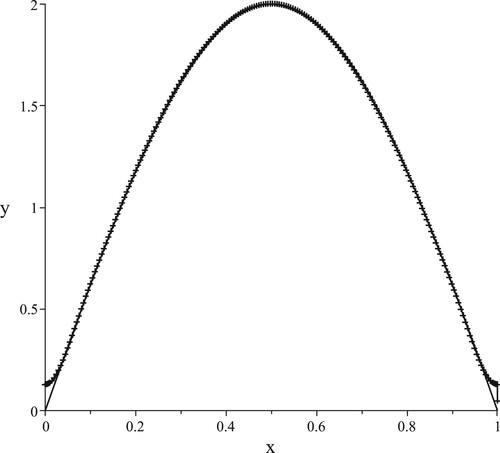
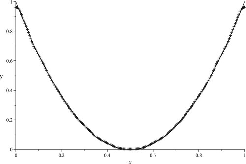
Figure 2. – and
+++
k, r(k)
35, 0.9437854846474063
36, 0.9437854846439294
37, 0.9437854846420766
38, 0.9437854846410607
39, 0.9437854846405333
40, 0.9437854846402476
41, 0.9437854846400894
42, 0.9437854846400063
Thus, tolerance is achieved at time
which means that
. This yields
from
. Next we obtain the sequence of Fourier coefficients by evaluating
0.1794, 7.333 e−16, −0.0390, −3.667e−17, −0.4194e−2, −2.649e−17, −0.1497e−2, 1.111 e−16, −6.936e−4, −4.778e−16, −3.768e−4, −1.235e−16, −2.272e−4, −5.787e−16, −1.474e−4, 4.971 e−16, −1.011e−4, −4.776e−16, −7.232e−5, 9.872 e−16.
Using (Equation26(26)
(26) ) we get
Example 2: We now treat the Neumann case
and so the extra data is
We also know that the first eigenvalue is
and we shall observe the
. To find
use the ratios k, r(k)
284, 0.99996174
285, 0.99998622
286, 0.99998188
287, 1.00001679
288, 1.00000472
289, 1.00033535
290, 0.99944850
291, 1.00031139
292, 1.00000228 we conclude that =3 for
The sequence of Fourier coefficients is seq(c[k],k= 0.20):
1.0000, 3.7746 e−13 , 0.6079, −1.1207e−11, 0.1519, 5.1966 e−11, 0.0674, −1.4377e−10, 0.0379,3.1113 e−10 , 0.0242, −5.8620e−10, 0.0168, 1.0112 e−9, 0.0124, −1.6288e−9, 0.00956, 2.4390 e−9 , 0.0076, −3.2949e−9, 0.0063.
9. Conclusion
We have shown that tools from signal processing can help extract spectral data to reconstruct an unknown weight of a parabolic equation. It also shows that good imaging and non-destructive testing in industry can be achieved with few measurements done with one accurate sensor.
Acknowledgements
The authors sincerely thank the referees for their valuable comments and insight. Both authors also thank KFUPM for its support.
Disclosure statement
No potential conflict of interest was reported by the author(s).
Additional information
Funding
References
- Al-Musallam F, Boumenir A. Recovery of a parabolic equation generated by a Krein string. J Math Anal Appl. 2014;420(2):1408–1415.
- Boumenir A, Ghattassi M, Laleg-Kirati TM. Monitoring the temperature of a direct contact membrane distillation. Math Methods Appl Sci. 2020;43(3):1399–1408.
- Boumenir A, Tuan VK. Recovery of the heat coefficient by two measurements. Inverse Probl Imaging. 2011;5(4):775–791.
- Boumenir A, Tuan VK. Inverse problems for multidimensional heat equations by measurements at a single point on the boundary. Numer Funct Anal Optim. 2009;30(11-12):1215–1230.
- Boumenir A, Tuan VK, Nguyen N. The recovery of a parabolic equation from measurements at a single point. Evol Equ Control Theory. 2018;7(2):197–216.
- Cao K, Lesnic D. Reconstruction of the perfusion coefficient from temperature measurements using the conjugate gradient method. Int J Comput Math. 2018;95(4):797–814.
- Cordaro PD, Kawano A. A uniqueness result for the recovery of a coefficient of the heat conduction equation. Inverse Probl. 2007;23(3):1069–1085.
- Dym H, McKean HP. Gaussian processes, function theory, and the inverse spectral problem. New York: Academic Press; 1976. (Probability and Mathematical Statistics; vol. 31).
- Huntul MJ, Lesnic D, Hussein MS. Reconstruction of time-dependent coefficients from heat moments. Appl Math Comput. 2017;301:233–253.
- Kac IS, Krein MG. On the spectral functions of the string. Amer Math Soc Transl. 1974;103:19–102.
- Kac A. An introduction to the mathematical theory of inverse problems. New York: Springer; 1996. (Applied Mathematical Sciences; vol. 120).
- Lowe BD, Rundell W. An inverse problem for a Sturm-Liouville operator. J Math Anal Appl. 1994;181:188–199.