Sequential estimation of the time-dependent heat transfer coefficient using the method of fundamental solutions and particle filters

Abstract

In many thermal engineering problems involving high temperatures/high pressures, the boundary conditions are not fully known since there are technical difficulties in obtaining such data in hostile conditions. To perform the task of estimating the desired parameters, inverse problem formulations are required, which entail to performing some extra measurements of certain accessible and relevant quantities. In this paper, justified also by uniqueness of solution conditions, this extra information is represented by either local or non-local boundary temperature measurements. Also, the development of numerical methods for the study of coefficient identification thermal problems is an important topic of research. In addition, in order to decrease the computational burden, meshless methods are becoming popular. In this article, we combine, for the first time, the method of fundamental solutions (MFS) with a particle filter sequential importance resampling (SIR) algorithm for estimating the time-dependent heat transfer coefficient in inverse heat conduction problems. Two different types of measurements are used. Numerical results indicate that the combination of MFS and SIR shows high performance on several test cases, which include both linear and nonlinear Robin boundary conditions, in comparison with other available methods.

Keywords:

• Particle filter
• method of fundamental solutions
• inverse heat conduction
• heat transfer coefficient
• Bayesian inference

AMS Classifications:

• 62L12
• 65M12

1. Introduction

In inverse transient heat transfer problems that are solved iteratively, we usually need a direct problem solver that is fast and accurate. Therefore, the development of numerical methods such as meshless methods, especially the method fundamental solutions (MFS) [1], attempting to satisfy these two conditions, became an important task. The MFS is a collocation method where no mesh needs to be generated, and this makes it relatively easy to program and computationally inexpensive. The MFS possesses the same advantages as the boundary element method (BEM), but in addition it does not require any boundary discretization [2]. The limitations are therefore the need for a fundamental solution being explicitly available and the extra ill-conditioning that arises from its meshless character. The MFS has predominantly been applied to stationary heat conduction problems governed by the Laplace, modified Helmholtz or biharmonic PDEs [2–4] and it has produced accurate and stable results. The MFS for the time-dependent linear parabolic heat equation was proposed in [5] and was investigated theoretically and computationally in [6]. From thereon, it has been used in many instances for solving various inverse problems for the parabolic heat equation in one or two-dimensions in fixed or moving boundary domains [7–9].

It is well-known that the heat transfer coefficient (HTC), which characterizes the contribution that an interface makes to the overall resistance of the heat conducting system, it is one of the most important quantities to estimate in heat transfer. Prior to this study, for the resolution of the inverse transient heat conduction problem concerning the determination of the HTC, Masson et al. [10] and Yang et al. [11] applied the conjugate gradient iterative regularization method to estimate the two-dimensional space-dependent HTC. However, especially for nonlinear problems, such gradient methods of minimizing the least-squares gap between the computed and measured data can get trapped in a local minimum and therefore they require a good initial guess. An alternative methodology that can be considered, based on Bayesian inference, [12,13], has a number of distinctive attributes, e.g. it provides statistically meaningful posterior error estimates. In the Bayesian approach to statistics, an attempt is made to utilize all available information in order to reduce the amount of uncertainty present in an inferential or decision-making process. As new information is obtained, it is combined with previous information to form the basis for statistical procedures. The formal mechanism used to combine the new information with the previously available information is known as Bayes' theorem.

In the Bayesian framework, state estimation problems are often solved with the so-called Bayesian filter, which requires relatively low computational demands compared to the Markov chain Monte Carlo (MCMC) algorithm [14]. The most widely known Bayesian filter is the Kalman filter (KF) [15], which is, however, limited to linear models with additive Gaussian noise. Extensions of the KF were developed in the past for less restrictive cases by using linearization techniques [12]. Similarly, sequential Monte Carlo methods have been developed in order to represent the posterior density in terms of random samples and associated weights. Such methods, usually denoted as particle filters among other designations found in the literature, do not require the restrictive hypotheses of KF. Hence, particle filters can be applied to nonlinear systems with non-Gaussian errors [12,16–18].

In 1964, Hammersley and Hanscomb [19] presented a technique that used recursive Bayesian filters, along with Monte Carlo simulations, known as Sequential Importance Sampling (SIS). In this approach, the key idea is to represent the posterior probability function as a set of random samples with associated weights, in order to calculate the estimates based on these samples and weights. Three decades later, Gordon et al. [20] added an extra step, named re-sampling, into the SIS method to avoid a problem known as degeneration of particles. This filter is known as the Sequential Importance Re-sampling (SIR) algorithm [21,22].

In the present study, the objective is to evaluate the performance of the MFS+SIR filter for estimating the time-dependent HTC $\rho (t)$ at time t and to compare it with other methods, which reported unrealistic negative and unstable results. Since we seek to determine a HTC that is time-dependent only, as far as the inverse problem is concerned, the spatial dimensionality of the domain is less relevant. Even so, the fact that the HTC is not treated as a constant parameter offers a more realistic model to various practical applications such as nucleate boiling on cylinders [23], or quenching experiments [24]. We study the sequential estimation of the time-dependent HTC in the inverse heat conduction problem introduced in Section 2. The MFS is used to solve the direct problem sequentially for the SIR filter, as described in Sections 3 and 4. Numerical results presented and discussed in Section 5 indicate that this combination shows good performance in terms of robustness, stability and accuracy compared to other existing methods. Finally, conclusions are made in Section 6.

The mathematical formulation and analysis of this paper can also be extended to higher dimensions [25–28], and numerically analysed, in principle, using the same approach based on the SIR particle filter combined with the MFS [27]. Space-dependent thermal conductivity can also be analysed with the MFS in case it is square-root harmonic [29], or for a piecewise homogeneous layered material [30].

2. Mathematical formulation

In this section, we formulate the mathematical model for the inverse problem of determining a time-dependent Robin HTC. Given a final time of interest $t_f>0$, and a one-dimensional finite slab $\mathrm{\Omega }=(0,1)$, the aim is to find the pair $(T(x,t),\rho (t))$, where $T(x,t)$ represents the temperature for $x\in \mathrm{\Omega }$, $t\in [0,t_f)$, and $\rho (t)\ge 0$ is the time-dependent HTC satisfying: (1a) $\begin{array}{r}\frac{\mathrm{\partial }T}{\mathrm{\partial }t}(x,t)=\frac{{\mathrm{\partial }}^{2}T}{\mathrm{\partial }{x}^2}(x,t),(x,t)\in (0,1)\times (0,t_f),\end{array}$(1a) (1b) $\begin{array}{r}T(x,0)=T^0(x),x\in (0,1),\end{array}$(1b) (1c) $\begin{array}{r}-\frac{\mathrm{\partial }T}{\mathrm{\partial }x}(0,t)+\rho (t)g(T(0,t))=h_0(t),t\in [0,t_f),\end{array}$(1c) (1d) $\begin{array}{r}\frac{\mathrm{\partial }T}{\mathrm{\partial }x}(1,t)+\rho (t)g(T(1,t))=h_1(t),t\in [0,t_f),\end{array}$(1d) where g, $T^0$, $h_0$ and $h_1$ are given functions, and, for simplicity, the heat capacity and thermal conductivity were taken to be constant and equal to unity, whilst the heat source was assumed to be absent. In Equations (1c(1c) $\begin{array}{r}-\frac{\mathrm{\partial }T}{\mathrm{\partial }x}(0,t)+\rho (t)g(T(0,t))=h_0(t),t\in [0,t_f),\end{array}$(1c) ) and (1d(1d) $\begin{array}{r}\frac{\mathrm{\partial }T}{\mathrm{\partial }x}(1,t)+\rho (t)g(T(1,t))=h_1(t),t\in [0,t_f),\end{array}$(1d) ), the right-hand side functions $h_0$ and $h_1$ are usually taken to be zero such that their homogeneous versions model the Newton's or Stefan-Boltzman's law of boundary heat transfer with the environment. Under certain assumptions on the input data, the direct problem given by (1a(1a) $\begin{array}{r}\frac{\mathrm{\partial }T}{\mathrm{\partial }t}(x,t)=\frac{{\mathrm{\partial }}^{2}T}{\mathrm{\partial }{x}^2}(x,t),(x,t)\in (0,1)\times (0,t_f),\end{array}$(1a) )–(1d(1d) $\begin{array}{r}\frac{\mathrm{\partial }T}{\mathrm{\partial }x}(1,t)+\rho (t)g(T(1,t))=h_1(t),t\in [0,t_f),\end{array}$(1d) ) when ρ is known, can be shown to be well-posed [26,31].

In the inverse problem, in order to compensate for the unspecified HTC, we consider some additional information given by [26,32,33] either the boundary temperature measurement, (2) $\begin{array}{r}Y(t)=T(1,t),t\in [0,t_f),\end{array}$(2) or the non-local measurement (3) $\begin{array}{r}E(t)={\int }_{\mathrm{\partial }\mathrm{\Omega }}\mathrm{\Phi }(T(x,t))\mathrm{d}s(x)=\mathrm{\Phi }(T(0,t))+\mathrm{\Phi }(T(1,t)),t\in [0,t_f),\end{array}$(3) where $\mathrm{\Phi }(T)=\int g(T)dT$ is a primitive of the function g governing the linear $(g(\sigma )=\sigma )$ or nonlinear (e.g. radiative $g(\sigma )={\sigma }^3|\sigma |$) boundary heat transfer law [26]. Therefore, in the linear case $g(\sigma )=\sigma$ and $\mathrm{\Phi }(T)=T^2/2$, whilst in the radiative nonlinear case $g(\sigma )={\sigma }^3|\sigma |$ and $\mathrm{\Phi }(T)=T^4|T|/5$. Of course, $E(t)$ represents a boundary integral involving the temperature history over the boundary $\mathrm{\partial }\mathrm{\Omega }$ and it has more physical meaning in higher dimensions. In one-dimension, as calculated in (3(3) $\begin{array}{r}E(t)={\int }_{\mathrm{\partial }\mathrm{\Omega }}\mathrm{\Phi }(T(x,t))\mathrm{d}s(x)=\mathrm{\Phi }(T(0,t))+\mathrm{\Phi }(T(1,t)),t\in [0,t_f),\end{array}$(3) ), $E(t)$ is just a known expression between the unknown boundary temperatures at the ends $x\in \{0,1\}$ of the finite slab.

We finalize this section by mentioning that a typical practical application in which a time-dependent HTC (defined in terms of the heat flux across a surface for a unit temperature gradient) needs to be estimated occurs in the study of forced-convective flow boiling over the outer surface of a heater tube [34]. The nonlinear estimation of a temperature-varying HTC has been considered elsewhere [35].

3. The method of fundamental solutions (MFS)

Only a few MFS applications to time-dependent inverse problems can be found in the literature and moreover, the MFS has rarely been used in conjunction with statistical methods [36]. The fundamental solution of the one-dimensional heat equation (1a) is given by (4) $\begin{array}{r}F(x,t;y,\tau )=\frac{H(t-\tau )}{\sqrt{4\pi (t-\tau )}}{e}^{-(x-y{)}^2/(4(t-\tau ))},\end{array}$(4) where H is the Heaviside function, which is introduced to emphasize that the fundamental solution is zero for $t\le \tau$. Then, based on the MFS, an approximation to the solution $T(x,t)$ can be sought as [6,37], (5) $\begin{array}{rl}{T}_M(x,t)& =\sum _{m=-M+1}^M{c}_m^{(0)}F(x,t;y_0,{\tau }_m)\\ & +\sum _{m=-M+1}^M{c}_m^{(1)}F(x,t;y_1,{\tau }_m),(x,t)\in [0,1]\times [0,t_f],\end{array}$(5) where ${\tau }_m=\frac{(2m-1)t_f}{2m}$ for $m=-M+1,\dots ,M,$ $y_0=-h$ and $y_1=1+h$; h>0 is the distance from the source points to the boundary, and M represents the truncation level of an infinite series expansion whose span is dense in the set of functions satisfying the heat equation (1a(1a) $\begin{array}{r}\frac{\mathrm{\partial }T}{\mathrm{\partial }t}(x,t)=\frac{{\mathrm{\partial }}^{2}T}{\mathrm{\partial }{x}^2}(x,t),(x,t)\in (0,1)\times (0,t_f),\end{array}$(1a) ). The negative times are needed to be included in order to accommodate for the imposition of the initial condition (1b(1b) $\begin{array}{r}T(x,0)=T^0(x),x\in (0,1),\end{array}$(1b) ). More on the linear independence and denseness in $L^2(\{0,1\}\times (0,T))$ of the set of functions $\{F(x,t;y_0,{\tau }_m),F(x,t;y_1,{\tau }_m)\}$ with $({\tau }_m{)}_{m\in \mathbb{Z}}$ dense in $(0,T)$ can be found in [38]. We note that the source points can also be placed at various space locations in the interval $[0,1]$ at fixed time instant(s) outside the interval $[0,t_f]$, see [37], but this selection is actually not needed.

In the direct problem (1a(1a) $\begin{array}{r}\frac{\mathrm{\partial }T}{\mathrm{\partial }t}(x,t)=\frac{{\mathrm{\partial }}^{2}T}{\mathrm{\partial }{x}^2}(x,t),(x,t)\in (0,1)\times (0,t_f),\end{array}$(1a) ) – (1d(1d) $\begin{array}{r}\frac{\mathrm{\partial }T}{\mathrm{\partial }x}(1,t)+\rho (t)g(T(1,t))=h_1(t),t\in [0,t_f),\end{array}$(1d) ), the HTC $\rho (t)$ is known and only the coefficients $c_m^{(0)}$ and $c_m^{(1)}$ for $m=-M+1,\dots ,M$ are unknown and have to be determined by imposing the initial and boundary conditions (1b(1b) $\begin{array}{r}T(x,0)=T^0(x),x\in (0,1),\end{array}$(1b) ) – (1d(1d) $\begin{array}{r}\frac{\mathrm{\partial }T}{\mathrm{\partial }x}(1,t)+\rho (t)g(T(1,t))=h_1(t),t\in [0,t_f),\end{array}$(1d) ). Therefore, selecting the times $t_k=\frac{k\cdot t_f}{M}$ for $k=0,\dots ,M$ and the space points $x_l=\frac{l}{N+1}$ for $l=1,\dots ,N$, we obtain the following system of $(N+2M+2)$ equations with $4M$ unknowns: (6) $\begin{array}{rl}& \sum _{i=0}^1\sum _{m=-M+1}^M{c}_m^{(i)}F(x_l,0;y_i,{\tau }_m)=T^0(x_l),l=1,\dots ,N,\end{array}$(6) (7) $\begin{array}{rl}& -\sum _{i=0}^1\sum _{m=-M+1}^M{c}_m^{(i)}\frac{\mathrm{\partial }F}{\mathrm{\partial }x}(0,t_k;y_i,{\tau }_m)+{\rho }_{k}g(\sum _{i=1}^1\sum _{m=-M+1}^M{c}_m^{(i)}F(0,t_k;y_i,{\tau }_m))=h_0(t_k),\\ & k=0,\dots ,M,\end{array}$(7) (8) $\begin{array}{rl}& \sum _{i=0}^1\sum _{m=-M+1}^M{c}_m^{(i)}\frac{\mathrm{\partial }F}{\mathrm{\partial }x}(1,t_k;y_i,{\tau }_m)+{\rho }_{k}g(\sum _{i=1}^1\sum _{m=-M+1}^M{c}_m^{(i)}F(1,t_k;y_i,{\tau }_m))=h_1(t_k),\\ & k=0,\dots ,M,\end{array}$(8) where ${\rho }_k=\rho (t_k)$ for $k=0,\dots ,M$. The above system can be written in a generic form as: (9) $\begin{array}{r}A(\underset{\_}{c})=\underset{\_}{r},\end{array}$(9) where $\underset{\_}{c}=((c_m^{(0)}{)}_{m=-M+1,\dots ,M},(c_m^{(i)}{)}_{m=-M+1,\dots ,M})$ is the vector of unknowns and $\underset{\_}{r}$ is a known right-hand side vector containing the initial values $(T^0(x_l){)}_{l=1,\dots ,N}$, and the boundary values $(h_0(t_k){)}_{k=0,\dots ,M}$ and $(h_1(t_k){)}_{k=0,\dots ,M}$. The nonlinear vectorial function A contains the fundamental solution (4(4) $\begin{array}{r}F(x,t;y,\tau )=\frac{H(t-\tau )}{\sqrt{4\pi (t-\tau )}}{e}^{-(x-y{)}^2/(4(t-\tau ))},\end{array}$(4) ) and its space derivative $\frac{\mathrm{\partial }F}{\mathrm{\partial }x}(x,t;y,\tau )=\frac{(y-x)H(t-\tau )}{4\sqrt{\pi (t-\tau {)}^3}}{e}^{-\frac{(x-y{)}^2}{4(t-\tau )}}$.

In the inverse problem, the vector $\underset{\_}{\rho }=(\rho (t_k){)}_{k=0,\dots ,M}$ is also unknown and the system of Equations (6(6) $\begin{array}{rl}& \sum _{i=0}^1\sum _{m=-M+1}^M{c}_m^{(i)}F(x_l,0;y_i,{\tau }_m)=T^0(x_l),l=1,\dots ,N,\end{array}$(6) )–(8(8) $\begin{array}{rl}& \sum _{i=0}^1\sum _{m=-M+1}^M{c}_m^{(i)}\frac{\mathrm{\partial }F}{\mathrm{\partial }x}(1,t_k;y_i,{\tau }_m)+{\rho }_{k}g(\sum _{i=1}^1\sum _{m=-M+1}^M{c}_m^{(i)}F(1,t_k;y_i,{\tau }_m))=h_1(t_k),\\ & k=0,\dots ,M,\end{array}$(8) ) is supplemented with the additional information (2(2) $\begin{array}{r}Y(t)=T(1,t),t\in [0,t_f),\end{array}$(2) ) or (3(3) $\begin{array}{r}E(t)={\int }_{\mathrm{\partial }\mathrm{\Omega }}\mathrm{\Phi }(T(x,t))\mathrm{d}s(x)=\mathrm{\Phi }(T(0,t))+\mathrm{\Phi }(T(1,t)),t\in [0,t_f),\end{array}$(3) ) given by (10) $\begin{array}{r}\sum _{i=0}^1\sum _{m=-M+1}^M{c}_m^{(i)}F(1,t_k;y_i,{\tau }_m)=Y(t_k),k=0,\dots ,M,\end{array}$(10) or (11) $\begin{array}{rl}& \mathrm{\Phi }(\sum _{i=0}^1\sum _{m=-M+1}^M{c}_m^{(i)}F(0,t_k;y_i,{\tau }_m))+\mathrm{\Phi }(\sum _{i=0}^1\sum _{m=-M+1}^M{c}_m^{(i)}F(1,t_k;y_i,{\tau }_m))=E(t_k),\\ & k=0,\dots ,M.\end{array}$(11) In this case, instead of Equation (9(9) $\begin{array}{r}A(\underset{\_}{c})=\underset{\_}{r},\end{array}$(9) ) we have the extended version (12) $\begin{array}{r}\tilde{A}(\underset{\_}{c},\underset{\_}{\rho })=\widetilde{\underset{\_}{r}},\end{array}$(12) where the vector $\widetilde{\underset{\_}{r}}$ contains the vector $\underset{\_}{r}$ along with the discretized values in the right-hand side of Equation (10(10) $\begin{array}{r}\sum _{i=0}^1\sum _{m=-M+1}^M{c}_m^{(i)}F(1,t_k;y_i,{\tau }_m)=Y(t_k),k=0,\dots ,M,\end{array}$(10) ) or Equation (11(11) $\begin{array}{rl}& \mathrm{\Phi }(\sum _{i=0}^1\sum _{m=-M+1}^M{c}_m^{(i)}F(0,t_k;y_i,{\tau }_m))+\mathrm{\Phi }(\sum _{i=0}^1\sum _{m=-M+1}^M{c}_m^{(i)}F(1,t_k;y_i,{\tau }_m))=E(t_k),\\ & k=0,\dots ,M.\end{array}$(11) ), and $\tilde{A}$ is the extended operator governing Equations (6(6) $\begin{array}{rl}& \sum _{i=0}^1\sum _{m=-M+1}^M{c}_m^{(i)}F(x_l,0;y_i,{\tau }_m)=T^0(x_l),l=1,\dots ,N,\end{array}$(6) )–(8(8) $\begin{array}{rl}& \sum _{i=0}^1\sum _{m=-M+1}^M{c}_m^{(i)}\frac{\mathrm{\partial }F}{\mathrm{\partial }x}(1,t_k;y_i,{\tau }_m)+{\rho }_{k}g(\sum _{i=1}^1\sum _{m=-M+1}^M{c}_m^{(i)}F(1,t_k;y_i,{\tau }_m))=h_1(t_k),\\ & k=0,\dots ,M,\end{array}$(8) ) and Equation (10(10) $\begin{array}{r}\sum _{i=0}^1\sum _{m=-M+1}^M{c}_m^{(i)}F(1,t_k;y_i,{\tau }_m)=Y(t_k),k=0,\dots ,M,\end{array}$(10) ) or Equation (11(11) $\begin{array}{rl}& \mathrm{\Phi }(\sum _{i=0}^1\sum _{m=-M+1}^M{c}_m^{(i)}F(0,t_k;y_i,{\tau }_m))+\mathrm{\Phi }(\sum _{i=0}^1\sum _{m=-M+1}^M{c}_m^{(i)}F(1,t_k;y_i,{\tau }_m))=E(t_k),\\ & k=0,\dots ,M.\end{array}$(11) ). Although, in principle, the deterministic least-squares minimization of (12(12) $\begin{array}{r}\tilde{A}(\underset{\_}{c},\underset{\_}{\rho })=\widetilde{\underset{\_}{r}},\end{array}$(12) ) could be performed using the Matlab toolbox optimization routine lsqnonlin, in this study we adopt instead a Bayesian formalism, which in addition is able to provide statistically meaningful posterior error estimates, as described in the next section, with its numerical results further presented and discussed in Section 5.

4. The particle filter for the inverse problem

The solution of the inverse problem within the Bayesian framework is tackled in the form of statistical inference using the posterior density, based on Bayes' theorem. Let us consider the measurement (2(2) $\begin{array}{r}Y(t)=T(1,t),t\in [0,t_f),\end{array}$(2) ) (or its discretized version (10(10) $\begin{array}{r}\sum _{i=0}^1\sum _{m=-M+1}^M{c}_m^{(i)}F(1,t_k;y_i,{\tau }_m)=Y(t_k),k=0,\dots ,M,\end{array}$(10) )), in the form of the data $\underset{\_}{Y}=(Y_k{)}_{k=1,\dots ,M}$, where $Y_k=Y(t_k)$ for $k=1,\dots ,M$. Since this data contains information about the vector of unknowns $\underset{\_}{\rho }$, it can be used to update $\underset{\_}{\rho }$ by determining the conditional probability distribution of the unknown states $\underset{\_}{\rho }$ given the measurements $\underset{\_}{Y}$. For each $k=1,\dots ,M$, Bayes' theorem is stated as: (13) $\begin{array}{r}\pi ({\rho }_k|Y_1,\dots ,Y_k)=\frac{\pi (Y_1,\dots ,Y_k|{\rho }_k){\pi }_{\mathrm{prior}}({\rho }_k)}{\pi (Y_1,\dots ,Y_k)},\end{array}$(13) where $\pi ({\rho }_k|Y_1,\dots ,Y_k)$ is the posterior density, which is the conditional density of the unknown parameters given the measurements, ${\pi }_{prior}({\rho }_k)$ is the prior density, which is the model for the unknowns that reflects all the uncertainty of the parameters without the information conveyed by the measurements, $\pi (Y_1,\dots ,Y_k|{\rho }_k)$ is the likelihood function, which is the measurement model incorporating the related uncertainties, that is, the conditional density of the measurements given the unknown parameters, and $\pi (Y_1,\dots ,Y_k)$ is the marginal density of the measurements, which plays the role of a normalizing constant. By assuming that the measurement errors present in (2(2) $\begin{array}{r}Y(t)=T(1,t),t\in [0,t_f),\end{array}$(2) ) or (3(3) $\begin{array}{r}E(t)={\int }_{\mathrm{\partial }\mathrm{\Omega }}\mathrm{\Phi }(T(x,t))\mathrm{d}s(x)=\mathrm{\Phi }(T(0,t))+\mathrm{\Phi }(T(1,t)),t\in [0,t_f),\end{array}$(3) ) are additive and independent Gaussian random variables, with zero mean and known covariance matrix W, the likelihood function, for each $k=1,\dots ,M$, is given by [12], (14) $\begin{array}{r}\pi ({\underset{\_}{Y}}_k|{\rho }_k)=(2\pi {)}^{-k/2}|W{|}^{-1/2}\exp \{-\frac{1}{2}({\underset{\_}{Y}}_k-{\underset{\_}{T}}_k{)}^{\mathrm{T}}{W}^{-1}({\underset{\_}{Y}}_k-{\underset{\_}{T}}_k)\},\end{array}$(14) where $|W|$ denotes the determinant of the matrix W, and we have denoted by ${\underset{\_}{Y}}_k:=(Y_i{)}_{i=1,\dots ,k}$ the vector of boundary temperature measurements (2(2) $\begin{array}{r}Y(t)=T(1,t),t\in [0,t_f),\end{array}$(2) ) and ${\underset{\_}{T}}_k:=(T(1,t_i;({\rho }_j{)}_{j=1,\dots ,k}){)}_{i=1,\dots ,k}$ the solution of the direct (forward) problem for given $({\rho }_j{)}_{j=1,\dots ,k}$, up to the time $t=t_k$. The prior model for ${\rho }_k$, given by Equation (15(15) $\begin{array}{rl}{\rho }_k& ={\rho }_{k-1}+{\sigma }_{\rho }{e}_k,k=1,\dots ,M,\end{array}$(15) ), is a normal distribution with mean ${\rho }_{k-1}$ and a known standard deviation ${\sigma }_{\rho }$.

4.1. State estimation problem

Non-stationary, or state estimation, inverse problems [12] may be defined in the form of evolution and observation models, comprising stochastic processes. In the nonlinear problem framework, the parameter estimation procedure is often based on an approximation of the optimal filter [39]. The extended Kalman filter and its various alternatives can give good results in practice, but its estimates and the associated covariances are theoretically not the conditional mean or the maximum a posteriori (MAP) estimates given the entire measurement history. The particle filter offers a good alternative: in many practical cases giving better results, and its theoretical properties are becoming increasingly well-understood [39,40]. It is particularly appealing to use particle filtering in order to estimate parameters in partially observed systems. For a review, see [41] where a non-Bayesian approach that consists of minimizing a given cost function, like the conditional least-squares criterion, or by maximizing the likelihood function, was employed. This approach is usually performed in batch processes, but it can also be extended to recursive procedures. In [42], the authors proposed a Bayesian approach where an augmented state variable, together with the unknown parameters are processed by a filtering procedure. However, this method supposes that a prior law is given for the unknown parameters. Another possibility is to use particle filter algorithms that rely on deterministic values of the model parameters. If these parameters are to be estimated simultaneously with the state variables, one possibility is to apply the SIR filter by considering the parameters as state variables with an evolution model, for example, in the form of a random walk process. The parameters are then sequentially estimated along with the state variables. Such an approach can result in accurate estimates of the parameters, even for physically complicated nonlinear problems such as in fire propagation [43].

The present work applies the SIR filter to the estimation of the temperature evolution at the space points ($(x_l{)}_{l=1,..,N}$) in addition to the boundary Robin HTC. Thus, the augmented state vector of dimension N is given by ${\mathbf{x}}_k=(T(x_l,t_k),\rho (t_k){)}_{l=1,\dots ,N}$ for each $k=1,\dots ,M$. These variables are related by means of the mathematical model given in Section 2, which has to be solved for each sample particle sequentially, for $k=1,\dots .,M$.

The estimation problem, through the particle filter, follows the procedure stated in [44]. For each $k=1,\dots ,M$, it proceeds as follows: using the measured data ${\underset{\_}{Y}}_k=(Y_i{)}_{i=1,\dots ,k}$, $N_{\mathrm{part}}$ particles for the states $\{{\mathbf{x}}_k^{(i)}{\}}_{i=1}^{N_{\mathrm{part}}}$ are drawn from a prior probability density function. Such particles are propagated using the state evolution model and updated with the observation model in order to give the measurement estimates $\{z_k^{(i)}{\}}_{i=1}^{N_{\mathrm{part}}}$ of the data defined in either (2(2) $\begin{array}{r}Y(t)=T(1,t),t\in [0,t_f),\end{array}$(2) ) or (3(3) $\begin{array}{r}E(t)={\int }_{\mathrm{\partial }\mathrm{\Omega }}\mathrm{\Phi }(T(x,t))\mathrm{d}s(x)=\mathrm{\Phi }(T(0,t))+\mathrm{\Phi }(T(1,t)),t\in [0,t_f),\end{array}$(3) ). Afterwards, a likelihood function assigns an importance weight, $w_k^{(i)}\sim \pi (z_k^{(i)}|{\underset{\_}{Y}}_k)$ for $i=1,\dots ,N_{\mathrm{part}}$. The set of the updated states and corresponding weights $\{{\mathbf{x}}_k^{(i)},w_k^{(i)}{\}}_{i=1}^{N_{\mathrm{part}}}$ represents the approximation of the posterior density.

In the current inverse problem, the evolution model for the temperature is the numerical approximation of the solution of the direct problem (1a)–(1d) through the MFS and the evolution model for the boundary Robin HTC is a random walk. We have the following evolution and observation models: (15) $\begin{array}{rl}{\rho }_k& ={\rho }_{k-1}+{\sigma }_{\rho }{e}_k,k=1,\dots ,M,\end{array}$(15) (16) $\begin{array}{rl}T(x_l,t_k)& =MFS(T(x_l,t_{k-1}),{\rho }_k)+v_k,k=1,\dots ,M,l=1,\dots ,N,\end{array}$(16) (17) $\begin{array}{rl}{z}_k& =n_k+\{\begin{array}{cc}T(1,t_k),& \text{in case of (2)}\\ E(t_k),& \text{in case of (3)}\end{array},k=1,\dots ,M,\end{array}$(17) where $e_k$ is a random variable drawn from a normal distribution with zero mean and unitary standard deviation, $v_k$ and $n_k$ are process and measurement noises, respectively, and ${\sigma }_{\rho }$ is a positive constant to be prescribed, as described later on in Section 5.1 The subscript k on ρ indicates that the parameter will be sequentially estimated along with the state variables. To initiate the above procedure we need to prescribe ${\mathbf{x}}_0=(T(x_l,0),\rho (0){)}_{l=1,\dots ,N}$. This is achieved by noting that at $t=t_0=0$, we already know $T(x_l,0)=T^0(x_l)$ for $l=1,\dots ,N$ from (1b), and, from the compatibility conditions between the data (1b) and (1c) at x = 0 and t = 0, we also know ${\rho }_0=\rho (0)=(h_0(0)+\frac{d{T}^0}{dx}(0))/g(T^0(0))$. The prior model for ${\rho }_k$ is a normal distribution with mean ${\rho }_{k-1}$ and a known standard deviation, which is given by Equation (15(15) $\begin{array}{rl}{\rho }_k& ={\rho }_{k-1}+{\sigma }_{\rho }{e}_k,k=1,\dots ,M,\end{array}$(15) ).

4.2. Particle filter algorithm

The particle filter method is a Monte Carlo technique for the solution of state estimation problems, in which the posterior density is represented by a set of particles with associated weights. In this regard, the Sequential Importance Sampling (SIS) algorithm estimates the posterior probability distribution from a set of particles representative of the system variables [16,45]. The prior distribution provides the necessary information for the initial step: it is the basis for the first particle draw. The likelihood function is then used to compare the initial information with the experimental measurements, and it incorporates more information, via particle weights, in order to determine the posterior distribution. However, the sequential application of the particle filter may result in a degeneracy phenomenon: after a few iterations, all but a few particles have negligible weight. The degeneracy implies that a large computational effort is devoted to update particles whose contribution to the approximation of the posterior probability distribution is practically zero [16,45]. This problem can be overcome with a resampling step in particle filtering. Resampling involves a mapping of the random pair $\{{\mathbf{x}}_k^{(i)},w_k^i\}$ into $\{{\mathbf{x}}_k^{(i\ast )},N_{\mathrm{part}}^{-1}\}$ with uniform weights. It deals with the elimination of particles originally with low weights and the replication of particles with high weights (${\mathbf{x}}_k^{(i\ast )}$). This can be performed if the number of effective particles (particles with large weights) falls below a certain threshold. Alternatively, resampling can also be applied indiscriminately at each instant $t_k$, as in the Sampling Importance Resampling (SIR) algorithm [22,43,44,46,47]. The SIR steps are summarized as follows [16,45]:

Step 1. For $i=1,\dots ,N$, draw new particles ${\mathbf{x}}_k$ from the prior density $\pi ({\mathbf{x}}_k|{\mathbf{x}}_{k-1}^{(i)},{\rho }_{k-1})$ and then use the likelihood function to calculate the corresponding weights $w_k^i=\pi ({\mathbf{Y}}_k|{\mathbf{x}}_k^{(i)})$.

Step 2. Calculate the total weight $T_w:=\sum _{i=1}^N{w}_k^i$ and then normalize the particle weights, i.e. for $i=1,\dots ,N$, let $w_k^i\leftarrow w_k^i/T_w$.

Step 3. Resample the particles as follows:

Construct the cummulative sum of weights (CSW) by computing $c_i=c_{i-1}+w_k^i$ for $i=1,\dots ,N$ starting from $c_0=0$.

Let i = 1 and draw a starting point $u_1$ from the uniform distribution $U[0,N^{-1}]$.

For $j=1,\dots ,N$

Move along the CSW by defining $u_j=u_1+(j-1)/N$.

While $u_j>c_i$ do i = i + 1.

Assign sample ${\mathbf{x}}_k^{(j)}\leftarrow {\mathbf{x}}_k^{(i)}$.

Assign sample weight $w_k^j=1/N$.

5. Numerical results and discussion

In this section, we illustrate the efficiency and accuracy of the MFS combined with the particle filter SIR algorithm. To evaluate the filter performance, the credible intervals (CI) were calculated using the quantile function in Matlab by considering the approximate (estimated) posterior distribution. The maximum width of the credible interval (MWCI) [46] was determined by considering the entire period of time $[0,t_f]$. We have also used metrics such as, the root-mean-square error ($RMS{E}_{\rho }$) and the relative error $Rel(\rho )$ [32] in the HTC ρ, defined by (18) $\begin{array}{r}RMS{E}_{\rho }=\sqrt{\frac{1}{M}\sum _{k=1}^M({\rho }_k-{\hat{\rho }}_k{)}^2},Rel(\rho )=\frac{\sqrt{\sum _{k=1}^M({\rho }_k-{\hat{\rho }}_k{)}^2}}{\sqrt{\sum _{k=1}^M{\rho }_k^2}}\times 100\mathrm{\%},\end{array}$(18) where ${\rho }_k$ is the true value of the HTC and ${\hat{\rho }}_k$ is the estimated HTC. Such metrics are obviously not practically available, but they can be used as performance indicators of the accuracy of the particle filter and for comparison with other methods.

It is worth stating that a narrow MWCI indicates an apparent accuracy only and it should be used with caution. A narrow width could also mean that the particles approximating the posterior probability distribution are constrained to a small range of values, which may not encompass the true solution. In this sense, when particle degeneration occurs, the width of the credible interval decreases drastically since all but a few particle have negligible weight. If this issue occurs frequently, the values of MWCI will be compromised and will lead to erroneous conclusions about the estimation quality. One way to circumvent this negative effect is to consider the effective sample size [16,48], that is, the number of particles with non-zero weight, defined by $Nef{f}_k=\frac{1}{\sum _{i=1}^{N_{\mathrm{part}}}(w_k^i{)}^2}$ for $k=1,\dots ,M$. If this is small it indicates severe degeneration of the particle filter. Thus, this quantity was also evaluated, along with the MWCI, to ensure the best performing particle filter is identified.

In this work, the simulated measurements were defined by (2(2) $\begin{array}{r}Y(t)=T(1,t),t\in [0,t_f),\end{array}$(2) ) or (3(3) $\begin{array}{r}E(t)={\int }_{\mathrm{\partial }\mathrm{\Omega }}\mathrm{\Phi }(T(x,t))\mathrm{d}s(x)=\mathrm{\Phi }(T(0,t))+\mathrm{\Phi }(T(1,t)),t\in [0,t_f),\end{array}$(3) ), where additive noisy errors were used: (19) $\begin{array}{r}{Y}_a(t_k)=Y(t_k)+{ϵ}_k,k=1,\dots ,M,\end{array}$(19) (20) $\begin{array}{r}{E}_a(t_k)=E(t_k)+{ϵ}_k,k=1,\dots ,M,\end{array}$(20) where $({ϵ}_k{)}_{k=1,\dots ,M}$ are random variables drawn from a Gaussian distribution with mean zero and standard deviation (21) $\begin{array}{r}\sigma =p\times \{\begin{array}{cc}{\max }_{k=1,\dots ,M}|Y(t_k)|,& \mathrm{for}(19),\\ {\max }_{k=1,\dots ,M}|E(t_k)|,& \mathrm{for}(20),\end{array}\end{array}$(21) where p represents the percentage of noise. In general, Bayesian filters include a noise vector in the state evolution model. However, there is not a straightforward way or formula to quantify such uncertainties. One approach is to assign an uncertainty value based on how much we know or trust the mathematical model, which could also consider measurement uncertainty analysis and engineering judgment. However, in this section we have used the same value of the measurement uncertainties, which was $p\mathrm{\%}$ of the maximum value of the state, as given by Equation (21(21) $\begin{array}{r}\sigma =p\times \{\begin{array}{cc}{\max }_{k=1,\dots ,M}|Y(t_k)|,& \mathrm{for}(19),\\ {\max }_{k=1,\dots ,M}|E(t_k)|,& \mathrm{for}(20),\end{array}\end{array}$(21) ).

The computational studies for direct and inverse problems were performed in MATLAB on a computer with Intel Core i5 processor and 4 GB RAM. The number of particles $N_{\mathrm{part}}$ was set arbitrarily to be 50, 100 and 200, which led to average computational times of 270, 418 and 844 seconds, respectively, to filter the measurements sequentially. Forty per cent of the total computational time was spent on propagating the particles through the MFS.

5.1. Example 1

In this example, defined by Equations (1a(1a) $\begin{array}{r}\frac{\mathrm{\partial }T}{\mathrm{\partial }t}(x,t)=\frac{{\mathrm{\partial }}^{2}T}{\mathrm{\partial }{x}^2}(x,t),(x,t)\in (0,1)\times (0,t_f),\end{array}$(1a) )–(1d(1d) $\begin{array}{r}\frac{\mathrm{\partial }T}{\mathrm{\partial }x}(1,t)+\rho (t)g(T(1,t))=h_1(t),t\in [0,t_f),\end{array}$(1d) ) and (2(2) $\begin{array}{r}Y(t)=T(1,t),t\in [0,t_f),\end{array}$(2) ), we take $t_f=1$, $T^0(x)=x^2+1$, $h_0(t)=t(2t+1)$, $h_1(t)=2+2t(t+1)$, the linear law $g(T)=T$, and the boundary temperature measurement (2(2) $\begin{array}{r}Y(t)=T(1,t),t\in [0,t_f),\end{array}$(2) ) given by (22) $\begin{array}{r}T(1,t)=Y(t)=2+2t,t\in [0,t_f=1).\end{array}$(22) This is a benchmark test example already considered in [32], and is investigated here for comparison purposes, with the analytical solution given by (23) $\begin{array}{r}T(x,t)=x^2+2t+1\end{array}$(23) and (24) $\begin{array}{r}\rho (t)=t.\end{array}$(24) The MFS was applied with M = 11, N = 2M−2 = 20 and the source points uniformly located on $y_0=-1$ and $y_1=2$, i.e. h = 1. First, for verification, we have solved the direct problem given by Equations (1a(1a) $\begin{array}{r}\frac{\mathrm{\partial }T}{\mathrm{\partial }t}(x,t)=\frac{{\mathrm{\partial }}^{2}T}{\mathrm{\partial }{x}^2}(x,t),(x,t)\in (0,1)\times (0,t_f),\end{array}$(1a) )–(1d(1d) $\begin{array}{r}\frac{\mathrm{\partial }T}{\mathrm{\partial }x}(1,t)+\rho (t)g(T(1,t))=h_1(t),t\in [0,t_f),\end{array}$(1d) ) when the HTC is assumed known and given by (24(24) $\begin{array}{r}\rho (t)=t.\end{array}$(2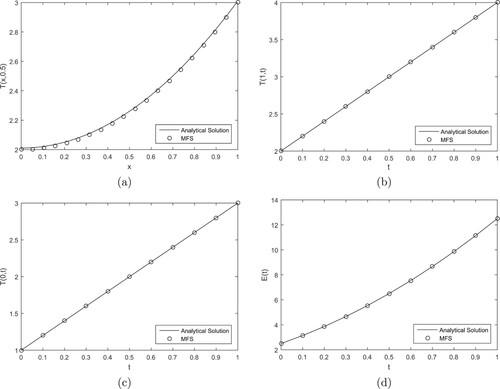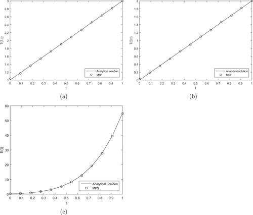4) ). Figure 1 compares the analytical solution for $T(x,0.5)=x^2+2$, $T(1,t)=2+2t$, $T(0,t)=2t+1$ and $E(t)=(T^2(0,t)+T^2(1,t))/2=(8t^2+12t+5)/2$ with the corresponding MFS numerical solutions obtained from (9(9) $\begin{array}{r}A(\underset{\_}{c})=\underset{\_}{r},\end{array}$(9) ). We can see that the MFS is very accurate in solving the direct problem.

Figure 1. The analytical and MFS numerical solutions for: (a) $T(x,0.5)$, (b) $T(1,t)$, (c) $T(0,t)$ and (d) $E(t)$, obtained when solving the direct problem for Example 1. Corresponding to the results for $T(x,0.5)$, $T(1,t)$, $T(0,t)$ and $E(t)$, the maximum pointwise relative errors between the analytical and numerical MFS solutions are $0.5\mathrm{\%}$, $0.2\mathrm{\%}$, $0.3\mathrm{\%}$ and $0.01\mathrm{\%}$, respectively.

Next, we investigate the inverse problem (1a(1a) $\begin{array}{r}\frac{\mathrm{\partial }T}{\mathrm{\partial }t}(x,t)=\frac{{\mathrm{\partial }}^{2}T}{\mathrm{\partial }{x}^2}(x,t),(x,t)\in (0,1)\times (0,t_f),\end{array}$(1a) )–(1d(1d) $\begin{array}{r}\frac{\mathrm{\partial }T}{\mathrm{\partial }x}(1,t)+\rho (t)g(T(1,t))=h_1(t),t\in [0,t_f),\end{array}$(1d) ) and (2(2) $\begin{array}{r}Y(t)=T(1,t),t\in [0,t_f),\end{array}$(2) ) and, in particular, we undertake an analysis of choosing the modelling parameter ${\sigma }_{\rho }$ in the random walk (15(15) $\begin{array}{rl}{\rho }_k& ={\rho }_{k-1}+{\sigma }_{\rho }{e}_k,k=1,\dots ,M,\end{array}$(15) ) for the HTC. Let us consider the additive error measurement (19(19) $\begin{array}{r}{Y}_a(t_k)=Y(t_k)+{ϵ}_k,k=1,\dots ,M,\end{array}$(19) ) with $p=1\mathrm{\%}$ noise. We have tested three different standard deviations ${\sigma }_{\rho }\in \{0.02,0.2,0.4\}$ for the random walk (15(15) $\begin{array}{rl}{\rho }_k& ={\rho }_{k-1}+{\sigma }_{\rho }{e}_k,k=1,\dots ,M,\end{array}$(15) ) related to the expected rate of change of the HTC. When sample impoverishment takes place, most of the particles are eliminated during the resampling step. Arulampalam et al. [16] suggested that if the effective sample size Neff is over $50\mathrm{\%}$ of $N_{\mathrm{part}}$ the degeneracy is not significant. We also follow the lines of [22] in which Neff was used as an indicator of the ”optimal” value for ${\sigma }_{\rho }$ in a heat transfer inverse problem concerned with the sequential estimation of an unknown heat flux from experimental measurements.

Table 1 shows the results of the evaluation criteria, in which Neff [$\mathrm{\%}$] denotes the average percentage relative error between the effective sample size and the total number of particles obtained by the particle filter. Note that ${\sigma }_{\rho }=0.02$ gives low values of Neff [$\mathrm{\%}$] and MWCI, and consequently inaccurate results because the evolution model (random walk) (15(15) $\begin{array}{rl}{\rho }_k& ={\rho }_{k-1}+{\sigma }_{\rho }{e}_k,k=1,\dots ,M,\end{array}$(15) ) for the HTC depends strongly on the prior information, i.e. the initial estimate of the particle filter. This is typical with particle filters that are essentially MCMC-type algorithms which have difficulties with small variances. Moreover, since the parameter space (or search field) of HTC was not fully explored, this causes the particle filter to have Neff [$\mathrm{\%}$] smaller than $50\mathrm{\%}$. It was noted that sample impoverishment is substantial, because in this situation the width of the credible interval is almost zero. When ${\sigma }_{\rho }$ was increased to 0.2 and then to 0.4, the filter performance improved without sample impoverishment. For illustration, Figure 2 shows the results obtained by the SIR filter with $N_{\mathrm{part}}=200$ and ${\sigma }_{\rho }\in \{0.2,0.4\}$. The filtered boundary temperature measurements (19(19) $\begin{array}{r}{Y}_a(t_k)=Y(t_k)+{ϵ}_k,k=1,\dots ,M,\end{array}$(19) ) contaminated with $p=1\mathrm{\%}$ noise are also included in Figures 2(c) and 2(d). Once the dynamic behaviour of the random walk model improves, the filter is able to draw particles close to the actual HTC with suitable performance. In the remainder of this section we take ${\sigma }_{\rho }=0.2$ in (15(15) $\begin{array}{rl}{\rho }_k& ={\rho }_{k-1}+{\sigma }_{\rho }{e}_k,k=1,\dots ,M,\end{array}$(15) ).

Figure 2. Estimated $\rho (t)$ and the filtered boundary temperature measurements (19(19) $\begin{array}{r}{Y}_a(t_k)=Y(t_k)+{ϵ}_k,k=1,\dots ,M,\end{array}$(19) ) contaminated with $p=1\mathrm{\%}$ noise, obtained using the particle filter with $N_{\mathrm{part}}=200$ particles for (a) and (c) ${\sigma }_{\rho }=0.2$; (b) and (d) ${\sigma }_{\rho }=0.4$, for Example 1.

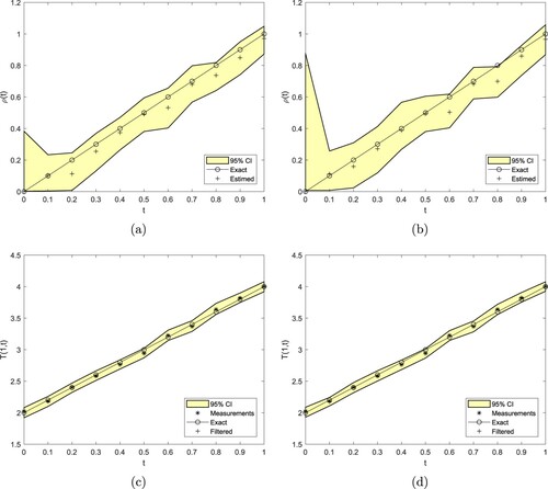
Table 1. Results for various ${\sigma }_{\rho }$ for $p=1\mathrm{\%}$ noise in Equation (19(19) $\begin{array}{r}{Y}_a(t_k)=Y(t_k)+{ϵ}_k,k=1,\dots ,M,\end{array}$(19) ) for Example 1.

$N_{\mathrm{part}}$	${\sigma }_{\rho }$	$RMS{E}_{\rho }$	$Rel(\rho )\mathrm{\%}$	MWCI	Neff [$\mathrm{\%}$]
50	0.02	0.460	77.8	0.04	2.00
100	0.02	0.460	77.7	0.07	2.15
200	0.02	0.405	68.5	0.06	2.26
50	0.2	0.049	8.36	0.25	64.20
100	0.2	0.047	8.00	0.29	67.36
200	0.2	0.045	7.22	0.25	64.80
50	0.4	0.053	9.11	0.28	50.05
100	0.4	0.051	8.68	0.29	50.70
200	0.4	0.047	8.10	0.29	52.31

Table 2 presents the results of the evaluation criteria obtained by the particle filter for $p=5\mathrm{\%}$ noise in Equation (19(19) $\begin{array}{r}{Y}_a(t_k)=Y(t_k)+{ϵ}_k,k=1,\dots ,M,\end{array}$(19) ). It is worth remarking that there was no sample impoverishment as Neff [$\mathrm{\%}$] was always greater than $50\mathrm{\%}$.

Table 2. Results for $p=5\mathrm{\%}$ noise in Equation (19(19) $\begin{array}{r}{Y}_a(t_k)=Y(t_k)+{ϵ}_k,k=1,\dots ,M,\end{array}$(19) ) with ${\sigma }_{\rho }=0.2$ for Example 1.

$N_{\mathrm{part}}$	$RMS{E}_{\rho }$	$Rel(\rho )\mathrm{\%}$	MWCI	Neff [$\mathrm{\%}$]
50	0.118	19.93	0.67	77.53
100	0.110	18.72	0.59	73.82
200	0.109	18.57	0.55	75.29

Previously, Yan et al. [32], using a Bayesian MCMC inference approach, obtained the relative errors Rel(ρ) $\in \{3.84,8.07\}\mathrm{\%}$ for $p\in \{1,5\}\mathrm{\%}$ noise in Equation (19(19) $\begin{array}{r}{Y}_a(t_k)=Y(t_k)+{ϵ}_k,k=1,\dots ,M,\end{array}$(19) ), respectively. On the other hand, see Tables 1 and 2 for ${\sigma }_{\rho }=0.2$ and $N_{\mathrm{part}}=200$, our SIR filter results give larger relative errors of Rel(ρ) $\in \{7.22,18.57\}\mathrm{\%}$ for $p\in \{1,5\}\mathrm{\%}$ noise in Equation (19(19) $\begin{array}{r}{Y}_a(t_k)=Y(t_k)+{ϵ}_k,k=1,\dots ,M,\end{array}$(19) ), respectively. However, the MCMC method of [32], which used all the time history measurements (2(2) $\begin{array}{r}Y(t)=T(1,t),t\in [0,t_f),\end{array}$(2) ) or (3(3) $\begin{array}{r}E(t)={\int }_{\mathrm{\partial }\mathrm{\Omega }}\mathrm{\Phi }(T(x,t))\mathrm{d}s(x)=\mathrm{\Phi }(T(0,t))+\mathrm{\Phi }(T(1,t)),t\in [0,t_f),\end{array}$(3) ) globally, it has also resulted in some negative values for the HTC which are physically unrealistic. The same happened with the results of [49], obtained using the boundary element method (BEM), with no positivity constraint or regularization imposed. However, neither negativity nor instability happened with the particle filter which uses one measurement at a time in a sequential manner. Therefore, eventhough the SIR filter has yielded results with a relative error twice as larger than the MCMC method, it has demonstrated reasonably accurate and stable results without unphysical negative estimates for the HTC. With reduced information, the credible interval has comparable width to the results of [11] and in addition, the CPU time is relatively small.

The results in Tables 1 and 2 have been obtained for the boundary temperature measurement (2(2) $\begin{array}{r}Y(t)=T(1,t),t\in [0,t_f),\end{array}$(2) ) contaminated with additive noise (19(19) $\begin{array}{r}{Y}_a(t_k)=Y(t_k)+{ϵ}_k,k=1,\dots ,M,\end{array}$(19) ). In Table 3 we present the results of the evaluation criteria obtained using the particle filter for solving the inverse problem (1a(1a) $\begin{array}{r}\frac{\mathrm{\partial }T}{\mathrm{\partial }t}(x,t)=\frac{{\mathrm{\partial }}^{2}T}{\mathrm{\partial }{x}^2}(x,t),(x,t)\in (0,1)\times (0,t_f),\end{array}$(1a) )–(1d(1d) $\begin{array}{r}\frac{\mathrm{\partial }T}{\mathrm{\partial }x}(1,t)+\rho (t)g(T(1,t))=h_1(t),t\in [0,t_f),\end{array}$(1d) ) with the non-standard measurement (3(3) $\begin{array}{r}E(t)={\int }_{\mathrm{\partial }\mathrm{\Omega }}\mathrm{\Phi }(T(x,t))\mathrm{d}s(x)=\mathrm{\Phi }(T(0,t))+\mathrm{\Phi }(T(1,t)),t\in [0,t_f),\end{array}$(3) ) given by $E(t)=(8t^2+12t+5)/2$, contaminated with additive noise (20(20) $\begin{array}{r}{E}_a(t_k)=E(t_k)+{ϵ}_k,k=1,\dots ,M,\end{array}$(20) ). This is a benchmark test example, already considered in [33] with the analytical solution given by Equations (23(23) $\begin{array}{r}T(x,t)=x^2+2t+1\end{array}$(23) ) and (24(24) $\begin{array}{r}\rho (t)=t.\end{array}$(24) ), and is investigated here for comparison purposes.

Table 3. Results for $p\in \{1,5\}\mathrm{\%}$ noise in Equation (20(20) $\begin{array}{r}{E}_a(t_k)=E(t_k)+{ϵ}_k,k=1,\dots ,M,\end{array}$(20) ) with ${\sigma }_{\rho }=0.2$ for Example 1.

$N_{\mathrm{part}}$	p	$RMS{E}_{\rho }$	$Rel(\rho )\mathrm{\%}$	MWCI	Neff [$\mathrm{\%}$]
50	$1\mathrm{\%}$	0.0502	8.48	0.27	85.67
100	$1\mathrm{\%}$	0.045	7.73	0.27	85.56
200	$1\mathrm{\%}$	0.041	7.07	0.23	84.69
50	$5\mathrm{\%}$	0.074	12.54	0.65	58.43
100	$5\mathrm{\%}$	0.071	12.10	0.56	63.85
200	$5\mathrm{\%}$	0.057	9.65	0.59	61.17

Figures 2(a), 3(a) and 4(a), 4(b) show the estimated HTC $\rho (t)$ from the particle filter algorithm with ${\sigma }_{\rho }=0.2$ and $N_{\mathrm{part}}=200$ particles applied to the inversion of the data (19(19) $\begin{array}{r}{Y}_a(t_k)=Y(t_k)+{ϵ}_k,k=1,\dots ,M,\end{array}$(19) ), (20(20) $\begin{array}{r}{E}_a(t_k)=E(t_k)+{ϵ}_k,k=1,\dots ,M,\end{array}$(20) ) contaminated with $p=1\mathrm{\%}$ and $p=5\mathrm{\%}$ additive noise, respectively. The corresponding filtered data are plotted in Figures 2(c), 3(c) and 4(c), 4(d), respectively. In all Figures 2–4, the credible intervals have been included.

Figure 3. Estimated $\rho (t)$ and the filtered measurements (20(20) $\begin{array}{r}{E}_a(t_k)=E(t_k)+{ϵ}_k,k=1,\dots ,M,\end{array}$(20) ) contaminated with $p=1\mathrm{\%}$ noise, obtained using the particle filter with ${\sigma }_{\rho }=0.2$ and $N_{\mathrm{part}}=200$ particles, for Example 1.

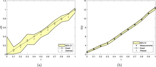
Figure 4. Estimated $\rho (t)$ from the measurements (a) (19(19) $\begin{array}{r}{Y}_a(t_k)=Y(t_k)+{ϵ}_k,k=1,\dots ,M,\end{array}$(19) ) or (b) (20(20) $\begin{array}{r}{E}_a(t_k)=E(t_k)+{ϵ}_k,k=1,\dots ,M,\end{array}$(20) ) contaminated with $p=5\mathrm{\%}$ noise, as filtered in (c) and (d), respectively, obtained using the particle filter with ${\sigma }_{\rho }=0.2$ and $N_{\mathrm{part}}=200$ particles, for Example 1.

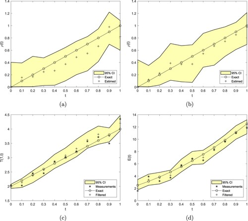
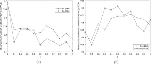
Figure 5(a ,b) show the variation of the MWCI for the SIR filter, comparing the results obtained for $p=1\mathrm{\%}$ and $p=5\mathrm{\%}$ noise in the measurement (19(19) $\begin{array}{r}{Y}_a(t_k)=Y(t_k)+{ϵ}_k,k=1,\dots ,M,\end{array}$(19) ) or (20(20) $\begin{array}{r}{E}_a(t_k)=E(t_k)+{ϵ}_k,k=1,\dots ,M,\end{array}$(20) ). All results presented in Figures 2–5 demonstrate that as the measured data becomes more accurate, i.e. as p decreases from $5\mathrm{\%}$ to $1\mathrm{\%}$, the MWCI decreases. They also indicate that measuring the non-standard quantity (3(3) $\begin{array}{r}E(t)={\int }_{\mathrm{\partial }\mathrm{\Omega }}\mathrm{\Phi }(T(x,t))\mathrm{d}s(x)=\mathrm{\Phi }(T(0,t))+\mathrm{\Phi }(T(1,t)),t\in [0,t_f),\end{array}$(3) ) contains more information in the inverse problem than the standard boundary temperature measurement (2(2) $\begin{array}{r}Y(t)=T(1,t),t\in [0,t_f),\end{array}$(2) ), as the results obtained show smaller width of credible intervals.

Figure 5. The variation of the MWCI over time for (a) $p=1\mathrm{\%}$ and (b) $p=5\mathrm{\%}$ noise in Equation (19(19) $\begin{array}{r}{Y}_a(t_k)=Y(t_k)+{ϵ}_k,k=1,\dots ,M,\end{array}$(19) ) or Equation (20(20) $\begin{array}{r}{E}_a(t_k)=E(t_k)+{ϵ}_k,k=1,\dots ,M,\end{array}$(20) ), obtained using the particle filter with ${\sigma }_{\rho }=0.2$ and $N_{\mathrm{part}}=200$ particles, for Example 1.

5.2. Example 2

In the second example given by Equations (1a(1a) $\begin{array}{r}\frac{\mathrm{\partial }T}{\mathrm{\partial }t}(x,t)=\frac{{\mathrm{\partial }}^{2}T}{\mathrm{\partial }{x}^2}(x,t),(x,t)\in (0,1)\times (0,t_f),\end{array}$(1a) )–(1d(1d) $\begin{array}{r}\frac{\mathrm{\partial }T}{\mathrm{\partial }x}(1,t)+\rho (t)g(T(1,t))=h_1(t),t\in [0,t_f),\end{array}$(1d) ) and (3(3) $\begin{array}{r}E(t)={\int }_{\mathrm{\partial }\mathrm{\Omega }}\mathrm{\Phi }(T(x,t))\mathrm{d}s(x)=\mathrm{\Phi }(T(0,t))+\mathrm{\Phi }(T(1,t)),t\in [0,t_f),\end{array}$(3) ), and considered before in [26], we take $t_f=1$ and $T^0(x)=x^2$, $h_0(t)=16t^4(t+1)$, $h_1(t)=(1+t)(1+2t{)}^4+2$, $\rho (t)=1+t$, $g(T)=T^3|T|$ corresponding to nonlinear radiation, and the measurements (3(3) $\begin{array}{r}E(t)={\int }_{\mathrm{\partial }\mathrm{\Omega }}\mathrm{\Phi }(T(x,t))\mathrm{d}s(x)=\mathrm{\Phi }(T(0,t))+\mathrm{\Phi }(T(1,t)),t\in [0,t_f),\end{array}$(3) ) given by $E(t)=12.8t^5+16t^4+8t^2+2t+0.2$. In this example, the direct problem has the analytical solution (25) $\begin{array}{r}T(x,t)=x^2+2t.\end{array}$(25) We apply the MFS with M = 12, N = M−2 = 10 and the source points uniformly located on $y_0=-1$, $y_1=2$, i.e. h = 1. The MFS nonlinear system (9(9) $\begin{array}{r}A(\underset{\_}{c})=\underset{\_}{r},\end{array}$(9) ) is solved using the fsolve MATLAB function routine, which uses the Levenberg-Marquardt method.

First, for the direct problem, Figure 6 shows the MFS solution compared to the analytical solution for $T(1,t)$, $T(0,t)$ and $E(T)$, and accurate numerical results can be observed. The errors are higher than those in Figure 1 for Example 1 because in Example 2 the direct problem is nonlinear due to the nonlinearity of the HTC in the in the boundary conditions (1c(1c) $\begin{array}{r}-\frac{\mathrm{\partial }T}{\mathrm{\partial }x}(0,t)+\rho (t)g(T(0,t))=h_0(t),t\in [0,t_f),\end{array}$(1c) ) and (1d(1d) $\begin{array}{r}\frac{\mathrm{\partial }T}{\mathrm{\partial }x}(1,t)+\rho (t)g(T(1,t))=h_1(t),t\in [0,t_f),\end{array}$(1d) ).

Figure 6. The analytical and MFS numerical solutions for: (a) $T(1,t)$, (b) $T(0,t)$, (c) $E(t)$, obtained when solving the direct problem for Example 2. Corresponding to the results for $T(1,t)$, $T(0,t)$ and $E(t)$, the maximum pointwise relative errors between the analytical and numerical MFS solutions are $4\mathrm{\%}$, $2\mathrm{\%}$ and $0.2\mathrm{\%}$, respectively.

Next, we present in Table 4 and Figure 7 the numerical results obtained by inverting the data (3(3) $\begin{array}{r}E(t)={\int }_{\mathrm{\partial }\mathrm{\Omega }}\mathrm{\Phi }(T(x,t))\mathrm{d}s(x)=\mathrm{\Phi }(T(0,t))+\mathrm{\Phi }(T(1,t)),t\in [0,t_f),\end{array}$(3) ) contaminated with $p\in \{1\mathrm{\%},5\mathrm{\%}\}$ additive noise (20(20) $\begin{array}{r}{E}_a(t_k)=E(t_k)+{ϵ}_k,k=1,\dots ,M,\end{array}$(20) ). Compared to Table 3 of Example 1, it can be observed that the results of Table 4 reveal higher MWCI and lower Neff. Moreover, it can be seen that the evaluation error criteria are consistent with the errors in the data and the estimated HTC lies within a credible interval of reasonable width. Furthermore, the results illustrated in Figure 7(b) reveal comparable accuracy with the numerical results presented in Figure 2(e) of [26] obtained without regularization.

Figure 7. (a) Estimated $\rho (t)$ from the measurements (20(20) $\begin{array}{r}{E}_a(t_k)=E(t_k)+{ϵ}_k,k=1,\dots ,M,\end{array}$(20) ) with (a) $p=1\mathrm{\%}$ and (b) $p=5\mathrm{\%}$ noise, as filtered in (c) and (d), respectively, along with (e) the variation of the MWCI over time, obtained using the particle filter with ${\sigma }_{\rho }=0.2$ and $N_{\mathrm{part}}=200$ particles, for Example 2.

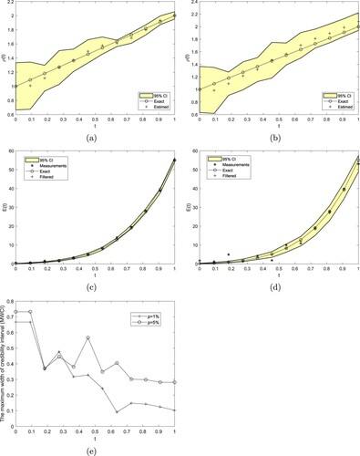
Table 4. Results for $p\in \{1,5\}\mathrm{\%}$ noise in Equation (20(20) $\begin{array}{r}{E}_a(t_k)=E(t_k)+{ϵ}_k,k=1,\dots ,M,\end{array}$(20) ) with ${\sigma }_{\rho }=0.2$ for Example 2.

$N_{\mathrm{part}}$	p	$RMS{E}_{\rho }$	$Rel(\rho )\mathrm{\%}$	MWCI	Neff [$\mathrm{\%}$]
50	$1\mathrm{\%}$	0.068	4.46	0.67	63.26
100	$1\mathrm{\%}$	0.060	3.96	0.71	64.29
200	$1\mathrm{\%}$	0.056	3.66	0.70	64.64
50	$5\mathrm{\%}$	0.220	14.37	0.72	53.06
100	$5\mathrm{\%}$	0.203	13.26	0.82	54.80
200	$5\mathrm{\%}$	0.176	11.49	0.79	55.20

6. Conclusions

The MFS has become an important tool for the numerical solution of inverse problems [1]. In this paper, we have combined the SIR particle filter algorithm and the MFS to estimate the time-dependent HTC in inverse heat conduction problems. The governing boundary condition of the third kind may be of a linear convective or nonlinear radiative Robin type. For a unique solution, extra information was given by the temperature specification at one boundary point or the non-local boundary integral observation (3(3) $\begin{array}{r}E(t)={\int }_{\mathrm{\partial }\mathrm{\Omega }}\mathrm{\Phi }(T(x,t))\mathrm{d}s(x)=\mathrm{\Phi }(T(0,t))+\mathrm{\Phi }(T(1,t)),t\in [0,t_f),\end{array}$(3) ). Compared to the numerical results produced by other methods, the MFS+SIR has yielded comparable results in terms of accuracy, stability and width of the credible intervals, with additional improved features such as CPU time efficiency and preservation of the physical non-negativity of the HTC. These improvements have been illustrated on smooth test examples with analytical solutions available. This way the input data (2(2) $\begin{array}{r}Y(t)=T(1,t),t\in [0,t_f),\end{array}$(2) ) and (3(3) $\begin{array}{r}E(t)={\int }_{\mathrm{\partial }\mathrm{\Omega }}\mathrm{\Phi }(T(x,t))\mathrm{d}s(x)=\mathrm{\Phi }(T(0,t))+\mathrm{\Phi }(T(1,t)),t\in [0,t_f),\end{array}$(3) ) for the inverse problem has been generated directly from the temperature expressions (23(23) $\begin{array}{r}T(x,t)=x^2+2t+1\end{array}$(23) ) and (25(25) $\begin{array}{r}T(x,t)=x^2+2t.\end{array}$(25) ) such that no inverse crime has been committed. On the other hand, retrieving more severe HTCs presenting discontinuities may represent currently a limitation of the MFS requiring further consideration in the future.

Acknowledgments

The hospitality of the University of Leeds while the first author was visiting there is gratefully acknowledged. The comments and suggestions made by the referees are also gratefully acknowledged.

Disclosure statement

No potential conflict of interest was reported by the author(s).

Additional information

Funding

The Brazilian authors acknowledge the financial support provided by the Brazilian sponsoring agencies Conselho Nacional de Desenvolvimento Científico e Tecnológico (CNPq) and Fundação de Amparo à Pesquisa e Inovação do Espìrito Santo (FAPES).

References

- Karageorghis A, Lesnic D, Marin L. A survey of applications of the MFS to inverse problems. Inverse Probl Sci Eng. 2011;19:309–336.
- Karageorghis A, Fairweather G. The method of fundamental solutions for the numerical solution of the biharmonic equation. J Comput Phys. 1987;69:434–459.
- Bogomolny A. Fundamental solutions method for elliptic boundary value problems. SIAM J Numer Anal. 1985;22:644–669.
- Alves CJS, Chen CS. A new method of fundamental solutions applied to nonhomogeneous elliptic problems. Adv Comput Math. 2005;23:125–142.
- Kupradze VD, Aleksidze MA. The method of functional equations for the approximate solution of certain boundary value problems. USSR Comput Math Math Phys. 1964;4:82–126.
- Johansson BT, Lesnic D. A method of fundamental solutions for transient heat conduction. Eng Anal Bound Elem. 2008;32:697–703.
- Johansson BT, Lesnic D, Reeve T. A comparative study on applying the method of fundamental solutions to the backward heat conduction problem. Math Comput Model. 2011;54(1-2):403–416.
- Johansson BT, Lesnic D, Reeve T. The method of fundamental solutions for the two-dimensional inverse Stefan problem. Inverse Probl Sci Eng. 2014;22(1):112–129.
- Dawson M, Borman D, Hammond RB, et al. A meshless method for solving a two-dimensional transient inverse geometric problem. Int J Numer Methods Heat Fluid Flow. 2013;23(5):790–817.
- Masson PL, Loulou T, Artioukhine E. Estimation of a 2D convection heat transfer coefficient during a test: comparison between two methods and experimental validation. Inverse Probl Sci Eng. 2004;12:594–617.
- Yang F, Yan L, Wei T. The identification of a Robin coefficient by a conjugate gradient method. Int J Numer Methods Eng. 2009;78:800–816.
- Kaipio J, Somersalo E. Statistical and computational inverse problems. Berlin: Springer-Verlag; 2004.
- Winkler R. An introduction to Bayesian inference and decision. Gainsville (FL): Probabilistic Publishing; 2003.
- Doucet A, Godsill S, Andrieu C. On sequential Monte Carlo sampling methods for Bayesian filtering. Stat Comput. 2000;10:197–208.
- Kalman R. A new approach to linear filtering and prediction problems. ASME J Basic Eng. 1960;82:35–45.
- Arulampalam S, Maskell S, Gordon N, et al. A tutorial on particle filters for on-line non-linear/non-Gaussian Bayesian tracking. IEEE Trans Signal Process. 2001;50:174–188.
- Kaipio J, Duncan S, Seppanen A, et al. Handbook of process imaging for automatic control, state estimation for process imaging. Boca Raton (FL): CRC Press; 2005.
- Andrieu C, Doucet A, Sumeetpal S, et al. Particle methods for charge detection, system identification and control. Proc IEEE. 2004;92:423–438.
- Hammersley JM, Hanscomb DC. Monte Carlo methods. New York: Chapman and Hall; 1964.
- Gordon N, Salmond D, Smith AFM. Novel approach to nonlinear and non-Gaussian Bayesian state estimation. Inst Electr Eng. 1993;140:107–113.
- Orlande HRB, Colaço MJ, Dulikravich GS, et al. State estimation problems in heat transfer. Int J Uncertain Quantif. 2012;2:239–258.
- Silva WB, Dutra JCS, Costa JMJ, et al. A hybrid estimation scheme based on the sequential importance resampling particle filter and the particle swarm optimization (PSO-SIR). In: Computational intelligence, optimization and inverse problems with applications in engineering. New York: Springer International Publishing; 2019. p. 247–261.
- Louahlia-Gualous H, Panday PK, Artioukhine EA. Inverse determination of the local heat transfer coefficients for nucleate boiling on a horizontal cylinder. J Heat Transf. 2003;125:1087–1095.
- Osman AM, Beck JV. Investigation of transient heat transfer coefficients in quenching experiments. J Heat Transf. 1990;112:843–848.
- Slodicka M, Van Keer R. Determination of a Robin coefficient in semilinear parabolic problems by means of boundary measurements. Inverse Probl. 2002;18:139–152.
- Slodička M, Lesnic D, Onyango TTM. Determination of a time-dependent heat transfer coefficient in a nonlinear inverse heat conduction problem. Inverse Probl Sci Eng. 2010;18:65–81.
- Johansson BT, Lesnic D, Reeve T. A method of fundamental solutions for two-dimensional heat conduction. Int J Comput Math. 2011;88(8):1697–1713.
- da Silva WB, Dutra JCS, Kepperschimidt CEP, et al. Sequential particle filter estimation of a time-dependent heat transfer coefficient in a multidimensional nonlinear inverse heat conduction problem. Appl Math Model. 2021;89:654–668.
- Lesnic D, Elliott L, Ingham DB. A boundary element method for the determination of the transmissivity of a heterogeneous aquifer in groundwater flow systems. Eng Anal Bound Elem. 1998;21(3):223–234.
- Johansson BT, Lesnic D. A method of fundamental solutions for transient heat conduction in layered materials. Eng Anal Bound Elem. 2009;33(12):1362–1367.
- Friedman A. Partial differential equations of parabolic type. Englewood Cliffs (NJ): Prentice Hall; 1964.
- Yan L, Yang F, Fu C. Bayesian inference approach to identify a Robin coefficient in one-dimensional parabolic problems. J Comput Appl Math. 2009;231:840–850.
- Onyango TTM, Ingham DB, Lesnic D, et al. Determination of a time-dependent heat transfer coefficient non-standard boundary measurements. Math Comput Simul. 2009;79:1577–1584.
- Su J, Hewitt GF. Inverse heat conduction problem of estimating time-varying heat transfer coefficient. Numer Heat Transf Part A. 2004;45:777–789.
- Nho Hao Dinh, Viet Huong Bui, Xuan Thanh Phan, et al. Identification of nonlinear heat transfer laws from boundary observations. Appl Anal. 2015;94:1784–1799.
- Aykroyd RG, Lesnic D, Karageorghis A. A fully Bayesian approach to shape estimation of objects from tomography data using MFS forward solutions. Int J Tomogr Simul. 2015;28:1–21.
- Grabski JK. On the sources placement in the method of fundamental solutions for time-dependent heat conduction problems. Comput Math Appl. 2021;88:33–51.
- Johansson BT. Properties of a method of fundamental solutions for the parabolic heat equation. Appl Math Lett. 2017;65:83–89.
- Campillo F, Rossi V. Convolution particle filter for parameter estimation in general state-space models. IEEE Trans Aerosp Electron Syst. 2009;45:1073–1072.
- Doucet A, Freitas N, Gordon N. Sequential Monte Carlo methods in practice. Berlin: Springer; 2001.
- Doucet A, Tadic VB. Parameter estimation in general state–space models using particle methods. Ann Inst Stat Math. 2003;55:409–422.
- Liu J, West M. Combined parameter and state estimation in simulation-based filtering. In: Sequential Monte Carlo methods in practice. Statistics for Engineering and Information Science. New York: Springer; 2001. p. 197–223.
- Silva WB, Rochoux MC, Orlande HRB, et al. Application of particle filters to regional-scale wildfire spread. High Temperatures High Pressures. 2014;43:415–440.
- Salardani LSF, Albuquerque LP, Costa JMJ, et al. Particle filter-based monitoring scheme for simulated bio-ethylene production process. Inverse Probl Sci Eng. 2018;27:648–668.
- Ristic B, Arulampalam S, Gordon N. Beyond the Kalman filter. Boston: Artech House; 2004.
- Dias ACSR, Da Silva WB, Dutra JCS. Propylene polymerization reactor control and estimation using a particle filter and neural network. Macromol React Eng. 2017;11:1–20.
- Marques R, Silva WB, Hoffmann R, et al. Sequential state inference of engineering systems through the particle move-reweighting algorithm. Comput Appl Math. 2017;37:220–236.
- Liu J, Chen R. Sequential Monte Carlo methods for dynamical systems. J Amer Statist Assoc. 1998;93:1032–1044.
- Onyango TTM, Ingham DB, Lesnic D. Reconstruction of heat transfer coefficients using the boundary element method. Comput Math Appl. 2008;56(1):114–126.