Identification of deformable droplets from boundary measurements: the case of non-stationary Stokes problem

Abstract

In this paper, we use asymptotic expansion of the velocity field to reconstruct small deformable droplets (i.e. their forms and locations) immersed in an incompressible Newtonian fluid. Here the fluid motion is assumed to be governed by the non-stationary linear Stokes system. Taking advantage of the smallness of the droplets, our asymptotic formula and identification methods extend those already derived for rigid inhomogeneity and for stationary Stokes system. Our derivations, based on dynamical boundary measurements, are rigorous and proved by involving the notion of viscous moment tensor VMT. The viability of our reconstruction approach is documented by numerical results.

Keywords:

• Non-stationary Stokes system
• asymptotic expansion
• viscous moment tensor
• deformable droplet

2010 Mathematics Subject Classifications:

• 35R30
• 35Q30
• 35B30
• 76D55

1. Introduction

In this paper, we derive an asymptotic expansion of a weighted boundary measurements, expressed in term of velocity field, in the presence of multiple small deformable droplets (modelled by deformable inhomogeneities) immersed in an incompressible Newtonian fluid. This asymptotic expansion, through a convenable application system, will allow us to identify these droplets having kinematic viscosities different from the background medium. The system is modeled as a non-stationary Stokes flow, in an open bounded domain $\mathrm{\Omega }\subset {\mathbb{R}}^d$ that contains deformable inhomogeneities (droplets) of small size, say α. The non-stationary Stokes equations are a standard system of PDE's governing the flow of continuum matter in fluid form, such as liquid or gas, occupying the domain Ω. These equations describe the change with respect to time $t\in [0,T]$ of the velocity and pressure of the fluid.

The detection and the reconstruction of an object immersed in a fluid is a source of many investigations [1–7]. This kind of inverse problems arises, for example, in moulds filling during which small gas bubbles can be created and trapped inside the material (as it is mentioned in [5,7]) or in the detection of mines.

In this paper, we consider a dilute suspension of deformable droplets in a matrix fluid. We assume that the droplets and matrix fluid to be Newtonian and neglect inertia and body forces. As it is mentioned in [6], the evolution of droplet shape only depends on the viscosity difference between the fluids and on surface tension. Then, we make the assumption of small size of these inhomogeneities to use asymptotic formula which allows us to solve a given inverse problem. This assumption was used before, for different kinds of problems, in [3,7–11] and in others. We further assume that the small droplets are at a distance $\gg \alpha$ away from each other, and are also away from the boundary, to be able to neglect droplet interactions and their interaction with the boundary $\mathrm{\partial }\mathrm{\Omega }$.

The goal of this work is to expand, in a mathematically rigorous way, a numerical approach to identify the locations of the droplets from boundary measurements of the velocity field. We get an asymptotic expansion of solutions to the transmission problem for the non-stationary Stokes equations in terms of the geometry of the droplets. This procedure describes the perturbation of the solution caused by the presence of deformable obstacles with small diameters. Based on this results, we derive an asymptotic expansion for a weighted boundary measurements ${\mathrm{\Lambda }}_{\alpha }\left(T\right)$ (as $\alpha \to 0$) in terms of viscous moment tensor VMT. This is partially inspired from the general idea developed, for a heat equation, in [8] to locate multiple inclusions and from the fact that the Stokes system can be viewed as the incompressible limit (the compression modulus is infinite) [3].

The formula that is developed is considerably different from the topological sensitivity analysis method and allows us to find the locations of the inhomogeneities with significant accuracy. It is explicit and can be easily performed numerically. The results and the general approach that we will adopt here extend more those for rigid inclusions [2,4,5,12–14] and for stationary stokes cases [3,6,7,11,15] among others. However, they remain a little close to the common ideas of that developed for reconstructing small conductivity inclusions from boundary measurements, see [9,10,12,16,17] and the references therein. In addition, readers are recommended to consult important works on other types of inverse problems [18–21], and do not forget that we can refer to the books (for example, [22–24]) to get acquainted with the main notations, the calculation techniques and the most well-known theorems used naturally for Stokes system.

The paper is organized as follows. In the next section, we formulate our model problem for droplets in a non-stationary Stokes flow. We state our main results in Section 3. The rigorous derivation of the asymptotic expansion, for the pattern ${\mathrm{\Lambda }}_{\alpha }\left(T\right)$, is detailed in Section 4 in terms of the notion of viscous moment tensor VMT. In Section 5, we use our asymptotic expansion to make up a reconstruction method by introducing a so-called identifier of interest which, by some T>0, recover the discrete locations $z_j;j=1,\dots ,m$ of the droplets. We then perform numerical experiments to test the viability of the method.

2. Problem formulation

Let Ω be a bounded, open connected subdomain of ${\mathbb{R}}^d$, d = 2, 3 with $C^{1,1}$- boundary $\mathrm{\partial }\mathrm{\Omega }$. Let ν denote the outward unit normal to $\mathrm{\partial }\mathrm{\Omega }$. We suppose that Ω contains a finite number of droplets, each of the form $z_j+\alpha B_j$, where $B_j\subset {\mathbb{R}}^d$ is a bounded, smooth domain containing the origin. The total collection of deformable inhomogeneities thus takes the form ${\displaystyle {\mathcal{B}}_{\alpha }={\displaystyle {\cup }_{j=1}^m(z_j+\alpha B_j)}}$. The points $z_j\in \mathrm{\Omega },j=1,\dots ,m,$ that determine the location of the droplets are assumed to satisfy (1) $|z_j-z_l|\ge d_0>0,\mathrm{\forall }j\ne l\text{ and }\text{ dist}(z_j,\mathrm{\partial }\mathrm{\Omega })\ge d_0>0.$(1) We also assume that $\alpha >0$, the common order of magnitude of the diameters of the inhomogeneities, is sufficiently small that these are disjoint and their distance to ${\mathbb{R}}^d\setminus \overline{\mathrm{\Omega }}$ is large than $d_0/2$. Let ${\mu }_0$ denote the viscosity of the background medium, for simplicity we shall assume in this paper that it is constant. Let ${\mu }_j$ denote the constant viscosity of the jth inhomogeneity $z_j+\alpha B_j$. Using this notation, we introduce the piecewise constant kinematic viscosity ${\mu }_{\alpha }\left(x\right)=\{\begin{array}{l}{\mu }_{0}x\in \mathrm{\Omega }\setminus \overline{{\mathcal{B}}_{\alpha }},\\ {\mu }_{j}x\in z_j+\alpha B_j,j=1,\dots ,m.\end{array}$ Before formulating the model problem in the presence of droplets and via a non-stationary Stokes flow, we introduce the following notations.

Notation: $I_d$ denotes the unit matrix in ${\mathbb{R}}^{d\times d}$, and $\mathbf{I}$ denotes the identity fourth-order tensor. The scalar product on ${\mathbb{R}}^{d\times d}$ is defined by $A:B=trace\left(A^{\mathrm{t}\mathrm{r}}B\right)$ where the superscript tr denotes the transpose of a matrix. $L_0^2\left(\mathrm{\Omega }\right)$ denotes the space of the functions of $L^2\left(\mathrm{\Omega }\right)$ which differ by a constant and throughout this paper, the inner product between two vectors u and w is denoted by $u\cdot w$. The strain rate tensor $\mathbf{e}$ for the flow is defined as follows: (2) $\mathbf{e}\left(u\right):=\frac{1}{2}(\mathrm{\nabla }u+(\mathrm{\nabla }u{)}^{\mathrm{t}\mathrm{r}})={\left(\frac{1}{2}(\frac{\mathrm{\partial }{u}_k}{\mathrm{\partial }{x}_l}+\frac{\mathrm{\partial }{u}_l}{\mathrm{\partial }{x}_k})\right)}_{1\le k,l\le d};u=(u_1,\dots ,u_d)\in {\mathbb{R}}^d.$(2) The divergence of a matrix-valued function A is denoted $\mathrm{D}\mathrm{i}\mathrm{v}\left(A\right)$, while the divergence of a vector-valued function u is denoted $\mathrm{d}\mathrm{i}\mathrm{v}\left(u\right)$. From now we denote by $L^2(\mathrm{\Omega }{)}^d$ the space of vector-valued functions whose components of its elements belong to the space $L^2\left(\mathrm{\Omega }\right)$ of square integrable functions. Likewise, we denote by $H^s(\mathrm{\Omega }{)}^d$ the space of vector-valued functions where the notation $H^s$ is used to denote those functions who along with all their derivatives of order less than or equal to s are in $L^2\left(\mathrm{\Omega }\right)$. We denote by $H^s(\mathrm{\partial }\mathrm{\Omega }{)}^d$ the trace space.

Let $(v_{\alpha },p_{\alpha })\in L^2(0,T;H^1(\mathrm{\Omega }{)}^d)\times L^2(0,T;H^1\left(\mathrm{\Omega }\right))$ be the solution to the following non-stationary linearized Navier–Stokes system: (3) $\{\begin{array}{l}{\displaystyle \frac{\mathrm{\partial }{v}_{\alpha }}{\mathrm{\partial }t}-\mathrm{D}\mathrm{i}\mathrm{v}(2{\mu }_{\alpha }\mathbf{e}\left(v_{\alpha }\right))+\mathrm{\nabla }{p}_{\alpha }=0\mathrm{i}\mathrm{n}\mathrm{\Omega }\times (0,T),}\\ \mathrm{d}\mathrm{i}\mathrm{v}\left(v_{\alpha }\right)=0\mathrm{i}\mathrm{n}\mathrm{\Omega },\\ v_{\alpha }{|}_{t=0}=\phi \mathrm{i}\mathrm{n}\mathrm{\Omega },\\ v_{\alpha }=g\mathrm{o}\mathrm{n}\mathrm{\partial }\mathrm{\Omega }\times (0,T).\end{array}$(3) Here T>0 is a final observation time, the initial condition $\phi \in {\mathcal{C}}^{\mathrm{\infty }}(\overline{\mathrm{\Omega }}{)}^d$ and, $g\in L^2(0,T;H^{1/2}(\mathrm{\partial }\mathrm{\Omega }{)}^d)$ is a non-homogeneous Dirichlet boundary data satisfying the standard flux compatibility condition: (4) ${\displaystyle {\int }_{\mathrm{\partial }\mathrm{\Omega }}g(x,t)\cdot \nu \mathrm{d}s\left(x\right)=0,a.e.t\in (0,T).}$(4)

We denote by $(v,p)\in L^2(0,T;H^1(\mathrm{\Omega }{)}^d)\times L^2(0,T;H^1\left(\mathrm{\Omega }\right))$ the solution of the non-stationary incompressible Stokes problem in the absence of any deformable inhomogeneities (the background solution): (5) $\{\begin{array}{l}{\displaystyle \frac{\mathrm{\partial }v}{\mathrm{\partial }t}-\mathrm{D}\mathrm{i}\mathrm{v}(2{\mu }_0\mathbf{e}\left(v\right))+\mathrm{\nabla }p=0\mathrm{i}\mathrm{n}\mathrm{\Omega }\times (0,T),}\\ \mathrm{d}\mathrm{i}\mathrm{v}\left(v\right)=0\mathrm{i}\mathrm{n}\mathrm{\Omega },\\ v{|}_{t=0}=\phi \mathrm{i}\mathrm{n}\mathrm{\Omega },\\ v=g\mathrm{o}\mathrm{n}\mathrm{\partial }\mathrm{\Omega }\times (0,T),\end{array}$(5) where φ and g are given in (3(3) $\{\begin{array}{l}{\displaystyle \frac{\mathrm{\partial }{v}_{\alpha }}{\mathrm{\partial }t}-\mathrm{D}\mathrm{i}\mathrm{v}(2{\mu }_{\alpha }\mathbf{e}\left(v_{\alpha }\right))+\mathrm{\nabla }{p}_{\alpha }=0\mathrm{i}\mathrm{n}\mathrm{\Omega }\times (0,T),}\\ \mathrm{d}\mathrm{i}\mathrm{v}\left(v_{\alpha }\right)=0\mathrm{i}\mathrm{n}\mathrm{\Omega },\\ v_{\alpha }{|}_{t=0}=\phi \mathrm{i}\mathrm{n}\mathrm{\Omega },\\ v_{\alpha }=g\mathrm{o}\mathrm{n}\mathrm{\partial }\mathrm{\Omega }\times (0,T).\end{array}$(3) ).

Let us now recall the notion of viscous moment tensor (VMT) which appears naturally as a limit of the elastic moment tensor (EMT) corresponds to the Lamé system and introduced firstly in [9]. We still denote by μ the viscosity in the whole space containing a rescaled inhomogeneity, i.e. $\mu \left(x\right):=\{\begin{array}{l}{\mu }_0,x\in {\mathbb{R}}^d\setminus \overline{B_j},\\ {\tilde{\mu }}_0,x\in B_j,\end{array}$ for $j=1,\dots ,m$.

According to [3,9] we define the symmetric, fourth-order, viscous moment tensor (VMT) denoted by ${\mathcal{V}}^{\left(j\right)}=(V_{klpq}^{\left(j\right)}{)}_{k,l,p,q=1,\dots ,d}$ as follows: (6) $V_{klpq}^{\left(j\right)}=({\tilde{\mu }}_0-{\mu }_0){\int }_{B_j}\mathrm{\nabla }{\hat{\mathbf{v}}}_{pq}^{\left(j\right)}:\left(\mathrm{\nabla }\right({\zeta }_k{e}_l)+\mathrm{\nabla }({\zeta }_k{e}_l{)}^{\mathrm{t}\mathrm{r}})\mathrm{d}\zeta \text{for}j=1,\dots ,m,$(6) where, for $p,q=1,\dots ,d$, ${\hat{\mathbf{v}}}_{pq}^{\left(j\right)}\in H^1(\mathrm{\Omega }{)}^d$ is the solution to (7) $\{\begin{array}{ll}ll{\mu }_0\mathrm{\Delta }{\hat{\mathbf{v}}}_{pq}^{\left(j\right)}+\mathrm{\nabla }{\hat{p}}^{\left(j\right)}=0& \text{in}{\mathbb{R}}^d\setminus {\overline{B}}_j,\\ {\tilde{\mu }}_0\mathrm{\Delta }{\hat{\mathbf{v}}}_{pq}^{\left(j\right)}+\mathrm{\nabla }{\hat{p}}^{\left(j\right)}=0& \text{in}{B}_j,\\ {\hat{\mathbf{v}}}_{pq}^{\left(j\right)}{\mid }_{-}={\hat{\mathbf{v}}}_{pq}^{\left(j\right)}{\mid }_{+}& \text{on}\mathrm{\partial }{B}_j,\\ ({\hat{p}}^{\left(j\right)}\nu +{\tilde{\mu }}_0\frac{\mathrm{\partial }{\hat{\mathbf{v}}}_{pq}^{\left(j\right)}}{\mathrm{\partial }\nu }){\mid }_{-}=({\hat{p}}^{\left(j\right)}\nu +{\mu }_0\frac{\mathrm{\partial }{\hat{\mathbf{v}}}_{pq}^{\left(j\right)}}{\mathrm{\partial }\nu }){\mid }_{+}& \text{on}\mathrm{\partial }{B}_j,\\ \text{div}\left({\hat{\mathbf{v}}}_{pq}^{\left(j\right)}\right)=0& \text{in}{\mathbb{R}}^d,\\ {\hat{\mathbf{v}}}_{pq}^{\left(j\right)}\left(\zeta \right)-{\zeta }_p{e}_q+{\delta }_{pq}\tilde{d}\left(\zeta \right)=O\left(|\zeta {|}^{1-d}\right)& \text{as}|\zeta |\to \mathrm{\infty },\\ {\hat{p}}^{\left(j\right)}\left(\zeta \right)=O\left(|\zeta {|}^{-d}\right)& \text{as}|\zeta |\to \mathrm{\infty }.\end{array}$(7)

The subscripts + and − indicate the limits from outside and inside of $B_j$, respectively, and throughout this paper $(e_1,\dots ,e_d)$ denotes the standard basis for ${\mathbb{R}}^d$. Moreover, for $\zeta \in {\mathbb{R}}^d$ we denote $\tilde{d}\left(\zeta \right):=1/d\sum _{k=1}^d{\zeta }_k{e}_k,$ Kronecker's index is denoted by ${\delta }_{pq}$.

3. The main results

The main objective of this article is to find several small deformable droplets modelled by (8) $B_{\alpha }^j:=z_j+\alpha B_j,$(8) included in Ω and located at points $z_j\in \mathrm{\Omega }$, $j=1,\dots ,m$.

Let v be the solution to (5(5) $\{\begin{array}{l}{\displaystyle \frac{\mathrm{\partial }v}{\mathrm{\partial }t}-\mathrm{D}\mathrm{i}\mathrm{v}(2{\mu }_0\mathbf{e}\left(v\right))+\mathrm{\nabla }p=0\mathrm{i}\mathrm{n}\mathrm{\Omega }\times (0,T),}\\ \mathrm{d}\mathrm{i}\mathrm{v}\left(v\right)=0\mathrm{i}\mathrm{n}\mathrm{\Omega },\\ v{|}_{t=0}=\phi \mathrm{i}\mathrm{n}\mathrm{\Omega },\\ v=g\mathrm{o}\mathrm{n}\mathrm{\partial }\mathrm{\Omega }\times (0,T),\end{array}$(5) ), then it is convenient to define the conormal derivative ${\displaystyle \frac{\mathrm{\partial }v}{\mathrm{\partial }\nu }(x,t)}$ on $\mathrm{\partial }\mathrm{\Omega }\times (0,T)$ by: ${\displaystyle \frac{\mathrm{\partial }v}{\mathrm{\partial }\nu }{|}_{\mathrm{\partial }\mathrm{\Omega }\times (0,T)}:=(2{\mu }_0\mathbf{e}\left(v\right)-p{I}_d)\nu .}$ Similarly, for the solution $v_{\alpha }$ of (3(3) $\{\begin{array}{l}{\displaystyle \frac{\mathrm{\partial }{v}_{\alpha }}{\mathrm{\partial }t}-\mathrm{D}\mathrm{i}\mathrm{v}(2{\mu }_{\alpha }\mathbf{e}\left(v_{\alpha }\right))+\mathrm{\nabla }{p}_{\alpha }=0\mathrm{i}\mathrm{n}\mathrm{\Omega }\times (0,T),}\\ \mathrm{d}\mathrm{i}\mathrm{v}\left(v_{\alpha }\right)=0\mathrm{i}\mathrm{n}\mathrm{\Omega },\\ v_{\alpha }{|}_{t=0}=\phi \mathrm{i}\mathrm{n}\mathrm{\Omega },\\ v_{\alpha }=g\mathrm{o}\mathrm{n}\mathrm{\partial }\mathrm{\Omega }\times (0,T).\end{array}$(3) ), we may introduce the conormal derivative; ${\displaystyle \frac{\mathrm{\partial }{v}_{\alpha }}{\mathrm{\partial }\nu }{|}_{\mathrm{\partial }\mathrm{\Omega }\times (0,T)}:=(2{\mu }_{\alpha }\mathbf{e}\left(v_{\alpha }\right)-p_{\alpha }{I}_d)\nu =(2{\mu }_0\mathbf{e}\left(v_{\alpha }\right)-p_{\alpha }{I}_d)\nu }$ because ${\mu }_{\alpha }={\mu }_0$ on $\mathrm{\partial }\mathrm{\Omega }$ (outside of $B_{\alpha }^j$, $j=1,\dots ,m$). Consequently, ${\displaystyle \frac{\mathrm{\partial }(v_{\alpha }-v)}{\mathrm{\partial }\nu }{|}_{\mathrm{\partial }\mathrm{\Omega }\times (0,T)}=(2{\mu }_0\mathbf{e}(v_{\alpha }-v)-(p_{\alpha }-p)I_d)\nu .}$ Then we have, (9) ${\displaystyle \frac{\mathrm{\partial }(v_{\alpha }-v)}{\mathrm{\partial }\nu }=\sigma (v_{\alpha }-v,p_{\alpha }-p)\nu \text{ on }\mathrm{\partial }\mathrm{\Omega }\times (0,T),}$(9) where generally $\sigma (w,\pi ):=2{\mu }_0\mathbf{e}\left(w\right)-\pi I_d$ denotes the stress tensor, and $\sigma (w,\pi )\nu$ the Cauchy force on the boundary $\mathrm{\partial }\mathrm{\Omega }\times (0,T)$.

To give the main results of this paper, we need firstly to define in terms of the Cauchy force $\sigma (v_{\alpha }-v,p_{\alpha }-p)\nu$, given by (9(9) ${\displaystyle \frac{\mathrm{\partial }(v_{\alpha }-v)}{\mathrm{\partial }\nu }=\sigma (v_{\alpha }-v,p_{\alpha }-p)\nu \text{ on }\mathrm{\partial }\mathrm{\Omega }\times (0,T),}$(9) ), the following weighted boundary measurements: (10) ${\displaystyle {\mathrm{\Lambda }}_{\alpha }\left(T\right):={\int }_0^T{\int }_{\mathrm{\partial }\mathrm{\Omega }}\psi \cdot \sigma (v_{\alpha }-v,p_{\alpha }-p){\nu }_x\mathrm{d}s\left(x\right)\mathrm{d}t,}$(10) where $v_{\alpha }$, v are the solutions to (3(3) $\{\begin{array}{l}{\displaystyle \frac{\mathrm{\partial }{v}_{\alpha }}{\mathrm{\partial }t}-\mathrm{D}\mathrm{i}\mathrm{v}(2{\mu }_{\alpha }\mathbf{e}\left(v_{\alpha }\right))+\mathrm{\nabla }{p}_{\alpha }=0\mathrm{i}\mathrm{n}\mathrm{\Omega }\times (0,T),}\\ \mathrm{d}\mathrm{i}\mathrm{v}\left(v_{\alpha }\right)=0\mathrm{i}\mathrm{n}\mathrm{\Omega },\\ v_{\alpha }{|}_{t=0}=\phi \mathrm{i}\mathrm{n}\mathrm{\Omega },\\ v_{\alpha }=g\mathrm{o}\mathrm{n}\mathrm{\partial }\mathrm{\Omega }\times (0,T).\end{array}$(3) ) and (5(5) $\{\begin{array}{l}{\displaystyle \frac{\mathrm{\partial }v}{\mathrm{\partial }t}-\mathrm{D}\mathrm{i}\mathrm{v}(2{\mu }_0\mathbf{e}\left(v\right))+\mathrm{\nabla }p=0\mathrm{i}\mathrm{n}\mathrm{\Omega }\times (0,T),}\\ \mathrm{d}\mathrm{i}\mathrm{v}\left(v\right)=0\mathrm{i}\mathrm{n}\mathrm{\Omega },\\ v{|}_{t=0}=\phi \mathrm{i}\mathrm{n}\mathrm{\Omega },\\ v=g\mathrm{o}\mathrm{n}\mathrm{\partial }\mathrm{\Omega }\times (0,T),\end{array}$(5) ), respectively, and the vector-valued function $\psi \in C^2(\overline{\mathrm{\Omega }\times [0,T]}{)}^d$ satisfies ${\mathrm{\partial }}_t\psi -\mathrm{D}\mathrm{i}\mathrm{v}\left(2{\mu }_0\mathbf{e}\right(\psi \left)\right)+\mathrm{\nabla }p=0$ in $\mathrm{\Omega }\times [0,T]$ with $\psi (x,T)=0$ for $x\in \mathrm{\Omega }$, $\mathrm{d}\mathrm{i}\mathrm{v}\left(\psi \right)=0$.

According to (10(10) ${\displaystyle {\mathrm{\Lambda }}_{\alpha }\left(T\right):={\int }_0^T{\int }_{\mathrm{\partial }\mathrm{\Omega }}\psi \cdot \sigma (v_{\alpha }-v,p_{\alpha }-p){\nu }_x\mathrm{d}s\left(x\right)\mathrm{d}t,}$(10) ), we propose a resolution of the inverse problem of reconstructing $B_{\alpha }^j$ based on the following main result.

Theorem 3.1

Let T>0 and $\mathrm{\Omega }\subset {\mathbb{R}}^d$, d = 2 or d = 3, be a bounded domain with $C^{1,1}$ -boundary. Suppose that we have all hypothesis (1(1) $|z_j-z_l|\ge d_0>0,\mathrm{\forall }j\ne l\text{ and }\text{ dist}(z_j,\mathrm{\partial }\mathrm{\Omega })\ge d_0>0.$(1) ) and (4(4) ${\displaystyle {\int }_{\mathrm{\partial }\mathrm{\Omega }}g(x,t)\cdot \nu \mathrm{d}s\left(x\right)=0,a.e.t\in (0,T).}$(4) ). Let $v_{\alpha }$, v be solutions to (3(3) $\{\begin{array}{l}{\displaystyle \frac{\mathrm{\partial }{v}_{\alpha }}{\mathrm{\partial }t}-\mathrm{D}\mathrm{i}\mathrm{v}(2{\mu }_{\alpha }\mathbf{e}\left(v_{\alpha }\right))+\mathrm{\nabla }{p}_{\alpha }=0\mathrm{i}\mathrm{n}\mathrm{\Omega }\times (0,T),}\\ \mathrm{d}\mathrm{i}\mathrm{v}\left(v_{\alpha }\right)=0\mathrm{i}\mathrm{n}\mathrm{\Omega },\\ v_{\alpha }{|}_{t=0}=\phi \mathrm{i}\mathrm{n}\mathrm{\Omega },\\ v_{\alpha }=g\mathrm{o}\mathrm{n}\mathrm{\partial }\mathrm{\Omega }\times (0,T).\end{array}$(3) ) and (5(5) $\{\begin{array}{l}{\displaystyle \frac{\mathrm{\partial }v}{\mathrm{\partial }t}-\mathrm{D}\mathrm{i}\mathrm{v}(2{\mu }_0\mathbf{e}\left(v\right))+\mathrm{\nabla }p=0\mathrm{i}\mathrm{n}\mathrm{\Omega }\times (0,T),}\\ \mathrm{d}\mathrm{i}\mathrm{v}\left(v\right)=0\mathrm{i}\mathrm{n}\mathrm{\Omega },\\ v{|}_{t=0}=\phi \mathrm{i}\mathrm{n}\mathrm{\Omega },\\ v=g\mathrm{o}\mathrm{n}\mathrm{\partial }\mathrm{\Omega }\times (0,T),\end{array}$(5) ) respectively. Then, the following asymptotic expansion for ${\mathrm{\Lambda }}_{\alpha }\left(T\right)$ holds as $\alpha \to 0$: (11) ${\displaystyle {\mathrm{\Lambda }}_{\alpha }\left(T\right)={\alpha }^d\sum _{j=1}^m({\mu }_j-{\mu }_0){\int }_0^T\mathbf{e}\left(v\right)(z_j,t):{\mathcal{V}}^{\left(j\right)}\mathbf{e}\left(\psi \right)(z_j,t)\mathrm{d}t+O({\alpha }^{d+1}|\log \alpha {|}^{3-d}).}$(11)

The proof of the above theorem will be given later. On the other hand, by making appropriate choice of test function ψ and background solution v, we will develop from the asymptotic formula given by Theorem 3.1 an efficient location search algorithm for detecting the droplets $B_{\alpha }^j,j=1,\dots ,m$. This problem of reconstruction will be based on finite measurements of the Cauchy force $\sigma (v_{\alpha }-v,p_{\alpha }-p)\nu$ defined by (9(9) ${\displaystyle \frac{\mathrm{\partial }(v_{\alpha }-v)}{\mathrm{\partial }\nu }=\sigma (v_{\alpha }-v,p_{\alpha }-p)\nu \text{ on }\mathrm{\partial }\mathrm{\Omega }\times (0,T),}$(9) ) on $\mathrm{\partial }\mathrm{\Omega }\times (0,T)$.

Before proving Theorem 3.1, we suggest the following estimate of $v_{\alpha }-v$ as follows.

Theorem 3.2

Let T>0 and $\mathrm{\Omega }\subset {\mathbb{R}}^d$, d = 2 or d = 3, be a bounded domain with $C^{1,1}$ -boundary. Suppose that we have all hypothesis (1(1) $|z_j-z_l|\ge d_0>0,\mathrm{\forall }j\ne l\text{ and }\text{ dist}(z_j,\mathrm{\partial }\mathrm{\Omega })\ge d_0>0.$(1) ) and (4(4) ${\displaystyle {\int }_{\mathrm{\partial }\mathrm{\Omega }}g(x,t)\cdot \nu \mathrm{d}s\left(x\right)=0,a.e.t\in (0,T).}$(4) ). Let $v_{\alpha }$, v be solutions to (3(3) $\{\begin{array}{l}{\displaystyle \frac{\mathrm{\partial }{v}_{\alpha }}{\mathrm{\partial }t}-\mathrm{D}\mathrm{i}\mathrm{v}(2{\mu }_{\alpha }\mathbf{e}\left(v_{\alpha }\right))+\mathrm{\nabla }{p}_{\alpha }=0\mathrm{i}\mathrm{n}\mathrm{\Omega }\times (0,T),}\\ \mathrm{d}\mathrm{i}\mathrm{v}\left(v_{\alpha }\right)=0\mathrm{i}\mathrm{n}\mathrm{\Omega },\\ v_{\alpha }{|}_{t=0}=\phi \mathrm{i}\mathrm{n}\mathrm{\Omega },\\ v_{\alpha }=g\mathrm{o}\mathrm{n}\mathrm{\partial }\mathrm{\Omega }\times (0,T).\end{array}$(3) ) and (5(5) $\{\begin{array}{l}{\displaystyle \frac{\mathrm{\partial }v}{\mathrm{\partial }t}-\mathrm{D}\mathrm{i}\mathrm{v}(2{\mu }_0\mathbf{e}\left(v\right))+\mathrm{\nabla }p=0\mathrm{i}\mathrm{n}\mathrm{\Omega }\times (0,T),}\\ \mathrm{d}\mathrm{i}\mathrm{v}\left(v\right)=0\mathrm{i}\mathrm{n}\mathrm{\Omega },\\ v{|}_{t=0}=\phi \mathrm{i}\mathrm{n}\mathrm{\Omega },\\ v=g\mathrm{o}\mathrm{n}\mathrm{\partial }\mathrm{\Omega }\times (0,T),\end{array}$(5) ), respectively. Then, there exist a constant C such that (12) $\Vert v_{\alpha }-v{\Vert }_{L^2(\mathrm{\Omega }\times [0,T]{)}^d}\le C{\alpha }^{\frac{d}{2}}.$(12) Here C can be given explicitly and dependant on T, v, $B_j$, ${\mu }_0$ and ${\mu }_j$.

Proof.

Let $v_{\alpha }$ be the solution to (5(5) $\{\begin{array}{l}{\displaystyle \frac{\mathrm{\partial }v}{\mathrm{\partial }t}-\mathrm{D}\mathrm{i}\mathrm{v}(2{\mu }_0\mathbf{e}\left(v\right))+\mathrm{\nabla }p=0\mathrm{i}\mathrm{n}\mathrm{\Omega }\times (0,T),}\\ \mathrm{d}\mathrm{i}\mathrm{v}\left(v\right)=0\mathrm{i}\mathrm{n}\mathrm{\Omega },\\ v{|}_{t=0}=\phi \mathrm{i}\mathrm{n}\mathrm{\Omega },\\ v=g\mathrm{o}\mathrm{n}\mathrm{\partial }\mathrm{\Omega }\times (0,T),\end{array}$(5) ) and v the solution to (3(3) $\{\begin{array}{l}{\displaystyle \frac{\mathrm{\partial }{v}_{\alpha }}{\mathrm{\partial }t}-\mathrm{D}\mathrm{i}\mathrm{v}(2{\mu }_{\alpha }\mathbf{e}\left(v_{\alpha }\right))+\mathrm{\nabla }{p}_{\alpha }=0\mathrm{i}\mathrm{n}\mathrm{\Omega }\times (0,T),}\\ \mathrm{d}\mathrm{i}\mathrm{v}\left(v_{\alpha }\right)=0\mathrm{i}\mathrm{n}\mathrm{\Omega },\\ v_{\alpha }{|}_{t=0}=\phi \mathrm{i}\mathrm{n}\mathrm{\Omega },\\ v_{\alpha }=g\mathrm{o}\mathrm{n}\mathrm{\partial }\mathrm{\Omega }\times (0,T).\end{array}$(3) ), respectively. Expanding the following (13) $\begin{array}{rl}{\int }_0^T{\int }_{\mathrm{\Omega }}2{\mu }_{\alpha }\mathbf{e}\left(v\right):\mathbf{e}(v_{\alpha }-v)\mathrm{d}x\mathrm{d}t& ={\int }_0^T{\int }_{\mathrm{\Omega }}2{\mu }_0\mathbf{e}\left(v\right):\mathbf{e}(v_{\alpha }-v)\mathrm{d}x\mathrm{d}t\\ & -{\int }_0^T{\int }_{\mathrm{\Omega }}2({\mu }_0-{\mu }_{\alpha })\mathbf{e}\left(v\right):\mathbf{e}(v_{\alpha }-v)\mathrm{d}x\mathrm{d}t.\end{array}$(13) Choosing $v_{\alpha }-v$ as a test function in (3(3) $\{\begin{array}{l}{\displaystyle \frac{\mathrm{\partial }{v}_{\alpha }}{\mathrm{\partial }t}-\mathrm{D}\mathrm{i}\mathrm{v}(2{\mu }_{\alpha }\mathbf{e}\left(v_{\alpha }\right))+\mathrm{\nabla }{p}_{\alpha }=0\mathrm{i}\mathrm{n}\mathrm{\Omega }\times (0,T),}\\ \mathrm{d}\mathrm{i}\mathrm{v}\left(v_{\alpha }\right)=0\mathrm{i}\mathrm{n}\mathrm{\Omega },\\ v_{\alpha }{|}_{t=0}=\phi \mathrm{i}\mathrm{n}\mathrm{\Omega },\\ v_{\alpha }=g\mathrm{o}\mathrm{n}\mathrm{\partial }\mathrm{\Omega }\times (0,T).\end{array}$(3) ), integration by parts over Ω yields $\begin{array}{rl}& {\int }_0^T{\int }_{\mathrm{\Omega }}\frac{\mathrm{\partial }v}{\mathrm{\partial }t}\cdot (v_{\alpha }-v)\mathrm{d}x\mathrm{d}t+{\int }_0^T{\int }_{\mathrm{\Omega }}2{\mu }_0\mathbf{e}\left(v\right):\mathbf{e}(v_{\alpha }-v)\mathrm{d}x\mathrm{d}t\\ & -{\int }_0^T{\int }_{\mathrm{\partial }\mathrm{\Omega }}\left(2{\mu }_0\mathbf{e}\right(v)-p{I}_d){\nu }_x\cdot (v_{\alpha }-v)\mathrm{d}s\left(x\right)\mathrm{d}t\\ & ={\int }_0^T{\int }_{\mathrm{\Omega }}(\frac{\mathrm{\partial }v}{\mathrm{\partial }t}-\text{Div}(2{\mu }_0\mathbf{e}\left(v\right))+\mathrm{\nabla }p)\cdot (v_{\alpha }-v)\mathrm{d}x\mathrm{d}t=0,\end{array}$ where we have used $\text{div}\left(v\right)=0$. Then by considering the Dirichelet conditions on $\mathrm{\partial }\mathrm{\Omega }$, for both vector-valued functions v and $v_{\alpha }$, the following holds (14) ${\int }_0^T{\int }_{\mathrm{\Omega }}2{\mu }_0\mathbf{e}\left(v\right):\mathbf{e}(v_{\alpha }-v)\mathrm{d}x\mathrm{d}t=-{\int }_0^T{\int }_{\mathrm{\Omega }}\frac{\mathrm{\partial }v}{\mathrm{\partial }t}\cdot (v_{\alpha }-v)\mathrm{d}x\mathrm{d}t.$(14) Inserting (14(14) ${\int }_0^T{\int }_{\mathrm{\Omega }}2{\mu }_0\mathbf{e}\left(v\right):\mathbf{e}(v_{\alpha }-v)\mathrm{d}x\mathrm{d}t=-{\int }_0^T{\int }_{\mathrm{\Omega }}\frac{\mathrm{\partial }v}{\mathrm{\partial }t}\cdot (v_{\alpha }-v)\mathrm{d}x\mathrm{d}t.$(14) ) into relation (13(13) $\begin{array}{rl}{\int }_0^T{\int }_{\mathrm{\Omega }}2{\mu }_{\alpha }\mathbf{e}\left(v\right):\mathbf{e}(v_{\alpha }-v)\mathrm{d}x\mathrm{d}t& ={\int }_0^T{\int }_{\mathrm{\Omega }}2{\mu }_0\mathbf{e}\left(v\right):\mathbf{e}(v_{\alpha }-v)\mathrm{d}x\mathrm{d}t\\ & -{\int }_0^T{\int }_{\mathrm{\Omega }}2({\mu }_0-{\mu }_{\alpha })\mathbf{e}\left(v\right):\mathbf{e}(v_{\alpha }-v)\mathrm{d}x\mathrm{d}t.\end{array}$(13) ), we obtain that, (15) $\begin{array}{rl}{\int }_0^T{\int }_{\mathrm{\Omega }}2{\mu }_{\alpha }\mathbf{e}\left(v\right):\mathbf{e}(v_{\alpha }-v)\mathrm{d}x\mathrm{d}t& =-{\int }_0^T{\int }_{\mathrm{\Omega }}\frac{\mathrm{\partial }v}{\mathrm{\partial }t}\cdot (v_{\alpha }-v)\mathrm{d}x\mathrm{d}t\\ & -{\int }_0^T{\int }_{\mathrm{\Omega }}2({\mu }_0-{\mu }_{\alpha })\mathbf{e}\left(v\right):\mathbf{e}(v_{\alpha }-v)\mathrm{d}x\mathrm{d}t\\ & =-{\int }_0^T{\int }_{\mathrm{\Omega }}\frac{\mathrm{\partial }v}{\mathrm{\partial }t}\cdot (v_{\alpha }-v)\mathrm{d}x\mathrm{d}t\\ & +2\sum _{j=1}^m{\int }_0^T{\int }_{B_{\alpha }^j}({\mu }_j-{\mu }_0)\mathbf{e}\left(v\right):\mathbf{e}(v_{\alpha }-v)\mathrm{d}x\mathrm{d}t,\end{array}$(15) where $B_{\alpha }^j$ is given by (8(8) $B_{\alpha }^j:=z_j+\alpha B_j,$(8) ). On the other hand, choosing $v_{\alpha }-v$ as a test function in (5(5) $\{\begin{array}{l}{\displaystyle \frac{\mathrm{\partial }v}{\mathrm{\partial }t}-\mathrm{D}\mathrm{i}\mathrm{v}(2{\mu }_0\mathbf{e}\left(v\right))+\mathrm{\nabla }p=0\mathrm{i}\mathrm{n}\mathrm{\Omega }\times (0,T),}\\ \mathrm{d}\mathrm{i}\mathrm{v}\left(v\right)=0\mathrm{i}\mathrm{n}\mathrm{\Omega },\\ v{|}_{t=0}=\phi \mathrm{i}\mathrm{n}\mathrm{\Omega },\\ v=g\mathrm{o}\mathrm{n}\mathrm{\partial }\mathrm{\Omega }\times (0,T),\end{array}$(5) ), then by integrating by parts over Ω and as done for (14(14) ${\int }_0^T{\int }_{\mathrm{\Omega }}2{\mu }_0\mathbf{e}\left(v\right):\mathbf{e}(v_{\alpha }-v)\mathrm{d}x\mathrm{d}t=-{\int }_0^T{\int }_{\mathrm{\Omega }}\frac{\mathrm{\partial }v}{\mathrm{\partial }t}\cdot (v_{\alpha }-v)\mathrm{d}x\mathrm{d}t.$(14) ), we may obtain that (16) ${\int }_0^T{\int }_{\mathrm{\Omega }}2{\mu }_{\alpha }\mathbf{e}\left(v_{\alpha }\right):\mathbf{e}(v_{\alpha }-v)\mathrm{d}x\mathrm{d}t=-{\int }_0^T{\int }_{\mathrm{\Omega }}\frac{\mathrm{\partial }{v}_{\alpha }}{\mathrm{\partial }t}\cdot (v_{\alpha }-v)\mathrm{d}x\mathrm{d}t.$(16) Subtracting relation (15(15) $\begin{array}{rl}{\int }_0^T{\int }_{\mathrm{\Omega }}2{\mu }_{\alpha }\mathbf{e}\left(v\right):\mathbf{e}(v_{\alpha }-v)\mathrm{d}x\mathrm{d}t& =-{\int }_0^T{\int }_{\mathrm{\Omega }}\frac{\mathrm{\partial }v}{\mathrm{\partial }t}\cdot (v_{\alpha }-v)\mathrm{d}x\mathrm{d}t\\ & -{\int }_0^T{\int }_{\mathrm{\Omega }}2({\mu }_0-{\mu }_{\alpha })\mathbf{e}\left(v\right):\mathbf{e}(v_{\alpha }-v)\mathrm{d}x\mathrm{d}t\\ & =-{\int }_0^T{\int }_{\mathrm{\Omega }}\frac{\mathrm{\partial }v}{\mathrm{\partial }t}\cdot (v_{\alpha }-v)\mathrm{d}x\mathrm{d}t\\ & +2\sum _{j=1}^m{\int }_0^T{\int }_{B_{\alpha }^j}({\mu }_j-{\mu }_0)\mathbf{e}\left(v\right):\mathbf{e}(v_{\alpha }-v)\mathrm{d}x\mathrm{d}t,\end{array}$(15) ) from (16(16) ${\int }_0^T{\int }_{\mathrm{\Omega }}2{\mu }_{\alpha }\mathbf{e}\left(v_{\alpha }\right):\mathbf{e}(v_{\alpha }-v)\mathrm{d}x\mathrm{d}t=-{\int }_0^T{\int }_{\mathrm{\Omega }}\frac{\mathrm{\partial }{v}_{\alpha }}{\mathrm{\partial }t}\cdot (v_{\alpha }-v)\mathrm{d}x\mathrm{d}t.$(16) ), we immediately obtain $\begin{array}{rl}{\int }_0^T{\int }_{\mathrm{\Omega }}2{\mu }_{\alpha }|\mathbf{e}(v_{\alpha }-v){|}^2\mathrm{d}x\mathrm{d}t& =-{\int }_0^T{\int }_{\mathrm{\Omega }}2{\mu }_{\alpha }\mathbf{e}\left(v\right):\mathbf{e}(v_{\alpha }-v)\mathrm{d}x\mathrm{d}t\\ & +{\int }_0^T{\int }_{\mathrm{\Omega }}2{\mu }_{\alpha }\mathbf{e}\left(v_{\alpha }\right):\mathbf{e}(v_{\alpha }-v)\mathrm{d}x\mathrm{d}t\\ & ={\int }_0^T{\int }_{\mathrm{\Omega }}\frac{\mathrm{\partial }v}{\mathrm{\partial }t}\cdot (v_{\alpha }-v)\mathrm{d}x\mathrm{d}t\\ & -{\int }_0^T{\int }_{\mathrm{\Omega }}\frac{\mathrm{\partial }{v}_{\alpha }}{\mathrm{\partial }t}\cdot (v_{\alpha }-v)\mathrm{d}x\mathrm{d}t\\ & +2\sum _{j=1}^m{\int }_0^T{\int }_{B_{\alpha }^j}({\mu }_0-{\mu }_j)\mathbf{e}\left(v\right):\mathbf{e}(v_{\alpha }-v)\mathrm{d}x\mathrm{d}t.\end{array}$ That is, (17) $\begin{array}{rl}& {\int }_0^T{\int }_{\mathrm{\Omega }}\frac{\mathrm{\partial }{v}_{\alpha }}{\mathrm{\partial }t}\cdot (v_{\alpha }-v)\mathrm{d}x\mathrm{d}t-{\int }_0^T{\int }_{\mathrm{\Omega }}\frac{\mathrm{\partial }v}{\mathrm{\partial }t}\cdot (v_{\alpha }-v)\mathrm{d}x\mathrm{d}t\\ & +{\int }_0^T{\int }_{\mathrm{\Omega }}2{\mu }_{\alpha }|\mathbf{e}(v_{\alpha }-v){|}^2\mathrm{d}x\mathrm{d}t=2\sum _{j=1}^m{\int }_0^T{\int }_{B_{\alpha }^j}({\mu }_0-{\mu }_j)\mathbf{e}\left(v\right):\mathbf{e}(v_{\alpha }-v)\mathrm{d}x\mathrm{d}t.\end{array}$(17) Now inserting (16(16) ${\int }_0^T{\int }_{\mathrm{\Omega }}2{\mu }_{\alpha }\mathbf{e}\left(v_{\alpha }\right):\mathbf{e}(v_{\alpha }-v)\mathrm{d}x\mathrm{d}t=-{\int }_0^T{\int }_{\mathrm{\Omega }}\frac{\mathrm{\partial }{v}_{\alpha }}{\mathrm{\partial }t}\cdot (v_{\alpha }-v)\mathrm{d}x\mathrm{d}t.$(16) ) and (14(14) ${\int }_0^T{\int }_{\mathrm{\Omega }}2{\mu }_0\mathbf{e}\left(v\right):\mathbf{e}(v_{\alpha }-v)\mathrm{d}x\mathrm{d}t=-{\int }_0^T{\int }_{\mathrm{\Omega }}\frac{\mathrm{\partial }v}{\mathrm{\partial }t}\cdot (v_{\alpha }-v)\mathrm{d}x\mathrm{d}t.$(14) ) into (17(17) $\begin{array}{rl}& {\int }_0^T{\int }_{\mathrm{\Omega }}\frac{\mathrm{\partial }{v}_{\alpha }}{\mathrm{\partial }t}\cdot (v_{\alpha }-v)\mathrm{d}x\mathrm{d}t-{\int }_0^T{\int }_{\mathrm{\Omega }}\frac{\mathrm{\partial }v}{\mathrm{\partial }t}\cdot (v_{\alpha }-v)\mathrm{d}x\mathrm{d}t\\ & +{\int }_0^T{\int }_{\mathrm{\Omega }}2{\mu }_{\alpha }|\mathbf{e}(v_{\alpha }-v){|}^2\mathrm{d}x\mathrm{d}t=2\sum _{j=1}^m{\int }_0^T{\int }_{B_{\alpha }^j}({\mu }_0-{\mu }_j)\mathbf{e}\left(v\right):\mathbf{e}(v_{\alpha }-v)\mathrm{d}x\mathrm{d}t.\end{array}$(17) ), the following holds (18) $\begin{array}{rl}& -{\int }_0^T{\int }_{\mathrm{\Omega }}2{\mu }_{\alpha }\mathbf{e}\left(v_{\alpha }\right):\mathbf{e}(v_{\alpha }-v)\mathrm{d}x\mathrm{d}t+{\int }_0^T{\int }_{\mathrm{\Omega }}2{\mu }_0\mathbf{e}\left(v\right):\mathbf{e}(v_{\alpha }-v)\mathrm{d}x\mathrm{d}t\\ & +{\int }_0^T{\int }_{\mathrm{\Omega }}2{\mu }_{\alpha }|\mathbf{e}(v_{\alpha }-v){|}^2\mathrm{d}x\mathrm{d}t=2\sum _{j=1}^m{\int }_0^T{\int }_{B_{\alpha }^j}({\mu }_0-{\mu }_j)\mathbf{e}\left(v\right):\mathbf{e}(v_{\alpha }-v)\mathrm{d}x\mathrm{d}t.\end{array}$(18) Let ${\displaystyle \underset{\_}{\mu }:=\underset{x\in \mathrm{\Omega }}{inf}{\mu }_{\alpha }\left(x\right)}$, then by definition of ${\mu }_{\alpha }$, we have $\underset{\_}{\mu }>0$ and ${\mu }_0\ge \underset{\_}{\mu }$. Moreover, the following holds, $\begin{array}{rl}-2\underset{\_}{\mu }{\int }_0^T{\int }_{\mathrm{\Omega }}|\mathbf{e}(v_{\alpha }-v){|}^2\mathrm{d}x\mathrm{d}t& \le -{\int }_0^T{\int }_{\mathrm{\Omega }}2{\mu }_{\alpha }\mathbf{e}\left(v_{\alpha }\right):\mathbf{e}(v_{\alpha }-v)\mathrm{d}x\mathrm{d}t\\ & +{\int }_0^T{\int }_{\mathrm{\Omega }}2{\mu }_0\mathbf{e}\left(v\right):\mathbf{e}(v_{\alpha }-v)\mathrm{d}x\mathrm{d}t.\end{array}$ Therefore relation (18(18) $\begin{array}{rl}& -{\int }_0^T{\int }_{\mathrm{\Omega }}2{\mu }_{\alpha }\mathbf{e}\left(v_{\alpha }\right):\mathbf{e}(v_{\alpha }-v)\mathrm{d}x\mathrm{d}t+{\int }_0^T{\int }_{\mathrm{\Omega }}2{\mu }_0\mathbf{e}\left(v\right):\mathbf{e}(v_{\alpha }-v)\mathrm{d}x\mathrm{d}t\\ & +{\int }_0^T{\int }_{\mathrm{\Omega }}2{\mu }_{\alpha }|\mathbf{e}(v_{\alpha }-v){|}^2\mathrm{d}x\mathrm{d}t=2\sum _{j=1}^m{\int }_0^T{\int }_{B_{\alpha }^j}({\mu }_0-{\mu }_j)\mathbf{e}\left(v\right):\mathbf{e}(v_{\alpha }-v)\mathrm{d}x\mathrm{d}t.\end{array}$(18) ) becomes, ${\int }_0^T{\int }_{\mathrm{\Omega }}({\mu }_{\alpha }-\underset{\_}{\mu })|\mathbf{e}(v_{\alpha }-v){|}^2\mathrm{d}x\mathrm{d}t\le \sum _{j=1}^m{\int }_0^T{\int }_{B_{\alpha }^j}({\mu }_0-{\mu }_j)\mathbf{e}\left(v\right):\mathbf{e}(v_{\alpha }-v)\mathrm{d}x\mathrm{d}t,$ and this together with Cauchy–Schwarz inequality and the fact that $\mathbf{e}\left(v\right)$ is bounded in $\mathrm{\Omega }\times (0,T)$ (by assumption of regularity of v) enables one to get the following estimates: $\begin{array}{rl}& {\int }_0^T{\int }_{\mathrm{\Omega }}({\mu }_{\alpha }-\underset{\_}{\mu })|\mathbf{e}(v_{\alpha }-v){|}^2\mathrm{d}x\mathrm{d}t\\ & \le \sum _{j=1}^m{\int }_0^T|{\mu }_0-{\mu }_j|\Vert \mathbf{e}\left(v\right)(\cdot ,t){\Vert }_{L^2(B_{\alpha }^j{)}^{d^2}}\Vert \mathbf{e}(v_{\alpha }-v)(\cdot ,t){\Vert }_{L^2(B_{\alpha }^j{)}^{d^2}}\mathrm{d}t\\ & \le \sum _{j=1}^m|{\mu }_0-{\mu }_j||B_{\alpha }^j{|}^{\frac{d}{2}}{T}^{\frac{1}{2}}\underset{(x,t)\in \mathrm{\Omega }\times (0,T)}{sup}|\mathbf{e}\left(v\right)(x,t)|\Vert \mathbf{e}(v_{\alpha }-v){\Vert }_{L^2(\mathrm{\Omega }\times (0,T){)}^{d^2}}\\ & =C{\alpha }^{\frac{d}{2}}\Vert \mathbf{e}(v_{\alpha }-v){\Vert }_{L^2(\mathrm{\Omega }\times (0,T){)}^{d^2}}.\end{array}$ Thus, $\Vert \mathbf{e}(v_{\alpha }-v){\Vert }_{L^2(\mathrm{\Omega }\times (0,T){)}^{d^2}}\le C{\alpha }^{\frac{d}{2}},$ and the desired result follows immediately by invoking the Korn inequality.

4. Proof of the asymptotic formula

In this section, we focus our attention on proving rigorously Theorem 3.1. Let us, firstly, introducing the following vector-valued function (19) $V(x,t)=v_{\alpha }(x,t)-v(x,t)+\alpha \sum _{j=1}^m\sum _{k,l=1}^d{\mathrm{\partial }}_{l}v(z_j;t{)}_k{\hat{\mathbf{v}}}_{kl}^{\left(j\right)}\left(\frac{x-z_j}{\alpha }\right),$(19) where $v_{\alpha }$, v and ${\hat{\mathbf{v}}}_{kl}^{\left(j\right)}$ are solutions to (3(3) $\{\begin{array}{l}{\displaystyle \frac{\mathrm{\partial }{v}_{\alpha }}{\mathrm{\partial }t}-\mathrm{D}\mathrm{i}\mathrm{v}(2{\mu }_{\alpha }\mathbf{e}\left(v_{\alpha }\right))+\mathrm{\nabla }{p}_{\alpha }=0\mathrm{i}\mathrm{n}\mathrm{\Omega }\times (0,T),}\\ \mathrm{d}\mathrm{i}\mathrm{v}\left(v_{\alpha }\right)=0\mathrm{i}\mathrm{n}\mathrm{\Omega },\\ v_{\alpha }{|}_{t=0}=\phi \mathrm{i}\mathrm{n}\mathrm{\Omega },\\ v_{\alpha }=g\mathrm{o}\mathrm{n}\mathrm{\partial }\mathrm{\Omega }\times (0,T).\end{array}$(3) ), (5(5) $\{\begin{array}{l}{\displaystyle \frac{\mathrm{\partial }v}{\mathrm{\partial }t}-\mathrm{D}\mathrm{i}\mathrm{v}(2{\mu }_0\mathbf{e}\left(v\right))+\mathrm{\nabla }p=0\mathrm{i}\mathrm{n}\mathrm{\Omega }\times (0,T),}\\ \mathrm{d}\mathrm{i}\mathrm{v}\left(v\right)=0\mathrm{i}\mathrm{n}\mathrm{\Omega },\\ v{|}_{t=0}=\phi \mathrm{i}\mathrm{n}\mathrm{\Omega },\\ v=g\mathrm{o}\mathrm{n}\mathrm{\partial }\mathrm{\Omega }\times (0,T),\end{array}$(5) ) and (7(7) $\{\begin{array}{ll}ll{\mu }_0\mathrm{\Delta }{\hat{\mathbf{v}}}_{pq}^{\left(j\right)}+\mathrm{\nabla }{\hat{p}}^{\left(j\right)}=0& \text{in}{\mathbb{R}}^d\setminus {\overline{B}}_j,\\ {\tilde{\mu }}_0\mathrm{\Delta }{\hat{\mathbf{v}}}_{pq}^{\left(j\right)}+\mathrm{\nabla }{\hat{p}}^{\left(j\right)}=0& \text{in}{B}_j,\\ {\hat{\mathbf{v}}}_{pq}^{\left(j\right)}{\mid }_{-}={\hat{\mathbf{v}}}_{pq}^{\left(j\right)}{\mid }_{+}& \text{on}\mathrm{\partial }{B}_j,\\ ({\hat{p}}^{\left(j\right)}\nu +{\tilde{\mu }}_0\frac{\mathrm{\partial }{\hat{\mathbf{v}}}_{pq}^{\left(j\right)}}{\mathrm{\partial }\nu }){\mid }_{-}=({\hat{p}}^{\left(j\right)}\nu +{\mu }_0\frac{\mathrm{\partial }{\hat{\mathbf{v}}}_{pq}^{\left(j\right)}}{\mathrm{\partial }\nu }){\mid }_{+}& \text{on}\mathrm{\partial }{B}_j,\\ \text{div}\left({\hat{\mathbf{v}}}_{pq}^{\left(j\right)}\right)=0& \text{in}{\mathbb{R}}^d,\\ {\hat{\mathbf{v}}}_{pq}^{\left(j\right)}\left(\zeta \right)-{\zeta }_p{e}_q+{\delta }_{pq}\tilde{d}\left(\zeta \right)=O\left(|\zeta {|}^{1-d}\right)& \text{as}|\zeta |\to \mathrm{\infty },\\ {\hat{p}}^{\left(j\right)}\left(\zeta \right)=O\left(|\zeta {|}^{-d}\right)& \text{as}|\zeta |\to \mathrm{\infty }.\end{array}$(7) ), respectively. It is clearly that $V\in L^2(0,T;H^1(\mathrm{\Omega }{)}^d)$ since $v,v_{\alpha }\in L^2(0,T;H^1(\mathrm{\Omega }{)}^d)$, the function ${\mathrm{\partial }}_{l}v(z_j;t{)}_k$ does not depend on space variable x and the solution ${\hat{\mathbf{v}}}_{kl}^{\left(j\right)}$ of (2.7) belongs to $H^1(\mathrm{\Omega }{)}^d$.

The following estimate holds.

Proposition 4.1

Let d = 2, 3. Suppose that we have all hypothesis (1(1) $|z_j-z_l|\ge d_0>0,\mathrm{\forall }j\ne l\text{ and }\text{ dist}(z_j,\mathrm{\partial }\mathrm{\Omega })\ge d_0>0.$(1) ) and (4(4) ${\displaystyle {\int }_{\mathrm{\partial }\mathrm{\Omega }}g(x,t)\cdot \nu \mathrm{d}s\left(x\right)=0,a.e.t\in (0,T).}$(4) ) and let V be given by (19(19) $V(x,t)=v_{\alpha }(x,t)-v(x,t)+\alpha \sum _{j=1}^m\sum _{k,l=1}^d{\mathrm{\partial }}_{l}v(z_j;t{)}_k{\hat{\mathbf{v}}}_{kl}^{\left(j\right)}\left(\frac{x-z_j}{\alpha }\right),$(19) ). Then, there exist a constant C such that, (20) ${\displaystyle \Vert \mathbf{e}\left(V\right){\Vert }_{L^2(\mathrm{\Omega }\times (0,T){)}^{d^2}}\le C{\alpha }^{1+\frac{d}{2}}|\log \alpha {|}^{\frac{3-d}{2}}.}$(20) Here the constant C is independent of α.

Proof.

We set, (21) $\tilde{\mathrm{\Omega }}:=\{\frac{x-z_{\ast }}{\alpha };x\in \mathrm{\Omega }\};z_{\ast }=z_1,\dots ,z_m$(21) and we observe that $\mathbf{e}\left(V\right)$ satisfies: (22) $\begin{array}{rl}& \Vert \mathbf{e}\left(V\right){\Vert }_{L^2(\mathrm{\Omega }\times (0,T){)}^{d^2}}\\ & =({\alpha }^{2+d}{\int }_0^{T/{\alpha }^2}\Vert \mathbf{e}\left(\tilde{V}\right)(\cdot ,t){\Vert }_{L^2(\tilde{\mathrm{\Omega }}{)}^{d^2}}^2\mathrm{d}t{)}^{1/2};\text{for}x\in \tilde{\mathrm{\Omega }},0\le t\le T/{\alpha }^2,\end{array}$(22) where $\tilde{V}(x,t):=V(\alpha x,{\alpha }^{2}t)$.

Hence to prove (20(20) ${\displaystyle \Vert \mathbf{e}\left(V\right){\Vert }_{L^2(\mathrm{\Omega }\times (0,T){)}^{d^2}}\le C{\alpha }^{1+\frac{d}{2}}|\log \alpha {|}^{\frac{3-d}{2}}.}$(20) ), it suffices to estimate the term ${\displaystyle {\int }_0^{T/{\alpha }^2}\Vert \mathbf{e}\left(\tilde{V}\right)(\cdot ,t){\Vert }_{L^2(\tilde{\mathrm{\Omega }}{)}^{d^2}}^2\mathrm{d}t}$. To do this we may find out, firstly, the equations that the vector-valued function $\tilde{V}$ can satisfy in the rescaled domain $\tilde{\mathrm{\Omega }}$.

Let $P:=p_{\alpha }-p$ where $p_{\alpha }$, p are introduced in (3(3) $\{\begin{array}{l}{\displaystyle \frac{\mathrm{\partial }{v}_{\alpha }}{\mathrm{\partial }t}-\mathrm{D}\mathrm{i}\mathrm{v}(2{\mu }_{\alpha }\mathbf{e}\left(v_{\alpha }\right))+\mathrm{\nabla }{p}_{\alpha }=0\mathrm{i}\mathrm{n}\mathrm{\Omega }\times (0,T),}\\ \mathrm{d}\mathrm{i}\mathrm{v}\left(v_{\alpha }\right)=0\mathrm{i}\mathrm{n}\mathrm{\Omega },\\ v_{\alpha }{|}_{t=0}=\phi \mathrm{i}\mathrm{n}\mathrm{\Omega },\\ v_{\alpha }=g\mathrm{o}\mathrm{n}\mathrm{\partial }\mathrm{\Omega }\times (0,T).\end{array}$(3) ) and (5(5) $\{\begin{array}{l}{\displaystyle \frac{\mathrm{\partial }v}{\mathrm{\partial }t}-\mathrm{D}\mathrm{i}\mathrm{v}(2{\mu }_0\mathbf{e}\left(v\right))+\mathrm{\nabla }p=0\mathrm{i}\mathrm{n}\mathrm{\Omega }\times (0,T),}\\ \mathrm{d}\mathrm{i}\mathrm{v}\left(v\right)=0\mathrm{i}\mathrm{n}\mathrm{\Omega },\\ v{|}_{t=0}=\phi \mathrm{i}\mathrm{n}\mathrm{\Omega },\\ v=g\mathrm{o}\mathrm{n}\mathrm{\partial }\mathrm{\Omega }\times (0,T),\end{array}$(5) ), respectively. One may use (19(19) $V(x,t)=v_{\alpha }(x,t)-v(x,t)+\alpha \sum _{j=1}^m\sum _{k,l=1}^d{\mathrm{\partial }}_{l}v(z_j;t{)}_k{\hat{\mathbf{v}}}_{kl}^{\left(j\right)}\left(\frac{x-z_j}{\alpha }\right),$(19) ) to observe that V satisfies: $\begin{array}{rl}{\displaystyle \frac{\mathrm{\partial }V}{\mathrm{\partial }t}-\mathrm{D}\mathrm{i}\mathrm{v}(2{\mu }_0\mathbf{e}\left(V\right))+\mathrm{\nabla }P}& =\alpha \sum _{j=1}^m\sum _{k,l=1}^d{\mathrm{\partial }}_t{\mathrm{\partial }}_{l}v(z_{\ast };t{)}_k{\hat{\mathbf{v}}}_{kl}^{\left(j\right)}\left(\frac{x-z_{\ast }}{\alpha }\right)\\ & :=F_1(x,t)\mathrm{i}\mathrm{n}\left(\mathrm{\Omega }\mathrm{\setminus }{\overline{\mathcal{B}}}_{\alpha }\right)\times (0,T),\end{array}$ $\begin{array}{rl}{\displaystyle \frac{\mathrm{\partial }V}{\mathrm{\partial }t}-\mathrm{D}\mathrm{i}\mathrm{v}(2{\mu }_{\alpha }\mathbf{e}\left(V\right))+\mathrm{\nabla }P}& =({\mu }_{\alpha }-{\mu }_0){\chi }_{{\mathcal{B}}_{\alpha }}\mathrm{D}\mathrm{i}\mathrm{v}(2\mathbf{e}\left(v\right))\\ & +\alpha \sum _{j=1}^m\sum _{k,l=1}^d{\mathrm{\partial }}_t{\mathrm{\partial }}_{l}v(z_{\ast };t{)}_k{\hat{\mathbf{v}}}_{kl}^{\left(j\right)}\left(\frac{x-z_{\ast }}{\alpha }\right)\end{array}$ $\begin{array}{rl}& :=F_1(x,t)\mathrm{i}\mathrm{n}{\mathcal{B}}_{\alpha }\times (0,T),\end{array}$ $\begin{array}{rl}\mathrm{d}\mathrm{i}\mathrm{v}\left(V\right)& =0\mathrm{i}\mathrm{n}\mathrm{\Omega }.\end{array}$ Moreover, we have $V{|}_{+}=V{|}_{-}\mathrm{o}\mathrm{n}\mathrm{\partial }(z_{\ast }+\alpha B)\times (0,T),$ ${\mu }_0{\frac{\mathrm{\partial }V}{\mathrm{\partial }\nu }|}_{+}-{{\mu }_{\alpha }\frac{\mathrm{\partial }V}{\mathrm{\partial }\nu }|}_{-}=({\mu }_{\alpha }-{\mu }_0)\frac{\mathrm{\partial }v}{\mathrm{\partial }\nu }:=F_2(x,t)\mathrm{o}\mathrm{n}\mathrm{\partial }(z_{\ast }+\alpha B)\times (0,T)$ and $\begin{array}{rl}V{|}_{t=0}& =\alpha \sum _{j=1}^m\sum _{k,l=1}^d{\mathrm{\partial }}_l\phi (0{)}_k{\hat{\mathbf{v}}}_{kl}^{\left(j\right)}\left(\frac{x-z_{\ast }}{\alpha }\right)\mathrm{i}\mathrm{n}\mathrm{\Omega },\end{array}$ $\begin{array}{rl}{\mu }_{0}V& =\alpha {\mu }_0\sum _{j=1}^m\sum _{k,l=1}^d{\mathrm{\partial }}_{l}v(z_{\ast };t{)}_k{\hat{\mathbf{v}}}_{kl}^{\left(j\right)}\left(\frac{x-z_{\ast }}{\alpha }\right):=F_3(x,t)\mathrm{o}\mathrm{n}\mathrm{\partial }\mathrm{\Omega }\times (0,T).\end{array}$ Now let $f_1(x,t):={\alpha }^2{F}_1(\alpha x,{\alpha }^{2}t)$ and $f_i(x,t):=\alpha F_i(\alpha x,{\alpha }^{2}t)$ for i = 2, 3. Then it is easily seen that $\tilde{V}$ satisfies: (23) $\{\begin{array}{l}{\displaystyle \frac{\mathrm{\partial }\tilde{V}}{\mathrm{\partial }t}-\mathrm{D}\mathrm{i}\mathrm{v}(2{\mu }_0\mathbf{e}\left(\tilde{V}\right))+\mathrm{\nabla }\tilde{P}=f_1\mathrm{i}\mathrm{n}\left(\tilde{\mathrm{\Omega }}\mathrm{\setminus }{\overline{\mathcal{B}}}_{\alpha }\right)\times (0,T/{\alpha }^2),}\\ {\displaystyle \frac{\mathrm{\partial }\tilde{V}}{\mathrm{\partial }t}-\mathrm{D}\mathrm{i}\mathrm{v}(2{\mu }_{\alpha }\mathbf{e}\left(\tilde{V}\right))+\mathrm{\nabla }\tilde{P}=f_1\mathrm{i}\mathrm{n}{\mathcal{B}}_{\alpha }\times (0,T/{\alpha }^2),}\\ \mathrm{d}\mathrm{i}\mathrm{v}\left(\tilde{V}\right)=0\mathrm{i}\mathrm{n}\tilde{\mathrm{\Omega }},\\ \tilde{V}{|}_{+}=\tilde{V}{|}_{-}\mathrm{o}\mathrm{n}\mathrm{\partial }(z_{\ast }+\alpha B)\times (0,T/{\alpha }^2),\\ {\mu }_0{\displaystyle \frac{\mathrm{\partial }\tilde{V}}{\mathrm{\partial }\nu }}{|}_{+}-{\mu }_{\alpha }{\displaystyle \frac{\mathrm{\partial }\tilde{V}}{\mathrm{\partial }\nu }}{|}_{-}=f_2\mathrm{o}\mathrm{n}\mathrm{\partial }(z_{\ast }+\alpha B)\times (0,T/{\alpha }^2),\\ {\displaystyle \tilde{V}{|}_{t=0}=\alpha \sum _{j=1}^m\sum _{k,l=1}^d{\mathrm{\partial }}_l\phi \left(0{)}_k{\hat{\mathbf{v}}}_{kl}^{\left(j\right)}\right(x-z_{\ast })\mathrm{i}\mathrm{n}\tilde{\mathrm{\Omega }},}\\ {\mu }_0\tilde{V}=f_3\mathrm{o}\mathrm{n}\mathrm{\partial }\tilde{\mathrm{\Omega }}\times (0,T/{\alpha }^2).\end{array}$(23)

Now, using the trace estimate and integrations by parts over $\mathrm{\Omega }\times (0,t)$ for $0\le t\le T$, straightforward calculations give (24) $\begin{array}{rl}& \underset{0\le t\le T}{sup}\Vert \tilde{V}(\cdot ,t){\Vert }_{L^2(\tilde{\mathrm{\Omega }}{)}^d}+\Vert \mathbf{e}\left(\tilde{V}\right){\Vert }_{L^2(\tilde{\mathrm{\Omega }}\times (0,T){)}^{d^2}}\le C\Vert \tilde{V}{|}_{t=0}{\Vert }_{L^2(\tilde{\mathrm{\Omega }}{)}^d}+C^{\mathrm{\prime }}(\Vert f_1{\Vert }_{L^2(0,T;L^2(\tilde{\mathrm{\Omega }}{)}^d)}\\ & +\Vert f_2{\Vert }_{L^2(0,T;L^2(\mathrm{\partial }B{)}^d)}+\Vert f_3{\Vert }_{L^2(0,T;L^2(\mathrm{\partial }\tilde{\mathrm{\Omega }}{)}^d)}),\end{array}$(24) where the constants C, $C^{\mathrm{\prime }}$ depend only on the domains Ω, $B_j$, $j=1,\dots ,m$, and the constants ${\mu }_j$, $j=0,\dots ,m$.

Now we need to estimate the following terms: ${\displaystyle {\int }_0^{T/{\alpha }^2}\Vert f_1(\cdot ,t){\Vert }_{L^2(\tilde{\mathrm{\Omega }}{)}^d}^2\mathrm{d}t,{\int }_0^{T/{\alpha }^2}\Vert f_2(\cdot ,t){\Vert }_{L^2(\mathrm{\partial }B{)}^d}^2\mathrm{d}t,\text{and}{\int }_0^{T/{\alpha }^2}\Vert f_3(\cdot ,t){\Vert }_{L^2(\mathrm{\partial }\tilde{\mathrm{\Omega }}{)}^d}^2\mathrm{d}t.}$ Before doing this we recall from (7(7) $\{\begin{array}{ll}ll{\mu }_0\mathrm{\Delta }{\hat{\mathbf{v}}}_{pq}^{\left(j\right)}+\mathrm{\nabla }{\hat{p}}^{\left(j\right)}=0& \text{in}{\mathbb{R}}^d\setminus {\overline{B}}_j,\\ {\tilde{\mu }}_0\mathrm{\Delta }{\hat{\mathbf{v}}}_{pq}^{\left(j\right)}+\mathrm{\nabla }{\hat{p}}^{\left(j\right)}=0& \text{in}{B}_j,\\ {\hat{\mathbf{v}}}_{pq}^{\left(j\right)}{\mid }_{-}={\hat{\mathbf{v}}}_{pq}^{\left(j\right)}{\mid }_{+}& \text{on}\mathrm{\partial }{B}_j,\\ ({\hat{p}}^{\left(j\right)}\nu +{\tilde{\mu }}_0\frac{\mathrm{\partial }{\hat{\mathbf{v}}}_{pq}^{\left(j\right)}}{\mathrm{\partial }\nu }){\mid }_{-}=({\hat{p}}^{\left(j\right)}\nu +{\mu }_0\frac{\mathrm{\partial }{\hat{\mathbf{v}}}_{pq}^{\left(j\right)}}{\mathrm{\partial }\nu }){\mid }_{+}& \text{on}\mathrm{\partial }{B}_j,\\ \text{div}\left({\hat{\mathbf{v}}}_{pq}^{\left(j\right)}\right)=0& \text{in}{\mathbb{R}}^d,\\ {\hat{\mathbf{v}}}_{pq}^{\left(j\right)}\left(\zeta \right)-{\zeta }_p{e}_q+{\delta }_{pq}\tilde{d}\left(\zeta \right)=O\left(|\zeta {|}^{1-d}\right)& \text{as}|\zeta |\to \mathrm{\infty },\\ {\hat{p}}^{\left(j\right)}\left(\zeta \right)=O\left(|\zeta {|}^{-d}\right)& \text{as}|\zeta |\to \mathrm{\infty }.\end{array}$(7) ) that, (25) ${\hat{\mathbf{v}}}_{pq}\left(x\right)-x_p{e}_q+{\delta }_{pq}\tilde{d}\left(x\right)=O\left(|x{|}^{1-d}\right)\text{as}|x|\to \mathrm{\infty },$(25) where for $x\in {\mathbb{R}}^d$, $\tilde{d}\left(x\right):=\frac{1}{d}\sum _{k=1}^d{x}_k{e}_k.$ Since $\text{diam}\left(\tilde{\mathrm{\Omega }}\right)=O\left(1/\alpha \right)$, we have (26) ${\int }_{\tilde{\mathrm{\Omega }}}|{\hat{\mathbf{v}}}_{pq}\left(x\right)-x_p{e}_q+{\delta }_{pq}\tilde{d}\left(x\right){|}^2\mathrm{d}x=\{\begin{array}{ll}O(\log (1/\alpha ),& \text{if}d=2,\\ O\left(1\right),& \text{if}d=3.\end{array}$(26) Therefore, (27) ${\int }_{\tilde{\mathrm{\Omega }}}|\tilde{V}(x,0){|}^2\mathrm{d}x\le C\{\begin{array}{ll}{\alpha }^2|\log \left(\alpha \right)|,& \text{if }d=2,\\ {\alpha }^2,& \text{if }d=3.\end{array}$(27) Moreover, by definition of $f_1$ we get that $\begin{array}{rl}& {\displaystyle {\int }_0^{T/{\alpha }^2}\Vert f_1(\cdot ,t){\Vert }_{L^2(\tilde{\mathrm{\Omega }}{)}^d}^2\mathrm{d}t\le C{\alpha }^4{\int }_0^{T/{\alpha }^2}{\int }_B|\text{Div}\left(2\mathbf{e}\right(v\left)\right)(\alpha x,{\alpha }^{2}t){|}^2\mathrm{d}x\mathrm{d}t}\\ & +C{\alpha }^6\sum _{j=1}^m\sum _{k,l=1}^d{\int }_0^{T/{\alpha }^2}|{\mathrm{\partial }}_t{\mathrm{\partial }}_{l}v(z_{\ast };t{)}_k{|}^2\mathrm{d}t{\int }_{\tilde{\mathrm{\Omega }}}|{\hat{\mathbf{v}}}_{pq}(x)-x_p{e}_q+{\delta }_{pq}\tilde{d}(x){|}^2\mathrm{d}x.\end{array}$ From (26(26) ${\int }_{\tilde{\mathrm{\Omega }}}|{\hat{\mathbf{v}}}_{pq}\left(x\right)-x_p{e}_q+{\delta }_{pq}\tilde{d}\left(x\right){|}^2\mathrm{d}x=\{\begin{array}{ll}O(\log (1/\alpha ),& \text{if}d=2,\\ O\left(1\right),& \text{if}d=3.\end{array}$(26) ) and the fact that v is a smooth vector-valued function, we obtain: (28) ${\displaystyle {\int }_0^{T/{\alpha }^2}\Vert f_1(\cdot ,t){\Vert }_{L^2(\tilde{\mathrm{\Omega }}{)}^d}^2\mathrm{d}t\le C{\alpha }^2.}$(28) On the other hand, we have $({\mu }_{\alpha }-{\mu }_0)\frac{\mathrm{\partial }v}{\mathrm{\partial }\nu }(x,t)=O\left(|x|\right)\text{for all }(x,t)\in \mathrm{\partial }(z_{\ast }+\alpha B)\times (0,T).$ Consequently, $f_2(x,t)=\alpha F_2(\alpha x,{\alpha }^{2}t)=O\left({\alpha }^2\right),$ and hence (29) ${\displaystyle {\int }_0^{T/{\alpha }^2}\Vert f_2(\cdot ,t){\Vert }_{L^2(\mathrm{\partial }B{)}^d}^2\mathrm{d}t\le C{\alpha }^2.}$(29) Regarding (25(25) ${\hat{\mathbf{v}}}_{pq}\left(x\right)-x_p{e}_q+{\delta }_{pq}\tilde{d}\left(x\right)=O\left(|x{|}^{1-d}\right)\text{as}|x|\to \mathrm{\infty },$(25) ) and (21(21) $\tilde{\mathrm{\Omega }}:=\{\frac{x-z_{\ast }}{\alpha };x\in \mathrm{\Omega }\};z_{\ast }=z_1,\dots ,z_m$(21) ), we can write $|{\hat{\mathbf{v}}}_{pq}\left(x\right)-x_p{e}_q+{\delta }_{pq}\tilde{d}\left(x\right)|=O\left({\alpha }^{d-1}\right)$ for all $x\in \mathrm{\partial }\tilde{\mathrm{\Omega }}$. Thus, (30) $\begin{array}{rl}{\displaystyle {\int }_0^{T/{\alpha }^2}\Vert f_3(\cdot ,t){\Vert }_{L^2(\mathrm{\partial }\tilde{\mathrm{\Omega }}{)}^d}^2\mathrm{d}t}& \le {\mu }_0{\alpha }^2\sum _{j=1}^m\sum _{k,l=1}^d{\int }_0^{T/{\alpha }^2}|{\mathrm{\partial }}_{l}v(z_{\ast };t{)}_k{|}^2\mathrm{d}t{\int }_{\mathrm{\partial }\tilde{\mathrm{\Omega }}}|{\hat{\mathbf{v}}}_{kl}(x)\\ & -x_k{e}_l+{\delta }_{kl}\tilde{d}\left(x\right){|}^2\mathrm{d}x\\ & \le C{\alpha }^2.\end{array}$(30) Now from (24(24) $\begin{array}{rl}& \underset{0\le t\le T}{sup}\Vert \tilde{V}(\cdot ,t){\Vert }_{L^2(\tilde{\mathrm{\Omega }}{)}^d}+\Vert \mathbf{e}\left(\tilde{V}\right){\Vert }_{L^2(\tilde{\mathrm{\Omega }}\times (0,T){)}^{d^2}}\le C\Vert \tilde{V}{|}_{t=0}{\Vert }_{L^2(\tilde{\mathrm{\Omega }}{)}^d}+C^{\mathrm{\prime }}(\Vert f_1{\Vert }_{L^2(0,T;L^2(\tilde{\mathrm{\Omega }}{)}^d)}\\ & +\Vert f_2{\Vert }_{L^2(0,T;L^2(\mathrm{\partial }B{)}^d)}+\Vert f_3{\Vert }_{L^2(0,T;L^2(\mathrm{\partial }\tilde{\mathrm{\Omega }}{)}^d)}),\end{array}$(24) ) we have, (31) $\begin{array}{rl}\Vert \mathbf{e}\left(\tilde{V}\right){\Vert }_{L^2(\tilde{\mathrm{\Omega }}\times (0,T){)}^{d^2}}& \le C\Vert \tilde{V}{|}_{t=0}{\Vert }_{L^2(\tilde{\mathrm{\Omega }}{)}^d}+C^{\mathrm{\prime }}(\Vert f_1{\Vert }_{L^2(0,T;L^2(\tilde{\mathrm{\Omega }}{)}^d)}\\ & +\Vert f_2{\Vert }_{L^2(0,T;L^2(\mathrm{\partial }B{)}^d)}+\Vert f_3{\Vert }_{L^2(0,T;L^2(\mathrm{\partial }\tilde{\mathrm{\Omega }}{)}^d)}),\end{array}$(31) Therefore by using (27(27) ${\int }_{\tilde{\mathrm{\Omega }}}|\tilde{V}(x,0){|}^2\mathrm{d}x\le C\{\begin{array}{ll}{\alpha }^2|\log \left(\alpha \right)|,& \text{if }d=2,\\ {\alpha }^2,& \text{if }d=3.\end{array}$(27) )–(30(30) $\begin{array}{rl}{\displaystyle {\int }_0^{T/{\alpha }^2}\Vert f_3(\cdot ,t){\Vert }_{L^2(\mathrm{\partial }\tilde{\mathrm{\Omega }}{)}^d}^2\mathrm{d}t}& \le {\mu }_0{\alpha }^2\sum _{j=1}^m\sum _{k,l=1}^d{\int }_0^{T/{\alpha }^2}|{\mathrm{\partial }}_{l}v(z_{\ast };t{)}_k{|}^2\mathrm{d}t{\int }_{\mathrm{\partial }\tilde{\mathrm{\Omega }}}|{\hat{\mathbf{v}}}_{kl}(x)\\ & -x_k{e}_l+{\delta }_{kl}\tilde{d}\left(x\right){|}^2\mathrm{d}x\\ & \le C{\alpha }^2.\end{array}$(30) ) the inequality (31(31) $\begin{array}{rl}\Vert \mathbf{e}\left(\tilde{V}\right){\Vert }_{L^2(\tilde{\mathrm{\Omega }}\times (0,T){)}^{d^2}}& \le C\Vert \tilde{V}{|}_{t=0}{\Vert }_{L^2(\tilde{\mathrm{\Omega }}{)}^d}+C^{\mathrm{\prime }}(\Vert f_1{\Vert }_{L^2(0,T;L^2(\tilde{\mathrm{\Omega }}{)}^d)}\\ & +\Vert f_2{\Vert }_{L^2(0,T;L^2(\mathrm{\partial }B{)}^d)}+\Vert f_3{\Vert }_{L^2(0,T;L^2(\mathrm{\partial }\tilde{\mathrm{\Omega }}{)}^d)}),\end{array}$(31) ) becomes: (32) $\Vert \mathbf{e}\left(\tilde{V}\right){\Vert }_{L^2(\tilde{\mathrm{\Omega }}\times (0,T){)}^{d^2}}\le C\{\begin{array}{ll}\alpha |\log \left(\alpha \right){|}^{1/2},& \text{if }d=2,\\ \alpha ,& \text{if }d=3.\end{array}$(32) On the other hand, by change of variable at t, we have: ${\int }_0^{T/{\alpha }^2}\Vert \mathbf{e}\left(\tilde{V}\right)(\cdot ,t){\Vert }_{L^2(\tilde{\mathrm{\Omega }}{)}^{d^2}}^2\mathrm{d}t=1/{\alpha }^2\Vert \mathbf{e}\left(\tilde{V}\right){\Vert }_{L^2(\tilde{\mathrm{\Omega }}\times (0,T){)}^{d^2}}^2,$ which by (32(32) $\Vert \mathbf{e}\left(\tilde{V}\right){\Vert }_{L^2(\tilde{\mathrm{\Omega }}\times (0,T){)}^{d^2}}\le C\{\begin{array}{ll}\alpha |\log \left(\alpha \right){|}^{1/2},& \text{if }d=2,\\ \alpha ,& \text{if }d=3.\end{array}$(32) ) becomes: (33) ${\int }_0^{T/{\alpha }^2}\Vert \mathbf{e}\left(\tilde{V}\right)(\cdot ,t){\Vert }_{L^2(\tilde{\mathrm{\Omega }}{)}^{d^2}}^2\mathrm{d}t\le C\{\begin{array}{ll}|\log \left(\alpha \right)|,& \text{if }d=2,\\ 1,& \text{if }d=3.\end{array}$(33) To achieve the proof, we may insert (33(33) ${\int }_0^{T/{\alpha }^2}\Vert \mathbf{e}\left(\tilde{V}\right)(\cdot ,t){\Vert }_{L^2(\tilde{\mathrm{\Omega }}{)}^{d^2}}^2\mathrm{d}t\le C\{\begin{array}{ll}|\log \left(\alpha \right)|,& \text{if }d=2,\\ 1,& \text{if }d=3.\end{array}$(33) ) into relation (22(22) $\begin{array}{rl}& \Vert \mathbf{e}\left(V\right){\Vert }_{L^2(\mathrm{\Omega }\times (0,T){)}^{d^2}}\\ & =({\alpha }^{2+d}{\int }_0^{T/{\alpha }^2}\Vert \mathbf{e}\left(\tilde{V}\right)(\cdot ,t){\Vert }_{L^2(\tilde{\mathrm{\Omega }}{)}^{d^2}}^2\mathrm{d}t{)}^{1/2};\text{for}x\in \tilde{\mathrm{\Omega }},0\le t\le T/{\alpha }^2,\end{array}$(22) ).

We now proceed to prove Theorem 3.1.

Proof of Theorem 3.1.

Proof of Theorem 3.1.

Let us start by simplifying the definition (10(10) ${\displaystyle {\mathrm{\Lambda }}_{\alpha }\left(T\right):={\int }_0^T{\int }_{\mathrm{\partial }\mathrm{\Omega }}\psi \cdot \sigma (v_{\alpha }-v,p_{\alpha }-p){\nu }_x\mathrm{d}s\left(x\right)\mathrm{d}t,}$(10) ). So let setting $\mathbf{u}=v_{\alpha }-v$ where $v_{\alpha }$, v are solutions to (3(3) $\{\begin{array}{l}{\displaystyle \frac{\mathrm{\partial }{v}_{\alpha }}{\mathrm{\partial }t}-\mathrm{D}\mathrm{i}\mathrm{v}(2{\mu }_{\alpha }\mathbf{e}\left(v_{\alpha }\right))+\mathrm{\nabla }{p}_{\alpha }=0\mathrm{i}\mathrm{n}\mathrm{\Omega }\times (0,T),}\\ \mathrm{d}\mathrm{i}\mathrm{v}\left(v_{\alpha }\right)=0\mathrm{i}\mathrm{n}\mathrm{\Omega },\\ v_{\alpha }{|}_{t=0}=\phi \mathrm{i}\mathrm{n}\mathrm{\Omega },\\ v_{\alpha }=g\mathrm{o}\mathrm{n}\mathrm{\partial }\mathrm{\Omega }\times (0,T).\end{array}$(3) ) and (5(5) $\{\begin{array}{l}{\displaystyle \frac{\mathrm{\partial }v}{\mathrm{\partial }t}-\mathrm{D}\mathrm{i}\mathrm{v}(2{\mu }_0\mathbf{e}\left(v\right))+\mathrm{\nabla }p=0\mathrm{i}\mathrm{n}\mathrm{\Omega }\times (0,T),}\\ \mathrm{d}\mathrm{i}\mathrm{v}\left(v\right)=0\mathrm{i}\mathrm{n}\mathrm{\Omega },\\ v{|}_{t=0}=\phi \mathrm{i}\mathrm{n}\mathrm{\Omega },\\ v=g\mathrm{o}\mathrm{n}\mathrm{\partial }\mathrm{\Omega }\times (0,T),\end{array}$(5) ), respectively. Then integrating by parts over $\mathrm{\Omega }\times (0,T)$, and using both conditions $\mathbf{u}(x,0)=v_{\alpha }(x,0)-v(x,0)=0$ and $\psi (x,t=T)=0$, we obtain that $\begin{array}{rl}& {\int }_0^T{\int }_{\mathrm{\Omega }}(\frac{\mathrm{\partial }\psi }{\mathrm{\partial }t}\cdot \mathbf{u}-{\mu }_0\mathbf{e}(\mathbf{u}):\mathbf{e}(\psi \left)\right)\mathrm{d}x\mathrm{d}t\\ & ={\int }_{\mathrm{\Omega }}(\mathbf{u}(x,T)\cdot \psi (x,T)-\mathbf{u}(x,0)\cdot \psi (x,0))\mathrm{d}x\\ & -{\int }_0^T{\int }_{\mathrm{\Omega }}(\frac{\mathrm{\partial }\mathbf{u}}{\mathrm{\partial }t}\cdot \psi +{\mu }_0\mathbf{e}(\mathbf{u}):\mathbf{e}(\psi \left)\right)\mathrm{d}x\mathrm{d}t\\ & =-{\int }_0^T{\int }_{\mathrm{\Omega }}(\frac{\mathrm{\partial }(v_{\alpha }-v)}{\mathrm{\partial }t}\cdot \psi +{\mu }_0\mathbf{e}(v_{\alpha }-v):\mathbf{e}(\psi \left)\right)\mathrm{d}x\mathrm{d}t\\ & =-{\int }_0^T{\int }_{\mathrm{\partial }\mathrm{\Omega }}\psi \cdot \left(2{\mu }_0\mathbf{e}\right(v_{\alpha }-v)-(p_{\alpha }-p\left)I_d\right){\nu }_x\mathrm{d}s\left(x\right)\mathrm{d}t.\end{array}$ Taking (9(9) ${\displaystyle \frac{\mathrm{\partial }(v_{\alpha }-v)}{\mathrm{\partial }\nu }=\sigma (v_{\alpha }-v,p_{\alpha }-p)\nu \text{ on }\mathrm{\partial }\mathrm{\Omega }\times (0,T),}$(9) ) into consideration, the following holds: (34) ${\int }_0^T{\int }_{\mathrm{\Omega }}(\frac{\mathrm{\partial }\psi }{\mathrm{\partial }t}\cdot \mathbf{u}-{\mu }_0\mathbf{e}(\mathbf{u}):\mathbf{e}(\psi \left)\right)\mathrm{d}x\mathrm{d}t=-{\int }_0^T{\int }_{\mathrm{\partial }\mathrm{\Omega }}\psi \cdot \sigma (v_{\alpha }-v,p_{\alpha }-p){\nu }_x\mathrm{d}s\left(x\right)\mathrm{d}t.$(34) On the other hand, by integrating by parts over $(0,T)$, we have (35) $\begin{array}{rl}{\int }_0^T{\int }_{\mathrm{\Omega }}(\frac{\mathrm{\partial }\psi }{\mathrm{\partial }t}\cdot \mathbf{u}-{\mu }_0\mathbf{e}(\mathbf{u}):\mathbf{e}(\psi \left)\right)\mathrm{d}x\mathrm{d}t& ={\int }_{\mathrm{\Omega }}(\mathbf{u}(x,T)\cdot \psi (x,T)-\mathbf{u}(x,0)\cdot \psi (x,0))\mathrm{d}x\\ & -{\int }_0^T{\int }_{\mathrm{\Omega }}\frac{\mathrm{\partial }\mathbf{u}}{\mathrm{\partial }t}\cdot \psi \mathrm{d}x\mathrm{d}t\\ & -{\int }_0^T{\int }_{\mathrm{\Omega }}{\mu }_0\mathbf{e}\left(\mathbf{u}\right):\mathbf{e}\left(\psi \right)\mathrm{d}x\mathrm{d}t\\ & =-{\int }_0^T{\int }_{\mathrm{\Omega }}(\frac{\mathrm{\partial }\mathbf{u}}{\mathrm{\partial }t}\cdot \psi +{\mu }_0\mathbf{e}(\mathbf{u}):\mathbf{e}(\psi \left)\right)\mathrm{d}x\mathrm{d}t\end{array}$(35)

Replacing $\mathbf{u}=v_{\alpha }-v$ in the right-hand side of (35(35) $\begin{array}{rl}{\int }_0^T{\int }_{\mathrm{\Omega }}(\frac{\mathrm{\partial }\psi }{\mathrm{\partial }t}\cdot \mathbf{u}-{\mu }_0\mathbf{e}(\mathbf{u}):\mathbf{e}(\psi \left)\right)\mathrm{d}x\mathrm{d}t& ={\int }_{\mathrm{\Omega }}(\mathbf{u}(x,T)\cdot \psi (x,T)-\mathbf{u}(x,0)\cdot \psi (x,0))\mathrm{d}x\\ & -{\int }_0^T{\int }_{\mathrm{\Omega }}\frac{\mathrm{\partial }\mathbf{u}}{\mathrm{\partial }t}\cdot \psi \mathrm{d}x\mathrm{d}t\\ & -{\int }_0^T{\int }_{\mathrm{\Omega }}{\mu }_0\mathbf{e}\left(\mathbf{u}\right):\mathbf{e}\left(\psi \right)\mathrm{d}x\mathrm{d}t\\ & =-{\int }_0^T{\int }_{\mathrm{\Omega }}(\frac{\mathrm{\partial }\mathbf{u}}{\mathrm{\partial }t}\cdot \psi +{\mu }_0\mathbf{e}(\mathbf{u}):\mathbf{e}(\psi \left)\right)\mathrm{d}x\mathrm{d}t\end{array}$(35) ) and integrating by parts over Ω, we obtain that $\begin{array}{rl}& {\int }_0^T{\int }_{\mathrm{\Omega }}(\frac{\mathrm{\partial }\mathbf{u}}{\mathrm{\partial }t}\cdot \psi +{\mu }_0\mathbf{e}(\mathbf{u}):\mathbf{e}(\psi \left)\right)\mathrm{d}x\mathrm{d}t\\ & =-{\int }_0^T{\int }_{\mathrm{\Omega }}(\frac{\mathrm{\partial }v}{\mathrm{\partial }t}\cdot \psi +{\mu }_0\mathbf{e}(v):\mathbf{e}(\psi \left)\right)\mathrm{d}x\mathrm{d}t\\ & +{\int }_0^T{\int }_{\mathrm{\Omega }}(\frac{\mathrm{\partial }{v}_{\alpha }}{\mathrm{\partial }t}\cdot \psi +{\mu }_0\mathbf{e}(v_{\alpha }):\mathbf{e}(\psi \left)\right)\mathrm{d}x\mathrm{d}t\\ & =-{\int }_0^T{\int }_{\mathrm{\partial }\mathrm{\Omega }}\psi \cdot \left(2{\mu }_0\mathbf{e}\right(v)-p{I}_d){\nu }_x\mathrm{d}s\left(x\right)\mathrm{d}t\\ & +{\int }_0^T{\int }_{\mathrm{\Omega }}({\mu }_0-{\mu }_{\alpha })\mathbf{e}\left(v_{\alpha }\right):\mathbf{e}\left(\psi \right)\mathrm{d}x\mathrm{d}t\\ & +{\int }_0^T{\int }_{\mathrm{\Omega }}(\frac{\mathrm{\partial }{v}_{\alpha }}{\mathrm{\partial }t}\cdot \psi +{\mu }_{\alpha }\mathbf{e}(v_{\alpha }):\mathbf{e}(\psi \left)\right)\mathrm{d}x\mathrm{d}t.\end{array}$ Therefore, by integrating by parts again, we obtain $\begin{array}{rl}& {\int }_0^T{\int }_{\mathrm{\Omega }}(\frac{\mathrm{\partial }\mathbf{u}}{\mathrm{\partial }t}\cdot \psi +{\mu }_0\mathbf{e}(\mathbf{u}):\mathbf{e}(\psi \left)\right)\mathrm{d}x\mathrm{d}t=-{\int }_0^T{\int }_{\mathrm{\partial }\mathrm{\Omega }}\psi \cdot \left(2{\mu }_0\mathbf{e}\right(v)-p{I}_d){\nu }_x\mathrm{d}s\left(x\right)\mathrm{d}t\\ & +{\int }_0^T{\int }_{\mathrm{\partial }\left(\mathrm{\Omega }\mathrm{\setminus }{\mathcal{B}}_{\alpha }\right)}\psi \cdot \left(2{\mu }_0\mathbf{e}\right(v_{\alpha })-p_{\alpha }{I}_d){\nu }_x\mathrm{d}s\left(x\right)\mathrm{d}t\\ & +{\int }_0^T\sum _{j=1}^m{\int }_{\mathrm{\partial }{B}_{\alpha }^j}\psi \cdot \left(2{\mu }_j\mathbf{e}\right(v_{\alpha })-p_{\alpha }{I}_d){|}_{-}{\nu }_x\mathrm{d}s\left(x\right)\mathrm{d}t\\ & +{\int }_0^T\sum _{j=1}^m{\int }_{B_{\alpha }^j}({\mu }_0-{\mu }_j)\mathbf{e}\left(v_{\alpha }\right):\mathbf{e}\left(\psi \right)\mathrm{d}x\mathrm{d}t\\ & =\sum _{j=1}^m{\int }_0^T{\int }_{B_{\alpha }^j}({\mu }_0-{\mu }_j)\mathbf{e}\left(v_{\alpha }\right):\mathbf{e}\left(\psi \right)\mathrm{d}x\mathrm{d}t,\end{array}$ where from Sections 2 and (8(8) $B_{\alpha }^j:=z_j+\alpha B_j,$(8) ) we have ${\displaystyle {\mathcal{B}}_{\alpha }:={\cup }_{j=1}^m{B}_{\alpha }^j}$.

Further, returning up to relation (35(35) $\begin{array}{rl}{\int }_0^T{\int }_{\mathrm{\Omega }}(\frac{\mathrm{\partial }\psi }{\mathrm{\partial }t}\cdot \mathbf{u}-{\mu }_0\mathbf{e}(\mathbf{u}):\mathbf{e}(\psi \left)\right)\mathrm{d}x\mathrm{d}t& ={\int }_{\mathrm{\Omega }}(\mathbf{u}(x,T)\cdot \psi (x,T)-\mathbf{u}(x,0)\cdot \psi (x,0))\mathrm{d}x\\ & -{\int }_0^T{\int }_{\mathrm{\Omega }}\frac{\mathrm{\partial }\mathbf{u}}{\mathrm{\partial }t}\cdot \psi \mathrm{d}x\mathrm{d}t\\ & -{\int }_0^T{\int }_{\mathrm{\Omega }}{\mu }_0\mathbf{e}\left(\mathbf{u}\right):\mathbf{e}\left(\psi \right)\mathrm{d}x\mathrm{d}t\\ & =-{\int }_0^T{\int }_{\mathrm{\Omega }}(\frac{\mathrm{\partial }\mathbf{u}}{\mathrm{\partial }t}\cdot \psi +{\mu }_0\mathbf{e}(\mathbf{u}):\mathbf{e}(\psi \left)\right)\mathrm{d}x\mathrm{d}t\end{array}$(35) ) and using the above relation, the following holds: ${\int }_0^T{\int }_{\mathrm{\Omega }}(\frac{\mathrm{\partial }\psi }{\mathrm{\partial }t}\cdot \mathbf{u}-{\mu }_0\mathbf{e}(\mathbf{u}):\mathbf{e}(\psi \left)\right)\mathrm{d}x\mathrm{d}t=-\sum _{j=1}^m{\int }_0^T{\int }_{B_{\alpha }^j}({\mu }_0-{\mu }_j)\mathbf{e}\left(v_{\alpha }\right):\mathbf{e}\left(\psi \right)\mathrm{d}x\mathrm{d}t.$ Now one may compare relations (34(34) ${\int }_0^T{\int }_{\mathrm{\Omega }}(\frac{\mathrm{\partial }\psi }{\mathrm{\partial }t}\cdot \mathbf{u}-{\mu }_0\mathbf{e}(\mathbf{u}):\mathbf{e}(\psi \left)\right)\mathrm{d}x\mathrm{d}t=-{\int }_0^T{\int }_{\mathrm{\partial }\mathrm{\Omega }}\psi \cdot \sigma (v_{\alpha }-v,p_{\alpha }-p){\nu }_x\mathrm{d}s\left(x\right)\mathrm{d}t.$(34) ) and (10(10) ${\displaystyle {\mathrm{\Lambda }}_{\alpha }\left(T\right):={\int }_0^T{\int }_{\mathrm{\partial }\mathrm{\Omega }}\psi \cdot \sigma (v_{\alpha }-v,p_{\alpha }-p){\nu }_x\mathrm{d}s\left(x\right)\mathrm{d}t,}$(10) ) to find that, (36) ${\mathrm{\Lambda }}_{\alpha }\left(T\right):=\sum _{j=1}^m({\mu }_0-{\mu }_j){\int }_0^T{\int }_{B_{\alpha }^j}\mathbf{e}\left(v_{\alpha }\right)(x,t):\mathbf{e}\left(\psi \right)(x,t)\mathrm{d}x\mathrm{d}t.$(36) Moreover, since $\mathbf{e}\left({\hat{\mathbf{v}}}_{pq}\right(x)-x_p{e}_q+{\delta }_{pq}\tilde{d}(x\left)\right)=O\left(|x{|}^{-d}\right)$ as $|x|\to \mathrm{\infty }$ and the fact that the inclusions are well separated, it follows from (3.1) and (36(36) ${\mathrm{\Lambda }}_{\alpha }\left(T\right):=\sum _{j=1}^m({\mu }_0-{\mu }_j){\int }_0^T{\int }_{B_{\alpha }^j}\mathbf{e}\left(v_{\alpha }\right)(x,t):\mathbf{e}\left(\psi \right)(x,t)\mathrm{d}x\mathrm{d}t.$(36) ) that $\begin{array}{rl}& {\displaystyle \left|{\mathrm{\Lambda }}_{\alpha }\right(T)-\sum _{j=1}^m({\mu }_j-{\mu }_0){\int }_0^T{\int }_{B_{\alpha }^j}\left[\mathbf{e}\right(v\left)\right(x,t)-\sum _{k,l=1}^d{\mathrm{\partial }}_{l}v(z_j;t{)}_k\mathbf{e}\left({\hat{\mathbf{v}}}_{kl}^{\left(j\right)}\right)\left(\frac{x-z_j}{\alpha }\right)]:\mathbf{e}(\psi \left)\right(x,t\left)\mathrm{d}x\mathrm{d}t\right|}\\ & {\displaystyle =\left|\sum _{j=1}^m\right({\mu }_j-{\mu }_0\left){\int }_0^T{\int }_{B_{\alpha }^j}|\mathbf{e}\right(V\left)\right(x,t):\mathbf{e}(\psi \left)\right(x,t\left)\mathrm{d}x\mathrm{d}t\right|\le C{\alpha }^{d/2}\Vert \mathbf{e}\left(V\right){\Vert }_{L^2(\mathrm{\Omega }\times (0,T){)}^{d^2}},}\end{array}$ and hence, by using Proposition 4.1, the following inequality holds (37) $\begin{array}{rl}& {\displaystyle \left|{\mathrm{\Lambda }}_{\alpha }\right(T)-\sum _{j=1}^m({\mu }_j-{\mu }_0){\int }_0^T{\int }_{B_{\alpha }^j}\left[\mathbf{e}\right(v\left)\right(x,t)-\sum _{k,l=1}^d{\mathrm{\partial }}_{l}v(z_j;t{)}_k\mathbf{e}\left({\hat{\mathbf{v}}}_{kl}^{\left(j\right)}\right)\left(\frac{x-z_j}{\alpha }\right)]:\mathbf{e}(\psi \left)\right(x,t\left)\mathrm{d}x\mathrm{d}t\right|}\\ & \le C{\alpha }^{1+d}|\log \alpha {|}^{3-d}.\end{array}$(37) On the other hand, since both v and ψ are divergence free, we have for all $\zeta \in {\mathbb{R}}^d$: (38) $\begin{array}{rl}{\displaystyle \mathbf{e}\left(v\right)(x,t)\zeta }& =\sum _{k,l=1}^d{\mathrm{\partial }}_{l}v(z_j;t{)}_k({\zeta }_k{e}_l-{\delta }_{kl}\tilde{d}\left(\zeta \right))+O(\alpha )\text{and}{\displaystyle \mathbf{e}\left(\psi \right)(x,t)\zeta }\\ & =\sum _{p,q=1}^d{\mathrm{\partial }}_q\psi (z_j;t{)}_q({\zeta }_q{e}_p-{\delta }_{pq}\tilde{d}\left(\zeta \right))+O(\alpha )\text{ for all }x\in B_j.\end{array}$(38) Now inserting (38(38) $\begin{array}{rl}{\displaystyle \mathbf{e}\left(v\right)(x,t)\zeta }& =\sum _{k,l=1}^d{\mathrm{\partial }}_{l}v(z_j;t{)}_k({\zeta }_k{e}_l-{\delta }_{kl}\tilde{d}\left(\zeta \right))+O(\alpha )\text{and}{\displaystyle \mathbf{e}\left(\psi \right)(x,t)\zeta }\\ & =\sum _{p,q=1}^d{\mathrm{\partial }}_q\psi (z_j;t{)}_q({\zeta }_q{e}_p-{\delta }_{pq}\tilde{d}\left(\zeta \right))+O(\alpha )\text{ for all }x\in B_j.\end{array}$(38) ) into the left-hand side of (37(37) $\begin{array}{rl}& {\displaystyle \left|{\mathrm{\Lambda }}_{\alpha }\right(T)-\sum _{j=1}^m({\mu }_j-{\mu }_0){\int }_0^T{\int }_{B_{\alpha }^j}\left[\mathbf{e}\right(v\left)\right(x,t)-\sum _{k,l=1}^d{\mathrm{\partial }}_{l}v(z_j;t{)}_k\mathbf{e}\left({\hat{\mathbf{v}}}_{kl}^{\left(j\right)}\right)\left(\frac{x-z_j}{\alpha }\right)]:\mathbf{e}(\psi \left)\right(x,t\left)\mathrm{d}x\mathrm{d}t\right|}\\ & \le C{\alpha }^{1+d}|\log \alpha {|}^{3-d}.\end{array}$(37) ), we obtain that $\begin{array}{rl}{\displaystyle {\mathrm{\Lambda }}_{\alpha }\left(T\right)}& ={\alpha }^d\sum _{j=1}^m({\mu }_j-{\mu }_0){\int }_0^T\sum _{k,l=1}^d\sum _{p,q=1}^d{\mathrm{\partial }}_{l}v(z_j;t{)}_k{\mathrm{\partial }}_q\psi (z_j;t{)}_q{\int }_{B_j}\mathrm{\nabla }{\hat{v}}_{pq}^{\left(j\right)}:\left(\mathrm{\nabla }\right({\zeta }_k{e}_l)\\ & +\mathrm{\nabla }\left({\zeta }_k{e}_l{)}^{\mathrm{t}\mathrm{r}}\right)\mathrm{d}\zeta \mathrm{d}t+O({\alpha }^{1+d}|\log \alpha {|}^{3-d}),\end{array}$ which by definition (6(6) $V_{klpq}^{\left(j\right)}=({\tilde{\mu }}_0-{\mu }_0){\int }_{B_j}\mathrm{\nabla }{\hat{\mathbf{v}}}_{pq}^{\left(j\right)}:\left(\mathrm{\nabla }\right({\zeta }_k{e}_l)+\mathrm{\nabla }({\zeta }_k{e}_l{)}^{\mathrm{t}\mathrm{r}})\mathrm{d}\zeta \text{for}j=1,\dots ,m,$(6) ) gives that, $\begin{array}{rl}{\displaystyle {\mathrm{\Lambda }}_{\alpha }\left(T\right)}& ={\alpha }^d\sum _{j=1}^m({\mu }_j-{\mu }_0){\int }_0^T\mathbf{e}\left(v\right)(z_j;t):\sum _{p,q=1}^d\mathbf{e}\left(\psi {)}_{pq}\right(z_j;t)\\ & \times {\int }_{B_j}\mathbf{e}\left({\hat{\mathbf{v}}}_{pq}^{\left(j\right)}\right)\left(x\right)\mathrm{d}x\mathrm{d}t+O({\alpha }^{1+d}|\log \alpha {|}^{3-d}).\end{array}$ Thus, ${\displaystyle {\mathrm{\Lambda }}_{\alpha }\left(T\right)={\alpha }^d\sum _{j=1}^m({\mu }_j-{\mu }_0){\int }_0^T\mathbf{e}\left(v\right)(z_j;t):{\mathcal{V}}^{\left(j\right)}\mathbf{e}\left(\psi \right)(z_j;t)\mathrm{d}t+O({\alpha }^{1+d}|\log \alpha {|}^{3-d})}$ which achieves the proof of Theorem 3.1.

5. Reconstruction of the inhomogeneities

In this section, we use Theorem 3.1 (with a suitable choice of test functions ψ and background solutions v) in order to identify the location $z_j$ of the inhomogeneities $B_{\alpha }^j=z_j+\alpha B_j$ which are immersed in an incompressible Newtonian fluid. Then we utilise the asymptotic perturbation formula (11(11) ${\displaystyle {\mathrm{\Lambda }}_{\alpha }\left(T\right)={\alpha }^d\sum _{j=1}^m({\mu }_j-{\mu }_0){\int }_0^T\mathbf{e}\left(v\right)(z_j,t):{\mathcal{V}}^{\left(j\right)}\mathbf{e}\left(\psi \right)(z_j,t)\mathrm{d}t+O({\alpha }^{d+1}|\log \alpha {|}^{3-d}).}$(11) ) to design a non-iterative MUSIC (multiple signal classification) type reconstruction method to recover the positions, of these well-separated diametrically small inhomogeneities, from the given boundary data. Our method is similar to the reconstruction method which was developed for an inverse heat conduction problem in [8] and is somewhat related, for example, to the real-time location search algorithm developed in [17], to the reconstruction method in a two-dimensional open waveguide [25] and to the linear sampling method [26,27]. We restrict our development, in this section, to the two-dimensional case while the three-dimensional case can be done in the same way.

Let ψ be the function introduced in Section 3 satisfying ${\mathrm{\partial }}_t-\text{Div}\left(2{\mu }_0\mathbf{e}\right(\psi \left)\right)+\mathrm{\nabla }p=0$ in $\mathrm{\Omega }\times [0,T]$ with $\psi (x,T)=0$ for $x\in \mathrm{\Omega }$. For $y\in {\mathbb{R}}^2\mathrm{\setminus }\overline{\mathrm{\Omega }}$, we choose the test function (39) $\psi (x,t)={\psi }_y(x,t):=\tilde{\psi }(1-erf({\eta }_y(x,T-t)\left)\right)$(39) where $\tilde{\psi }$ is a constant vector (can be given explicitly) and ${\displaystyle {\eta }_y(x,t)=|x-y|/\sqrt{4{\mu }_{0}t}}$.

More precisely, (40) $\psi (x,t)={\psi }_y(x,t):=(1-\frac{2e^{-\frac{|x-y{|}^2}{4{\mu }_0(T-t)}}}{\sqrt{4{\mu }_0\pi (T-t)}})\tilde{\psi }.$(40) Therefore, by using (2(2) $\mathbf{e}\left(u\right):=\frac{1}{2}(\mathrm{\nabla }u+(\mathrm{\nabla }u{)}^{\mathrm{t}\mathrm{r}})={\left(\frac{1}{2}(\frac{\mathrm{\partial }{u}_k}{\mathrm{\partial }{x}_l}+\frac{\mathrm{\partial }{u}_l}{\mathrm{\partial }{x}_k})\right)}_{1\le k,l\le d};u=(u_1,\dots ,u_d)\in {\mathbb{R}}^d.$(2) ) we get exactly (41) $\begin{array}{rl}\mathbf{e}\left({\psi }_y\right)(z_j,t)& ={\left(\frac{1}{2}\right({\mathrm{\partial }}_i\left({\psi }_y{)}_k\right(z_j,t)+{\mathrm{\partial }}_k({\psi }_y{)}_i(z_j,t)\left)\right)}_{1\le i,k\le 2}\\ & =\frac{e^{-\frac{|z_j-y{|}^2}{4{\mu }_0(T-t)}}}{2{\mu }_0(T-t)\sqrt{4{\mu }_0\pi (T-t)}}(\left(\right(z_j{)}_k-y_k){\tilde{\psi }}_i+((z_j{)}_i-y_i){\tilde{\psi }}_k{)}_{1\le i,k\le 2}\\ & =\frac{(\tilde{\psi }\otimes (z_j-y)+(\tilde{\psi }\otimes (z_j-y){)}^{\mathrm{t}\mathrm{r}})}{2{\mu }_0(T-t)\sqrt{4{\mu }_0\pi (T-t)}}{e}^{-\frac{|z_j-y{|}^2}{4{\mu }_0(T-t)}}\\ & =\frac{e^{-\frac{|z_j-y{|}^2}{4{\mu }_0(T-t)}}}{2{\mu }_0(T-t)\sqrt{4{\mu }_0\pi (T-t)}}\tilde{\mathrm{\Psi }},\end{array}$(41) where $\tilde{\psi }=({\tilde{\psi }}_1,{\tilde{\psi }}_2)$, $z_j=\left(\right(z_j{)}_1,\left(z_j{)}_2\right)$, $u\otimes w$ means the tensor product given by $(u\otimes w{)}_{ik}=u_i{w}_k$, the matrix $\tilde{\mathrm{\Psi }}=\tilde{\psi }\otimes (z_j-y)+(\tilde{\psi }\otimes (z_j-y){)}^{\mathrm{t}\mathrm{r}}$ and tr denotes the transpose.

On the other hand, for $y^{\mathrm{\prime }}\in {\mathbb{R}}^2\mathrm{\setminus }\overline{\mathrm{\Omega }}$, we choose one of background solution as follows (42) $v(x,t)=v_{y^{\mathrm{\prime }}}(x,t):=\frac{e^{-\frac{|x-y^{\mathrm{\prime }}{|}^2}{4{\mu }_{0}t}}}{\sqrt{4{\mu }_0\pi t}}\tilde{v},$(42) and similarly to (41(41) $\begin{array}{rl}\mathbf{e}\left({\psi }_y\right)(z_j,t)& ={\left(\frac{1}{2}\right({\mathrm{\partial }}_i\left({\psi }_y{)}_k\right(z_j,t)+{\mathrm{\partial }}_k({\psi }_y{)}_i(z_j,t)\left)\right)}_{1\le i,k\le 2}\\ & =\frac{e^{-\frac{|z_j-y{|}^2}{4{\mu }_0(T-t)}}}{2{\mu }_0(T-t)\sqrt{4{\mu }_0\pi (T-t)}}(\left(\right(z_j{)}_k-y_k){\tilde{\psi }}_i+((z_j{)}_i-y_i){\tilde{\psi }}_k{)}_{1\le i,k\le 2}\\ & =\frac{(\tilde{\psi }\otimes (z_j-y)+(\tilde{\psi }\otimes (z_j-y){)}^{\mathrm{t}\mathrm{r}})}{2{\mu }_0(T-t)\sqrt{4{\mu }_0\pi (T-t)}}{e}^{-\frac{|z_j-y{|}^2}{4{\mu }_0(T-t)}}\\ & =\frac{e^{-\frac{|z_j-y{|}^2}{4{\mu }_0(T-t)}}}{2{\mu }_0(T-t)\sqrt{4{\mu }_0\pi (T-t)}}\tilde{\mathrm{\Psi }},\end{array}$(41) ), we have (43) $\begin{array}{rl}\mathbf{e}\left(v_{y^{\mathrm{\prime }}}\right)(z_j,t)& =-\frac{(\tilde{v}\otimes (z_j-y^{\mathrm{\prime }})+(\tilde{v}\otimes (z_j-y^{\mathrm{\prime }}){)}^{\mathrm{t}\mathrm{r}})}{4{\mu }_{0}t\sqrt{4{\mu }_0\pi t}}{e}^{-\frac{|z_j-y^{\mathrm{\prime }}{|}^2}{4{\mu }_{0}t}}\\ & =-\frac{e^{-\frac{|z_j-y^{\mathrm{\prime }}{|}^2}{4{\mu }_{0}t}}}{4{\mu }_{0}t\sqrt{4{\mu }_0\pi t}}\tilde{V},\end{array}$(43) where $\tilde{v}$ is a known constant vector and the matrix $\tilde{V}$ is given by $\tilde{V}=\tilde{v}\otimes (z_j-y^{\mathrm{\prime }})+(\tilde{v}\otimes (z_j-y^{\mathrm{\prime }}){)}^{\mathrm{t}\mathrm{r}}$. Here the Dirichlet condition g corresponds to the point source $y^{\mathrm{\prime }}$ with initial condition $\phi \left(x\right)=0$ in Ω. Consequently, in the presence of the deformable inhomogeneities $z_j+\alpha B_j$, $j=1,\dots ,m$ and by using Theorem 3.1, we can obtain by considering (41(41) $\begin{array}{rl}\mathbf{e}\left({\psi }_y\right)(z_j,t)& ={\left(\frac{1}{2}\right({\mathrm{\partial }}_i\left({\psi }_y{)}_k\right(z_j,t)+{\mathrm{\partial }}_k({\psi }_y{)}_i(z_j,t)\left)\right)}_{1\le i,k\le 2}\\ & =\frac{e^{-\frac{|z_j-y{|}^2}{4{\mu }_0(T-t)}}}{2{\mu }_0(T-t)\sqrt{4{\mu }_0\pi (T-t)}}(\left(\right(z_j{)}_k-y_k){\tilde{\psi }}_i+((z_j{)}_i-y_i){\tilde{\psi }}_k{)}_{1\le i,k\le 2}\\ & =\frac{(\tilde{\psi }\otimes (z_j-y)+(\tilde{\psi }\otimes (z_j-y){)}^{\mathrm{t}\mathrm{r}})}{2{\mu }_0(T-t)\sqrt{4{\mu }_0\pi (T-t)}}{e}^{-\frac{|z_j-y{|}^2}{4{\mu }_0(T-t)}}\\ & =\frac{e^{-\frac{|z_j-y{|}^2}{4{\mu }_0(T-t)}}}{2{\mu }_0(T-t)\sqrt{4{\mu }_0\pi (T-t)}}\tilde{\mathrm{\Psi }},\end{array}$(41) ) and (43(43) $\begin{array}{rl}\mathbf{e}\left(v_{y^{\mathrm{\prime }}}\right)(z_j,t)& =-\frac{(\tilde{v}\otimes (z_j-y^{\mathrm{\prime }})+(\tilde{v}\otimes (z_j-y^{\mathrm{\prime }}){)}^{\mathrm{t}\mathrm{r}})}{4{\mu }_{0}t\sqrt{4{\mu }_0\pi t}}{e}^{-\frac{|z_j-y^{\mathrm{\prime }}{|}^2}{4{\mu }_{0}t}}\\ & =-\frac{e^{-\frac{|z_j-y^{\mathrm{\prime }}{|}^2}{4{\mu }_{0}t}}}{4{\mu }_{0}t\sqrt{4{\mu }_0\pi t}}\tilde{V},\end{array}$(43) ) that (44) $\begin{array}{rl}{\mathrm{\Lambda }}_{\alpha }\left(T\right)& ={\alpha }^2\sum _{j=1}^m\frac{{\mu }_0-{\mu }_j}{32\pi {\mu }_0^3}(\tilde{V}:{\mathcal{V}}^{\left(j\right)}\tilde{\mathrm{\Psi }}){\int }_0^T\frac{1}{t(T-t)\sqrt{t(T-t)}}\\ & \times \exp (-\frac{|z_j-y{|}^2}{4{\mu }_0(T-t)}-\frac{|z_j-y^{\mathrm{\prime }}{|}^2}{4{\mu }_{0}t})\mathrm{d}t\\ & +O({\alpha }^3|\log (\alpha \left)|\right).\end{array}$(44)

Let P be the orthogonal projection from the space of symmetric matrices onto the space of symmetric matrices with trace zero, and let $I_d$, $\mathbf{I}$ be defined as in Section 2. Then, according to [9] we define the orthogonal projection $P=(P_{klpq}{)}_{1\le k,l,p,q\le d}$ as follows $P=\mathbf{I}-\frac{1}{d}{I}_d\otimes I_d,$ or, (45) $P_{klpq}=\frac{1}{2}({\delta }_{kp}{\delta }_{lq}+{\delta }_{kq}{\delta }_{lp})-\frac{1}{d}{\delta }_{kl}{\delta }_{pq}.$(45) Now we recall that the (4-tensor) viscous moment tensor ${\mathcal{V}}^{\left(j\right)}$ can be considered as a linear transformation on the space of symmetric matrices due to its symmetry. Then, as the Stokes system appears as a limiting case of the Lamé system, all coefficients of ${\mathcal{V}}^{\left(j\right)}$ can be determined explicitly by using P and the (4-tensor) elasticity moment tensor (EMT). For more details, one can refer to [3,9].

5.1. Location search algorithm

Next, suppose for the sake of simplicity that all the domains $B_j$ are disks. Then it follows from [3] that ${\mathcal{V}}^{\left(j\right)}=a^{\left(j\right)}P$, where P is given by (45(45) $P_{klpq}=\frac{1}{2}({\delta }_{kp}{\delta }_{lq}+{\delta }_{kq}{\delta }_{lp})-\frac{1}{d}{\delta }_{kl}{\delta }_{pq}.$(45) ) and $a^{\left(j\right)}=4{\mu }_0\frac{{\mu }_0-{\mu }_j}{{\mu }_0+{\mu }_j}|B_j|.$ Let the source points $y_l\in {\mathbb{R}}^2\mathrm{\setminus }\overline{\mathrm{\Omega }}$ (for $l\in \mathbb{N}$) having the property that any analytic function which vanishes in $y_l$ vanishes identically. Then the proposed location method for detecting the droplets $B_{\alpha }^j$ is as follows. For $n\in \mathbb{N}$ and according to (44(44) $\begin{array}{rl}{\mathrm{\Lambda }}_{\alpha }\left(T\right)& ={\alpha }^2\sum _{j=1}^m\frac{{\mu }_0-{\mu }_j}{32\pi {\mu }_0^3}(\tilde{V}:{\mathcal{V}}^{\left(j\right)}\tilde{\mathrm{\Psi }}){\int }_0^T\frac{1}{t(T-t)\sqrt{t(T-t)}}\\ & \times \exp (-\frac{|z_j-y{|}^2}{4{\mu }_0(T-t)}-\frac{|z_j-y^{\mathrm{\prime }}{|}^2}{4{\mu }_{0}t})\mathrm{d}t\\ & +O({\alpha }^3|\log (\alpha \left)|\right).\end{array}$(44) ), define the matrix $A=(A_{l{l}^{\mathrm{\prime }}}{)}_{1\le l,l^{\mathrm{\prime }}\le n}$ by $\begin{array}{rl}{A}_{l{l}^{\mathrm{\prime }}}& :={\alpha }^2\sum _{j=1}^m\frac{{\mu }_0-{\mu }_j}{32\pi {\mu }_0^3}{a}^{\left(j\right)}(\tilde{V}:P\tilde{\mathrm{\Psi }}){\int }_0^T\frac{1}{t(T-t)\sqrt{t(T-t)}}\\ & \times \exp (-\frac{|z_j-y_l{|}^2}{4{\mu }_0(T-t)}-\frac{|z_j-y_{l^{\mathrm{\prime }}}{|}^2}{4{\mu }_{0}t})\mathrm{d}t,\end{array}$ where $\tilde{\mathrm{\Psi }},\tilde{V}$ are given in (41(41) $\begin{array}{rl}\mathbf{e}\left({\psi }_y\right)(z_j,t)& ={\left(\frac{1}{2}\right({\mathrm{\partial }}_i\left({\psi }_y{)}_k\right(z_j,t)+{\mathrm{\partial }}_k({\psi }_y{)}_i(z_j,t)\left)\right)}_{1\le i,k\le 2}\\ & =\frac{e^{-\frac{|z_j-y{|}^2}{4{\mu }_0(T-t)}}}{2{\mu }_0(T-t)\sqrt{4{\mu }_0\pi (T-t)}}(\left(\right(z_j{)}_k-y_k){\tilde{\psi }}_i+((z_j{)}_i-y_i){\tilde{\psi }}_k{)}_{1\le i,k\le 2}\\ & =\frac{(\tilde{\psi }\otimes (z_j-y)+(\tilde{\psi }\otimes (z_j-y){)}^{\mathrm{t}\mathrm{r}})}{2{\mu }_0(T-t)\sqrt{4{\mu }_0\pi (T-t)}}{e}^{-\frac{|z_j-y{|}^2}{4{\mu }_0(T-t)}}\\ & =\frac{e^{-\frac{|z_j-y{|}^2}{4{\mu }_0(T-t)}}}{2{\mu }_0(T-t)\sqrt{4{\mu }_0\pi (T-t)}}\tilde{\mathrm{\Psi }},\end{array}$(41) ) and (43(43) $\begin{array}{rl}\mathbf{e}\left(v_{y^{\mathrm{\prime }}}\right)(z_j,t)& =-\frac{(\tilde{v}\otimes (z_j-y^{\mathrm{\prime }})+(\tilde{v}\otimes (z_j-y^{\mathrm{\prime }}){)}^{\mathrm{t}\mathrm{r}})}{4{\mu }_{0}t\sqrt{4{\mu }_0\pi t}}{e}^{-\frac{|z_j-y^{\mathrm{\prime }}{|}^2}{4{\mu }_{0}t}}\\ & =-\frac{e^{-\frac{|z_j-y^{\mathrm{\prime }}{|}^2}{4{\mu }_{0}t}}}{4{\mu }_{0}t\sqrt{4{\mu }_0\pi t}}\tilde{V},\end{array}$(43) ), respectively. On the other hand, we can define the symmetric real matrix $C=(C_{l{l}^{\mathrm{\prime }}}{)}_{1\le l,l^{\mathrm{\prime }}\le n}$ by $C_{l{l}^{\mathrm{\prime }}}:={\int }_0^T\frac{1}{t(T-t)\sqrt{t(T-t)}}\exp (-\frac{|z-y_l{|}^2}{4{\mu }_0(T-t)}-\frac{|z-y_{l^{\mathrm{\prime }}}{|}^2}{4{\mu }_{0}t})\mathrm{d}t,\text{for all}z\in \mathrm{\Omega }.$ One can remark that the matrix C may be decomposed as follows $C=\sum _{l=1}^p{w}_l\left(z\right)w_l(z{)}^{\ast }$ for some $p\le n$, where $w_l\in {\mathbb{R}}^n$ and $w_l^{\ast }$ denotes the transpose of $w_l$. Let $w_{l1},\dots ,w_{ln}$ be the components of the vector $w_l,\text{ for }l=1,\dots ,p$.

Then, for $l=1,\dots ,p$ and for $z\in \mathrm{\Omega }$ we define the vector $h^{\left(l\right)}\left(z\right)\in {\mathbb{R}}^{n\times 2}$ by $h^{\left(l\right)}\left(z\right)=\left[{\tilde{\psi }}_1{w}_{l1}\right(z),\dots ,{\tilde{\psi }}_n{w}_{ln}(z){]}^{\ast }.$ We now show how to apply the MUSIC-type algorithm for recovering the location $z_j$ of the inhomogeneities from the matrix A. Let $y_l=(y_1^l,y_2^l)$ for $l=1,\dots ,n$, $z=(z_1,z_2)$, and $z_j=\left(\right(z_j{)}_1,\left(z_j{)}_2\right)$. For $l=1,\dots ,p$, we also introduce $h_x^{\left(l\right)}\left(z\right)=\left[{\tilde{\psi }}_{1x}{w}_{l1}\right(z),\dots ,{\tilde{\psi }}_{nx}{w}_{ln}(z\left){]}^{\ast }\text{and }{h}_y^{\left(l\right)}\right(z)=[{\tilde{\psi }}_{1y}{w}_{l1}\left(z\right),\dots ,{\tilde{\psi }}_{ny}{w}_{ln}\left(z\right){]}^{\ast }.$ Then we can now characterize the location of the droplets in terms of the range of the matrix A through the following lemma. The proof is somewhat close to those of [8, Lemma 5.2] and [25, Lemma 4.1].

Lemma 5.1

We characterize the location of the inhomogeneities in terms of the range of the matrix A as follows: (46) $\text{For all }l=1,\dots ,p:h_x^{\left(l\right)}\left(z\right)\text{and}{h}_y^{\left(l\right)}\left(z\right)\in Range\left(A\right)\text{ iff }z\in \{z_1,\dots ,z_m\}.$(46)

Proof.

Let $z\in \mathrm{\Omega }$ and suppose that $h_x^{\left(l\right)}\left(z\right)\text{ and }{h}_y^{\left(l\right)}\left(z\right)\in Range\left(A\right)$. Then, for $l\in \{1,2,\dots ,p\}$, $h^{\left(l\right)}\left(z\right)$ is written as a linear combination of $\left[{\tilde{\psi }}_1{w}_{l1}\right(z_j),\dots ,{\tilde{\psi }}_n{w}_{ln}(z_j){]}^{\ast }$ for $j=1,\dots ,m$. So, $h^{\left(l\right)}\left(z\right)=\sum _{j=1}^m{c}_j\left[{\tilde{\psi }}_1{w}_{l1}\right(z_j),\dots ,{\tilde{\psi }}_n{w}_{ln}(z_j){]}^{\ast },$ where $c_j$ are constants. Consequently, $\begin{array}{rl}& {\int }_0^T\frac{1}{t(T-t)\sqrt{t(T-t)}}\exp (-\frac{|z-y_l{|}^2}{4{\mu }_0(T-t)}-\frac{|z-y_{l^{\mathrm{\prime }}}{|}^2}{4{\mu }_{0}t})\mathrm{d}t\\ & =\sum _{j=1}^m{\text{β}}_j{\int }_0^T\frac{1}{t(T-t)\sqrt{t(T-t)}}\exp (-\frac{|z_j-y_l{|}^2}{4{\mu }_0(T-t)}-\frac{|z_j-y_{l^{\mathrm{\prime }}}{|}^2}{4{\mu }_{0}t})\mathrm{d}t,\end{array}$ for all $l=1,\dots ,n$ and where ${\text{β}}_j$ are given constants. Keeping in mind that the countable set of sources $\{y_l,l\in \mathbb{N}\}$ has the property that any analytic function which vanishes in $y_l$ vanishes identically, we then obtain (47) $\begin{array}{rl}& {\int }_0^T\frac{1}{t(T-t)\sqrt{t(T-t)}}\exp (-\frac{|z-y{|}^2}{4{\mu }_0(T-t)}-\frac{|z-y{|}^2}{4{\mu }_{0}t})\mathrm{d}t\\ & =\sum _{j=1}^m{\text{β}}_j{\int }_0^T\frac{1}{t(T-t)\sqrt{t(T-t)}}\exp (-\frac{|z_j-y{|}^2}{4{\mu }_0(T-t)}-\frac{|z_j-y{|}^2}{4{\mu }_{0}t})\mathrm{d}t,\end{array}$(47) for all $y\ne z$ and $y\ne z_j$; $j=1\cdots ,m$. Returning up to (40(40) $\psi (x,t)={\psi }_y(x,t):=(1-\frac{2e^{-\frac{|x-y{|}^2}{4{\mu }_0(T-t)}}}{\sqrt{4{\mu }_0\pi (T-t)}})\tilde{\psi }.$(40) )–(42(42) $v(x,t)=v_{y^{\mathrm{\prime }}}(x,t):=\frac{e^{-\frac{|x-y^{\mathrm{\prime }}{|}^2}{4{\mu }_{0}t}}}{\sqrt{4{\mu }_0\pi t}}\tilde{v},$(42) ), then by (47(47) $\begin{array}{rl}& {\int }_0^T\frac{1}{t(T-t)\sqrt{t(T-t)}}\exp (-\frac{|z-y{|}^2}{4{\mu }_0(T-t)}-\frac{|z-y{|}^2}{4{\mu }_{0}t})\mathrm{d}t\\ & =\sum _{j=1}^m{\text{β}}_j{\int }_0^T\frac{1}{t(T-t)\sqrt{t(T-t)}}\exp (-\frac{|z_j-y{|}^2}{4{\mu }_0(T-t)}-\frac{|z_j-y{|}^2}{4{\mu }_{0}t})\mathrm{d}t,\end{array}$(47) ) and for $y\ne z$, $y\ne z_j$, we obtain that (48) ${\int }_0^T\mathbf{e}\left(v\right)(z,t):\mathbf{e}\left(\psi \right)(z,t)\mathrm{d}t=\sum _{j=1}^m{\text{β}}_j{\int }_0^T\mathbf{e}\left(v\right)(z_j,t):\mathbf{e}\left(\psi \right)(z_j,t)\mathrm{d}t,$(48) and by following the idea in [8], one may take the Laplacian in y for the above relation to get, for $y\ne z,y\ne z_j$, that (49) ${\mathrm{\Delta }}_y{\int }_0^T\mathbf{e}\left(v\right)(z,t):\mathbf{e}\left(\psi \right)(z,t)\mathrm{d}t=\sum _{j=1}^m{\text{β}}_j{\mathrm{\Delta }}_y{\int }_0^T\mathbf{e}\left(v\right)(z_j,t):\mathbf{e}\left(\psi \right)(z_j,t)\mathrm{d}t.$(49) Now integrating (48(48) ${\int }_0^T\mathbf{e}\left(v\right)(z,t):\mathbf{e}\left(\psi \right)(z,t)\mathrm{d}t=\sum _{j=1}^m{\text{β}}_j{\int }_0^T\mathbf{e}\left(v\right)(z_j,t):\mathbf{e}\left(\psi \right)(z_j,t)\mathrm{d}t,$(48) ) over Ω, we obtain that (50) ${\int }_{\mathrm{\Omega }}{\int }_0^T\mathbf{e}\left(v\right)(z,t):\mathbf{e}\left(\psi \right)(z,t)\mathrm{d}t\mathrm{d}z=|\mathrm{\Omega }|\sum _{j=1}^m{\text{β}}_j{\int }_0^T\mathbf{e}\left(v\right)(z_j,t):\mathbf{e}\left(\psi \right)(z_j,t)\mathrm{d}t.$(50) So, ${\mathrm{\Delta }}_y{\int }_{\mathrm{\Omega }}{\int }_0^T\mathbf{e}\left(v\right)(z,t):\mathbf{e}\left(\psi \right)(z,t)\mathrm{d}t\mathrm{d}z=|\mathrm{\Omega }|\sum _{j=1}^m{\text{β}}_j{\mathrm{\Delta }}_y{\int }_0^T\mathbf{e}\left(v\right)(z_j,t):\mathbf{e}\left(\psi \right)(z_j,t)\mathrm{d}t.$ Let us focus on the left side of the above relation. Recall that v solves (3(3) $\{\begin{array}{l}{\displaystyle \frac{\mathrm{\partial }{v}_{\alpha }}{\mathrm{\partial }t}-\mathrm{D}\mathrm{i}\mathrm{v}(2{\mu }_{\alpha }\mathbf{e}\left(v_{\alpha }\right))+\mathrm{\nabla }{p}_{\alpha }=0\mathrm{i}\mathrm{n}\mathrm{\Omega }\times (0,T),}\\ \mathrm{d}\mathrm{i}\mathrm{v}\left(v_{\alpha }\right)=0\mathrm{i}\mathrm{n}\mathrm{\Omega },\\ v_{\alpha }{|}_{t=0}=\phi \mathrm{i}\mathrm{n}\mathrm{\Omega },\\ v_{\alpha }=g\mathrm{o}\mathrm{n}\mathrm{\partial }\mathrm{\Omega }\times (0,T).\end{array}$(3) ), then integration by parts over Ω yields $\begin{array}{rl}& {\int }_0^T{\int }_{\mathrm{\Omega }}\frac{\mathrm{\partial }v}{\mathrm{\partial }t}\cdot \psi \mathrm{d}z\mathrm{d}t+{\int }_0^T{\int }_{\mathrm{\Omega }}2{\mu }_0\mathbf{e}\left(v\right):\mathbf{e}\left(\psi \right)\mathrm{d}z\mathrm{d}t\\ & -{\int }_0^T{\int }_{\mathrm{\partial }\mathrm{\Omega }}\left(2{\mu }_0\mathbf{e}\right(v)-p{I}_d){\nu }_x\cdot \psi \mathrm{d}s\left(z\right)\mathrm{d}t\\ & ={\int }_0^T{\int }_{\mathrm{\Omega }}(\frac{\mathrm{\partial }v}{\mathrm{\partial }t}-\text{Div}(2{\mu }_0\mathbf{e}\left(v\right))+\mathrm{\nabla }p)\cdot \psi \mathrm{d}z\mathrm{d}t=0.\end{array}$ Then, the left side of (50(50) ${\int }_{\mathrm{\Omega }}{\int }_0^T\mathbf{e}\left(v\right)(z,t):\mathbf{e}\left(\psi \right)(z,t)\mathrm{d}t\mathrm{d}z=|\mathrm{\Omega }|\sum _{j=1}^m{\text{β}}_j{\int }_0^T\mathbf{e}\left(v\right)(z_j,t):\mathbf{e}\left(\psi \right)(z_j,t)\mathrm{d}t.$(50) ) can be written as follows: $\begin{array}{rl}{\int }_{\mathrm{\Omega }}{\int }_0^T\mathbf{e}\left(v\right)(z,t):\mathbf{e}\left(\psi \right)(z,t)\mathrm{d}t\mathrm{d}z& =-\frac{1}{2{\mu }_0}{\int }_{\mathrm{\Omega }}{\int }_0^T\frac{\mathrm{\partial }v}{\mathrm{\partial }t}\cdot \psi \mathrm{d}t\mathrm{d}z\\ & +\frac{1}{2{\mu }_0}{\int }_{\mathrm{\partial }\mathrm{\Omega }}{\int }_0^T\left(2{\mu }_0\mathbf{e}\right(v)-p{I}_d){\nu }_x\cdot \psi \mathrm{d}t\mathrm{d}s\left(z\right).\end{array}$ Thus, (51) $\begin{array}{rl}{\mathrm{\Delta }}_y{\int }_{\mathrm{\Omega }}{\int }_0^T\mathbf{e}\left(v\right)(z,t):\mathbf{e}\left(\psi \right)(z,t)\mathrm{d}t\mathrm{d}z& ={\int }_{\mathrm{\Omega }}{\mathrm{\Delta }}_y{\int }_0^T\mathbf{e}\left(v\right)(z,t):\mathbf{e}\left(\psi \right)(z,t)\mathrm{d}t\mathrm{d}z\\ & =-\frac{1}{2{\mu }_0}{\int }_{\mathrm{\Omega }}{\mathrm{\Delta }}_y{\int }_0^T\frac{\mathrm{\partial }v}{\mathrm{\partial }t}\cdot \psi \mathrm{d}t\mathrm{d}z\\ & +\frac{1}{2{\mu }_0}{\mathrm{\Delta }}_y{\int }_{\mathrm{\partial }\mathrm{\Omega }}{\int }_0^T\left(2{\mu }_0\mathbf{e}\right(v\left)-p{I}_d\right){\nu }_x\cdot \psi \mathrm{d}t\mathrm{d}s\left(z\right).\end{array}$(51) Since $v=(v_1,v_2)$, $\psi =({\psi }_1,{\psi }_2)$ and for any smooth scalar functions f and g we have $\mathrm{\Delta }\left(fg\right)=2\mathrm{\nabla }f\mathrm{\nabla }g+\mathrm{\Delta }fg+f\mathrm{\Delta }g$, then the following holds $\begin{array}{rl}{\mathrm{\Delta }}_y(\frac{\mathrm{\partial }v}{\mathrm{\partial }t}\cdot \psi )& ={\mathrm{\Delta }}_y\left(\sum _{i=1}^2\frac{\mathrm{\partial }{v}_i}{\mathrm{\partial }t}{\psi }_i\right)=2\sum _{i=1}^2\mathrm{\nabla }\left(\frac{\mathrm{\partial }{v}_i}{\mathrm{\partial }t}\right)\cdot \mathrm{\nabla }{\psi }_i\\ & +\sum _{i=1}^2({\mathrm{\Delta }}_y\left(\frac{\mathrm{\partial }{v}_i}{\mathrm{\partial }t}\right){\psi }_i+\frac{\mathrm{\partial }{v}_i}{\mathrm{\partial }t}{\mathrm{\Delta }}_y(v_i\left)\right).\end{array}$ Therefore, ${\mathrm{\Delta }}_y{\int }_0^T\frac{\mathrm{\partial }v}{\mathrm{\partial }t}\cdot \psi \mathrm{d}t=2\sum _{i=1}^2{\int }_0^T\mathrm{\nabla }\left(\frac{\mathrm{\partial }{v}_i}{\mathrm{\partial }t}\right)\cdot \mathrm{\nabla }{\psi }_i\mathrm{d}t+S_y\left(z\right)$ where ${\displaystyle S_y\left(z\right)=2\sum _{i=1}^2{\int }_0^T\left({\mathrm{\Delta }}_y\right(\frac{\mathrm{\partial }{v}_i}{\mathrm{\partial }t}){\psi }_i+\frac{\mathrm{\partial }{v}_i}{\mathrm{\partial }t}{\mathrm{\Delta }}_y(v_i\left)\right)\mathrm{d}t}$ is a smooth function. After that, integration by parts over $(0,T)$ yields (52) $\begin{array}{rl}{\mathrm{\Delta }}_y{\int }_0^T\frac{\mathrm{\partial }v}{\mathrm{\partial }t}\cdot \psi \mathrm{d}t& =2\sum _{i=1}^2\left(\mathrm{\nabla }{v}_i\right(z,T)\cdot \mathrm{\nabla }{\psi }_i(z,T)-\mathrm{\nabla }{v}_i(z,t){|}_{t\to 0}\cdot \mathrm{\nabla }{\psi }_i{|}_{t\to 0}\\ & -{\int }_0^T\mathrm{\nabla }{v}_i\cdot \left(\frac{\mathrm{\partial }\mathrm{\nabla }{\psi }_i}{\mathrm{\partial }t}\right)dt)+S_y\left(z\right),\text{for }y\ne z.\end{array}$(52) Consider now the components of the fundamental Stokes tensor $\mathrm{\Gamma }=({\mathrm{\Gamma }}_{is}{)}_{1\le i,s\le 2}$ and those of the associated pressure vector $\mathcal{P}=({\mathcal{P}}_{is}{)}_{1\le i,s\le 2}$, which determine the fundamental solution $(\mathrm{\Gamma },\mathcal{P})$ of the Stokes system in ${\mathbb{R}}^2$. Knowing that the functions $\mathrm{\nabla }{v}_i(z,t)$ are expressed in terms of integral operators having kernels $\mathrm{\nabla }{\mathrm{\Gamma }}_{is}(y,z;t)$ and that ${\displaystyle \underset{t\to 0}{lim}\mathrm{\nabla }{\mathrm{\Gamma }}_{is}(y,z;t)=\mathrm{\nabla }{\delta }_y\left(z\right)}$ which means by considering (52(52) $\begin{array}{rl}{\mathrm{\Delta }}_y{\int }_0^T\frac{\mathrm{\partial }v}{\mathrm{\partial }t}\cdot \psi \mathrm{d}t& =2\sum _{i=1}^2\left(\mathrm{\nabla }{v}_i\right(z,T)\cdot \mathrm{\nabla }{\psi }_i(z,T)-\mathrm{\nabla }{v}_i(z,t){|}_{t\to 0}\cdot \mathrm{\nabla }{\psi }_i{|}_{t\to 0}\\ & -{\int }_0^T\mathrm{\nabla }{v}_i\cdot \left(\frac{\mathrm{\partial }\mathrm{\nabla }{\psi }_i}{\mathrm{\partial }t}\right)dt)+S_y\left(z\right),\text{for }y\ne z.\end{array}$(52) ) that ${\displaystyle {\mathrm{\Delta }}_y{\int }_0^T\frac{\mathrm{\partial }v}{\mathrm{\partial }t}\cdot \psi \mathrm{d}t}$ is singular at the point z. Consequently, by (51(51) $\begin{array}{rl}{\mathrm{\Delta }}_y{\int }_{\mathrm{\Omega }}{\int }_0^T\mathbf{e}\left(v\right)(z,t):\mathbf{e}\left(\psi \right)(z,t)\mathrm{d}t\mathrm{d}z& ={\int }_{\mathrm{\Omega }}{\mathrm{\Delta }}_y{\int }_0^T\mathbf{e}\left(v\right)(z,t):\mathbf{e}\left(\psi \right)(z,t)\mathrm{d}t\mathrm{d}z\\ & =-\frac{1}{2{\mu }_0}{\int }_{\mathrm{\Omega }}{\mathrm{\Delta }}_y{\int }_0^T\frac{\mathrm{\partial }v}{\mathrm{\partial }t}\cdot \psi \mathrm{d}t\mathrm{d}z\\ & +\frac{1}{2{\mu }_0}{\mathrm{\Delta }}_y{\int }_{\mathrm{\partial }\mathrm{\Omega }}{\int }_0^T\left(2{\mu }_0\mathbf{e}\right(v\left)-p{I}_d\right){\nu }_x\cdot \psi \mathrm{d}t\mathrm{d}s\left(z\right).\end{array}$(51) ), ${\displaystyle {\mathrm{\Delta }}_y{\int }_0^T\mathbf{e}\left(v\right)(z,t):\mathbf{e}\left(\psi \right)(z,t)\mathrm{d}t}$ is singular at the point z which leads to a contradiction if $z\ne z_j$ according to (49(49) ${\mathrm{\Delta }}_y{\int }_0^T\mathbf{e}\left(v\right)(z,t):\mathbf{e}\left(\psi \right)(z,t)\mathrm{d}t=\sum _{j=1}^m{\text{β}}_j{\mathrm{\Delta }}_y{\int }_0^T\mathbf{e}\left(v\right)(z_j,t):\mathbf{e}\left(\psi \right)(z_j,t)\mathrm{d}t.$(49) ). Then $z\in \{z_1,\dots ,z_m\}$ and the proof is achieved.

The reconstruction algorithm is as follows.

• Define the singular value decomposition (SVD) of the matrix A by $A=U\mathrm{\Sigma }{\mathbb{V}}^{\ast }.$

• Assume that for $l=1,\dots ,p$, the vectors $\{h_1^{\left(l\right)},h_2^{\left(l\right)}\}$ are chosen to be linearly independent.

• Deduce that, the rank of A is equal to $2p$; the first $2p$ columns of U, $\{w_1,\dots ,w_{2p}\}$, make a basis for column space of A, denoted by $U_S$; and the rest of the matrix U, $\{w_{2p+1},w_{2p+2},\dots ,w_n\}$, provides a basis for the left null space of A, denoted by $U_N$.

• Denote by $\mathbb{P}=I-\left(U_S{U}_S^{\ast }\right)$ the orthogonal projection onto the left null space of A.

• Using Lemma 5.1 to see that a test point z coincides with one of the positions $z_j$ if and only if $\mathbb{P}\left(h^{\left(l\right)}{u}_0\right)=0$, for any $u_0\in {\mathbb{R}}^2\mathrm{\setminus }\left\{0\right\}$.

• We can form an image of the locations $\{z_j;j=1,\dots ,m\}$ by plotting, at each point $z\in \mathrm{\Omega }$, the quantity $I_{u_0}^{\left(l\right)}\left(z\right):=\frac{\Vert h^{\left(l\right)}{u}_0\Vert }{\Vert \mathbb{P}\left(h^{\left(l\right)}{u}_0\right)\Vert }\text{ for }l=1,\dots ,p.$ The obtained plot will have sharp peaks at the discrete points $z_j;j=1,\dots ,m$ which determine the locations of the inhomogeneities.

To better explain the above algorithm, we take into account the observation time interval $[0,T]$ and the finite number of equidistantly distributed source points $y_l,l=1,\dots ,n$ to perform the calculation of the (SVD) of the matrix A (defined by the pattern ${\mathrm{\Lambda }}_{\alpha }\left(T\right)$) and the decomposition of the matrix C. We then fix the arbitrary vector $u_0$ to an element of the canonical basis $\{e_1=(1,0),e_2=(0,1\left)\right\}$ in ${\mathbb{R}}^d$ or equal to a linear combination between its elements. Therefore, the plots of the identifier of interest $z\mapsto I_{u_0}^{\left(l\right)}\left(z\right)$ are expected to illustrate the result indicating that sharp peaks should occur at the inhomogeneities locations.

5.2. Numerical results

We present some numerical results for locating two or three inhomogeneities, but our procedure remains valid to locate any finite number m of inhomogeneities. Our results are inspired from the series of numerical experiments for a heat equation found in [8]. We suppose that Ω is a unit disk in ${\mathbb{R}}^2$ centred at the origin, and we assume that we know the values $A_{l{l}^{\mathrm{\prime }}}$ of the pattern ${\mathrm{\Lambda }}_{\alpha }\left(T\right)$ for some positive T and for a small finite number of equidistantly distributed source points $y_l$. Let ${\displaystyle \delta :=\underset{l\ne l^{\mathrm{\prime }}}{min}\Vert y_l-y_{l^{\mathrm{\prime }}}\Vert .}$ Then, for $l=1,\dots ,n$ we may set $y_l=\delta (\cos \left(\frac{2\pi l}{n}\right),\sin \left(\frac{2\pi l}{n}\right)).$ We assume that the viscosity of the background medium is ${\mu }_0=1$, while the viscosities ${\mu }_j$ of the inhomogeneities $B_j,$ are equated to 3. All inhomogeneities are of common diameter $\alpha =0.1$. Notice that the retrieval of the inhomogeneities involves the calculation of the (SVD) (with $A=U\mathrm{\Sigma }{\mathbb{V}}^{\ast }$) of the matrix $A=\left[A_{l{l}^{\mathrm{\prime }}}\right]\in {\mathbb{R}}^{2\times 2}$ and the decomposition of the matrix C. For a sampling step h = 0.03 and according to different discrete locations $z\in \mathrm{\Omega }$, we subsequently calculate the identifier of interest $I_{u_0}^{(l=1)}\left(z\right)$, where $u_0\in \{e_1,e_2,e_1+e_2\}$.

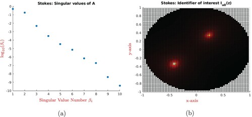
5.2.1. Two inhomogeneities

In the first numerical experiment, we take two homogeneous disks $B_1$ and $B_2$, respectively, centred at $z_1=(0.21,0.32)$ and $z_2=(-0.43,-0.35)$, to be retrieved using n = 10 source points. Let $u_0=e_1+e_2$, and $I_{u_0}\left(z\right):=I_{u_0}^{\left(1\right)}\left(z\right)$. Then the plots of $z\mapsto I_{u_0}\left(z\right)$ illustrate the results, where sharp peaks are expected to occur at the locations $z_j$ (j = 1, 2) of the inhomogeneities. We notice that there are two cases of interest: $\delta >T$ and $\delta \le T$.

For the case $\delta >T$ we choose $\delta =2.5$ and T = 1. The singular values are displayed in Figure 1(a) while the identifier of interest $I_{u_0}\left(z\right)$ is displayed in Figure 1(b). The image is obtained by using the first 4 largest singular vectors associated, of course, with the 4 largest singular values of the matrix A, respectively. The gaps in the representation of the singular values of A are not as distinct as in [4], however the two inhomogeneities are clearly discriminated from the background in 5.1(b). Their exact visual aspect depends on the choice of u0.

Figure 1. T = 1, $\delta =2.5$: (a) distribution of the singular values of A for n = 10 source points; (b) gloss level map of $I_{u_0}\left(z\right)$, $u_0=e_1+e_2$, for $z\in \mathrm{\Omega }$.

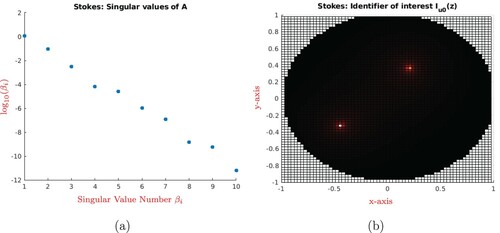
For the case $\delta \le T$ we choose $\delta =2.5$ and T = 3. In Figure 2(a), we see the distribution of the singular values of the matrix A. Figure 2(b) shows the identifier of interest $I_{u_0}\left(z\right)$, where the image is again obtained by using the first 4 largest singular vectors associated.

Figure 2. T = 3, $\delta =2.5$: (a) distribution of the singular values of A for n = 10 source points; (b) gloss level map of $I_{u_0}\left(z\right)$, $u_0=e_1+e_2$, for $z\in \mathrm{\Omega }$.

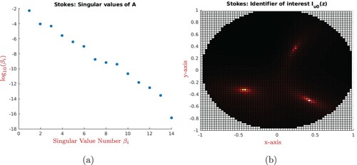
5.2.2. Three inhomogeneities

In the last numerical example, we add one more homogeneous disk $B_3$ with the same diameter $\alpha =0.1$, centred at $z_3=(0.4,-0.51)$ and having the viscosity ${\mu }_3=3$. For $\delta =4$, T = 1, the results are shown in Figure 3 where we get the distribution of the singular values of matrix A for 14 source points and the identifier of interest $I_{u_0}\left(z\right)$ for $u_0=e_1$. The image is obtained by using the first 6 largest singular vectors associated. The inhomogeneities are clearly discriminated from the background.

Figure 3. T = 1, $\delta =4$: (a) distribution of the singular values of A for n = 14 source points; (b) gloss level map of $I_{u_0}\left(z\right)$, $u_0=e_1$, for $z\in \mathrm{\Omega }$.

Disclosure statement

No potential conflict of interest was reported by the authors.

Additional information

Funding

This work is partially supported by Institute for Advanced Studies and AGM Research Center in Mathematics (UMR CNRS 8088), CY Cergy Paris University, F-95302 France.

References

- Afraites L, Dambrine M, Eppler K, et al. Detecting perfectly insulated obstacles by shape optimization techniques of order two. Discrete Contin Dyn Syst Ser B. 2007;8(2):389–416, (electronic).
- Alvarez C, Conca C, Friz L, et al. Identification of immersed obstacles via boundary measurements. Inverse Probl. 2005;21:1531–1552.
- Ammari H, Garapon P, Kang H, et al. Effective viscosity properties of dilute suspensions of arbitrarily shaped particles. Asymptot Anal. 2012;80:189–211.
- Badra M, Caubet F, Dambrine M. Detecting an obstacle immersed in a fluid by shape optimization methods. Math Models Methods Appl Sci. 2011;21(10):2069–2101.
- Ben Abda A, Hassine M, Jaoua M, et al. Topological sensitivity analysis for the location of small cavities in Stokes flow. SIAM J Control Optim. 2009;48(5):2871–2900.
- Bonnetier E, Manceau D, Triki F. Asymptotic of the velocity of a dilute suspension of droplets with interfacial tension. Q Appl Math. 2013;71:89–117.
- Caubet F, Dambrine M. Localization of small obstacles in Stokes flow. Inverse Probl. 2012;28:105007.
- Ammari H, Iakovleva E, Kang H, et al. Direct algorithms for thermal imaging of small inclusions. Multiscale Model Simul: SIAM Interdisciplinary J. 2005;4:1116–1136.
- Ammari H, Garapon P, Kang H, et al. A method of biological tissues elasticity reconstruction using magnetic resonance elastography measurements. Q Appl Math. 2008;66:139–175.
- Daveau C, Douady DM, Khelifi A, et al. Numerical solution of an inverse initial boundary-value problem for the full time-dependent Maxwell's equations in the presence of imperfections of small volume. Appl Anal. 2013;92(5):975–996.
- Daveau C, Khelifi A, Balloumi I. Asymptotic behaviors for eigenvalues and eigenfunctions associated to Stokes operator in the presence of small boundary perturbations. J Math Phys Anal Geom. 2017;20:13.
- Ikehata M. Reconstruction of inclusion from boundary measurements. J Inverse Ill-posed Probl. 2002;10(1):37–66.
- Jackson NE, Tucker CL. A model for large deformation of an ellipsoid droplet with interfacial tension. J Rheol. 2003;47:659–682.
- Maatoug H, Rakia M. Topological asymptotic formula for the 3D non-stationary Stokes problem and application. Revue Africaine de la Recherche en Informatique et Mathématiques Appliquées, INRIA, 2020, Volume 32 - 2019–2020. hal-01851477v2.
- Daveau C, Luong THC. Asymptotic formula for the solution of the Stokes problem with a small perturbation of the domain in two and three dimensions. Complex Var Elliptic Equ. 2014;59(9):1269–1282.
- Bonnetier E, Triki F. Asymptotics in the presence of inclusions of small volume for a conduction equation: A case with a non-smooth reference potential. AMS, Contemp Math Ser. 2009;494:95–112.
- Kwon O, Seo JK, Yoon JR. A real-time algorithm for the location search of discontinuous conductivities with one measurement. Commun Pure Appl Math. 2002;55:1–29.
- Beilina L, Klibanov MV. A globally convergent numerical method for a coefficient inverse problem. SIAM J Sci Comput. 2008;31(1):478–509.
- Beilina L, Klibanov MV, Kokurin MY. Adaptivity with relaxation for ill-posed problems and global convergence for a coefficient inverse problem. J Math Sci. 2010;167:279–325.
- Bellassoued M, Imanuvilov O, Yamamoto M. Carleman estimate for the Navier–Stokes equations and an application to a lateral Cauchy problem. Inverse Probl. 2016;32(2):025001, 23 pp.
- Choulli M, Imanuvilov OY, Puel J-P, et al. Inverse source problem for linearized Navier–Stokes equations with data in arbitrary sub-domain. Appl Anal. 2013;92(10):2127–2143.
- Boyer F, Fabrie P. Mathematical tools for the study of the incompressible Navier–Stokes equations and related models. New York (NY): Springer; 2013. (Applied mathematical sciences; vol. 183).
- Ladyzhenskaya OA. Mathematical theory of the viscous incompressible id. Moscow: Fizmathiz; 1961. p. 203
- Temam R. Navier–Stokes equations. Providence (RI): AMS Chelsea Publishing; 2001, Theory and numerical analysis, Reprint of the 1984 edition.
- Ammari H, Iakovleva E, Kang H. Reconstruction of a small inclusion in a two-dimensional open waveguide. SIAM J Appl Math. 2005;65(6):2107–2127.
- Cheney M. The linear sampling method and the MUSIC algorithm. Inverse Probl. 2001;17:591–595.
- Kirsch A. The MUSIC algorithm and the factorisation method in inverse scattering theory for inhomogeneous media. Inverse Probl. 2002;18:1025–1040.