A New Approach to Analytical Modeling of Mars’s Magnetic Field

ABSTRACT

A new three-staged technique based on various versions of the linear integral representation method (S-, F- and R-approximations) is applied to solve the problem of analytical modelling of the magnetic field on the surface of Mars. At the first step, we build an analytical approximation from the given data set (in local or regional cases). In the second step, we analyze the previous stage results and solve an ordinary differential equation system to find the integral curve of the gravity or magnetic field. The points of this curve are included in an extended data set, and we repeat the procedure described above for the first stage. The final approximation of the anomalous field elements or the topographic data allows us to find various linear transformations of the field under investigation, e.g. higher derivatives of the potential or Fourier-spectra of the field elements.

Analytical downward continuations of the magnetic field of Mars at various distances, including the planet's surface is presented.

KEYWORDS:

• S-approximation method
• analytic downward continuation
• magnetic field
• Mars
• regularization
• integral representation

Introduction

The study of a planet's magnetic field is one of the tools for improving our knowledge of its interior structure, evolution, and thermal history. Information on the magnetic fields of the planets became possible thanks to the planetary missions. A Martian era began in 1962 with the Soviet launch of Mars 1. Since then, Mars was visited by numerous spacecrafts. However, not all of them were successful or pass nearby the surface and have instruments to measure magnetic fields. The first result was obtained by US mission Mariner 4: no magnetosphere was observed on Mars, and if Mars had an intrinsic magnetic field, it turned out to have a minimal magnitude. In the 1970s, according to the Soviet Mars 2, 3, and 5 missions, and later Phobos 2, the intensity of magnetic field equal to about 60 nT at the equator and 120 nT at the pole spoke in favour of the absence of an intrinsic field [1].

Launched in 1996, the Mars Global Surveyor mission (MGS) with the magnetometer/electron reflectometer (MAG-ER) onboard has performed measurements at varying altitudes above the surface and provided the first unambiguous detection of the intrinsic magnetic field of Mars. See [2] for details of the mission's orbits and altitudes.

It was found that the Martian crust is intensely locally magnetized, and though Mars does not have a global magnetic field of internal origin at present, it could have had an active dynamo early in its history [3]. The MGS data allowed to map the global distribution of magnetic sources in the crust [4], and then using more effective tools to get a much-improved map of the field [5].

Many of the methods and tools developed to investigate the magnetic field on Earth can be applied to understand Martian crustal magnetism. A common technique is source modelling when the observed magnetic field is reached by locating some thin plates or prisms as magnetized sources somewhere beneath the surface. However, the solution is nonunique. Another well-known method is the continuation of a field: upward from the surface or downward. However, applying this procedure, one should keep in mind that downward continuation contains a differencing operation, and it can amplify short-wavelength noise.

There have been a lot of attempts to model local (the intensely magnetized southern highlands with strong magnetic anomalies reaching1500 nT at 200 km altitude) maps [6–8] and global maps of the magnetic field produced by remanent magnetism in the Martian crust, that can be divided into ‘spherical harmonic expansions’ models [9,10] and ‘equivalent source’ models [11,12].

The MGS magnetometer dataset is mainly obtained at 370-430 km orbit altitudes, while some data are available at 90-170 km orbits. Current crustal magnetic field models [13,14] consider the MAVEN magnetometer dataset at an altitude of about 135 km [2]. Thus, the altitude of orbital observations determines the spatial resolution of current models about 135 km. If the spatial scale of magnetic spots is significantly smaller than 135 km, the orbital measurements cannot detect them. It is essential to have magnetic field data at lower latitudes (from kilometres to tens of kilometres) to increase the models’ accuracy [15].

Nowadays is an exciting time for testing new methods and models of the magnetic field of Mars. The InSight lander operating on Mars has a magnetometer, which has provided the magnetic field measurements at the surface for the first time [16]. The available models failed to predict the amplitude of the magnetic field near the InSight landing site accurately. It turns out that the magnetic field intensity at the surface (>2000 nT) is ten times stronger than that predicted from the orbital sampling. The sources of magnetic field amplitudes are assumed to be buried by between 200 m to about 10 km of lava flows [16].

At the moment, InSight data are the only data obtained at the surface. On 14 May 2021, CNSA's (China National Space Administration) Tianwen-1 lander successfully landed on Mars. This gives us hope to have the magnetic field measurements at another point on the Martian surface.

The magnetic carries in the crust of Mars serve as an imprint of its evolutionary history. Martian dynamo models are based on these data [17]. The discrepancy between model values and the measured values at the surface motivates elaborating other methods that can help to obtain amplitudes and distribution of magnetic field sources on Mars. That is why we propose to apply a new technique to solve the problem of analytical modelling of the magnetic field on the surface of Mars.

Quite a long time ago (at least in the 19th-20th centuries), an idea arose to compare the field elements’ values at different points on the planet's surface with certain analytical expressions [18–22]. This idea could help solve various problems. The determination of appropriate analytical approximations usually requires regularization [23–26]. A well-known example represents the global magnetic and gravitational fields’ potentials using truncated series of spherical harmonics.

However, till quite recently, neither geophysicists nor geodesists used the idea of metrological analytical approximations of anomalous magnetic and gravity fields and also planet surface relief values in regional, local and global models systematically. This situation was due to two reasons:

1. the lack of a sufficiently general mathematical theory for constructing such metrological approximations;

2. insufficient availability of computing power.

Nevertheless, the situation has changed dramatically over the past decades. Namely, researchers have created practical tools for solving linear and nonlinear inverse problems in the integral representations method framework, including developed and tested applied programmes. For instance, in [27] the authors proposed the inflection point regularization method for solving one dimensional linear inverse problems. The optimal regularization method for high dimensional linear inverse problems (e.g. convolution equations) was investigated in [28]. A class of accelerated regularization methods for linear inverse problems was introduced in [29]. In [30], the authors developed several non-negativity preserving iterative regularization methods for general ill-posed inverse problems with non-negativity constraints. Thus, we can assert that the transition to a new approach in the theory of interpretation is over. This approach must include the following components:

1. original observed data;

2. analytical approximations of different field elements.

The paper organized is as follows. First, we describe the applied method, then describe the mathematical experiment and present our results.

In this work, we use only a priori known information about the magnetic field: the intensity magnetic field model [14] obtained from a set of satellite measurements at different altitudes and the value of magnetic anomaly at the InSight landing site.

Method

We briefly mention the essence of the linear integral representations method [31–35].

Let $N$ values be given ($N$ is large enough, conditionally: $N\ge {10}^4$) (1) $f_{i,\delta }=f_i+\delta f_i,i=\overline{1,N},$(1) where $f_i$ are useful signals, and $\delta f_i$ – noise, and the relations hold (2) $f_i=\sum _{r=1}^R\underset{M_r}{\int }{\rho }_r(\xi )Q_r^{(i)}(\xi )d{\mu }_r(\xi ),$(2) where $M_r$ are connected point sets (in general case in ${\mathbb{R}}^n,i\ge 1$), ${\mu }_r(\xi )$ – given measures on $M_r$, $Q_r^{(i)}(\xi ),r=\overline{1,R},i=\overline{1,N},$ are given functions, for example, the first derivatives of the gravitational or magnetic potential at the point $\xi$. $M_r$ represents the support of the magnetic or gravity masses. It can be one-, two- or three-dimensional. In our case such support is a sphere with a radius greater than the mean Mars’s radius. The dimension of ${\mathbb{R}}^n$ can be two or three. It is the space around the planet under consideration. ${\rho }_r(\xi )$ are functions to be found. ${\rho }_r(\xi )$ can be the density of a simple or double layer distributed on a plane or a sphere. We can consider this density as a projection of real sources to the support of magnetic masses. Real masses are of cause three-dimensional. The method of finding ${\rho }_r(\xi )$ (finding the integral representations of values $f_i,i=\overline{1,N}$) consists in setting and solving the following conditionally extreme problem (3) $\begin{array}{l}F(\rho )=\sum _{r=1}^R\underset{M_r}{\int }{\displaystyle \frac{{\rho }_r^2(\xi )}{p_r^2(\xi )}}d{\mu }_r(\xi )=\underset{{\rho }_r(\xi )}{\text{min}},\\ f_{i,\delta }-\sum _{r=1}^R\underset{M_r}{\int }{\rho }_r(\xi )Q_r^{(i)}(\xi )d{\mu }_r(\xi )=0,i=\overline{1,N}.\end{array}$(3) Here $p_r^2(\xi )$ are given functions. $p_r^2(\xi )$ reflects the boundary conditions. We may set the function values to zero if the observation point belongs to the boundary of the support. This function can play the significant role if we are to deal with several regions with topographies which differ one from another dramatically. This case takes place on Mars. We can find an analytical approximation for each domain and then compare the results in the intersection. $p_r^2(\xi )$ can characterize the features of the intersection area and should be considered as a weight-function in this case.

The problem (3) is reduced to a set of unconditional variational problems by means of Lagrange factor method (4) $F(\rho )+2\sum _{r=1}^R{\lambda }_i\left(f_{i,\delta }-\sum _{r=1}^R\underset{M_r}{\int }{\rho }_r(\xi )Q_r^{(i)}(\xi )d{\mu }_r(\xi )\right)=\underset{{\rho }_r(\xi )}{\text{min}}.$(4) In addition, (4) are the Lagrange factors which are components of the Lagrange vector $\lambda$. The solutions ${\tilde{\rho }}_r(\xi ;\lambda )={\rho }_r(\xi ),r=\overline{1,R},$ of problem (4) have the form: (5) ${\tilde{\rho }}_r(\xi ;\lambda )=p_r^2(\xi )(\lambda ,Q_r(\xi )),$(5) where $Q_r(\xi )$ is the $N$-vector with components $Q_r^{(i)}(\xi ),i=\overline{1,N}$. Vector $\lambda$ is found from the solution of linear algebraic equation system (6) $A\lambda =f_{\delta }=f+\delta f,$(6) where $f_{\delta }$ – $N$-vector with components $f_{i,\delta }$, $f$ and $\delta f$ are $N$-vectors of useful signal and noise respectively with components $f_i$ and $\delta f_i,i=\overline{1,N}$.

The primary method of finding functions ${\rho }_r(\xi )$ is an iterative one, like the gradient decent approaches or their continuous analogs such as asymptotical regularization methods, see e.g. [36,37]. At each step of the iteration process, a correction compared with the preceding step is made using the linear integral representation method.

Let us explain the idea of constructing metrological linear analytical approximations of anomalous magnetic or gravity field elements. The essence of these approximations lies in the following. If $f_{i,\delta }$ are given observed values of one (or even several at once – in the same points or different points on the planet's surface and (or) in outer space) external anomalous magnetic field, then they are represented in the form (1)-(2), the sets $M_r$ being given without the use of any information about sources of the anomalous field of a quantitative kind. That's why these approximations are called metrological.

For the same observed field data, there can be found various metrological linear integral approximations. This fact is in some sense of crucial importance.

The central computing procedure in the linear integral representation method is finding a stable approximate solution of SLAE (6), the approximate representation (but accurate enough as a rule) of noise $\delta f$ also being found. In the case of the external anomalous field, this means that the component of the external field is found, which is caused by the heterogeneities in the upper (surface, of power up to 50–100 m in the vertical dimension) layer of the planet; this moment is a matter of principle.

We will use the integral representation (3) to find the spatial distribution of the elements and localize the sources of a potential field. Specifically, we record the main formula of harmonic function theory for the halfspace bounded by the plane $x_3=0$ (from now on referred to as the $\mathrm{\Pi }$–plane) [1]: (7) $\begin{array}{rl}V(M)& =\underset{-\mathrm{\infty }}{\overset{+\mathrm{\infty }}{\int }}\underset{-\mathrm{\infty }}{\overset{+\mathrm{\infty }}{\int }}{\displaystyle \frac{{\rho }_1({\xi }_1,{\xi }_2)d{\xi }_{1}d{\xi }_2}{\sqrt{{(x_1-{\xi }_1)}^2+{(x_2-{\xi }_2)}^2+x_3^2}}}\\ & +\underset{-\mathrm{\infty }}{\overset{+\mathrm{\infty }}{\int }}\underset{-\mathrm{\infty }}{\overset{+\mathrm{\infty }}{\int }}{\displaystyle \frac{{\rho }_2({\xi }_1,{\xi }_2)x_{3}d{\xi }_{1}d{\xi }_2}{{\left(\sqrt{{(x_1-{\xi }_1)}^2+{(x_2-{\xi }_2)}^2+x_3^2}\right)}^3}},\\ M& =(x_1,x_2,x_3),\xi =({\xi }_1,{\xi }_2,{\xi }_3).\end{array}$(7) We selected the coordinate system so that the plane of the simple and double layer be specified by equation $x_3=0$. Then, the derivative of potential $V$ with respect to $x_3$ taken with the opposite sign has the following form: (8) $\begin{array}{rl}-\frac{\mathrm{\partial }V(M)}{\mathrm{\partial }{x}_3}& =\underset{-\mathrm{\infty }}{\overset{+\mathrm{\infty }}{\int }}\underset{-\mathrm{\infty }}{\overset{+\mathrm{\infty }}{\int }}\frac{{\rho }_1(\hat{\xi })x_{3}d\hat{\xi }}{{\left(\sqrt{{(x_1-{\xi }_1)}^2+{(x_2-{\xi }_2)}^2+x_3^2}\right)}^3}\\ & +\underset{-\mathrm{\infty }}{\overset{+\mathrm{\infty }}{\int }}\underset{-\mathrm{\infty }}{\overset{+\mathrm{\infty }}{\int }}\frac{{\rho }_2(\hat{\xi })(2x_3^2-{(x_1-{\xi }_1)}^2-{(x_2-{\xi }_2)}^2)d\hat{\xi }}{{\left(\sqrt{{(x_1-{\xi }_1)}^2+{(x_2-{\xi }_2)}^2+x_3^2}\right)}^5},\\ M& =(x_1,x_2,x_3),\hat{\xi }=({\xi }_1,{\xi }_2).\end{array}$(8) Functions ${\rho }_1,$ ${\rho }_2$ are not known. Let the components of the field be specified in a finite set of points $M_i=(x_1^{(i)},x_2^{(i)},x_3^{(i)}),i=\overline{1,N}.$We denote the integration function in the first term of (8) at point $M_i$ by $Q_1^{(i)}$ and in the second term by $Q_2^{(i)}$. Hence, we obtain: (9) $-\frac{\mathrm{\partial }V(M)}{\mathrm{\partial }{x}_3}=\underset{-\mathrm{\infty }}{\overset{+\mathrm{\infty }}{\int }}\underset{-\mathrm{\infty }}{\overset{+\mathrm{\infty }}{\int }}({\rho }_1(\hat{\xi })Q_1^{(i)}(\hat{\xi })+{\rho }_2(\hat{\xi })Q_2^{(i)}(\hat{\xi }))d\hat{\xi },i=\overline{1,N}.$(9) It should be noted that formulas (8)-(9) are the backbone for constructing S–approximations of the sought element of the anomalous potential field in the so-called local case (when the sphericity of the planet is not taken into account).

We should reflect a significant fact: integral representations of the anomalous potential fields (i.e. the fields that are harmonic in some domains of the space of sourcewise functions) are closely linked. The formulas for matrix elements in the method of local S–approximations are [1]: (10) $\begin{array}{l}{a}_{ij}=2\pi \left\{{\displaystyle \frac{z_i+z_j}{{\rho }_{ij}^3}}+{\displaystyle \frac{(z_i+z_j)(9{\rho }_{ij}^2-6{(z_i+z_j)}^2)}{{\rho }_{ij}^7}}\right\},\\ {\rho }_{ij}^2=(z_i+z_j{)}^2+(x_i-x_j{)}^2+(y_i-y_j{)}^2,1\le i,j\le N.\end{array}$(10) The question of what method is to be used by constructing linear metrological approximation of anomalous field elements for tremendous territories with the number of observed data $N=n\cdot {10}^6,1<n<10$ is a matter of principle. (For example, one should build linear approximations for the field $\mathrm{\Delta }g(x)=-\frac{\mathrm{\partial }{V}_a(x)}{\mathrm{\partial }r}$ on a scale of 1:200 000 for the area of whole Russia or whole Europe). The solution to this problem is reached due to the implementation of the composite local approximation method. Exactly, let the area of Russia (respectively – of Europe) be a set of sheets on a scale of 1:200 000. We will build its approximation of the field $\mathrm{\Delta }g(x)=-\frac{\mathrm{\partial }{V}_a(x)}{\mathrm{\partial }r}$ for each sheet, using observed data on this sheet and eight other adjacent ones and 16 sheets adjacent to the adjacent ones. The number of data from which an approximation will be made will be about $n\cdot {10}^4,n\le 5$, and the corresponding SLAE will be solved effectively.

Also, one should use a series of tricks (to be considered in the paper), ensuring a high degree of coordination for linear metrological integral approximations made over adjacent sheets.

A pretty similar technique is used in finding metrological linear approximations of the Earth’s relief. The case of a magnetic field is rather complicated because we must use the nonlinear integral representation method in case of strong anomalies $\mathrm{\Delta }{T}_a$.

Now, we are to point out how our approach is implemented in the regional case when a planet's form plays a significant role.

Let an idealized model of the planet be the interior of a sphere having radius $R$. The real planet is treated as a domain bounded by a closed piecewise-continuous surface $S$ insignificantly deviating from the sphere of the radius $R_0$ located within the interior of this domain (we do not consider the ellipticity of the planet's shape in this paper). It is assumed that approximate values of a function $V(x)$, harmonic outside the sphere, are specified on an arbitrary set of points $x^{(i)},i=\overline{1,N}$ on the surface $S$: (11) $\begin{array}{l}{f}_{i,\delta }=f_i+\delta f_i,\\ f_i=V(x^{(i)}),\\ i=\overline{1,N}.\end{array}$(11) Since $V(x)$ is harmonic at $r>R_0$, it has the following integral representation: (12) $\begin{array}{rl}V(x)& =\frac{R_0^2}{4\pi }\underset{0}{\overset{2\pi }{\int }}\underset{0}{\overset{\pi }{\int }}\frac{\sigma (\vartheta ,\phi )\sin \vartheta d\vartheta d\phi }{R_{\xi -x}}\\ & +\frac{R_0^2}{4\pi }\underset{0}{\overset{2\pi }{\int }}\underset{0}{\overset{\pi }{\int }}\frac{w(\vartheta ,\phi )(R_0-r\cos {\vartheta }^{\mathrm{\prime }})\sin \vartheta d\vartheta d\phi }{R_{\xi -x}^3},\\ R_{\xi -x}& =\sqrt{R_0^2-2R_{0}r\cos {\vartheta }^{\mathrm{\prime }}+r^2},\\ \xi & =R_0(\cos \phi \sin \vartheta ,\sin \phi \sin \vartheta ,\cos \vartheta ),\\ x& =r(\cos \tilde{\phi }\sin \tilde{\vartheta },\sin \tilde{\phi }\sin \tilde{\vartheta },\cos \tilde{\vartheta }),\\ & \cos {\vartheta }^{\mathrm{\prime }}=\sin \vartheta \sin \tilde{\vartheta }\cos (\phi -\tilde{\phi })+\cos \vartheta \cos \tilde{\vartheta }.\end{array}$(12) The function $\sigma (\vartheta ,\phi )$ in (12) is called the density of a simple layer distributed over the sphere of radius $R_0$, the function $w(\vartheta ,\phi )$ is the density of a double layer (distributed over the same sphere), and $R_{\xi -x}$ is the distance between the current point $\xi$ on the sphere and the observation point $x$. Differentiating the right-hand side in (12) with respect to various coordinates, integral representations of the respective derivatives of $V(x)$ can be obtained, even if these derivatives (e.g. $\mathrm{\partial }V/\mathrm{\partial }r$) are nonharmonic functions.

Formula (12) is a different form of the integral representation of a function harmonic outside a sphere of radius R [38]: (13) $V(x)=\frac{1}{4\pi }\underset{0}{\overset{2\pi }{\int }}\underset{0}{\overset{\pi }{\int }}\left(\frac{1}{R_{\xi -x}}\frac{\mathrm{\partial }V(\xi )}{\mathrm{\partial }\overrightarrow{n}}-V(\xi )\frac{\mathrm{\partial }}{\mathrm{\partial }\overrightarrow{n}}\left(\frac{1}{R_{\xi -x}}\right)\right)\sin \vartheta d\vartheta d\phi ,$(13) where $\overrightarrow{n}$ is outer normal to the unit sphere (we can write $\mathrm{\partial }/\mathrm{\partial }r$, where $r$ is the radial coordinate of the radius-vector $\overrightarrow{x}$).

A conditional variation problem for $\sigma$ and $w$ [32] has the solution (14) $\begin{array}{rl}\sigma (\hat{\xi })& =\sum _{i=1}^N{\lambda }_i{Q}_i^{(1)}(\xi ),w(\hat{\xi })=\sum _{i=1}^N{\lambda }_i{Q}_i^{(2)}(\xi ),\hat{\xi }=(\vartheta ,\phi ),\\ Q_i^{(1)}(\xi )& =\frac{1}{R_{\xi -x^{(i)}}},Q_i^{(2)}(\xi )=\frac{R_0-r_i\cos {\vartheta }_I^{\mathrm{\prime }}}{R_{\xi -x^{(i)}}^3}.\end{array}$(14) The quantities ${\lambda }_i$ are the components of an N-vector $\lambda$ providing the solution to the system of linear equations like (6) described above and the vector $f_{\delta }$ consists of components $f_{i,\delta }$ (see (11)), and the elements of the matrix $A=A^T\ge 0$ are (15) $\begin{array}{rl}{a}_{ij}& =a_{ji}=\underset{0}{\overset{2\pi }{\int }}\underset{0}{\overset{\pi }{\int }}(Q_i^{(1)}(\xi )Q_j^{(1)}(\xi )+Q_i^{(2)}(\xi )Q_j^{(2)}(\xi ))\sin \vartheta d\vartheta d\phi \\ & =\frac{2\pi }{r_i{r}_j\sqrt{h_i{h}_j}}\left(1+\frac{1}{4r_i{r}_j{h}_i{h}_j}\right)\times \text{F}\left(2\text{arctg}\left(\sqrt{h_i{h}_j}\right),\sqrt{\frac{1+\cos ({\alpha }_{ij})}{2}}\right)-\\ & -\frac{\pi (3h_i^2{h}_j^2-4h_i{h}_j\cos ({\alpha }_{ij})+1)}{r_i^2{r}_j^2{h}_i{h}_j{\left(\sqrt{1-2h_i{h}_j\cos ({\alpha }_{ij})+h_i^2{h}_j^2}\right)}^3}.\end{array}$(15) Here $h_i=R_0/r_i,i=\overline{1,N},h_j=R_0/r_j,j=\overline{1,N},{\alpha }_{ij}$is the angle between the vectors $x_i$ and $x_j$. We can suppose that the vector $x_i$ is parallel to the axis $Oz$ and the vector $x_j$ lies in the plane $xOz$ (we can choose such a coordinate system). Then these vectors have the coordinates $x_i=r_i(0,0,1)$ and $x_j=r_j(\sin {\alpha }_{ij},0,\cos {\alpha }_{ij})$. The function $F(\phi ,k)$ is an elliptic integral of the second order [39,40].

Contrary to the technique described in other papers [34,41], we suggest a mathematical formalization of the properties for the solution to the inverse problem. Functions ${\tilde{p}}_r^{(k)},r=\overline{1,R},k=1,2,\dots$ are not constants and the representations hold (16) ${\tilde{p}}_r^{(k)}(\xi )=\sum _{i=1}^N{\gamma }_i^{(r)}{Q}_r^{(i)}(\xi ),r=\overline{1,R}.$(16) Expressions (16) reflect the dependencies of functions ${\tilde{p}}_r^{(k)},r=\overline{1,R},k=1,2,\dots$ on the given field element and simple- and double-layer carriers. To avoid numerical computing of the matrix elements (which causes random errors in the solution to SLAE), we set some additional constraints for these functions to obey. Namely, we require that the functions ${\tilde{p}}_r^{(k)}(\xi )$ are harmonic outside the mass carrier. In this case, the matrix elements can be calculated from the following formula (17) $a^{{\circ }_{ij}}{}^{(r)}=\sum _{l=1}^N{\gamma }_l^{(r)}\underset{M_r}{\int }{\tilde{Q}}_r^{(l)}(\xi )Q_r^{(i)}(\xi )Q_r^{(j)}(\xi )d{\mu }_r(\xi ),r=\overline{1,R},i=\overline{1,N},j=\overline{1,N}.$(17) If the sources of magnetic masses are distributed on the horizontal plane lying at a depth of H beneath Mars’s surface, then these elements have the form (18) $\begin{array}{rl}{a}_{ij}^{\circ }{}^{(r)}& =\sum _{l=1}^N{\gamma }_l^{(1)}\frac{x_i-x_j}{{\left(\sqrt{{(x_i-x_j)}^2+{(y_i-y_j)}^2+{(z_i+z_j+2H)}^2}\right)}^3}\\ & \times \frac{x_i-x_l}{{\left(\sqrt{{(x_l-x_i)}^2+{(y_l-y_i)}^2+{(z_i+z_l+2H)}^2}\right)}^3}\\ & +\sum _{l=1}^N{\gamma }_l^{(2)}(\frac{\mathrm{\partial }}{\mathrm{\partial }{z}_i}(\frac{2({(x_i-x_j)}^2+{(y_i-y_j)}^2)-{(z_i+z_j+2H)}^2}{{\left(\sqrt{{(x_i-x_j)}^2+{(y_i-y_j)}^2+{(z_i+z_j+2H)}^2}\right)}^5}\\ & \times \frac{2({(x_l-x_i)}^2+{(y_l-y_j)}^2)-{(z_i+z_l+2H)}^2}{{\left(\sqrt{{(x_l-x_i)}^2+{(y_l-y_i)}^2+{(z_i+z_j+2H)}^2}\right)}^5})),\\ i& =\overline{1,N},j=\overline{1,N}.\end{array}$(18) In this case, we have only two carriers: those are two copies of the same horizontal plane.

The coefficients ${\gamma }_l^{(r)},l=\overline{1,N},r=\overline{1,R}$ should satisfy the following homogeneous system of linear algebraic equations (SLAE, as noticed above): (19) $\sum _{l=1}^N{\gamma }_l^{(r)}(\mathrm{\nabla }{\tilde{Q}}_r^{(l)}(x_i),\mathrm{\nabla }{Q}_r^{(j)}(x_i))=0,r=\overline{1,R},i=\overline{1,N}$(19) The equation (19) is the orthogonality condition of two vectors on the carrier $M_r,r=\overline{1,R}$.

System (19) is regularized and then solved; some additional constraints are imposed on the coefficients to be found. These constraints depend on the setting. The simplest way to choose a valid solution to (19) is to limit the varying range of some quantitative characteristics of the simple and double layer's densities (see (14)-(15)).

Our new approach for finding stable linear transformation of a planet's physical fields can be explained as follows.

1. At the first stage, we create an analytical S-approximation of the field element. It also can be the S-, F- or R-approximation [34,42,43,44] or a combined one. The solution to SLAE, which fully describes the inverse problem in this situation, gives the coefficients’ values in expressions (17). Thus, we can find the field values in a neighbourhood of the given data set, especially when a space vehicle's trajectory is considered. Designing Mars's magnetic field's analytical approximations implies the combined implementation of local (7) and regional (12) versions of the S-approximation method. Firstly, we build a regional approximation (12) of a data set to perform a series of continuous descents of this field towards the surface. Then we create a local S-approximation (7) for refining our construction and revealing some new features of the equivalent sources. The distribution of such sources is mapped, and we can evaluate the characteristics of them.

2. The computed at the previous stage field values are the start point of an integral curve corresponding to the investigation vector field. So, the second stage of our method is, in fact, the solution of a system of ordinary differential equations regulated by the Hamiltonian of form (20) $\mathcal{H}(\overrightarrow{x},\overrightarrow{y},\overrightarrow{z})=\sum _{i=1}^N\{V_{xi}^2+V_{yi}^2+V_{zi}^2\}.$(20)

Here $\overrightarrow{x}=(x_1,x_2,\dots ,x_N)$, $\overrightarrow{y}=(y_1,y_2,\dots ,y_N)$, $\overrightarrow{z}=(z_1,z_2,\dots ,z_N)$ are the Cartesian coordinates of the observation data at the $i$-th point, $V_{xi},V_{yi},V_{zi}$ are the derivative’s values of the potential over the relating coordinate. The equation system for the integral curve looks like (21) $\begin{array}{rl}{\displaystyle \frac{dx}{dt}}& =X(x,y,z),{\displaystyle \frac{dy}{dt}}=Y(x,y,z),{\displaystyle \frac{dz}{dt}}=Z(x,y,z),\\ X(x,y,z)& =\sum _{i=1}^N{P}_i^{(1)}{\displaystyle \frac{x-x_i}{{\left(\sqrt{{(x-x_i)}^2+{(y-y_i)}^2+{(z-z_i+2H)}^2}\right)}^3}},\\ Y(x,y,z)& =\sum _{i=1}^N{P}_i^{(1)}{\displaystyle \frac{y-y_i}{{\left(\sqrt{{(x-x_i)}^2+{(y-y_i)}^2+{(z-z_i+2H)}^2}\right)}^3}},\\ Z(x,y,z)& =\sum _{i=1}^N{P}_i^{(1)}{\displaystyle \frac{z-z_i+2H}{{\left(\sqrt{{(x-x_i)}^2+{(y-y_i)}^2+{(z-z_i+2H)}^2}\right)}^3}}.\end{array}$(21) We should emphasize that even when the sphericity of a planet is taken into account, it is preferable (without loss of generality) to find the integral curves in cartesian coordinates because of our approach's local character.

The integral curve found at the second stage gives an additional data set for the further analytical approximations and continuous transformation of the magnetic field downwards toward Mars's surface. So, we gain stability in the continuation process.

The structural-parametric approach within the linear integral representation method is a generalization of the variational one. Namely, we should find vectors ${\lambda }^r,r=\overline{1,R}$ for every source of masses individually.

So, owing to (6) the problem of finding linear integral representations of values $f_i$ which is indefinite is reduced to the definite one – to the problem of finding a stable approximate solution of linear algebraic equation system (SLAE) (6) (because of the presence of noise it is not significant to find the precise solution). In the case of the structure-parametric approach, we have (22) $\stackrel{\circ }{A}\stackrel{\circ }{\lambda }=f_{\delta },$(22) where (23) $\stackrel{\circ }{\lambda }=\Vert \begin{array}{c}\stackrel{\circ }{\lambda }(1)\\ \stackrel{\circ }{\lambda }(2)\\ \dots \\ \stackrel{\circ }{\lambda }(R)\end{array}\Vert ,{\lambda }^{\circ }{}^{(r)}=\Vert \begin{array}{c}{\stackrel{\circ }{\lambda }}_1(r)\\ {\stackrel{\circ }{\lambda }}_2(r)\\ \dots \\ \stackrel{\circ }{\lambda }{}_N(r)\end{array}\Vert ,$(23) and the matrix $A^{\circ }$ has the following form (24) $\stackrel{\circ }{A}=\Vert \stackrel{\circ }{A}{}^{(1)}\stackrel{\circ }{A}{}^{(2)}\dots \stackrel{\circ }{A}{}^{(R)}\Vert .$(24) Here the blocks $\stackrel{\circ }{A}{}^{(r)}$ are filled with the elements (25) $\stackrel{\circ }{a}{}_{ij}^{(r)}=\underset{M_r}{\int }{\rho }_r(\xi )Q_r^{(i)}(\xi )Q_r^{(j)}(\xi )d{\mu }_r(\xi ),r=\overline{1,R},$(25) and are in general case not symmetric, that is the property (26) $\stackrel{\circ }{A}{}^{(r)}=\stackrel{\circ }{A}{}^{(r)},T\ge 0,r=\overline{1,R},$(26) can be violated.

It should be noted that such matrix, cf. (26), is called positive on a cone. For efficiently solving this type of linear inverse problems, one can use the adaptive sparse regularization algorithm or the Lagrange principle based methods, proposed in [45] and [46], respectively.

System (22) is very underdefined (it has N equations and NR unknown variables). We have elaborated the so-called block contrasting method with continuous block dimension deformation [47]. This method seems to be effective while solving such systems. It was tested on some series of geophysical and geodetic data sets. In the next section we will describe the results of the interpretation processes with the technique's help.

As we stressed above, a new three-staged technique based on various versions of the linear integral representation method (S-, F- and R-approximations) [34] is designed. The process of solving the inverse problems of geophysics and geodesy reduces to the following:

At the first step, we build an analytical approximation from the given data set (in local or regional case) solving system (6) or (22), matrix elements having the form (10), (15), or (25);

At the second step, we analyze the previous stage results and solve an ordinary differential equation system to find the integral curve of the gravity or magnetic field. The points of this curve are included in an extended data set, and we repeat the procedure described above for the first stage;

The final approximation of the anomalous field elements allows us to find various linear transformations of the field under investigation, e.g. higher derivatives of the potential or Fourier-spectra of the field elements.

In the next section we will demonstrate how our new method works. We should stress that the solution to SLAE is obtained with high accuracy, and we can cancel the lack of data at profile surveys by an analytical continuation along the integral curve of the magnetic field. The vector field components are calculated according to (5) and depend on the solution vector and the initial variational setting.

We note that in spherical coordinates, it is more appropriate to write the integral representation for the harmonic function $r\frac{\mathrm{\partial }V}{\mathrm{\partial }r}(r,\vartheta ,\phi )$ using formula (12) rather than to differentiate the corresponding expression for $V(r)$ because, in the latter case, the formulas for elements of the matrix A are more complicated and require higher accuracy of calculations (due to higher degrees of distances between the respective points).

Mathematical experiment on the analytical continuation of Mars’s magnetic field measured at the orbit of a spacecraft

We have considered several model examples. In all cases, we approximated the anomalous field by the sum of simple and double layers distributed over two spheres. Initially, the spheres’ depths of occurrence varied from 100 m to 50 km below the region's minimum relief. When solving system (6) using the improved method of block contrasting within the framework of the structural-parametric approach, the accuracy of approximation the magnetic field of Mars at an altitude of 200 km was $\mathrm{\Delta }=\frac{{||Ax-f_{\delta }||}_E}{{||f_{\delta }||}_E}={10}^{-6}$, where $||Ax-f_{\delta }|{|}_E$ and$||f_{\delta }|{|}_E$ are Euclidean norms of vectors $Ax-f_{\delta }$ and $f_{\delta }$ respectively.

Then we examined the region 20° S – 20° N, 120° E – 180° E over the southwestern part of the Elysium Planitia, in the InSight landing area (4.5024° N, 135.6234° E). We took the initial values from the global model of the magnetic field of Mars [14], obtained by the equivalent sources dipole method (ESD) from sample data of satellite measurements at different altitudes and presented at an altitude of 150 km in the form of spherical harmonics of 134 degree and order, which corresponds to the spatial resolution on the surface ∼ 160 km. The number of magnetic field induction vectors components over the area under consideration is 5043, which corresponds to 1681 selected points and a spatial resolution of 1°. We took a sphere with a radius of 3393.5 km as a reference surface.

We approximated the anomalous magnetic field by the sum of simple and a double layer distributed over two symmetric spheres. The depths of the spheres under the surface of the idealized planet in various experiments varied from 0.1 km to 50 km since the depths of the sources equivalent by the external magnetic field are the method's parameters. Varying these parameters during the analytic continuation of the field towards the sources did not significantly change the result; therefore, we selected the depths following a priori information on possible natural sources of remanent Mars magnetization. There is currently little such information, so we use common assumptions about the localization of magnetization sources in the planet's crust. We have paid more attention to suggested in [16] constraints to the depth of magnetization. We also performed various experiments with depths of magnetization varied from 0.1 km to 50 km as it's supposed now that Mars likely has a 24- to 72-kilometer-thick crust [48]. In all cases, the ratio of the Euclidean norm of the difference between the left and right sides to the Euclidean norm of the right side did not exceed 10⁻⁹ with different occurrence depths of equivalent magnetic mass carriers, which indicates sufficiently high accuracy of the approximation. Figure 1 shows quite an accurate approximation of the initial model data at an altitude of 150 km, as evidenced by the heat map and the frequency histogram of value differences.

Figure 1. Isoline maps of the total magnetic field B at an altitude of 150 km according to the source model data [14] obtained by (a) transformation using spherical harmonics and (b) solution of the inverse problem using modified S-approximations; (c) heat map of value differences between source model data and the result of S-approximations; (d) frequency histogram of value differences between (a) and (b).

Also, in all experiments, the field continuation retained its structure and relationship with the initial values at a distance of up to 60 km and more from the initial values, but at a distance of 90 km and further, the field ‘decayed,’ magnetic field components strongly increased in absolute value and often changed their sign. For this reason, the analytic continuation of the initial field to the planet's surface, taking into account the complex topography and comparison of the results with the data of the InSight magnetometer, seems to be insufficiently substantiated so far. Nevertheless, according to the analytic continuation, the predicted total magnetic field $B$ at the InSight landing site was 2680 nT, while the average value of $B$ measured by the InSight magnetometer is 2013 ± 53 nT [16].

The mass carriers selected for demonstration in this work, equivalent in the external magnetic field, are distributed over two concentric spheres lying at depths of 1 and 10 km below the reference surface, which corresponds to the assumed boundaries of magnetic masses in the Martian crust of ≈1-10 km [16].

We obtained the magnetic field components $B_{\theta }$, $B_{\phi }$, $B_r$ at an altitude of 150 km due to solving the inverse problem using modified S-approximations. Analytic continuations of the magnetic field over the area under consideration are plotted downward at distances of 30 km, 60 km, 90 km, and to the planet's surface, considering the relief.

Figures 2–5 compare the total magnetic field B at different altitudes according to the source model data [14] obtained by the transformation using spherical harmonics and our method of analytic downward continuations within modified S-approximations. As we move away from the initial data altitudes, the obtained results are getting inconsistent with source model transformations [14]. The discrepancies are due not only to the solution of the inverse problem that is not guaranteed to be unique or stable but also to the peculiarities of our method, particularly our model of the distribution of magnetic mass sources on two concentric spheres. At altitudes of 120-90 km, the pattern of the analytic downward continuation of the magnetic field within modified S–approximations is similar to the results of source model transformations using spherical harmonics [14]. Then further, as we approach the sources of magnetic masses, due to the features mentioned above and the chosen parameters of the method, we obtain a solution that significantly differs from the source model [14]. Near the planet's surface, the field is finally disintegrating that testifies to the proximity to the supposed sources of magnetic masses. Also, we have determined the quantitative (as mentioned in the Introduction, this paper deal only with metrological approximations of physical fields) behaviour of the simple layer densities at different depths. Figure 6 demonstrates the distribution of one sphere's magnetic sources, equivalent to the external magnetic field from the source model [14] at an altitude of 150 km.

Figure 2. Isoline maps of the total magnetic field B at an altitude of 120 km according to the source model data [14] obtained by (a) transformation using spherical harmonics and (b) analytic downward continuations within modified S-approximations; (c) heat map of value differences between (a) and (b); (d) frequency histogram of value differences between (a) and (b).

Figure 3. Isoline maps of the total magnetic field B at an altitude of 90 km according to the source model data [14] obtained by (a) transformation using spherical harmonics and (b) analytic downward continuations within modified S-approximations; (c) heat map of value differences between (a) and (b); (d) frequency histogram of value differences between (a) and (b).

Figure 4. Isoline maps of the total magnetic field B at an altitude of 60 km according to the source model data [14] obtained by (a) transformation using spherical harmonics and (b) analytic downward continuations within modified S-approximations; (c) heat map of value differences between (a) and (b); (d) frequency histogram of value differences between (a) and (b).

Figure 5. Isoline maps of the total magnetic field B on the surface according to the source model data [14] obtained by (a) transformation using spherical harmonics and (b) analytic downward continuations within modified S-approximations; (c) heat map of value differences between (a) and (b); (d) frequency histogram of value differences between (a) and (b).

Figure 6. Quantitative maps of the distribution of equivalent sources, using modified S-approximations at depths of (a) 1 km, (b) 10 km below the relief.

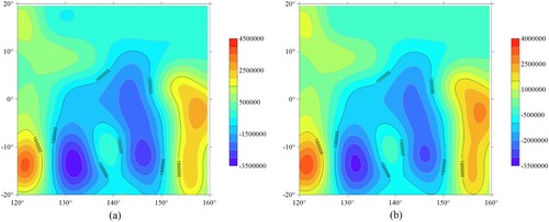
Table 1 shows some descriptive statistics for data obtained by transformations of the total magnetic field B according to the model [14] using spherical harmonics, our downward continuations within modified analytic S-approximations, and differences between them. The depths of two concentric spheres with magnetic sources under the surface of an idealized planet are 1 and 10 km.

Table 1. Descriptive statistics for data on the total magnetic field at different altitudes according to the spherical harmonics model (L), the model of S-approximations (S), and the difference between them (D).

Altitude-model	Minimum	Maximum	Mean	Median	Root Mean Square	Variance	Standard Deviation	Range
150-L	0,69	256,09	57,35	44,30	78,60	2890,09	53,76	255,40
120-L	1,00	361,08	78,98	58,56	108,95	5631,46	75,04	360,08
90-L	1,85	532,78	113,13	79,40	157,20	11914,14	109,15	530,93
60-L	1,04	860,20	170,46	112,71	239,63	28382,43	168,47	859,16
0-L	2,87	2762,79	454,89	295,65	640,75	203755,76	451,39	2759,93
150-S	0,57	257,23	57,74	44,31	79,35	2963,84	54,44	256,66
120-S	0,82	288,90	60,93	44,64	82,91	3164,05	56,25	288,08
90-S	1,23	377,91	76,15	56,99	69,98	4170,31	64,58	376,68
60-S	4,75	701,46	155,61	122,63	202,31	16726,91	129,33	696,71
0-S	17,56	15163,46	3950,82	2386,19	5373,73	13275910,34	3643,61	15145,90
150-D	−1,14E-06	1,48E-06	2,14E-07	1,93E-07	3,87E-07	1,04E-13	3,23E-07	2,62E-06
120-D	−35,09	111,85	18,04	10,69	29,16	525,04	22,91	146,94
90-D	−126,81	305,02	36,60	17,15	70,11	3576,07	59,80	431,83
60-D	−460,10	621,43	12,96	−6,40	134,86	18021,79	134,25	1081,53
0-D	−15273,44	1017,90	−3547,29	−2739,04	4790,02	10362056,62	3219,01	16291,34

Conclusion

Satellite raw data requires careful sampling, and this is a topic for future work. This work aims to probe and adjust the parameters of the modified S-approximation method on model data.

One of the ESD method features is that it does not extrapolate the field below an altitude equal to the mean distance between adjacent dipoles [14]. So field predicted at different altitudes, including the surface of Mars as a sphere of radius 3393.5 km, calculated from the spherical harmonics model with internal coefficients initially calculated from the magnetic field model, based on 14386 ESD, and valid for the 150 km altitude. A distinctive feature of our approach is an attempt to construct analytical downward continuations of the magnetic field from the source model altitude of 150 km towards the sources while remaining within the framework of the modified S-approximation method.

Initially, the approximation at an altitude of 150 km was built, taking into account the topography, which we considered as noise in the initial model data. Thus, we were able to obtain a stable downward continuation of the magnetic field. To date, several models of the Martian magnetic field at the surface based on different approaches are available [12,49]. But each model requires the values of magnetic field on the surface to validate the model field obtained. So far, such measurements have been carried out only at the InSight landing site, which is certainly not enough to validate the whole model. It is probably why significant discrepancies of magnetic field on the surface in different models can happen.

The authors set up a mathematical experiment on the analytic downward continuation of the magnetic field of Mars, measured by the satellites as they move around the planet, and the model field created by the already known method at the same altitude. The continued field retains its structure at a distance of more than 60 km from the initial area. At 90 km or more, the field dramatically increases in absolute value and ‘loses’ its connection with the original. The incorrectness of the problem of the analytic continuation of the signal towards the sources appears. The experiment showed the applicability of modified S-approximations in the regional version (when we consider a planet as a sphere, and it becomes possible to study the elements of potential fields at significant distances from the surface) when solving problems of finding linear transformants of physical fields.

Topography, gravity field, and geological data comparison are required to elucidate the carriers’ nature [41,50,51].

We construct an analytical model of the magnetic field over a region of the Martian surface in the southwestern part of the Elysium Planitia using a satellite data model reduced to a uniform altitude and modified S-approximations within the structural-parametric approach framework. Analytic downward continuations of the magnetic field of Mars at various distances are presented, including the planet's surface.

Subsequently, we plan to carry out a comparative analysis of the data obtained for the area using various magnetic field approximation methods at different heights from satellite measurements, average values $⊡⊡$ of the magnetic induction vector measured at the InSight landing site, and continued magnetic field values.

Acknowledgments

The study was performed according to the research plan of the IPE RAS (Schmidt Institute of Physics of the Earth of the Russian Academy of Sciences).

Disclosure statement

No potential conflict of interest was reported by the author(s).

References

- Riedler W, Möhlmann D, Oraevsky V, et al. Magnetic fields near Mars: first results. Nature. 1989;341(6243):604–607. doi:10.1038/341604a0.
- Connerney JEP. Planetary magnetism. In: Shubert G, editor. Treatise on geophysics, 2nd edition, Vol. 10. Amsterdam, Oxford: Elsevier; 2015. p. 195–237.
- Acuna MH, Connerney JEP, Wasilewski P, et al. Magnetic field and plasma observations at Mars: initial results of the Mars Global Surveyor mission. Science. 1998;279:1676–1680.
- Acuna MH, Connerney JEP, Ness NF, et al. Global distribution of crustal magnetism discovered by the Mars Global Surveyor MAG/ER experiment. Science. 1999;284:790–793.
- Connerney JEP, Acuna MH, Ness NF, et al. Tectonic implications of Mars crustal magnetism. Proc Natl Acad Sci USA. 2005;102(42):14970–14975.
- Connerney JEP, Acuna MH, Wasilewski PJ, et al. Magnetic lineations in the ancient crust of Mars. Science. 1999;284:794–798. doi:10.1126/science.284.5415.794.
- Sprenke KF, Baker LL. Magnetization, paleomagnetic Poles, and polar wander on Mars. Icarus. 2000;147:26–34.
- Jurdy DM, Stefanick M. Vertical extrapolation of Mars magnetic potentials. J Geophys Res. 2004;109(E10):E10005), doi:10.1029/2004JE002277.
- Arkani-Hamed J. An improved 50-degree spherical harmonic model of the magnetic field of Mars derived from both high-altitude and low-altitude data. J Geophys Res. 2002;107(E5), doi:10.1029/2001JE001496.
- Cain JC, Ferguson B, Mozzoni D. An n=90 internal potential function of the magnetic field of the Martian crustal magnetic field. J Geophys Res. 2003;108(E2):5008), doi:10.1029/2000JE001487.
- Purucker M, Ravat D, Frey H, et al. An altitude-normalized magnetic map of Mars and its interpretation. Geophys Res Lett. 2000;27(16):2449–2452.
- Langlais B, Purucker ME, Mandea M. Crustal magnetic field of Mars. J Geophys Res Planet. 2004;109(E2):E02008.
- Mittelholz A, Johnson CL, Morschhauser A. A New magnetic field activity proxy for Mars from MAVEN data. Geophys Res Lett. 2018;45:5899–5907.
- Langlais B, Thébault E, Houliez A, et al. A new model of the crustal magnetic field of Mars using MGS and MAVEN. J. Geophys Res Planet. 2019;124:1542–1569.
- Mittelholz A, Connerney J, Espley J, et al. Preprint, Planetary Science Decadal Survey. 2021.
- Johnson CL, Mittelholz A, Langlais B, et al. Crustal and time-varying magnetic fields at the InSight landing site on Mars. Nat Geosci. 2020;13:199–204.
- Mittelholz A, Johnson CL, Feinberg JM, et al. Timing of the martian dynamo: New constraints for a core field 4.5 and 3.7Ga ago, Science Advances. 2020, EABA0513. doi:10.1126/sciadv.aba0513.
- Backus G, Gilbert F. Numerical application of formalism for geophysical inverse problems. Geophys J Roy Astr Soc. 1967;13:247–276.
- Backus G, Gilbert F. The resolving power of gross Earth data. Geophys J Roy Astr Soc. 1968;16:169–205.
- Neubauer A. Tikhonov regularization for non-linear ill-posed problems: optimal convergence rates and finite-dimensional approximation. Inverse Probl. 1989;5:541–557.
- Neubauer A. Finite-dimensional approximation of Tikhonov regularized solutions of non-linear ill-posed problems. Numer Funct Anal Optim. 1990;11:85–99.
- Engl HW, et al. Convergence rates for Tikhonov regularization of non-linear ill-posed problems. Inverse Probl. 1989;5:523–540.
- Wang Y, Kolotov II, Lukyanenko DV, et al. Reconstruction of magnetic susceptibility using full magnetic gradient data. Comput Math Math Phys. 2020;60(6):1000–1007. doi:10.1134/S096554252006010X.
- Wang Y, Leonov AS, Lukyanenko DV, et al. General Tikhonov regularization with applications in geoscience. CSIAM Trans Appl Math. 2020;1(1):53–85. doi:10.4208/csam.2020-0004.
- Wang YF, Fan SF, Leonov AS, et al. Non-smooth regularization and fast gradient algorithm for micropore structure reconstruction of shale. Chin J Geophys. 2020;63(5):2036–2042. doi:10.6038/cjg2020M0684.
- Wang Y, Leonov AS, Lukyanenko DV, et al. On the phase correction in tomographic research. J Appl Ind Math. 2020;14(4):1–11. doi:10.1134/S1990478920040171.
- Wang Y, Zhang Y, Lukyanenko D, et al. Recovering aerosol particle size distribution function on the set of bounded piecewise-convex functions. Inverse Probl Sci Eng. 2013;21:339–354. doi:10.1080/17415977.2012.700711.
- Zhang Y, Lukyanenko D, Yagola A. An optimal regularization method for convolution equations on the sourcewise represented set. J Inverse ILL-Posed Probl. 2016;23(5):465–475.
- Gong R, Hofmann B, Zhang Y. A new class of accelerated regularization methods, with application to bioluminescence tomography. Inverse Probl. 2020;36:055013.
- Zhang Y, Hofmann B. Two new non-negativity preserving iterative regularization methods for ill-posed inverse problems. Inverse Probl Imaging. 2021;15:229–256.
- Strakhov V, Stepanova I. The S-approximation method and its application to gravity problems. Izv Phys Solid Earth. 2002;38-2:91–107.
- Strakhov V, Stepanova I. Solution of gravity problems by the S-approximation method (regional version). Izv Phys Solid Earth. 2002;38-7:535–544.
- Stepanova IE. On the S-approximation of the Earth’s gravity field. Inverse Probl Sci Eng. 2008;16(5):547–566.
- Stepanova IE. On the S-approximation of the Earth’s gravity field. regional version. Inverse Probl Sci Eng. 2009;17(8):1095–1111.
- Stepanova IE, Kerimov IA, Raevskiy DN, et al. Improving the methods for processing large data in geophysics and geomorphology based on the modified S- and F-approximations. Izv Phys Solid Earth. 2020;56(3):364–378.
- Zhang Y, Hofmann B. On fractional asymptotical regularization of linear ill-posed problems in hilbert spaces. Fract Calc Appl Anal. 2019;22:699–721.
- Zhang Y, Hofmann B. On the second-order asymptotical regularization of linear ill-posed inverse problems. Appl Anal. 2020;99:1000–1025.
- Koshlyakov NS, Gliner EB. Osnovnoye differential’niya uravneniya mathematicheskoi fiziki (Basic Equations of Mathematical Physics), Moscow: Fizmatgiz. 1962 (In Russian).
- Carlson BC. Computing elliptic integrals by duplication. Numer Math. 1979;33:1–16.
- Carlson BC, Notis EM. Algorithm 577: algorithms for incomplete elliptic integrals. ACM Trans Math Software. 1981;7:398–403.
- Gudkova TV, Stepanova IE, Batov AV, et al. Modified method S-, and R-approximations in solving the problems of Mars’s morphology. Inverse Probl Sci Eng. 2020;29(6):1–15. doi:10.1080/17415977.2020.1813125.
- Stepanova IE, Raevsky DN. On solving reverse problems of geophysics applying the methods of the theory of dynamic systems. Geophys J. 2014;3(36):118–131. (in Russian).
- Stepanova IE, Raevsky DN. On the solution of inverse problems of gravimetry. Izv Phys Solid Earth. 2015;2(51):207–218.
- Stepanova IE, Raevsky DN. The modified method of S-approximation. regional version. Izv Phys Solid Earth. 2015;2(51):197–206.
- Zhang Y, Gulliksson M, Hernandez Bennetts V, et al. Reconstructing gas distribution maps via an adaptive sparse regularization algorithm. Inverse Probl Sci Eng. 2016;24(7):1186–1204.
- Zhang Y, Lukyanenko D, Yagola A. Using Lagrange principle for solving two-dimensional integral equation with a positive kernel. Inverse Probl Sci Eng. 2016;24(5):811–831.
- Stepanova IE, Raevskiy DN, Shchepetilov AV. Separation of potential fields generated by different sources based on modified s-approximations. Izv Phys Solid Earth. 2020;56(3):379–391. doi:10.1134/s106935132003012x.
- Knapmeyer-Endrun B, Panning MP, Bissig F, et al. Thickness and structure of the martian crust from InSight seismic data. Science. 2021;373(6553):438–443.
- Morschhauser A, Lesur V, Grott M. A spherical harmonic model of the lithospheric magnetic field of Mars. J Geophys Res Planet. 2014;119:1162–1188. doi:10.1002/2013JE004555.
- Pan L, Quantin C, Tauzin B, et al. Crust stratigraphy and heterogeneities of the first kilometers at the dichotomy boundary in western Elysium Planitia and implications for InSight lander. Icarus. 2020;338:113511.
- Gudkova TV, Stepanova IE, Batov AV. Density anomalies in subsurface layers of Mars: model estimates for the site of the InSight mission seismometer. Sol Syst Res. 2020;54:15–19. doi:10.1134/S0038094620010037.