A method for determining the parameters in a rheological model for viscoelastic materials by minimizing Tikhonov functionals

ABSTRACT

Parameter estimation for generalized Maxwell models for viscoelastic materials can become ill-posed when insufficient experimental data is available. In this article, we introduce a rheological model containing Maxwell elements, define the associated forward operator and the inverse problem in order to determine the number of Maxwell elements and the material parameters of the underlying viscoelastic material. We simulate a relaxation experiment by applying a strain to the material and measure the generated stress. Since the mechanical response varies with the number of Maxwell elements, the forward operator of the underlying inverse problem depends on parts of the solution. Thereby, the forward problem consists in computing stress responses for a given number of Maxwell elements, stiffness parameters and relaxation times. The inverse problem means to compute these parameters from given stress measurements, where an additional difficulty lies in the fact that the forward mapping changes with the number of Maxwell elements and, thus, with a quantity to be computed as part of the solution. Under the assumption that every relaxation time is located in one temporal decade we propose a clustering algorithm to resolve this problem. We provide the calculations that are necessary for the minimization process and conclude by investigating unperturbed as well as noisy data. Different reconstruction approaches for the stiffnesses and relaxation times based on minimizing a least squares functional are presented. We look at individual stress components to analyze different strain rates and displacement rates, respectively, and study how experimental duration affects the identified material parameters.

KEYWORDS:

• Parameter identification
• viscoelasticity
• inverse problem
• rheological model
• solution dependent forward operator
• Tikhonov functional

MSC:

• 34A55
• 74D05
• 74P10

1. Introduction

Simulations are used to predict the behaviour of a material without conducting expensive experiments. In order to achieve accurate results from a simulation, the physical behaviour as well as the properties of the material should be captured by the simulation model. A qualitative analysis of the stress–strain or stress–time curves can indicate whether the material shows elastic (linear stress–strain curve), plastic (non-zero strain after unloading to zero stress), viscoelastic (stress decrease in time with constant strain) or a combination of these behaviours. However, the properties of the material need to be quantitatively determined through a comparison of the simulation and experimental results. With variation and adjustment of the simulation results, the parameters of the model are fitted to the experimental data. Thus, parameter identification in materials science is an important field of application for inverse problems with many different purposes. Among them are the identification of the stored energy function of hyperelastic materials [1–6], the surface enthalpy dependent heat fluxes of steel plates [7,8], inverse scattering problems [9] or the refractive index through terahertz tomography [10]. All these inverse problems are ill-posed (respectively ill-conditioned for finite dimensional problems) in the sense that the corresponding forward mapping is either not invertible and/or that even small perturbations in the measured data cause severe artefacts in the computed solution, since the solution does not depend continuously on the data. This is why the application of regularization methods is necessary. A standard approach is to use the residual between simulations and measurements as a data fitting term, see [11,12]. Further authors conduct a sensitivity analysis to determine the possible deviations in the parameters due to noise [13–16].

Viscoelastic material behaviour is exhibited by various polymeric materials such as adhesives, elastomers and rubber. The modelling of these materials requires parameters that define the relaxation time spectrum, to model the loading rate dependent behaviour [17–20]. We also refer to textbooks such as [21,22] for comprehensive introductions to phenomenological behaviour and modelling of viscoelasticity. The accuracy of the reconstruction process to compute these material parameters out of stress responses does not only depend on the precision but also on the duration of the experiments. The response of a viscoelastic material is continuous in time, but its modelling with a fixed number of discrete parameters poses a challenge. Therefore, the parameter identification of viscoelastic materials is in great demand and is used in many fields. Results for the identification of material parameters of viscoelastic structures with a linear model can also be found in [23,24]. High-order discontinuous Galerkin methods for anisotropic viscoelastic wave equations are found in [25]. There, the authors use a constitutive equation with memory variables. In [26] the authors use a Prony series expansion for determining material parameters by solving a system of linear equations. Emri and Tschoegl [27] consider a linear viscoelastic model and stabilize the inversion process by using specific window functions adapted to the influence of the spectrum to the response. All these methods have in common that the number of Maxwell elements is fixed and not an unknown parameter to be determined. Moreover they do not take into account specific relaxation tests. An overview of different methods for solving inverse problems and deeper insights to regularization theory can be found in the standard textbooks [28–31]. For nonlinear problems, such as the one presented in this article, these methods have to be adapted correspondingly (see [30,32–34]). An early implementation of Tikhonov regularization is documented in [35].

Outline. In Section 2 we describe the rheological model for viscoelastic materials on which the investigations in this article are based. Assuming that the number of Maxwell elements are given, the constitutive model can be solved analytically, which is done in Section 3. Relying on this model the simulation of data are performed in Section 3. The task of computing the model parameter from measured stresses at certain time instances is an inverse problem. In contrast to standard settings for inverse problems, the forward operator, i.e. the operator that maps the material parameters and the number of Maxwell branches n to the measured stress, depends on n and, thus, on a parameter to be computed as solution of the inverse problem. In that sense we face a solution-dependent forward operator, which is a new concept in the field of inverse problems. In Section 4 we develop a clustering algorithm to overcome this difficulty. In Section 5 we perform a series of numerical experiments using exact as well as noisy data. Since the inverse problem is ill-posed we introduce regularization methods by minimizing corresponding Tikhonov functionals and prove that this stabilizes the solution process. Furthermore we demonstrate the effect of shortening the duration of the simulations and its influence on the reconstruction result and thus get assertions regarding accuracy and duration of future measurement set-ups. A concluding section finishes the article.

2. A mathematical model for material behaviour

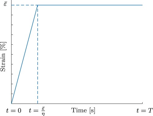
We consider relaxation experiments in which a strain is applied to a material. For a given strain rate η and maximum strain value $\overline{ϵ}$, the strain in a time interval $t\in [0,T]$ is given as (1) $ϵ\left(t\right)=\{\begin{array}{ll}\eta \cdot t,& 0\le t\le {\displaystyle \frac{\overline{ϵ}}{\eta }},\\ \overline{ϵ},& {\displaystyle \frac{\overline{ϵ}}{\eta }}<t\le T.\end{array}$(1) The function is illustrated in Figure 1 and describes the following procedure. The material is stretched until we reach a maximum strain value $\overline{ϵ}$ at a strain rate η, which can be calculated from the displacement rate ${\eta }_u$ and the specimen length $l_0$ as (2) $\eta ={\eta }_u\cdot l_0.$(2) The strain rate is known in the experiment by dividing the displacement rate given by the testing machine by the specimen length. The maximum strain is reached accordingly at time $t=\frac{\overline{ϵ}}{\eta }$. Afterwards the applied strain is kept constant.

Figure 1. Strain–time curve ε with strain rate η and maximum strain value $\overline{ϵ}$.

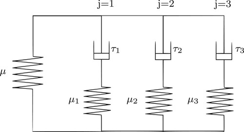
We describe the stress in the material by a rheological multi-parameter model combining a spring and several Maxwell elements to a generalized Maxwell model. Two opposing properties are essentially determining the time evolution of a material under strain, elasticity and viscosity. Elasticity is modelled by a spring, whereas viscosity is modelled by a damper. The series composition of a spring and a damper yields a Maxwell element. We use one of the most common combinations to represent the material, a parallel combination of a spring with different Maxwell elements [17,36,37]. A parallel combination of these elements ensures that the entire relaxation spectrum of the material can be represented by the model.

The number of Maxwell elements can extend to any number n with a relaxation time ${\tau }_j$ in each of the dampers and a stiffness of the spring ${\mu }_j$ in each of the Maxwell elements. In Figure 2 we see an illustration with three Maxwell elements. The deformation across the damper and across the spring in a Maxwell element changes according to the relaxation time of the damper. The Maxwell springs reach the original undeformed position and do not produce any stress after fully relaxing. Therefore, with a single Maxwell element the model can only simulate one stiffness for the entire duration of relaxation of the material. However, viscoelastic materials show different stiffnesses at different relaxation times [20,36] and, thus, a single element is not sufficient to describe viscoelastic behaviour appropriately. The entire relaxation spectrum can be divided into different regions such as the flow region, the entanglement region, the transition region and the glassy region [38]. The arrangement, the length and the entanglement of the polymeric chains on the molecular level explains the varying stiffness during the relaxation spectrum. A shorter chain relaxes faster than a longer chain and hence, after its relaxation, it does not contribute to the stiffness of the material [39]. Moreover, if all the Maxwell elements relax to zero stresses, then the equilibrium position is attained and the single spring with stiffness μ represents the basic stiffness of the material, which ensures that the material has a stiffness in its unperturbed position and does not behave like a fluid. The deformation of the material represented by the strain value ε is divided into an elastic component ${ϵ}_j^e$ and an inelastic component ${ϵ}_j^i$ in each of the Maxwell elements. The elastic component corresponds to the spring and the non-elastic component to the damper. As the stretching of the damper is dependent on its relaxation time, an evolution equation based on the energy conservation is used to model the change in the inelastic strain with time [40,41]. For small deformations the evolution equation is given by (3) ${\dot{ϵ}}_j^i\left(t\right)=\frac{ϵ\left(t\right)-{ϵ}_j^i\left(t\right)}{{\tau }_j/2},$(3) where ${\dot{ϵ}}_j^i$ represents the time derivative. The total stress produced in the system is then given by the sum of stresses induced in each of the springs. By assuming a linear elastic behaviour of the springs, the stress is given by (4) $\sigma \left(t\right)=\mu ϵ\left(t\right)+\sum _{j=1}^n{\mu }_j\left(ϵ\right(t)-{ϵ}_j^i(t\left)\right).$(4) With this information we have now all ingredients available to construct the forward operator as (5) $\begin{array}{rl}& F_n:{\mathbb{R}}_{\ge 0}^{2n+1}\times \mathbb{N}\to L^2\left(\right[0,T\left]\right),\end{array}$(5) (6) $\begin{array}{rl}& (\mu ,{\mu }_1,\dots ,{\mu }_n,{\tau }_1,\dots {\tau }_n,n)\mapsto \sigma ,\end{array}$(6) where n is the number of Maxwell elements and σ is the stress defined by Equation (4(4) $\sigma \left(t\right)=\mu ϵ\left(t\right)+\sum _{j=1}^n{\mu }_j\left(ϵ\right(t)-{ϵ}_j^i(t\left)\right).$(4) ). We note that the forward operator depends on parts of the solution at this point, since we require the unknown number of Maxwell elements n to calculate the stress. The number n is not defined and held fixed beforehand, but rather computed with the material parameters simultaneously. This is a novel setting in the field of inverse problems and different from the theory in classical textbooks such as [28]. We will address this problem in Section 4.

Figure 2. Rheological model with three Maxwell elements.

At this point, the inelastic stresses are included as a constraint in the formulation of the inverse problem. In the following section, we will see that these constraints can be directly included to obtain an explicit formulation of the forward operator.

3. Analytical solution of the forward problem and data simulation

For the solution of the forward problem, we first want to focus on the calculation of the inelastic component of the strain value ${ϵ}_j^i$, which is not explicitly given as a so-called internal variable of the system. An evolution equation such as (3(3) ${\dot{ϵ}}_j^i\left(t\right)=\frac{ϵ\left(t\right)-{ϵ}_j^i\left(t\right)}{{\tau }_j/2},$(3) ) is often solved by numerical methods like the Crank–Nicolson method. However, these methods have the disadvantage of approximation errors. Since we are dealing with an ill-posed inverse problem, it is desirable to avoid such errors in the calculation of the forward problem. To this end, we discuss the analytical solution of the evolution equation and, using this, the forward problem in the next section.

Apart from the mechanical application [41], the evolution equation (3(3) ${\dot{ϵ}}_j^i\left(t\right)=\frac{ϵ\left(t\right)-{ϵ}_j^i\left(t\right)}{{\tau }_j/2},$(3) ) is also used in other applications like Magnetic Particle Imaging [42] to model relaxation. Its solution can be formulated analytically as ${ϵ}_j^i\left(t\right)={\int }_0^tϵ\left(\tilde{t}\right)\frac{2}{{\tau }_j}\exp (-2\frac{t-\tilde{t}}{{\tau }_j})\mathrm{d}\tilde{t}.$By inserting the piecewise piecewise linear strain (1(1) $ϵ\left(t\right)=\{\begin{array}{ll}\eta \cdot t,& 0\le t\le {\displaystyle \frac{\overline{ϵ}}{\eta }},\\ \overline{ϵ},& {\displaystyle \frac{\overline{ϵ}}{\eta }}<t\le T.\end{array}$(1) ) we obtain the following result:

Proposition 3.1

The inelastic strain ${ϵ}_j^i$ of the jth Maxwell element with the corresponding relaxation time ${\tau }_j$ at time $t\in [0,T]$ is given by (7) ${ϵ}_j^i\left(t\right)=\{\begin{array}{ll}{\displaystyle \frac{{\tau }_j}{2}}\eta \exp (-{\displaystyle \frac{2}{{\tau }_j}}t)+\eta t-{\displaystyle \frac{{\tau }_j}{2}}\eta ,& 0\le t\le {\displaystyle \frac{\overline{ϵ}}{\eta }},\\ {\displaystyle \frac{{\tau }_j\eta }{2}}\exp (-{\displaystyle \frac{2}{{\tau }_j}}t)[1-\exp \left({\displaystyle \frac{2\overline{ϵ}}{{\tau }_j\eta }}\right)]+\overline{ϵ},& {\displaystyle \frac{\overline{ϵ}}{\eta }}<t\le T.\end{array}$(7)

Proof.

We first consider $0\le t\le \frac{\overline{ϵ}}{\eta }$ and can thus use $ϵ\left(t\right)=\eta t$, $\begin{array}{rl}{ϵ}_j^i\left(t\right)& =\frac{2}{{\tau }_j}\eta \exp (-\frac{2}{{\tau }_j}t){\int }_0^t\tilde{t}\exp \left(\frac{2}{{\tau }_j}\tilde{t}\right)\mathrm{d}\tilde{t}\\ & =\frac{2}{{\tau }_j}\eta \exp (-\frac{2}{{\tau }_j}t)\frac{{\tau }_j^2}{4}[\exp \left(\frac{2}{{\tau }_j}t\right)(\frac{2}{{\tau }_j}t-1)+1],\end{array}$where we used ${\int }_0^t\tilde{t}\exp \left(a\tilde{t}\right)\mathrm{d}\tilde{t}=\frac{1}{a^2}(\exp (at\left)\right(at-1)+1)$ for $a\in \mathbb{R}$ in the last step. The remainder is only a matter of transformation, $\begin{array}{rl}{ϵ}_j^i\left(t\right)& =\frac{{\tau }_j}{2}\eta \exp (-\frac{2}{{\tau }_j}t)\frac{2}{{\tau }_j}t\exp \left(\frac{2}{{\tau }_j}t\right)\\ & -\frac{{\tau }_j}{2}\eta \exp (-\frac{2}{{\tau }_j}t)\exp \left(\frac{2}{{\tau }_j}t\right)\\ & +\frac{{\tau }_j}{2}\eta \exp (-\frac{2}{{\tau }_j}t)\\ & =\frac{{\tau }_j}{2}\eta \exp (-\frac{2}{{\tau }_j}t)+\eta t-\frac{{\tau }_j}{2}\eta .\end{array}$Next we examine the case $\frac{\overline{ϵ}}{\eta }<t\le T$, where we have to split the integral into two parts to be able to use the corresponding value for $ϵ\left(t\right)$, ${ϵ}_j^i\left(t\right)=\frac{2}{{\tau }_j}\exp (-\frac{2}{{\tau }_j}t)[\eta {\int }_0^{\frac{\overline{ϵ}}{\eta }}\tilde{t}\exp \left(\frac{2}{{\tau }_j}\tilde{t}\right)\mathrm{d}\tilde{t}+\overline{ϵ}{\int }_{\frac{\overline{ϵ}}{\eta }}^t\exp \left(\frac{2}{{\tau }_j}\tilde{t}\right)\mathrm{d}\tilde{t}].$For each integral we then get $\begin{array}{rl}& {\int }_0^{\frac{\overline{ϵ}}{\eta }}\tilde{t}\exp \left(\frac{2}{{\tau }_j}\tilde{t}\right)\mathrm{d}\tilde{t}=\frac{{\tau }_j^2}{4}[\exp \left(\frac{2\overline{ϵ}}{{\tau }_j\eta }\right)(\frac{2\overline{ϵ}}{{\tau }_j\eta }-1)+1],\\ & {\int }_{\frac{\overline{ϵ}}{\eta }}^t\exp \left(\frac{2}{{\tau }_j}\tilde{t}\right)\mathrm{d}\tilde{t}=\frac{{\tau }_j}{2}[\exp \left(\frac{2}{{\tau }_j}t\right)-\exp \left(\frac{2\overline{ϵ}}{{\tau }_j\eta }\right)].\end{array}$Inserting these results yields $\begin{array}{rl}{ϵ}_j^i\left(t\right)& =\frac{2}{{\tau }_j}\exp (-\frac{2}{{\tau }_j}t)[\eta \frac{{\tau }_j^2}{4}[\exp \left(\frac{2\overline{ϵ}}{{\tau }_j\eta }\right)(\frac{2\overline{ϵ}}{{\tau }_j\eta }-1)+1]\\ & +\overline{ϵ}\frac{{\tau }_j}{2}[\exp \left(\frac{2}{{\tau }_j}t\right)-\exp \left(\frac{2\overline{ϵ}}{{\tau }_j\eta }\right)]\phantom{\frac{{\tau }_j^2}{4}}]\\ & =\frac{2}{{\tau }_j}\exp (-\frac{2}{{\tau }_j}t)\\ & \times [\eta \frac{{\tau }_j^2}{4}\frac{2\overline{ϵ}}{{\tau }_j\eta }\exp \left(\frac{2\overline{ϵ}}{{\tau }_j\eta }\right)-\eta \frac{{\tau }_j^2}{4}\exp \left(\frac{2\overline{ϵ}}{{\tau }_j\eta }\right)+\eta \frac{{\tau }_j^2}{4}\\ & +\overline{ϵ}\frac{{\tau }_j}{2}\exp \left(\frac{2}{{\tau }_j}t\right)-\overline{ϵ}\frac{{\tau }_j}{2}\exp \left(\frac{2\overline{ϵ}}{{\tau }_j\eta }\right)]\\ & =\exp (-\frac{2}{{\tau }_{j}t})[\exp \left(\frac{2\overline{ϵ}}{{\tau }_j\eta }\right)(\overline{ϵ}-\frac{{\tau }_j\eta }{2}-\overline{ϵ})+\frac{{\tau }_j\eta }{2}+\exp \left(\frac{2}{{\tau }_{j}t}\right)\overline{ϵ}]\\ & =-\frac{{\tau }_j\eta }{2}\exp (-\frac{2}{{\tau }_j}t+\frac{2\overline{ϵ}}{{\tau }_j\eta })+\frac{{\tau }_j\eta }{2}\exp (-\frac{2}{{\tau }_j}t)+\overline{ϵ}\\ & =\frac{{\tau }_j\eta }{2}\exp (-\frac{2}{{\tau }_j}t)[1-\exp \left(\frac{2\overline{ϵ}}{{\tau }_j\eta }\right)]+\overline{ϵ}.\text{■}\end{array}$

We use this result to obtain the stress responses of the individual Maxwell elements. This is also useful for an analysis of different strain rates η and displacement rate ${\eta }_u$, respectively in Section 5.3.

Proposition 3.2

The stress ${\sigma }_j$ of the jth Maxwell element with j>1 and the corresponding stiffness ${\mu }_j$ and relaxation time ${\tau }_j$ at time $t\in [0,T]$ are given as (8) ${\sigma }_j\left(t\right)=\{\begin{array}{ll}{\displaystyle \frac{{\mu }_j{\tau }_j\eta }{2}}(1-\exp (-{\displaystyle \frac{2}{{\tau }_j}}t)),& 0\le t\le {\displaystyle \frac{\overline{ϵ}}{\eta }},\\ -{\displaystyle \frac{{\mu }_j{\tau }_j\eta }{2}}(1-\exp \left({\displaystyle \frac{2\overline{ϵ}}{{\tau }_j\eta }}\right))\exp (-{\displaystyle \frac{2}{{\tau }_j}}t),& {\displaystyle \frac{\overline{ϵ}}{\eta }}<t\le T.\end{array}$(8) The stress of the single spring, denoted by ${\sigma }_0$, can be specified with the corresponding stiffness μ as (9) ${\sigma }_0\left(t\right)=\{\begin{array}{ll}\mu \eta t,& 0\le t\le {\displaystyle \frac{\overline{ϵ}}{\eta }},\\ \mu \overline{ϵ},& {\displaystyle \frac{\overline{ϵ}}{\eta }}<t\le T.\end{array}$(9) According to these calculations, the total stress can be written as the sum of the stresses of the single spring and the Maxwell elements, i.e. (10) $\sigma \left(t\right)=\sum _{j=0}^n{\sigma }_j\left(t\right)=\{\begin{array}{ll}\mu \eta t+\sum _{j=1}^n{\displaystyle \frac{{\mu }_j{\tau }_j\eta }{2}}(1-\exp (-{\displaystyle \frac{2}{{\tau }_j}}t)),& 0\le t\le {\displaystyle \frac{\overline{ϵ}}{\eta }},\\ \mu \overline{ϵ}-\sum _{j=1}^n{\displaystyle \frac{{\mu }_j{\tau }_j\eta }{2}}(1-\exp \left({\displaystyle \frac{2\overline{ϵ}}{{\tau }_j\eta }}\right))\exp (-{\displaystyle \frac{2}{{\tau }_j}}t),& {\displaystyle \frac{\overline{ϵ}}{\eta }}<t\le T.\end{array}$(10)

Proof.

We start with the stress of the single spring. This is calculated by ${\sigma }_0\left(t\right)=\mu ϵ\left(t\right)$. Inserting (1(1) $ϵ\left(t\right)=\{\begin{array}{ll}\eta \cdot t,& 0\le t\le {\displaystyle \frac{\overline{ϵ}}{\eta }},\\ \overline{ϵ},& {\displaystyle \frac{\overline{ϵ}}{\eta }}<t\le T.\end{array}$(1) ) for the different time intervals yields (9(9) ${\sigma }_0\left(t\right)=\{\begin{array}{ll}\mu \eta t,& 0\le t\le {\displaystyle \frac{\overline{ϵ}}{\eta }},\\ \mu \overline{ϵ},& {\displaystyle \frac{\overline{ϵ}}{\eta }}<t\le T.\end{array}$(9) ). The stress of the Maxwell elements is calculated by ${\sigma }_j\left(t\right)={\mu }_j\left(ϵ\right(t)-{ϵ}_j^i(t\left)\right)$ as given in Equation (4(4) $\sigma \left(t\right)=\mu ϵ\left(t\right)+\sum _{j=1}^n{\mu }_j\left(ϵ\right(t)-{ϵ}_j^i(t\left)\right).$(4) ). By considering the different time intervals we can insert both the strain $ϵ\left(t\right)$ and the inelastic strain ${ϵ}_j^i\left(t\right)$ of the Maxwell element. Hence, for $0\le t\le \frac{\overline{ϵ}}{\eta }$ we obtain ${\sigma }_j\left(t\right)={\mu }_j(\eta t-\frac{{\tau }_j}{2}\eta \exp (-\frac{2}{{\tau }_j}t)-\eta t+\frac{{\tau }_j}{2}\eta )=\frac{{\mu }_j{\tau }_j\eta }{2}(1-\exp (-\frac{2}{{\tau }_j}t)).$Similarly, for $\frac{\overline{ϵ}}{\eta }<t\le T$, we obtain $\begin{array}{rl}{\sigma }_j\left(t\right)& ={\mu }_j(\overline{ϵ}-\frac{{\tau }_j\eta }{2}\exp (-\frac{2}{{\tau }_j}t)[1-\exp \left(\frac{2\overline{ϵ}}{{\tau }_j\eta }\right)]-\overline{ϵ})\\ & =-\frac{{\mu }_j{\tau }_j\eta }{2}(1-\exp \left(\frac{2\overline{ϵ}}{{\tau }_j\eta }\right))\exp (-\frac{2}{{\tau }_j}t).\end{array}$The representation of the total stress (10(10) $\sigma \left(t\right)=\sum _{j=0}^n{\sigma }_j\left(t\right)=\{\begin{array}{ll}\mu \eta t+\sum _{j=1}^n{\displaystyle \frac{{\mu }_j{\tau }_j\eta }{2}}(1-\exp (-{\displaystyle \frac{2}{{\tau }_j}}t)),& 0\le t\le {\displaystyle \frac{\overline{ϵ}}{\eta }},\\ \mu \overline{ϵ}-\sum _{j=1}^n{\displaystyle \frac{{\mu }_j{\tau }_j\eta }{2}}(1-\exp \left({\displaystyle \frac{2\overline{ϵ}}{{\tau }_j\eta }}\right))\exp (-{\displaystyle \frac{2}{{\tau }_j}}t),& {\displaystyle \frac{\overline{ϵ}}{\eta }}<t\le T.\end{array}$(10) ) follows directly by inserting (8(8) ${\sigma }_j\left(t\right)=\{\begin{array}{ll}{\displaystyle \frac{{\mu }_j{\tau }_j\eta }{2}}(1-\exp (-{\displaystyle \frac{2}{{\tau }_j}}t)),& 0\le t\le {\displaystyle \frac{\overline{ϵ}}{\eta }},\\ -{\displaystyle \frac{{\mu }_j{\tau }_j\eta }{2}}(1-\exp \left({\displaystyle \frac{2\overline{ϵ}}{{\tau }_j\eta }}\right))\exp (-{\displaystyle \frac{2}{{\tau }_j}}t),& {\displaystyle \frac{\overline{ϵ}}{\eta }}<t\le T.\end{array}$(8) ) in (4(4) $\sigma \left(t\right)=\mu ϵ\left(t\right)+\sum _{j=1}^n{\mu }_j\left(ϵ\right(t)-{ϵ}_j^i(t\left)\right).$(4) ).

Since the stress can be expressed in terms of the material parameters, we are able to formulate the forward operator (5(5) $\begin{array}{rl}& F_n:{\mathbb{R}}_{\ge 0}^{2n+1}\times \mathbb{N}\to L^2\left(\right[0,T\left]\right),\end{array}$(5) ), which is still depending on parts of the solution, because the number of Maxwell elements is unknown. Before we address this topic, we will briefly discuss the simulation of data, where the above results prove to be helpful.

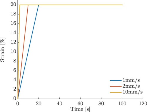
We simulate a relaxation experiment where a strain is applied to a material. This strain is completely determined by the parameters ${\eta }_u$ (displacement rate), $l_0$ (specimen length) and $\overline{ϵ}$ (maximum strain). Since all specimens are of equal length, the displacement rate ${\eta }_u$ instead of the strain rate η is used in the following. So, if we define the above three parameters and a time period $[0,T]$, we have completely determined the strain using the representation (1(1) $ϵ\left(t\right)=\{\begin{array}{ll}\eta \cdot t,& 0\le t\le {\displaystyle \frac{\overline{ϵ}}{\eta }},\\ \overline{ϵ},& {\displaystyle \frac{\overline{ϵ}}{\eta }}<t\le T.\end{array}$(1) ). This function can then be supposed to be known for all $t\in [0,T]$. In Figure 3, we see strains for three different displacement rates ${\eta }_u$ and the maximum strain $\overline{ϵ}=20\mathrm{\%}$. The fastest displacement rate is 10 mm/s with a maximum strain being attained after 2 s. For the slowest displacement rate of 1 mm/s, the $20\mathrm{\%}$ strain is only achieved after 20 s. We chose T = 100 s.

Figure 3. Strain–time curves for different displacement rates ${\eta }_u$.

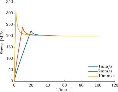
For the simulation of the stress function we then choose the number of Maxwell elements n and the material parameters $(\mu ,{\mu }_1,\dots ,{\mu }_n,{\tau }_1,\dots {\tau }_n)$. Thus, we can solve the forward problem with Equation (10(10) $\sigma \left(t\right)=\sum _{j=0}^n{\sigma }_j\left(t\right)=\{\begin{array}{ll}\mu \eta t+\sum _{j=1}^n{\displaystyle \frac{{\mu }_j{\tau }_j\eta }{2}}(1-\exp (-{\displaystyle \frac{2}{{\tau }_j}}t)),& 0\le t\le {\displaystyle \frac{\overline{ϵ}}{\eta }},\\ \mu \overline{ϵ}-\sum _{j=1}^n{\displaystyle \frac{{\mu }_j{\tau }_j\eta }{2}}(1-\exp \left({\displaystyle \frac{2\overline{ϵ}}{{\tau }_j\eta }}\right))\exp (-{\displaystyle \frac{2}{{\tau }_j}}t),& {\displaystyle \frac{\overline{ϵ}}{\eta }}<t\le T.\end{array}$(10) ) obtaining the stress function σ. In Figure 4 we see the stress functions corresponding to the strains with different displacement rates ${\eta }_u$ of Figure 3. Here, we have selected one spring and three Maxwell elements with the material parameters $\mu =10$, $({\mu }_1,{\tau }_1)=(4,0.2)$, $({\mu }_2,{\tau }_2)=(7,3.7)$ and $({\mu }_3,{\tau }_3)=(1,25)$. The stiffnesses μ and ${\mu }_j$ have the unit MPa and the unit of the relaxation times of the different dampers are seconds. The relaxation times were selected in three different decades to simulate a relaxation time spectrum, whereas the stiffness for each of the elements were selected randomly to ensure no correlation between the relaxation time and the stiffness. Since the Maxwell elements are connected in parallel in the rheological model as shown in Figure 2, the order of the Maxwell elements is not important. This is also evident in the forward model (10(10) $\sigma \left(t\right)=\sum _{j=0}^n{\sigma }_j\left(t\right)=\{\begin{array}{ll}\mu \eta t+\sum _{j=1}^n{\displaystyle \frac{{\mu }_j{\tau }_j\eta }{2}}(1-\exp (-{\displaystyle \frac{2}{{\tau }_j}}t)),& 0\le t\le {\displaystyle \frac{\overline{ϵ}}{\eta }},\\ \mu \overline{ϵ}-\sum _{j=1}^n{\displaystyle \frac{{\mu }_j{\tau }_j\eta }{2}}(1-\exp \left({\displaystyle \frac{2\overline{ϵ}}{{\tau }_j\eta }}\right))\exp (-{\displaystyle \frac{2}{{\tau }_j}}t),& {\displaystyle \frac{\overline{ϵ}}{\eta }}<t\le T.\end{array}$(10) ), since we simply have a sum of the stress contributions of the individual Maxwell elements and the single spring. So we stick to the convention to always number them according to the order of the relaxation times.

Figure 4. Synthetic stress–time data produced by a model consisting of a spring combined with three Maxwell elements for three different displacement rates.

For the calculation of σ we have to discretize with respect to time. We choose m + 1 as the number of time steps $t_i=i\cdot \frac{T}{m}$ for $i=0,\dots ,m$ in the interval $[0,T]$ and thus also have a discretized representation of the stress function with $\left(\sigma \right(t_0),\dots ,\sigma (t_m\left)\right)\in {\mathbb{R}}^{m+1}$. When inverting synthetic data one has to avoid the same discretization for simulating the data and the inversion process, since otherwise the numerical results can be highly accurate and pretend a quality of the algorithm that is not apparent for noisy data. This phenomenon was first characterized by Colton and Kress [43] and is meanwhile known as inverse crime. Hence, to avoid an inverse crime, one has to choose a different discretization for the direct and inverse problems. But since we can analytically compute the forward problem depending on the number of Maxwell elements n, this problem is avoided in our situation. In Section 5 we discuss results of experiments and show various scenarios that lead to the reconstructions of different accuracy concerning the material parameters.

For any ill-posed inverse problem, reconstruction is considerably more difficult in case of noisy data ${\sigma }^{\delta }$. In this regard, we will also see different results in Section 5. We simulate noise by adding scaled standard normally distributed random numbers to the discretized stress vector such that $\Vert \sigma -{\sigma }^{\delta }\Vert <\delta$ with noise level $\delta >0$. A noise level $\delta =0$ corresponds to unperturbed (exact) data.

4. Solving the inverse problem

In this section we develop a novel clustering algorithm, by which we overcome the mentioned fact that the forward operator depends on the unknown number of Maxwell elements. Currently, we cannot compute the forward operator without a fixed number of Maxwell elements. Together with the ambiguity of our forward operator, this contributes to the ill-posedness of the problem. To illustrate the mentioned ambiguity, we consider the following example.

Example 4.1

For a material described by two Maxwell elements with relaxation times ${\tau }_1={\tau }_2$ and stiffnesses ${\mu }_1,{\mu }_2$ we have ${ϵ}_1^i={ϵ}_2^i$. We furthermore consider another material described by the same basic stiffness but only one Maxwell element with relaxation time $\widetilde{{\tau }_1}={\tau }_1={\tau }_2$ and stiffness $\widetilde{{\mu }_1}$. If additionally $\widetilde{{\mu }_1}={\mu }_1+{\mu }_2$ applies, there is no possibility to distinguish these two materials by means of the stress created by our forward operator. The two stress–time curves are exactly the same with no possibility to reconstruct the parameters unambiguously.

This shows how to construct different tuples $(\mu ,{\mu }_1,\dots ,{\mu }_n,{\tau }_1,\dots ,{\tau }_n,n)$, such that $F_n(\mu ,{\mu }_1,\dots ,{\mu }_n,{\tau }_1,\dots {\tau }_n,n)=\sigma$for a specific $\sigma \in L_2\left(\right[0,T\left]\right)$, what means that the forward operator is not injective. For this reason we make further requirements. A common assumption is that the occurring relaxation times lie in different decades [44]. For instance, if ${\tau }_l\in [10,100]$ for $l\in \{1,\dots ,N\}$, then ${\tau }_j\notin [10,100]$ for all $j\in \{1,\dots ,l-1,l+1,\dots N\}$. This information will help us to solve the ill-posed problem.

We set a maximum number of Maxwell elements N, such that the unknown actual number of Maxwell elements n is smaller or equal to N. Then, we reconstruct the desired parameters $(\mu ,{\mu }_1,\dots ,{\mu }_N,{\tau }_1,\dots {\tau }_N)$ with a minimization algorithm, obtaining the stiffness parameter for the single spring as well as stiffnesses and relaxation times for N Maxwell elements. Of course, at this point there could be too many parameters, because the number of Maxwell elements could be too large. Nevertheless these values are helpful. They do not fulfill the requirement of having the relaxation times in different decades yet. Therefore, we apply a clustering algorithm to these parameters, which clusters them according to this requirement. That means our reconstruction consists of two parts:

• minimization algorithm with N Maxwell elements,

• clustering algorithm which reduces N to n Maxwell elements.

We describe this in more detail.

The first step consists of minimizing the residual (11) $R=\Vert F_N(\mu ,{\mu }_1,\dots ,{\mu }_N,{\tau }_1,\dots {\tau }_N,N)-\sigma {\Vert }_2^2$(11) with respect to $(\mu ,{\mu }_1,\dots ,{\mu }_N,{\tau }_1,\dots {\tau }_N)$ under the assumption to have N Maxwell elements. Since the problem is nonlinear with respect to the relaxation times, there exist, in general, several local minima. This is why we use an iterative solution method with several starting values for the stiffnesses and relaxation times $({\mu }^{\left(0\right)},{\mu }_1^{\left(0\right)},\dots ,{\mu }_N^{\left(0\right)},{\tau }_1^{\left(0\right)},\dots {\tau }_N^{\left(0\right)})$. The starting values are distributed over the entire possible range of parameter values and re-defined in each iteration step. As solver we use the function lsqnonlin and MultiStart provided in the MATLAB Optimization Toolbox [45]. Here, the iteration number in lsqnonlin acts as a regularization number.

The next step consists of clustering parameters with relaxation times contained in the same decade. For a decade $[{10}^k,{10}^{k+1}]$, $k\in \mathbb{N}$, we consider the index set $J_k:=\{j\in \{1,\dots ,N\}:{\tau }_j\in [{10}^k,{10}^{k+1}\left]\right\}.$Of course, depending on the application, other intervals instead of decades can also be of interest. All pairs $({\mu }_j,{\tau }_j)$, $j\in J_k$, are assigned to the same Maxwell element leading to a number of $n\le N$ Maxwell elements. After the clustering we calculate new parameters $({\tilde{\mu }}_k,{\tilde{\tau }}_k)$ with ${\tilde{\tau }}_k\in [{10}^k,{10}^{k+1}]$ from the already reconstructed parameters by (12) ${\tilde{\mu }}_k:=\sum _{j\in J_k}{\mu }_j,{\tilde{\tau }}_k:=\sum _{j\in J_k}\frac{{\mu }_j}{{\tilde{\mu }}_k}{\tau }_j$(12) and in this way avoid to start again an elaborate minimization process.

The cluster algorithm finally can be summarized as follows.

Example 4.2

We look at different cases and how they are treated by the clustering algorithm.

1. Let, for some $k\in \mathbb{N}$, $J_k=\{1,3,5\}$ with ${\tau }_1={\tau }_3={\tau }_5$ and N = 6. It is obvious that this should actually be a single Maxwell element. Consider the forward operator with $\sigma \left(t\right)=\mu ϵ\left(t\right)+\sum _{j=1}^N{\mu }_j(ϵ\left(t\right)-{ϵ}_j^i\left(t\right)).$Since ${ϵ}_j^i$ varies only in ${\tau }_j$ for different Maxwell elements, it follows that ${ϵ}_1^i={ϵ}_3^i={ϵ}_5^i$ leading to (13) $\sigma \left(t\right)=\mu ϵ\left(t\right)+({\mu }_1+{\mu }_3+{\mu }_5)\left(ϵ\right(t)-{ϵ}_1^i(t\left)\right)+\sum _{j=2,4,6}{\mu }_j\left(ϵ\right(t)-{ϵ}_j^i(t\left)\right).$(13) Therefore, it is reasonable to choose the new values as $({\tilde{\mu }}_k,{\tilde{\tau }}_k)=({\mu }_1+{\mu }_3+{\mu }_5,{\tau }_1).$This is in fact the result of the clustering step, since $\begin{array}{rl}{\tilde{\mu }}_k& =\sum _{j\in J_k}{\mu }_j={\mu }_1+{\mu }_3+{\mu }_5,\\ {\tilde{\tau }}_k& =\sum _{j\in J_k}\frac{{\mu }_j}{{\tilde{\mu }}_k}{\tau }_j=\frac{{\mu }_1+{\mu }_3+{\mu }_5}{{\mu }_1+{\mu }_3+{\mu }_5}{\tau }_1={\tau }_1.\end{array}$

2. In the next case we want to illustrate the calculation of the relaxation times in the clustering algorithm. Let $J_k=\{1,3,5\}$ with $({\mu }_1,{\tau }_1)=(7,4)$, $({\mu }_3,{\tau }_3)=(1,4.5)$ and $({\mu }_5,{\tau }_5)=(2,3.75)$, i.e. ${\tau }_1\approx {\tau }_3\approx {\tau }_5$. Then the stiffness values serve as a weighting of how important the corresponding relaxation value is. Regarding the forward operator (13(13) $\sigma \left(t\right)=\mu ϵ\left(t\right)+({\mu }_1+{\mu }_3+{\mu }_5)\left(ϵ\right(t)-{ϵ}_1^i(t\left)\right)+\sum _{j=2,4,6}{\mu }_j\left(ϵ\right(t)-{ϵ}_j^i(t\left)\right).$(13) ) we observe that, under these assumptions, the values of $ϵ\left(t\right)-{ϵ}_j^i\left(t\right)$, $t\in [0,T]$, for j = 1, 3, 5 are quite similar, especially considering that other relaxation times lie in different decades. Thus, if one assumes that ${ϵ}_1^i\approx {ϵ}_3^i\approx {ϵ}_5^i$ applies, we see that the largest contribution among these three to the total stress is provided by the Maxwell element $({\mu }_1,{\tau }_1)$, since ${\mu }_1\gg {\mu }_5>{\mu }_3$. In order to include this weighting in more complicated examples, the clustering algorithm calculates ${\tilde{\tau }}_k$ as follows, instead of just calculating the mean value of all relaxation times, $\begin{array}{rl}{\tilde{\mu }}_k& =\sum _{j\in J_k}{\mu }_j={\mu }_1+{\mu }_2+{\mu }_3=10,\\ {\tilde{\tau }}_k& =\sum _{j\in J_k}\frac{{\mu }_j}{{\tilde{\mu }}_k}{\tau }_j=\frac{7}{10}\cdot 4+\frac{1}{10}\cdot 4.5+\frac{2}{10}\cdot 3.75=4.\end{array}$

Remark 4.1

We mention that it is not possible to compute the exact number of Maxwell elements n, if we choose an initial guess N<n. This is inherent by the construction of the algorithm. So, it is always favourable to overestimate the number of elements. Then the algorithm shows a good performance as is demonstrated in Section 5.

5. Numerical results

In this section we show numerical results of our derived minimization and clustering algorithm. For the evaluation of our method we generate simulated data for known material parameters that serve as ground truth. We choose a material described by one spring for basic elasticity and n = 3 Maxwell elements and the following material parameters:

By solving the forward operator analytically (see Proposition 3.2) we obtain the stress–time curve of the material, which we observe in the range $[0,100]$ seconds. The parameters from Table 1 are to be reconstructed in all the experiments. We discuss the difference between reconstructions from perturbed as well as exact data, different displacement rates and their effects. Finally, we consider regularization, which is indispensable for perturbed data.

Table 1. Selected material parameters to simulate data.

j	0	1	2	3
${\mu }_j$ [MPa]	10	4	7	1
${\tau }_j$ [s]	–	0.2	3.7	25

5.1. Exact data

We will see that in case of exact data we can determine the material parameters very reliably. Table 2 shows the effects of the clustering algorithm. While the minimization algorithm determines stiffnesses and relaxation times for the given maximum number of Maxwell elements (here N = 5), the clustering algorithm can combine them accordingly and thus obtain the actual number n = 3. Here, we used the complete data set for $t\in [0,100]$ seconds and a displacement rate of 1 mm/s, see Figure 3.

Table 2. Reconstructed material parameters before and after clustering where the ${\mu }_j$ are given in MPa and the ${\tau }_j$ in seconds.

$j=$	0	1	2	3	4	5
Reconstructed values
${\mu }_j$	10.000	4.000	3.685	1.621	1.694	1.000
${\tau }_j$	–	0.200	3.695	3.706	3.706	25.000
After clustering
${\mu }_j$	10.000	4.000	7.000	1.000
${\tau }_j$	–	0.200	3.700	25.000

While after the calculation of the minimization algorithm there is only one Maxwell element with $\tau \in [0,1)$ and $\tau \in [10,100)$, we have three Maxwell elements with associated relaxation times in $[1,10)$. The clustering algorithm merges these elements and we can see that our reconstruction is accurate. The values in the table are rounded to three decimal places. After this we no longer see any difference to the exact parameters after applying the clustering algorithm, see Table 1. We illustrate what we have already mentioned in the second part of Example 4.2. The relaxation time ${\tau }_2=3.695$ is closest to the current value of 3.7 before clustering and we have ${\mu }_2\gg {\mu }_4>{\mu }_3$, which allows the clustering algorithm to use the weighting (12(12) ${\tilde{\mu }}_k:=\sum _{j\in J_k}{\mu }_j,{\tilde{\tau }}_k:=\sum _{j\in J_k}\frac{{\mu }_j}{{\tilde{\mu }}_k}{\tau }_j$(12) ) leading to better results.

5.2. Perturbed data

We continue by investigating noisy data ${\sigma }^{\delta }$. These are generated by adding scaled standard normally distributed numbers to our discretized stress vector σ, such that $\Vert \sigma -{\sigma }^{\delta }\Vert <\delta$ with noise level $\delta >0$. We specify the relative noise level ${\delta }_{rel}$ by $\frac{\Vert \sigma -{\sigma }^{\delta }\Vert }{\Vert {\sigma }^{\delta }\Vert }<{\delta }_{rel}.$In our calculations we use the Euclidean norm and ${\delta }_{rel}\approx 1\mathrm{\%}$. Table 3 shows different results of a reconstruction at a displacement rate of 10 mm/s using the clustering algorithm with N = 5. To better assess the effect of the disturbance, we used several data sets for this purpose. That is, we have the same relative noise level ${\delta }_{rel}$, but different random numbers, which leads to slightly different data sets. We perform our reconstruction for each of these different data sets to identify possible weaknesses.

Table 3. Approximated material parameters with similar noisy data, where the ${\mu }_j$ are given in MPa and the ${\tau }_j$ in seconds.

$j=$		0	1	2	3
Exact values	${\mu }_j$	10	4	7	1
	${\tau }_j$	–	0.2	3.7	25
Experiment 1	${\mu }_j$	9.9951	38.558	7.2098	0.88371
	${\tau }_j$	–	0.019903	3.7734	27.795
Experiment 2	${\mu }_j$	10.005	2.475	6.9957	1.0157
	${\tau }_j$	–	0.29222	3.6908	24.2965
Experiment 3	${\mu }_j$	9.99348	44.351	7.2084	0.96407
	${\tau }_j$	–	0.01344	3.6444	26.633
Experiment 4	${\mu }_j$	10.003	7.3458	7.0398	0.99887
	${\tau }_j$	–	0.0993	3.6626	24.0342

We see that the reconstruction results differ, as expected, significantly from the exact values. However, it is obvious that the reconstructions of $({\mu }_1,{\tau }_1)$ show a tremendous error, while the other parameters are computed rather stably. This confirms considerations of the authors in [23] where it has been proven that the reconstruction of small relaxation times always is severely ill-conditioned and the condition deteriorates as $\tau \to 0$. Since stiffness and relaxation time are always to be considered in pairs, we see deviations in ${\tau }_1$ also in the corresponding stiffness ${\mu }_1$. As each Maxwell element has to provide a certain part to the total stress, too small values in one parameter are compensated by higher values in the other parameter to approach the total stress.

We repeat this experiment with 100 different perturbed data sets with the same noise level and plot the values of $({\mu }_1,{\tau }_1)$ in Figure 5. We see that there is a very large variance in values spread over 100 different experiments. The values are distributed up to results such as $({\mu }_1,{\tau }_1)=(66.75,0.0127)$ or $({\mu }_1,{\tau }_1)=(1.934,0.7992)$. Of course, there are also results that come close to the exact values. The median of all values is $(0.1897,4.0135)$, which is not far from the exact values. Figure 5 also shows that stiffness and relaxation time are inversely proportional to each other. If the relaxation time is estimated too small, we obtain much too large values for the stiffness. Similarly, if the relaxation time is too large, the stiffness is reconstructed too small.

Figure 5. Spread of the material parameters $({\mu }_1,{\tau }_1)$ for 100 runs with different noise seeds, but same noise level ${\delta }_{rel}$ for ${\eta }_u$ = 10 mm/s.

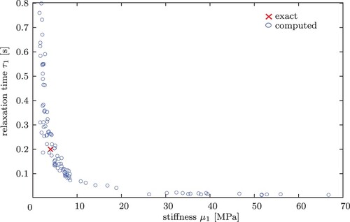
We summarize that the reconstruction from noisy data is, as expected, much worse in comparison to the results obtained for exact data. In particular, the Maxwell element with the smallest relaxation time (here: $({\mu }_1,{\tau }_1)$) is most affected. This confirms stability investigations obtained in [23].

5.3. Analysis of different displacement rates

So far we focused on experiments with the fastest displacement rate of 10 mm/s. In this subsection we discuss slower displacement rates.

We compare Table 3 with Table 4, in which we used a displacement rate of 10  and 1 mm/s, respectively. Again, we use N = 5 for the minimization and a relative noise level of about 1%, but four different noise seeds. It is obvious that the results are much worse, specifically the smallest relaxation time and the corresponding stiffness are approximated poorly. Again, this has to be expected since the reconstruction of small relaxation times is severely ill-conditioned. In a second run, the algorithm was not even able to find Maxwell elements with relaxation times in three different decades.

Table 4. Clustered material parameters with noisy data ($\eta =1$ mm/s) where the ${\mu }_j$ are given in MPa and the ${\tau }_j$ in seconds.

$j=$		0	1	2	3
Exact values	${\mu }_j$	10	4	7	1
	${\tau }_j$	–	0.2	3.7	25
Experiment 1	${\mu }_j$	9.9945	27.367	5.945	0.91663
	${\tau }_j$	–	0.088687	4.2318	27.263
Experiment 2	${\mu }_j$	10.007	–	7.5694	1.0434
	${\tau }_j$	–	–	3.4762	23.689
Experiment 3	${\mu }_j$	9.0111	2.6942	7.2928	1.0402
	${\tau }_j$	–	0.82841	6.3049	3000.5
Experiment 4	${\mu }_j$	10.006	2.094	6.0643	1.0303
	${\tau }_j$	–	0.885029	3.9963	23.423

For a better understanding of why the results are worse compared to the results for the faster displacement rate of 10 mm/s, we look at the different stress-time curves that a displacement rate of 1 mm/s Figure 6 and 10 mm/s Figure 7 generate. For each of the curves, we show the contribution of each element separately. That means ${\sigma }_0$ is the stress generated by the single spring while ${\sigma }_{1,2,3}$ is the stress of the three Maxwell elements. The sum of these individual stresses yields the total stress, cf. (10(10) $\sigma \left(t\right)=\sum _{j=0}^n{\sigma }_j\left(t\right)=\{\begin{array}{ll}\mu \eta t+\sum _{j=1}^n{\displaystyle \frac{{\mu }_j{\tau }_j\eta }{2}}(1-\exp (-{\displaystyle \frac{2}{{\tau }_j}}t)),& 0\le t\le {\displaystyle \frac{\overline{ϵ}}{\eta }},\\ \mu \overline{ϵ}-\sum _{j=1}^n{\displaystyle \frac{{\mu }_j{\tau }_j\eta }{2}}(1-\exp \left({\displaystyle \frac{2\overline{ϵ}}{{\tau }_j\eta }}\right))\exp (-{\displaystyle \frac{2}{{\tau }_j}}t),& {\displaystyle \frac{\overline{ϵ}}{\eta }}<t\le T.\end{array}$(10) ). The maximum strain is 20 $\mathrm{\%}$, which is attained at 20 and 2  s for a displacement rate of 1 and 10 mm/s, respectively. This makes a big difference for the individual stresses of the Maxwell elements. In both cases the maximum stress of the single spring is achieved at 200 MPa, but at different time instances. However, the maximum stress of the Maxwell elements at a slower displacement rate of 1 mm/s is much lower than for a faster displacement rate. In both cases, the maximum is attained at $t=\overline{ϵ}/\eta$. In Table 5, we see the different values listed. At a slower displacement rate, the stress values of the Maxwell elements are non-zero over a longer time period, which can be seen particularly well for the first Maxwell element. But since the values are so much smaller than at a higher displacement rate, these small values are covered by noise much more easily. Therefore, it is advisable to use higher displacement rates. Based on this, we confine to a displacement rate of 10 mm/s in upcoming examples.

Figure 6. Individual stress components for a displacement rate of 1 mm/s.

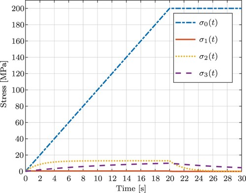
Figure 7. Individual stress components for a displacement rate of 10 mm/s.

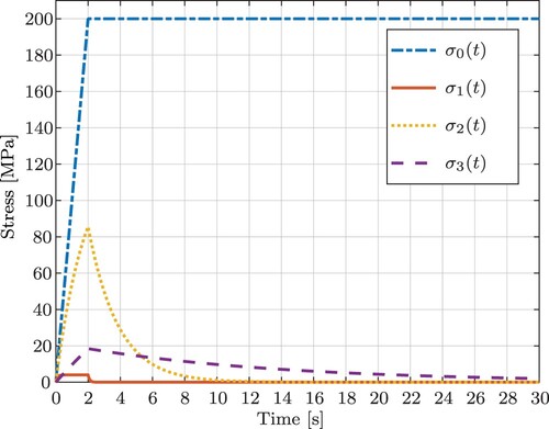
Table 5. Maximum values of individual stress components (MPa) with slow and fast deformation rates attained at $t=\overline{ϵ}/\eta$.

		j = 1	j = 2	j = 3
$\eta =1$	${\sigma }_j\left(\overline{ϵ}/\eta \right)$	0.4	12.94	9.9
$\eta =10$	${\sigma }_j\left(\overline{ϵ}/\eta \right)$	4	85.57	18.48

5.4. Regularization approaches

As a result of our investigations in Section 5.2 we realized that small errors in the data can lead to large errors in the solution. This is a typical behaviour of ill-posed inverse problems, which must be compensated by means of regularization techniques. Therefore, instead of continuing to use as cost function the residual (11(11) $R=\Vert F_N(\mu ,{\mu }_1,\dots ,{\mu }_N,{\tau }_1,\dots {\tau }_N,N)-\sigma {\Vert }_2^2$(11) ) only, we will add a regularization term and minimize (14) $\Vert F(\mu ,{\mu }_1,\dots ,{\mu }_N,{\tau }_1,\dots {\tau }_N)-{\sigma }^{\delta }{\Vert }_2^2+\lambda \Vert (\mu ,{\mu }_1,\dots ,{\mu }_N,{\tau }_1,\dots {\tau }_N){\Vert }_2^2,$(14) where $\lambda >0$ acts as a regularization parameter and balances the influence of the data fitting term and the penalty term to the minimizer. This is the Tikhonov-Phillips regularization, a standard approach in the field of inverse problems (see [32,46–48]). In Table 6, we see the comparison of two reconstructions with and without the regularization term. Again we used N = 5 and the clustering algorithm for these results. We see a significant improvement on the first Maxwell element, which was previously most affected by the disturbed data. As expected, too large values are suppressed in the stiffness, but at the same time ${\tau }_1$ attains larger values. However, we also see a deterioration in the values of the third Maxwell element. Since large values are penalized by the regularization term, this mainly affects the relaxation time ${\tau }_3=25$ s. The values are lower and we get a higher stiffness ${\mu }_3=1.1312$ MPa and a smaller relaxation time ${\tau }_3=22.2532$ s. In all tests we set $\lambda =0.17$ in (14(14) $\Vert F(\mu ,{\mu }_1,\dots ,{\mu }_N,{\tau }_1,\dots {\tau }_N)-{\sigma }^{\delta }{\Vert }_2^2+\lambda \Vert (\mu ,{\mu }_1,\dots ,{\mu }_N,{\tau }_1,\dots {\tau }_N){\Vert }_2^2,$(14) ) which was determined by trial-and-error.

Table 6. Clustered material parameters with and without regularization where the ${\mu }_j$ are given in MPa and the ${\tau }_j$ in seconds.

$j=$		0	1	2	3
Exact values	${\mu }_j$	10	4	7	1
	${\tau }_j$	–	0.2	3.7	25
Without	${\mu }_j$	10.0003	6.9146	6.9963	0.9909
regularization	${\tau }_j$	–	0.1096	3.7056	25.3752
With	${\mu }_j$	10.0065	4.214	6.9556	1.1312
regularization	${\tau }_j$	–	0.1607	3.5549	22.2532

To avoid this, we test another penalty term. We minimize (15) $\Vert F(\mu ,{\mu }_1,\dots ,{\mu }_N,{\tau }_1,\dots {\tau }_N)-{\sigma }^{\delta }{\Vert }_2^2+\lambda {\mu }_1^2.$(15) The idea is to have the same positive effects as the classical Tikhonov–Phillips regularization, but without the negative influence on the largest relaxation time and thus the associated stiffness. The penalty ${\mu }_1^2$ is chosen to take into account the phenomenon that the computation of the smallest relaxation time ${\tau }_1$ is most sensible with respect to noise in the data (cf. [23]). In Figures 8 and 9 we compare all three methods. As in Section 5.2 we evaluate the different approaches in 100 experiments with the same noise level but different noise seeds. The clustered results are displayed in Figures 8 and 9. In each box the central marker indicates the median, the lower and upper end of the box mark the 25th and 75th percentile, respectively. The outer boundaries mark the highest and smallest values. Outliers are marked by the '+' symbols.

Figure 8. Smallest relaxation time determined from 100 runs with (a) no regularization, (b) classical Tikhonov–Phillips regularization and (c) adjusted regularization term.

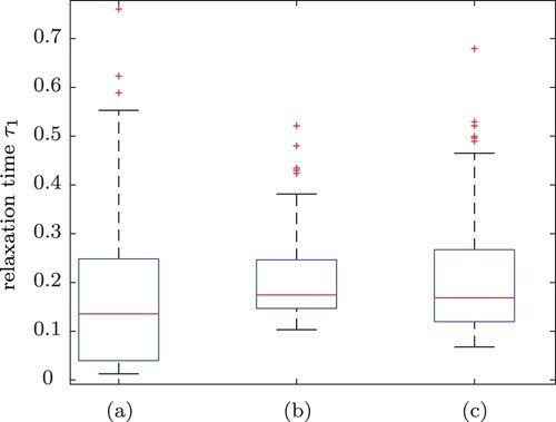
Figure 9. Largest relaxation time for 100 runs with (a) no regularization, (b) classical Tikhonov–Phillips regularization and (c) adjusted regularization term.

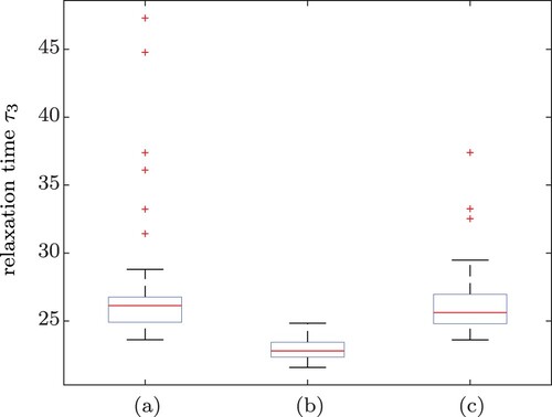
We see that we still manage to achieve a reasonable reconstruction of ${\tau }_1$ with the adjusted regularization term (see Figure 8 (c)). While ${\tau }_3$ was permanently reconstructed too small in the classical Tikhonov–Phillips regularization, we cannot observe such attenuation in (c), since we no longer penalize large values except ${\mu }_1$ (see Figure 9). In (15(15) $\Vert F(\mu ,{\mu }_1,\dots ,{\mu }_N,{\tau }_1,\dots {\tau }_N)-{\sigma }^{\delta }{\Vert }_2^2+\lambda {\mu }_1^2.$(15) ) we used $\lambda =0.135$ as regularization parameter, again determined by trial-and-error.

5.5. Shortened data sets

The last set of numerical experiments examines the effects of using a smaller number of data. This is interesting in view of shortening the duration of the experiment or sampling the data at a lower frequency. It is particularly relevant for the reconstruction of Maxwell elements with high relaxation times. Since we do not know these, we cannot estimate how long it takes for the stress contribution of this element to decay to zero. In other words: it is unclear at which time a material finds its equilibrium or reaches a point where the difference between the current stress and the asymptotic stress is less than the experimental noise. This is why in the following we will test reconstructions from shortened data sets in order to be able to make an assertion about the accuracy of these reconstructions.

We again work with noisy data (${\delta }_{rel}\approx 1\mathrm{\%}$), N = 5, for the minimization and use the adapted penalty term (15(15) $\Vert F(\mu ,{\mu }_1,\dots ,{\mu }_N,{\tau }_1,\dots {\tau }_N)-{\sigma }^{\delta }{\Vert }_2^2+\lambda {\mu }_1^2.$(15) ). Up to now, we have used a time interval of $[0,100]$ seconds with 1000 data points in our experiments, i.e. one data point any 0.1 seconds. We will now repeatedly shorten this data set by 5 s until we get a total time of 25 s. The results of the corresponding reconstructions are shown in Figure 10. We focus on the basic elasticity μ and stiffness ${\mu }_3$ of the Maxwell element with slowest relaxation time and furthermore on the smallest and largest relaxation times ${\tau }_1$ and ${\tau }_3$. The behaviour of the central Maxwell element is comparable to the third one, which is why we omit a detailed discussion.

Figure 10. Effect of reducing the duration $[0,T]$ of the experiment on the material parameters $\mu ,{\mu }_3,{\tau }_1$ and ${\tau }_3$ for a displacement rate of 10 mm/s (left) and 1 mm/s (right), respectively.

The basic elasticity μ of the single spring can perfectly be identified after only 25 s for a displacement rate of 10 mm/s. For the slower rate of 1 mm/s, 55 s of the experiment are necessary for a reliable identification. The minimal time to conclusively identify the stiffness ${\mu }_3$ of the spring in the third Maxwell element takes 40 s for a rate of 10 mm/s and 50 s for a rate of 1 mm/s, respectively.

The identification of the relaxation times is more difficult than of the stiffnesses. The relaxation times ${\tau }_3$ of the third Maxwell element can be precisely determined after 45 s for a rate of 10 mm/s and after 70 s for the slower rate of 1 mm/s, respectively. After that the result gets worse with every second the data set is shortened. There are not sufficient data points left to perform a reliable reconstruction. The variation in the values for the fastest relaxation time ${\tau }_1$ is much larger than for ${\tau }_3$ and also very sensitive to noise. Experimental observations show in general that, if the displacement rate is too high, the third Maxwell element with the slowest relaxation time behaves like an equilibrium spring since there is not enough time to relax during loading. The stiffness of the third element superimposes with the equilibrium spring. However, during relaxation the equilibrium spring and the third Maxwell element can be easily distinguished from each other. Hence, the faster loading rate of 10 mm/s can predict μ and ${\mu }_3$ even with 30 s of the data whereas, for the 1 mm/s loading rate, at least 50 s of data is required for accurate prediction. On the other hand the prediction of ${\tau }_1$ is easier with the 10 mm/s data because, if the displacement rate is too low, the first Maxwell element with the fastest relaxation time starts to relax during the loading itself. This is shown for a rate of 1 mm/s in Figure 10. A satisfying identification is not possible during the entire experimental duration of 100 s. However, for the faster rate of 10 mm/s ${\tau }_1$ it can already be determined after 50 s. We like to mention that the curves in Figure 10 look much more similar if we only consider the phase where the strain is held constant, i.e. by neglecting the first 20  s.

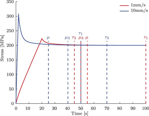
As a summary of the observations above and for a better understanding, Figure 11 again shows the stress–time curves for the two different displacement rates, but now including the time in the experiments to identify the individual material parameters. The parameters are not of the same order for the different rates. For instance, for a displacement rate of 1mm/s the relaxation time ${\tau }_3$ can be reconstructed first, while at 10mm/s the stiffness μ is most stable to data shortening. Thus, no general statement can be made about a correlation of the material parameters and the duration of the experiment without considering conditions such as the displacement rate.

Figure 11. Synthetic stress–time data produced by a spring combined with a three Maxwell element model including the duration of the experiment to conclusively identify the stiffnesses and relaxation times for displacement rates of 1 mm/s and 10 mm/s.

6. Conclusion and future work

In this paper, we presented an algorithm for the reconstruction of material parameters in a Maxwell-based rheological multi-parameter model for viscoelastic materials under stress–time conditions that are realistic for tensile tests in a laboratory. After a short introduction to the material model, we defined the forward operator and proposed an analytical way to solve the evolution equation with respect to relaxation times. This allowed us to determine an analytical solution of the forward operator with regard to the number of Maxwell elements given specific stress–time curves.

A big challenge and novelty compared to classical settings in inverse problems is represented by the fact that the forward operator F depends on the number of Maxwell elements n and, thus, on parts of the searched solution itself. This uncertainty is overcome by using an appropriate clustering algorithm, which is new in this field. For the parameter identification, we considered different approaches based on minimizing a least squares functional. In experiments we have seen that the simple approach to minimize the residual is not sufficient for perturbed data and especially the material parameters of the Maxwell element with shortest relaxation time is very susceptible to noise. By analysing the stress–time curve decomposed into the single spring and Maxwell element stresses, we were able to give a clear recommendation towards higher displacement rates. This analysis also contributed to the understanding of why the small relaxation times with their corresponding stiffness are that sensitive to noise. This proves the great relevance of our theoretical and numerical investigations for the performance of future experiments such as tensile tests.

Subsequently, we considered various regularization methods such as the classical Tikhonov–Phillips approach. We conclude that a specific regularization adapted to the smallest relaxation time is preferable. This confirms former investigations regarding the condition of the underlying problem in [23].

Investigations on shortened data sets demonstrate that our approach for material parameter identification shows great advantages for performing real experiments since it yields suggestions on the minimum duration of the experiments. This is very important because typical relaxation experiments can last days or weeks until the basic elasticity can be determined using conventional evaluation methods. In that sense our new approach might be of significant interest for the identification of parameters in materials science.

Nearly all polymers show more or less a viscoelastic behaviour. Hence, the stress relaxation problem is a real problem and of utmost importance. Although the generalized Maxwell model is well known in theory, from the experimental point of view it is not possible to simply fit the data by a decaying exponential function since it never reaches the basic elasticity needed to simulate the materials. Basic elasticity would only be reached at infinite time leading to an infinite duration of the experiments. Therefore, the new approach is of great importance for the reliable experimental determination of the material parameters of viscoelastic materials and therefore also for the simulation of such materials.

Future research is focused on validating the presented algorithms on real data sets. However, at this point, real scattering date are not suitable, since we do not know the real parameters. Therefore, we did first a parameter re-identification in this work to check the performance of our new approach. Furthermore, it might be interesting to apply other numerical regularization methods, such as the Landweber iteration or Newton type methods combined with Bayes inversion.

Disclosure statement

No potential conflict of interest was reported by the author(s).

References

- Hartmann S, Neff P. Polyconvexity of generalized polynomial-type hyperelastic strain energy functions for near-incompressibility. Int J Solids Struct. 2003;40(11):2767–2791.
- Woestehoff A, Schuster T. Uniqueness and stability result for Cauchy's equation of motion for a certain class of hyperelastic materials. Appl Anal. 2015;94(8):1561–1593.
- Binder F, Schöpfer F, Schuster T. Defect localization in fibre-reinforced composites by computing external volume forces from surface sensor measurements. Inverse Probl. 2015;31(2):025006.
- Seydel J, Schuster T. On the linearization of identifying the stored energy function of a hyperelastic material from full knowledge of the displacement field. Math Methods Appl Sci. 2017;40(1):183–204.
- Seydel J, Schuster T. Identifying the stored energy of a hyperelastic structure by using an attenuated Landweber method. Inverse Probl. 2017;33(12):124004.
- Klein R, Schuster T, Wald A. Sequential subspace optimization for recovering stored energy functions in hyperelastic materials from time-dependent data. In: Kaltenbacher B, Schuster T, Wald A, editors. Time-dependent problems in imaging and parameter identification. Berlin: Springer; 2021. p. 165–190.
- Rothermel D, Schuster T. Solving an inverse heat convection problem with an implicit forward operator by using a projected Quasi-Newton method. Inverse Problems. 2021.37:045014
- Rothermel D, Schuster T, Schorr R et al.. Parameter estimation of temperature dependent material parameters in the cooling process of TMCP steel plates. Mathematical Problems in Engineering. 2021.https://doi.org/10.1155/2021/6653388.
- Colton DL, Kress R. Inverse acoustic and electromagnetic scattering theory. Berlin: Springer; 1998.
- Wald A, Schuster T. Terahertz tomographic imaging using sequential subspace optimization. In: Hofmann B, Leitao A, Zubelli JP, editors. New trends in parameter identification for mathematical models. Basel: Birkhäuser; 2018. (Trends in Mathematics).
- Chen Z, Scheffer T, Seibert H, et al. Macroindentation of a soft polymer: identification of hyperelasticity and validation by uni/biaxial tensile tests. Mech Mater. Sep 2013;64:117–127.
- Heinze S, Bleistein T, Düster A, et al. Experimental and numerical investigation of single pores for identification of effective metal foams properties. ZAMM – J Appl Math Mechs / Z Ange Math Mech. 2018;98(5):682–695.
- Gavrus A, Massoni E, Chenot JL. An inverse analysis using a finite element model for identification of rheological parameters. J Mater Processing Technol. 1996;60(1–4):447–454.
- Hartmann S. Parameter estimation of hyperelasticity relations of generalized polynomial-type with constraint conditions. Int J Solids Struct. 2001;38(44–45):7999–8018.
- Hartmann S. Numerical studies on the identification of the material parameters of Rivlin's hyperelasticity using tension-torsion tests. Acta Mech. 2001;148(1):129–155.
- Mahnken R, Stein E. A unified approach for parameter identification of inelastic material models in the frame of the finite element method. Comput Methods Appl Mech Eng. 1996;136(3–4):225–258.
- Scheffer T, Seibert H, Diebels S. Optimisation of a pretreatment method to reach the basic elasticity of filled rubber materials. Arch Appl Mech. Nov 2013;83(11):1659–1678.
- Bonfanti A, Kaplan JL, Charras G, et al. Fractional viscoelastic models for power-law materials. Soft Matter. 2020;16(26):6002–6020.
- Jalocha D. Payne effect: a constitutive model based on a dynamic strain amplitude dependent spectrum of relaxation time. Mech Mater. 2020;148:103526.
- Sharma P, Sambale A, Stommel M, et al. Moisture transport in PA6 and its influence on the mechanical properties. Continuum Mech Thermodyn. 2020;32(2):307–325.
- Tschoegl NW. The phenomenological theory of linear viscoelastic behavior. Heidelberg: Springer; 1989.
- Wineman AS, Rajagopal KR. Mechanical response of polymers: an introduction. Cambridge, UK: Cambridge University Press; 2000.
- Diebels S, Scheffer T, Schuster T, et al. Identifying elastic and viscoelastic material parameters by means of a Tikhonov regularization. Math Probl Eng. Feb 2018;2018:1–11.
- Fernanda M, Costa P, Ribeiro C. Parameter estimation of viscoelastic materials: a test case with different optimization strategies. International Conference on Numerical Analysis and Applied Mathematics (ICNAAM), AIP Conf. Proc.; Vol. 1389, 2011. p. 771–774.
- Shukla K, Chan J, de Hoop MV. A high order discontinuous Galerkin method for the symmetric form of the anisotropic viscoelastic wave equation. 2020. Available from: arXiv:2011.01529v1.
- Park SW, Schapery R. Methods of interconversion between linear viscoelastic material functions. part I – a numerical method based on Prony series. Int J Solids Struct. 1999;36:1653–1675.
- Emri I, Tschoegl NW. An iterative computer algorithm for generating line spectra from linear viscoelastic response functions. Int J Polymeric Mater Polymeric Biomater. 1998;40:55–79.
- Engl HW, Hanke M, Neubauer A. Regularization of inverse problems. Vol. 375. Netherlands: Springer Science & Business Media; 2000.
- Louis AK. Inverse und schlecht gestellte probleme. Berlin: Springer-Verlag; 2013.
- Rieder A. Keine Probleme mit inversen Problemen: eine Einführung in ihre stabile Lösung. Berlin: Springer-Verlag; 2013.
- Kirsch A. An introduction to the mathematical theory of inverse problems. Berlin: Springer; 2011.
- Kaltenbacher B, Neubauer A, Scherzer O. Iterative regularization methods for nonlinear ill-posed problems. Vol. 6. Germany: Walter de Gruyter; 2008.
- Wald A, Schuster T. Sequential subspace optimization for nonlinear inverse problems. J Inv Ill-posed Problems. 2017;25(1):99–117.
- Wald A. A fast subspace optimization method for nonlinear inverse problems in Banach spaces with an application in parameter identification. Inverse Probl. 2018;34(8):085008.
- Provencher SW. CONTIN: a general purpose constrained regularization program for inverting noisy linear algebraic and integral equations. Comput Phys Commun. 1982;27:229–242.
- Goldschmidt F, Diebels S. Modelling and numerical investigations of the mechanical behavior of polyurethane under the influence of moisture. Arch Appl Mech. 2015;85(8):1035–1042.
- Johlitz M, Steeb H, Diebels S, et al. Experimental and theoretical investigation of nonlinear viscoelastic polyurethane systems. J Mater Sci. 2007. 42(23)9894–9904.
- Baurngaertel M, De Rosa ME, Machado J, et al. The relaxation time spectrum of nearly monodisperse polybutadiene melts. Rheol Acta. 1992;31(1):75–82.
- Berry GC, Fox TG. The viscosity of polymers and their concentrated solutions. Fortschritte der Hochpolymeren-Forschung. Berlin: Springer; 1968. p. 261–357.
- Johlitz M, Lion A. Chemo-thermomechanical ageing of elastomers based on multiphase continuum mechanics. Continuum Mech Thermodyn. 2013;25(5):605–624.
- Reese S, Govindjee S. A theory of finite viscoelasticity and numerical aspects. Int J Solids Struct. 1998;35(26–27):3455–3482.
- Croft LR, Goodwill PW, Conolly SM. Relaxation in x-space magnetic particle imaging. IEEE Trans Med Imaging. 2012;31(12):2335–2342.
- Colton D, Kress R. Inverse acoustic and electromagnetic scattering theory. Berlin: Springer; 1992.
- Goldschmidt F, Diebels S. Modeling the moisture and temperature dependent material behavior of adhesive bonds. PAMM. 2015;15(1):295–296.
- Inc MathWorks. MATLAB: the language of technical computing. Desktop tools and development environment. version 7. Vol. 9, MathWorks; 2005.
- Engl HW, Kunisch K, Neubauer A. Convergence rates for Tikhonov regularisation of non-linear ill-posed problems. Inverse Probl. 1989;5(4):523–540.
- Neubauer A. Tikhonov regularization of nonlinear ill-posed problems in Hilbert scales. Appl Anal. 1992;46(1–2):59–72.
- Scherzer O. The use of Morozov's discrepancy principle for Tikhonov regularization for solving nonlinear ill-posed problems. Computing. 1993;51(1):45–60.