Inverse estimation of temperature-dependent refractive index profile in conductive-radiative media

Abstract

The aim of this paper is to retrieve the temperature-dependent refractive index distribution in parallel-plane semi-transparent media with combined conduction-radiation heat transfer, by the measurement of exit intensities over the boundaries. The finite volume method in combination with the discrete ordinates method is used to solve the energy equation. The results of the direct solution for both linear-spatially and linear-temperature-dependent refractive index distributions are compared and the effects of the main parameters are examined. The results confirm a remarkable difference between the results for spatially and temperature-dependent refractive index profiles. Finally, the refractive index profile is estimated using the conjugate gradient method in an inverse manner. The coefficients of the linear profile are estimated for three cases with different levels of measurement errors; 1%, 3% and 5%. The results show that the temperature-dependent refractive index distribution can be retrieved in a good range of errors for noisy data.

KEYWORDS:

• Inverse method
• conduction-radiation heat transfer
• refractive index
• semi-transparent media

2010 MATHEMATICS SUBJECT CLASSIFICATION:

• 80A23

Nomenclature

$d$	=	Direction of descent
$f$	=	Objective function
$G$	=	Incident radiation, $W/m^2$
$I$	=	Radiation intensity, $W/(m^2.sr)$
$J$	=	Sensitivity coefficient, $W/(m^2.sr)$
$K$	=	Thermal conductivity, $W/(m.K)$
$n$	=	Refractive index
$N_{cr}$	=	Conduction-radiation parameter
$q_r$	=	Radiative heat flux, $W/m^2$
$Q_r$	=	Non-dimensional radiative heat flux
$S$	=	Source term
$T$	=	Temperature, K
$Z$	=	Measured intensity, $W/(m^2.sr)$
$n_0$	=	Refractive index at the lower boundary
$n_L$	=	Refractive index at the upper boundary

Greek Symbols

$\alpha$	=	Search step size
$\beta$	=	Extinction coefficient, $1/m$
$\epsilon$	=	Emissivity
$\gamma$	=	Conjugation coefficient
${\kappa }_a$	=	Absorption coefficient, $1/m$
${\kappa }_s$	=	Scattering coefficient, $1/m$
$\mu$	=	Direction cosine
$\theta$	=	Non-dimensional temperature
$\sigma$	=	Steffan-Boltzmann constant, $W/(m^2.K^4)$
$\tau$	=	Optical thickness
$\omega$	=	Single scattering albedo

Subscripts

$w$	=	wall
$r$	=	radiative

Superscripts

$\upsilon$

=

Iteration number

1. Introduction

Due to the temperature-dependent variation of density in a radiating participating medium, the refractive index may be changed throughout the medium. As a result, the radiative rays may propagate along curve paths according to the Fermat principle [1].

In recent decades, more attempts have been made to solve the single-mode and multi-mode heat transfer with radiation in semi-transparent media (STM). Mishra et al. [2] used a combination of the lattice Boltzmann method (LBM) with the finite volume method (FVM) to solve the energy equation of a transient conduction-radiation heat transfer problem in a 1-D concentric cylindrical participating medium. When the spatial variation of the refractive index is continuous, the medium is called the graded index medium (GIM). The curved ray-tracing approaches have been widely used in the analysis of heat transfer in GIM [3–8]. However, because of the complexity of curved ray tracing, other methods have been developed to solve the radiative transfer equation (RTE) in GIM without curved ray tracing. Among them, the finite element method (FEM) [9–12], FVM [13–14], meshless approach [15,16], and spectral collocation method [17,18] are to be mentioned. More recently, Krishna and Mishra [19] and Hosseini Sarvari [20,21] solved the RTE in variable refractive index media by the discrete transfer method (DTM). The combination of the DTM with the lattice-Boltzmann method was used by Mishra et al. [22] to solve the combined conduction-radiation heat transfer with variable thermal conductivity and refractive index. The application of the discrete ordinates method (DOM) for solving the RTE in GIM with monotonic spatial variation of the refractive index has been developed by Lemonier and Le Dez [23] and has been extended to semi-transparent media with a non-continuous variation of refractive index by Hosseini Sarvari [24].

During the past few years, the inverse methods have been widely used for the estimation of the thermal properties in multimode heat transfer problems with radiation [25–37]. However, a few studies have been reported on inverse problems in the STM setting with the variable refractive index. The earliest work in this field was proposed by Liu [38], who used the backward Monte Carlo method in combination with the conjugate gradient method (CGM) to reconstruct the source term in a plane-parallel absorbing-emitting GIM. Namjoo et al. [39] used an inverse approach for reconstruction of temperature distribution in an absorbing, emitting, and anisotropically scattering GIM by the measurement of exit intensities. They used the DOM for solving the RTE, and the CGM to minimize the objective function. Khayyam and Hosseini Sarvari [40] used the inverse approach to estimate the thermal properties in a plane-parallel GIM. Namjoo et al. [41] adopted the CGM for simultaneous estimation of source term and boundary refractive indices in a GIM with linear refractive index profile. Estimation of arbitrary refractive index distribution in GIM was reported by Namjoo et al. [42]. Wei et al. [43,44] used the particle swarm optimization (PSO) algorithm to retrieve the conduction-radiation parameter and refractive index profile by the measurement of optical and thermal information.

In all the above-mentioned inverse problems, the variation of the refractive index has been assumed to be constant or spatially dependent. However, due to the change of density with temperature in a participating medium, the refractive index is a function of temperature. In all the previous works in the field of inverse heat transfer, the refractive index has been considered to be constant, or a function of spatial coordinates. The main goal of the present paper is to examine the effects of temperature-dependent refractive index on the solution of inverse problem and comparing its results with those obtained by spatially dependent refractive index. To the knowledge of the authors, no inverse analysis has been reported to retrieve the temperature-dependent refractive index profile in the GIM. In this paper, we compare the temperature distribution within the media for both spatially and temperature-dependent refractive index and show the importance of this assumption, and then we try to retrieve the temperature-dependent refractive index profile in a conductive-radiative plane-parallel GIM by the measurement of exit intensities over the boundaries. The energy equation for combined conduction-radiation heat transfer is solved by the combination of the FVM-DOM. The CGM is used to minimize the objective function to retrieve the temperature-dependent refractive indices over the boundaries. The direct solution is verified by comparing the results with a benchmark solution. The effects of the conduction-radiation parameter, optical thickness, and single scattering albedo are investigated by some numerical examples. The influence of measurement errors is also examined by imposing artificial errors in measured data. The results show that the temperature-dependent refractive index profile can be well recovered, even for high noisy data.

2. Description of problem

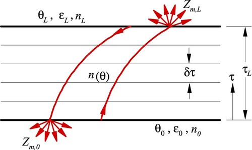
Consider a one-dimensional medium between two parallel plates at constant temperatures, as illustrated in Figure 1. The medium is semitransparent with emitting, absorbing, and isotropic scattering. Both plates are diffuse-gray with constant emissivities. In this study, we consider the combined conduction-radiation heat transfer mechanism, and the effects of convection heat transfer are neglected. All the medium's properties are assumed to be constant whereas the refractive index varied with the temperature of the medium. The aim of the inverse problem is to retrieve the temperature-dependent refractive index distribution by the measurement of wall radiative intensities.

Figure 1. Schematic of plane-parallel GIM with diffuse-gray walls.

3. The direct problem

In the absence of heat generation and convection, the non-dimensional form of the energy equation for 1-D steady-state combined conduction-radiation heat transfer in a participating medium can be written as [45]: (1a) $\begin{array}{rl}\frac{d^2\theta }{d{\tau }^2}& =\frac{1}{N_{cr}}\frac{d{Q}_r}{d\tau },0\le \tau \le {\tau }_L\end{array}$(1a) (1b) $\begin{array}{rl}\theta (0)& =1\end{array}$(1b) (1c) $\begin{array}{rl}\theta ({\tau }_L)& ={\theta }_L\end{array}$(1c) where $\theta =T/T_0$ is the non-dimensional temperature. In Equation (1a), $\tau$ is the optical thickness, $N_{cr}=K\beta /(4\sigma T_0^3)$ is the conduction-radiation parameter, and $Q_r=q_r/(4\sigma T_0^4)$ is the non-dimensional radiative heat flux.

The conservative form of the RTE and its associated boundary conditions in a semitransparent GIM is [23]: (2a) $\begin{array}{rl}& \mu {\frac{\mathrm{\partial }I}{\mathrm{\partial }\tau }|}_{\mu }+\gamma (\theta ,\tau ){\frac{\mathrm{\partial }([1-{\mu }^2]I)}{\mathrm{\partial }\mu }|}_{\tau }+\beta I=S\end{array}$(2a) (2b) $\begin{array}{rl}& I(0)={\epsilon }_0{n}_0^2{I}_{b,0}+2(1-{\epsilon }_0){\int }_{-1}^{0}I(0,\mu )\mu d\mu \end{array}$(2b) (2c) $\begin{array}{rl}& I({\tau }_L)={\epsilon }_L{n}_L^2{I}_{b,L}+2(1-{\epsilon }_L){\int }_0^{+1}I({\tau }_L,\mu )\mu d\mu \end{array}$(2c) where $\beta ={\kappa }_a+{\kappa }_s$ and (3) $S=(1-\omega )n^2(\theta )I_b+\frac{\omega }{4\pi }G(\tau )$(3) where $I(\tau ,\mu )$ is the radiation intensity in the direction whose cosine along the $\tau \text{ - }axis$ is μ, and $\omega ={\kappa }_s/\beta$ is the single scattering albedo. $\gamma (\theta ,\tau )$ is defined as (4) $\gamma (\theta ,\tau )=\frac{1}{2n^2(\theta )}\frac{d{n}^2(\theta )}{d\theta }\frac{d\theta }{d\tau }$(4)

The equations for incident radiation and radiative heat flux are given by (5a) $\begin{array}{rl}G(\tau )& =2\pi {\int }_{-1}^{+1}I(\tau ,\mu )d\mu \end{array}$(5a) (5b) $\begin{array}{rl}{q}_r(\tau )& =2\pi {\int }_{-1}^{+1}I(\tau ,\mu )\mu d\mu \end{array}$(5b)

The non-dimensional divergence of radiative heat flux, $d{Q}_r/d\tau$, is obtained by the following equation: (6) $\frac{d{Q}_r}{d\tau }=(1-\omega )[n^2{\theta }^4-G/(4\sigma T_0^4)]$(6)

The refractive index distribution is dependent on temperature by a linear profile as (7) $n(\theta )=(n_L-n_0)(\theta -1)/({\theta }_L-1)+n_0$(7)

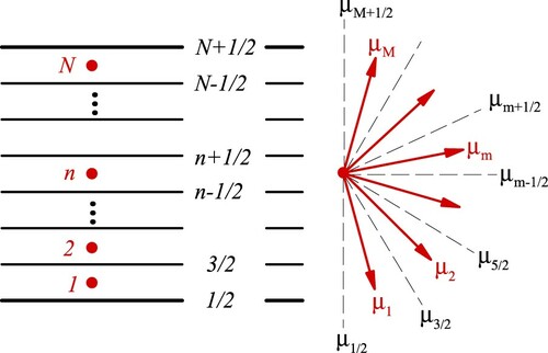
In this study, we use the DOM for solving the RTE and FVM for solving the energy equation. In the DOM, the solution domain is divided into N slices control volumes of width ${\delta }_{\tau }$ and the angular domain is divided into M discrete ordinates with equally spaced distribution of $\mu$ and a constant weight quadrature, $w_m=2/M$, where $w_m$ is the weight associated to ${\mu }_m$. The division of spatial and angular domain is illustrated in Figure 2. Integration of the RTE over the control volume and over the solid angle leads to (8) $\begin{array}{rl}& {\mu }_m{w}_m(I_{m,n+1/2}-I_{m,n-1/2})+{\gamma }_n{\delta }_{\tau }({\alpha }_{m+1/2}{I}_{m+1/2,n}-{\alpha }_{m-1/2}{I}_{m-1/2,n})+\beta w_m{\delta }_{\tau }{I}_{m,n}\\ & =S_{m,n}{w}_m{\delta }_{\tau }\end{array}$(8) where ${\alpha }_{m\pm 1/2}=1-{\mu }_{m\pm 1/2}^2$. For temperature-dependent refractive index, we have: (9) ${\gamma }_n{\delta }_{\tau }=\frac{1}{n(\theta )}\frac{n_L-n_0}{{\theta }_L-1}({\theta }_{n+1}-{\theta }_{n-1})$(9)

Figure 2. Spatial and angular division of the domain.

In each control volume, there are three unknown intensities in Equation (8). Hence, for their calculation, we need two supplementary equations. These equations are determined by the interpolation over each volume as follows (10a) $\begin{array}{rl}{I}_{m,e}& \simeq \frac{1}{a_{\tau }}\frac{n_e^2}{n_n^2}{I}_{m,n}+\left(1-\frac{1}{a_{\tau }}\right)\frac{n_e^2}{n_w^2}{I}_{m,w}\end{array}$(10a) (10b) $\begin{array}{rl}{I}_{t,n}& \simeq \frac{I_{m,n}}{a_{\mu }}+\left(1-\frac{1}{a_{\mu }}\right)I_{c,n}\end{array}$(10b) with $1/2\le a_{\tau },a_{\mu }\le 1$. Eventually, the incident intensity in each control volume is calculated by (11) $I_{m,n}=\frac{A_m[1-(1-1/a_{\tau })(n_e^2/n_w^2)]I_{m,w}+[B_{b,n}-B_{t,n}(1-1/a_{\tau })]I_{b,n}+D_{m,n}}{A_m{n}_w^2/a_{\tau }{n}_n^2+B_{t,n}/a_{\mu }+C_{m,n}}$(11) where $e=i+sign({\mu }_m)/2$, $w=i-sign({\mu }_m)/2$, $t=m+sign(n_i^{\mathrm{\prime }})/2$, and $b=m-sign(n_i^{\mathrm{\prime }})/2$, where $n_i^{\mathrm{\prime }}$ is the local derivative of n.

The parameters in Equation (11) are (12a) $\begin{array}{rl}{A}_m& =|{\mu }_m|w_m\end{array}$(12a) (12b) $\begin{array}{rl}{B}_{m\pm 1/2,n}& =\frac{n_L-n_0}{n_n}\frac{|{\theta }_{n+1/2}-{\theta }_{n-1/2}|}{{\theta }_L-1}{\alpha }_{m\pm 1/2}\end{array}$(12b) (12c) $\begin{array}{rl}{C}_{m,n}& ={\kappa }_{a,n}{w}_m{\delta }_{\tau }\end{array}$(12c) (12d) $\begin{array}{rl}{D}_{m,n}& =w_m{\delta }_{\tau }{S}_{m,n}\end{array}$(12d)

The boundary conditions are obtained from Equations (2a) and (2b) as (13a) $\begin{array}{rl}{I}_{m,0}& ={\epsilon }_0{n}_0^2{I}_{b,0}+2(1-{\epsilon }_0){\sum }_{m^{\mathrm{\prime }}=M/2+1}^M{w}_{m^{\mathrm{\prime }}}{\mu }_{m^{\mathrm{\prime }}}{I}_{m^{\mathrm{\prime }},0}d\mu \end{array}$(13a) (13b) $\begin{array}{rl}{I}_{m,L}& ={\epsilon }_L{n}_L^2{I}_{b,L}+2(1-{\epsilon }_L){\sum }_{m^{\mathrm{\prime }}=1}^{M/2}{w}_{m^{\mathrm{\prime }}}{\mu }_{m^{\mathrm{\prime }}}{I}_{m^{\mathrm{\prime }},L}d\mu \end{array}$(13b)

The incident radiation and radiative heat flux over the n-th control volume are approximated by (14a) $\begin{array}{rl}{G}_n& =2\pi {\sum }_{m=1}^M{w}_m{I}_{m,n}\end{array}$(14a) (14b) $\begin{array}{rl}{q}_n& =2\pi {\sum }_{m=1}^M{w}_m{\mu }_m{I}_{m,n}\end{array}$(14b)

The application of the DOM is limited to a medium with a monotonic refractive index profile, where the gradient of the refractive index has a uniform sign over the medium [23].

The energy equation is solved by the FVM [46]. As seen in Equation (1a), the contribution of the radiation heat transfer is imposed to the energy equation as a thermal heat source. This source term is (15) ${\frac{d{Q}_r}{d\tau }|}_n=(1-{\omega }_n)[n_n^2{\theta }_n^4-G_n/(4\sigma T_0^4)]$(15)

In Equation (15), ${\theta }^4$ causes the equation to be nonlinear, and must be linearized as (16) ${\theta }_{n,new}^4=4{\theta }_{n,old}^3{\theta }_n-3{\theta }_{n,old}^4$(16) where the subscripts new and old denote the values in current and previous iterations, respectively.

In each iteration, the incident radiation, G, is calculated by solving the RTE. Then the energy equation is solved by the FVM to obtain the temperature distribution. The iterative procedure is terminated when the absolute differences between all the temperatures for two successive iterations become less than a small value, say ${10}^{-6}$. The boundary heat fluxes are determined by the superposition of the conductive and radiative heat fluxes.

4. The inverse problem

The inverse problem is formulated as a minimization problem of an objective function defined by the following equation (17) $\begin{array}{rl}{f}^{\upsilon }(n_0,n_L)& ={\sum }_{m=1}^{M/2}{[Z_{m,0}({\mu }_m,n_0,n_L)-I_{m,0}^{\upsilon }({\mu }_m,n_0,n_L)]}^2\\ & +{\sum }_{m=M/2+1}^M{[Z_{m,L}({\mu }_m,n_0,n_L)-I_{m,L}^{\upsilon }({\mu }_m,n_0,n_L)]}^2\end{array}$(17) where $Z_{m,0}$ and $Z_{m,L}$ are the measured directional intensities over the boundaries. In order to minimize the objective function, the gradient of the objective function with respect to unknown parameters must be set to zero, (18) $\begin{array}{l}\mathrm{\nabla }{f}_k^{\upsilon }=\mathrm{\partial }{f}^{\upsilon }/\mathrm{\partial }{n}_k=2{\sum }_{m=1}^{M/2}{J}_{m,0}^{\upsilon }[I_{m,0}^{\upsilon }({\mu }_m,n_0,n_L)-Z_{m,0}({\mu }_m,n_0,n_L)]\\ +2{\sum }_{m=M/2+1}^M{J}_{m,L}^{\upsilon }[I_{m,L}^{\upsilon }({\mu }_m,n_0,n_L)-Z_{m,L}({\mu }_m,n_0,n_L)]=0\end{array}$(18) where the sensitivity coefficients, $J_{m,k}^{\upsilon }$, are defined as (19) $J_{m,k}^{\upsilon }=\frac{\mathrm{\partial }{I}_{m,k}^{\upsilon }}{\mathrm{\partial }{n}_k},k=0,L$(19)

The inverse approach is based on the CGM presented by Ozisik and Orlande [47]. For estimation of unknown parameters, first, an initial guess is made for $n_0^0$ and $n_L^0$. Then, the iterative procedure of the CGM is applied for taking a suitable step size along a direction of descent to update the unknown parameters as follows (20) $n_k^{\upsilon +1}=n_k^{\upsilon }+{\alpha }^{\upsilon }{d}_k^{\upsilon },k=0,L$(20) where ${\alpha }^{\upsilon }$ is search step size, and $d_k^{\upsilon }$ is the direction of descent associated to $n_k^{\upsilon }$. The direction of descent is calculated by (21) $d_k^{\upsilon }=\mathrm{\nabla }{f}_k^{\upsilon }+{\lambda }^{\upsilon }{d}_k^{\upsilon -1},k=0,L$(21) where the conjugation coefficient, $\lambda$, is calculated by the Fletcher-Reeves formula [47] (22) ${\lambda }^{\upsilon }={\sum }_k^{}{(\mathrm{\nabla }{f}_k^{\upsilon })}^2/{\sum }_k^{}{(\mathrm{\nabla }{f}_k^{\upsilon -1})}^{2}with{\lambda }^0=0,k=0,L$(22)

The search step size ${\alpha }^{\upsilon }$ appearing in Equation (20) is given by (23) ${\alpha }^{\upsilon }=\frac{{\sum }_{m=1}^{M/2}(J_{m,0}^{\upsilon }{d}_L^{\upsilon })(Z_{m,0}-I_{m,0}^{\upsilon })+{\sum }_{m=M/2+1}^M(J_{m,L}^{\upsilon }{d}_L^{\upsilon })(Z_{m,L}-I_{m,L}^{\upsilon })}{{\sum }_{m=1}^{M/2}(J_{m,0}^{\upsilon }{d}_0^{\upsilon })(J_{m,0}^{\upsilon }{d}_0^{\upsilon })+{\sum }_{m=M/2+1}^M(J_{m,L}^{\upsilon }{d}_L^{\upsilon })(J_{m,L}^{\upsilon }{d}_L^{\upsilon })}$(23)

The stopping criterion for the iterative procedure is (24) $f^{\upsilon }(n_0,n_L)<\xi$(24) where $\xi$ is a small positive number, say 10⁻⁶.

5. The sensitivity problem

The precise calculation of sensitivity coefficients has an important role in the minimization procedure of the CGM. The sensitivity coefficients, $J_{m,k}^{\upsilon }$, indicate the sensitivity of the measured intensities on the boundary with respect to the variation of unknown parameters, $n_0^{\upsilon },n_L^{\upsilon }$. The sensitivity coefficients are determined by differentiation of governing equation and boundary conditions, Equations (1), with respect to unknown parameters (25a) $\begin{array}{rl}& \frac{d^2}{d{\tau }^2}\left(\frac{\mathrm{\partial }{\theta }^{\upsilon }}{\mathrm{\partial }{n}_k^{\upsilon }}\right)=\frac{1}{N_{cr}}\frac{d}{d\tau }\left(\frac{\mathrm{\partial }{Q}_r^{\upsilon }}{\mathrm{\partial }{n}_k^{\upsilon }}\right),k=0,L\end{array}$(25a) (25b) $\begin{array}{rl}& {\frac{\mathrm{\partial }{\theta }^{\upsilon }}{\mathrm{\partial }{n}_k^{\upsilon }}|}_{\tau =0}=0,k=0,L\end{array}$(25b) (25c) $\begin{array}{rl}& {\frac{\mathrm{\partial }{\theta }^{\upsilon }}{\mathrm{\partial }{n}_k^{\upsilon }}|}_{\tau ={\tau }_L}=0,k=0,L\end{array}$(25c)

and differentiation of the RTE with associated boundary conditions, Equation (2), with respect to unknown parameters leads to (26a) $\begin{array}{rl}& \mu {\frac{\mathrm{\partial }}{\mathrm{\partial }\tau }\left(\frac{\mathrm{\partial }{I}^{\upsilon }}{\mathrm{\partial }{n}_k^{\upsilon }}\right)|}_{\mu }+\frac{\mathrm{\partial }\gamma }{\mathrm{\partial }{n}_k^{\upsilon }}{\frac{\mathrm{\partial }([1-{\mu }^2]I^{\upsilon })}{\mathrm{\partial }\mu }|}_{\tau }+\gamma {\frac{\mathrm{\partial }}{\mathrm{\partial }\mu }\left([1-{\mu }^2]\frac{\mathrm{\partial }{I}^{\upsilon }}{\mathrm{\partial }{n}_k^{\upsilon }}\right)|}_{\tau }+\beta \frac{\mathrm{\partial }{I}^{\upsilon }}{\mathrm{\partial }{n}_k^{\upsilon }}=\frac{\mathrm{\partial }{S}^{\upsilon }}{\mathrm{\partial }{n}_k^{\upsilon }}\\ & k=0,L\end{array}$(26a) (26b) $\begin{array}{rl}& {\frac{\mathrm{\partial }{I}^{\upsilon }}{\mathrm{\partial }{n}_k^{\upsilon }}|}_{\tau =0}=2{\epsilon }_0{n}_0^{\upsilon }{I}_{b,0}\frac{\mathrm{\partial }{n}_0^{\upsilon }}{\mathrm{\partial }{n}_k^{\upsilon }}+2(1-{\epsilon }_0){\int }_{-1}^0\frac{\mathrm{\partial }{I}^{\upsilon }(0,\mu )}{\mathrm{\partial }{n}_k^{\upsilon }}\mu d\mu \\ & k=0,L\end{array}$(26b) (26c) $\begin{array}{rl}& {\frac{\mathrm{\partial }{I}^{\upsilon }}{\mathrm{\partial }{n}_k^{\upsilon }}|}_{\tau ={\tau }_L}=2{\epsilon }_L{n}_L^{\upsilon }{I}_{b,L}\frac{\mathrm{\partial }{n}_L^{\upsilon }}{\mathrm{\partial }{n}_k^{\upsilon }}+2(1-{\epsilon }_L){\int }_0^1\frac{\mathrm{\partial }{I}^{\upsilon }(L,\mu )}{\mathrm{\partial }{n}_k^{\upsilon }}\mu d\mu ,k=0,L\end{array}$(26c) where (27) $\begin{array}{rl}\frac{\mathrm{\partial }{S}^{\upsilon }}{\mathrm{\partial }{n}_k^{\upsilon }}& =2(1-\omega )n^{\upsilon }\frac{\mathrm{\partial }{n}^{\upsilon }}{\mathrm{\partial }{n}_k^{\upsilon }}{I}_b^{\upsilon }+(1-\omega )(n^{\upsilon }{)}^2\frac{\mathrm{\partial }{I}_b^{\upsilon }}{\mathrm{\partial }{n}_k^{\upsilon }}+\frac{\omega }{2}{\int }_{-1}^{+1}\frac{\mathrm{\partial }{I}^{\upsilon }(\tau ,{\mu }^{\mathrm{\prime }})}{\mathrm{\partial }{n}_k^{\upsilon }}\mathrm{\Phi }(\mu ,{\mu }^{\mathrm{\prime }})d{\mu }^{\mathrm{\prime }}\\ & k=0,L\end{array}$(27)

The solution procedure of the sensitivity problem is similar to the solution procedure of the direct problem. However, some additional source terms appeared in Equations (26) and (27) are recalled from the solution of the direct problem.

6. Simulation of measured data

In order to simulate the measured exit intensities, the exact exit intensities calculated from the solution of the direct problem are added to the random errors of normally distribution, $\rho$, multiplied by the standard deviation, as follows [47]: (28) $Z_{m,k}=I_{m,k}^{exact}+\rho {\chi }_{m,k},k=0,L$(28) where $\rho$ is a normal distributed random error with zero mean and unit standard deviation, and the standard deviation, ${\chi }_m$, is determined by (29) ${\chi }_{m,k}=I_{m,k}^{exact}\times \eta /2.576,k=0,L$(29) where $\eta$ is the measurement error associated with the measured data.

In this study, 40 exit intensities are measured on each boundary, so that $M=40$_.

7. The computational algorithm

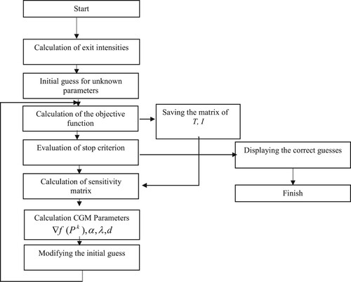
The computational procedure for inverse CGM is summarized as follows

1. Step 1 – Set v = 0 and guess the initial values for $n_k^v,k=0,L$.

2. Step 2 – Solve the direct problem, Equation (6), compute the temperature field in the medium and exit intensities over the lower and upper boundaries.

3. Step 3 – Calculate the objective function, Equation (17).

4. Step 4 – Solve the sensitivity problem and obtain the sensitivity coefficients.

5. Step 5 – Terminate the iterative procedure if the stopping criterion is satisfied. Otherwise, go to the next step.

6. Step 6 – Compute the gradient direction $\mathrm{\nabla }{f}_k^{\upsilon }$ by Equation (18) and the conjugation coefficient ${\lambda }^{\upsilon }$ by Equation (22).

7. Step 7 – Calculate the direction of descent $d_k^{\upsilon }$ by Equation (21).

8. Step 8 – Compute the search step size ${\alpha }^v$ by Equation (23).

9. Step 9 – Calculate the new unknown parameters by Equation (20).

10. Step 10 – Replace v by v+1 and return to Step 2.

The algorithm of the inverse procedure is depicted in Figure 3.

Figure 3. Inverse method algorithm.

8. Results and discussion

8.1. Verification of the solution of the direct problem

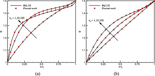
In order to verify the performance and accuracy of the direct problem, we compare the temperature distributions obtained from the present method by those obtained by Ben-Abdallah and Le Dez [3] for a 1-D conductive-radiative parallel-plane GIM with black walls and linear spatially dependent refractive index distribution with $n_0=1.2,n_L=1.8$. The comparisons are shown in Figure 4(a,b). As seen, the results are in good agreement.

Figure 4. Temperature distribution along with a 1 cm-depth slab for different values of the absorption coefficient with ${\theta }_0=1$ and ${\theta }_L=1.5$ (a) $K=0.1W/mK$, (b) $K=1.0W/mK$_.

8.2. The results of the direct problem

In this section, the effect of the temperature-dependent refractive index is investigated. We compare the results for two media with temperature-dependent and spatially dependent refractive index profiles. Consider a 1-D slab with wall temperatures of ${\theta }_0=1,{\theta }_L=1.5$. In order to compare the results of temperature-dependent and spatially dependent refractive index distributions, the refractive indices over the boundaries for both cases must be the same. Therefore, we consider two distinct functions for the refractive index as follows: (30a) $\begin{array}{rl}{n}_{\tau }(\tau )& =(n_L-n_0)\tau /{\tau }_L+n_0\end{array}$(30a) (30b) $\begin{array}{rl}n(\theta )& =(n_L-n_0)(\theta -1)/({\theta }_L-1)+n_0\end{array}$(30b)

The temperature profiles for both cases are compared in Figure 5(a,b) for different values of $N_{cr}$. As seen in Figure 4(a), for the low-gradient case, $n_0=1.2,n_L=1.8$, the difference between the results for both cases is more evident for low values of $N_{cr}$, where the problem tends to pure radiation. However, for the high-gradient case, $n_0=1,n_L=3$, by increasing the refractive index gradient, the deviation between the results is increased, even for large values of $N_{cr}$ (see Figure 5(b)).

Figure 5. Temperature distribution along a parallel-plane GIM with temperature-dependent and location-dependent refractive index profiles for different values of the conduction-radiation parameter, (a) $n_0=1.2,n_L=1.8$, (b) $n_0=1,n_L=3$.

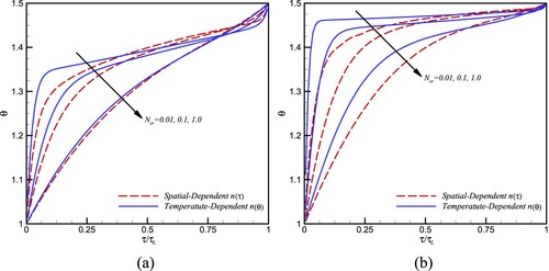
The above-mentioned discussions show that ignoring temperature-dependent effects cause a significant error in the analysis of conduction-radiation heat transfer in GIM.

8.3. The results of the inverse problem

In this part, we try to estimate three different linear temperature-dependent refractive index profiles with various gradients. The non-dimensional temperatures over the walls are ${\theta }_0=1,{\theta }_L=1.5$, and the emissivities are ${\epsilon }_0=0.7,{\epsilon }_L=0.5$.

Here, we try to estimate the unknown parameters, $n_0$ and $n_L$, for three different values of measurement errors, $\eta$. For the first case, we examine the effect of $N_{cr}$ and the gradient of refractive index profile on the estimated values. Hence, we use the inverse approach with three conduction-radiation parameters and three refractive index profiles. The results are shown in Table 1. As seen, the CGM has a good performance for estimation the unknown parameters for different values of the conduction-radiation parameter, even with highly noisy data. The rate of convergence for objective function with $N_{cr}=0.01$, $\eta =0.05$, and different values of refractive ratio $n_L/n_0$ is shown in Figure 6. As seen, the objective function is converged to a small value for a small number of iterations.

Figure 6. The rate of convergence for objective function with $N_{cr}=0.01$, $\eta =0.05$, and different values of refractive ratio $n_L/n_0$.

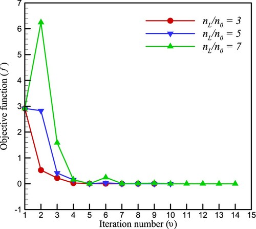
Table 1. Effects of the conduction-radiation parameter on the estimated parameters for the different gradient of refractive index profiles, with $\omega =0.8,{\tau }_L=0.1$ and different measurement error values.

Exact value		$n_0=1,n_L=3$	$n_0=1,n_L=5$	$n_0=1,n_L=7$
Initial guess		$n_0=1.5,n_L=2.5$	$n_0=1.5,n_L=2.5$	$n_0=1.5,n_L=2.5$
$N_{cr}=1.00$	$\eta =0\mathrm{\%}$	$n_0=1.0000,n_L=3.0000$	$n_0=0.9999,n_L=5.0000$	$n_0=0.9944,n_L=6.9988$
	$\eta =1\mathrm{\%}$	$n_0=1.0004,n_L=3.0013$	$n_0=0.9989,n_L=4.9946$	$n_0=1.0039,n_L=7.0195$
	$\eta =3\mathrm{\%}$	$n_0=0.9927,n_L=2.9787$	$n_0=1.0097,n_L=5.0509$	$n_0=0.9923,n_L=6.9553$
	$\eta =5\mathrm{\%}$	$n_0=0.9880,n_L=2.9650$	$n_0=0.9980,n_L=4.9903$	$n_0=0.9943,n_L=6.9670$
$N_{cr}=0.10$	$\eta =0\mathrm{\%}$	$n_0=1.0000,n_L=3.0000$	$n_0=0.9999,n_L=5.0000$	$n_0=0.9996,n_L=6.9999$
	$\eta =1\mathrm{\%}$	$n_0=1.0014,n_L=3.0043$	$n_0=0.9983,n_L=4.9917$	$n_0=0.9795,n_L=7.0095$
	$\eta =3\mathrm{\%}$	$n_0=1.0152,n_L=3.0458$	$n_0=0.9938,n_L=4.9683$	$n_0=0.9989,n_L=6.9887$
	$\eta =5\mathrm{\%}$	$n_0=0.9808,n_L=2.9419$	$n_0=1.0094,n_L=5.0470$	$n_0=1.0065,n_L=7.0478$
$N_{cr}=0.01$	$\eta =0\mathrm{\%}$	$n_0=1.0000,n_L=3.0000$	$n_0=1.0000,n_L=5.0000$	$n_0=1.0000,n_L=7.0000$
	$\eta =1\mathrm{\%}$	$n_0=0.9977,n_L=2.9930$	$n_0=1.0014,n_L=5.0071$	$n_0=1.0018,n_L=7.0121$
	$\eta =3\mathrm{\%}$	$n_0=1.0042,n_L=3.0125$	$n_0=0.9982,n_L=4.9911$	$n_0=0.9935,n_L=6.9562$
	$\eta =5\mathrm{\%}$	$n_0=1.0157,n_L=3.0471$	$n_0=1.0029,n_L=5.0143$	$n_0=0.9918,n_L=6.9447$

In the following, we examine the influence of optical thickness on the estimation of unknown parameters. For this case, three linear refractive index profiles are considered. The results are shown in Table 2, in the presence of various values of $\eta$. As indicated in Table 2, it is clear that the CGM has a remarkable ability to estimate unknown parameters, even for noisy data.

Table 2. Effects of optical thickness on the estimated parameters for the different gradient of refractive index profiles, with $\omega =0.8,N_{cr}=0.1$ and different measurement error values.

Exact value		$n_0=1,n_L=3$	$n_0=1,n_L=5$	$n_0=1,n_L=7$
Initial guess		$n_0=1.5,n_L=2.5$	$n_0=1.5,n_L=2.5$	$n_0=1.5,n_L=2.5$
${\tau }_L=1.00$	$\eta =0\mathrm{\%}$	$n_0=1.0000,n_L=3.0000$	$n_0=1.0000,n_L=5.0000$	$n_0=1.0000,n_L=7.0000$
	$\eta =1\mathrm{\%}$	$n_0=1.0023,n_L=3.0068$	$n_0=1.0021,n_L=5.0097$	$n_0=1.0045,n_L=7.0257$
	$\eta =3\mathrm{\%}$	$n_0=1.0021,n_L=3.0064$	$n_0=1.0031,n_L=5.0156$	$n_0=0.9845,n_L=6.9045$
	$\eta =5\mathrm{\%}$	$n_0=0.9969,n_L=2.9909$	$n_0=0.9998,n_L=4.9990$	$n_0=1.0098,n_L=7.0601$
${\tau }_L=0.10$	$\eta =0\mathrm{\%}$	$n_0=1.0000,n_L=3.0000$	$n_0=1.0000,n_L=5.0000$	$n_0=1.0000,n_L=7.0000$
	$\eta =1\mathrm{\%}$	$n_0=1.0069,n_L=3.0208$	$n_0=0.9999,n_L=4.9994$	$n_0=1.0029,n_L=7.0202$
	$\eta =3\mathrm{\%}$	$n_0=0.9924,n_L=2.9771$	$n_0=1.0042,n_L=5.0208$	$n_0=1.0082,n_L=7.0572$
	$\eta =5\mathrm{\%}$	$n_0=0.9958,n_L=2.9873$	$n_0=0.9980,n_L=4.9900$	$n_0=1.0137,n_L=7.0956$
${\tau }_L=0.01$	$\eta =0\mathrm{\%}$	$n_0=1.0000,n_L=3.0000$	$n_0=1.0000,n_L=5.0000$	$n_0=1.0000,n_L=7.0000$
	$\eta =1\mathrm{\%}$	$n_0=0.9981,n_L=2.9943$	$n_0=1.0027,n_L=5.0131$	$n_0=1.0062,n_L=7.0375$
	$\eta =3\mathrm{\%}$	$n_0=1.9933,n_L=2.9797$	$n_0=0.9987,n_L=4.9935$	$n_0=0.9928,n_L=6.9448$
	$\eta =5\mathrm{\%}$	$n_0=0.9949,n_L=2.9844$	$n_0=0.9943,n_L=4.9713$	$n_0=1.0299,n_L=7.2032$

Now, the effect of isotropic scattering is examined by solving the inverse problem with four cases with different values of single scattering albedo, $\omega$. The results for different values of measurement errors are shown in Table 3. The results show that the scattering has no significant effect on the estimation of boundary refractive indices.

Table 3. Effects of scattering on the estimated parameters for the different gradient of refractive index profiles, with ${\tau }_L=0.1,N_{cr}=0.1$ and different measurement error values.

Exact value		$n_0=1,n_L=3$	$n_0=1,n_L=5$	$n_0=1,n_L=7$
Initial guess		$n_0=1.5,n_L=2.5$	$n_0=1.5,n_L=2.5$	$n_0=1.5,n_L=2.5$
$\omega =0.2$	$\eta =0\mathrm{\%}$	$n_0=1.0000,n_L=3.0000$	$n_0=1.0000,n_L=5.0000$	$n_0=1.0036,n_L=7.0000$
	$\eta =1\mathrm{\%}$	$n_0=0.9956,n_L=2.9867$	$n_0=1.0028,n_L=5.0138$	$n_0=1.0034,n_L=7.0197$
	$\eta =3\mathrm{\%}$	$n_0=1.0051,n_L=3.0151$	$n_0=1.0040,n_L=5.0197$	$n_0=1.0037,n_L=7.0134$
	$\eta =5\mathrm{\%}$	$n_0=1.0031,n_L=3.0093$	$n_0=0.9880,n_L=4.9406$	$n_0=0.9958,n_L=6.9481$
$\omega =0.5$	$\eta =0\mathrm{\%}$	$n_0=1.0000,n_L=3.0000$	$n_0=1.0000,n_L=5.0000$	$n_0=1.0043,n_L=7.0001$
	$\eta =1\mathrm{\%}$	$n_0=0.9992,n_L=2.9975$	$n_0=1.0032,n_L=5.0159$	$n_0=0.9988,n_L=6.9766$
	$\eta =3\mathrm{\%}$	$n_0=1.0020,n_L=3.0060$	$n_0=1.0029,n_L=5.0143$	$n_0=1.0060,n_L=6.9960$
	$\eta =5\mathrm{\%}$	$n_0=1.0344,n_L=3.1029$	$n_0=1.0102,n_L=5.0502$	$n_0=1.0616,n_L=6.9853$
$\omega =0.8$	$\eta =0\mathrm{\%}$	$n_0=1.0000,n_L=3.0000$	$n_0=1.0000,n_L=5.0000$	$n_0=1.0325,n_L=7.0013$
	$\eta =1\mathrm{\%}$	$n_0=0.9974,n_L=2.9921$	$n_0=0.9995,n_L=4.9971$	$n_0=1.0100,n_L=7.0046$
	$\eta =3\mathrm{\%}$	$n_0=1.0176,n_L=3.0527$	$n_0=1.0018,n_L=5.0086$	$n_0=1.0100,n_L=7.0046$
	$\eta =5\mathrm{\%}$	$n_0=1.0071,n_L=3.0211$	$n_0=0.9923,n_L=4.9616$	$n_0=0.9928,n_L=6.9409$
$\omega =1.0$	$\eta =0\mathrm{\%}$	$n_0=1.0000,n_L=3.0000$	$n_0=1.0000,n_L=5.0000$	$n_0=1.0037,n_L=7.0002$
	$\eta =1\mathrm{\%}$	$n_0=1.0014,n_L=3.0042$	$n_0=0.9978,n_L=4.9889$	$n_0=1.0045,n_L=6.9980$
	$\eta =3\mathrm{\%}$	$n_0=0.9988,n_L=2.9964$	$n_0=0.9938,n_L=4.9686$	$n_0=1.0090,n_L=7.0258$
	$\eta =5\mathrm{\%}$	$n_0=1.0144,n_L=3.0431$	$n_0=0.9921,n_L=4.9606$	$n_0=1.0126,n_L=7.0740$

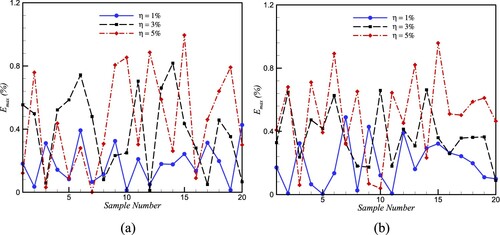
The effects of random errors in measured data are investigated by comparing the maximum relative error for 20 sample runs with different random errors. The inverse approach is used to reconstruct the refractive index profile of Equation (30b), with $n_0=1,n_L=3$. Observing Figure 7, we recognize that by increasing the measurement error, $\eta$, the maximum relative error is increased. However, for the worst situation, the maximum error for highly noisy data is less than 1%, which is an excellent approximation for engineering applications.

Figure 7. The effect of different values of measurement error for 20 sample runs on the estimation of unknown parameters of (a) $n_0$, (b) $n_L$.

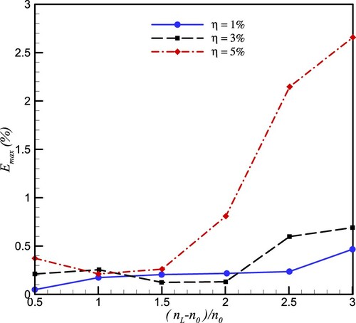
In order to investigate the effect of the gradient of refractive index profile, $(n_l-n_0)/n_0$, we consider six linear refractive index profiles, Equation (30b), with $n_0=1$ and different values for $n_L$. The inverse problem is solved for each refractive index profile for 20 random errors. The maximum relative errors are compared in Figure 8. As seen in Figure 8, the relative error is increased by increasing the gradient of the refractive index. This effect was predictable because when the gradient of the refractive index profile is increased, the medium effects are growth. However, for low values of measurement error ($\eta =1\mathrm{\%},3\mathrm{\%}$), the relative error is small. In other words, for the low values of measurement errors, the influence of the gradient of the refractive index is negligible.

Figure 8. The effect of the refractive index gradient on the maximum error of retrieved unknown parameters for different values of measurement errors.

9. Conclusion

We developed an efficient and accurate approach for inverse estimation of temperature-dependent refractive index profile in conductive-radiative media. The radiative transfer equation was solved by the discrete ordinates method, and the solution of the energy equation was obtained by the finite volume method. The inverse problem was formulated as a minimization problem which was solved by the conjugate gradient method. The accuracy of the direct problem was examined by comparing the results with a benchmark problem. The comparison of temperature-dependent refractive index with spatially dependent refractive index showed that ignoring the effects of temperature on refractive index causes a significant error in the analysis of heat transfer in conductive-radiative media with the variable refractive index. The linear temperature-dependent profile of the refractive index was reconstructed successfully, even for noisy data in measurement data. However, the method may be extended for reconstruction of non-linear profiles of refractive index. The effects of the conduction-radiation parameter, optical thickness, and single scattering albedo were investigated for different values of measurement errors. The results indicated that the accuracy of the inverse solution is decreased by increasing the measurement error, especially for high-gradient profiles of refractive index. However, the accuracy is still good for engineering applications. The inverse method is currently in progress to be extended to nonlinear refractive index profiles.

Disclosure statement

No potential conflict of interest was reported by the author(s).

References

- Born M, Wolf E. Principles of optics. 7th ed. Cambridge: Cambridge University Press; 1999.
- Mishra SC, Kim MY, Das R, et al. Lattice Boltzmann method applied to the analysis of transient conduction-radiation problems in a cylindrical medium. Numer Heat Transf Part A. 2009;56(1):42–59. DOI:https://doi.org/10.1080/10407780903107162.
- Ben-Abdallah P, Le Dez V. Radiative flux field inside an absorbing–emitting semi-transparent slab with variable spatial refractive index at radiative conductive coupling. J Quant Spectrosc Radiat Transf. 2000;67(2):125–137. DOI:https://doi.org/10.1016/S0022-4073(99)00200-9.
- Huang Y, Xia XL, Tan HP. Temperature field of radiative equilibrium in a semi-transparent slab with a linear refractive index and gray walls. J Quant Spectrosc Radiat Transf. 2002;74(2):249–261. DOI:https://doi.org/10.1016/S0022-4073(01)00238-2.
- Tan HP, Huang Y, Xia XL. Solution of radiative heat transfer in a semitransparent slab with an arbitrary refractive index distribution and diffuse gray boundaries. Int J Heat Mass Transf. 2003;46(11):2005–2014. DOI:https://doi.org/10.1016/S0017-9310(02)00502-1.
- Liu LH. Discrete curved ray-tracing method for radiative transfer in an absorbing–emitting semitransparent slab with variable spatial refractive index. J Quant Spectrosc Radiat Transf. 2004;83(2):223–228. DOI:https://doi.org/10.1016/S0022-4073(02)00294-7.
- Xia XL, Huang Y, Zhang XB. Simultaneous radiation and conduction heat transfer in a graded index semitransparent slab with gray boundaries. Int J Heat Mass Transf. 2002;45(13):2673–2688. DOI:https://doi.org/10.1016/S0017-9310(01)00367-2.
- Zhu KY, Huang Y, Wang J. Curved ray tracing method for one-dimensional radiative transfer in the linear-anisotropic scattering medium with graded index. J Quant Spectrosc Radiat Transf. 2011;112(3):377–383. DOI:https://doi.org/10.1016/j.jqsrt.2010.09.005.
- Liu LH. Finite element solution of radiative transfer across a slab with variable spatial refractive index. Int J Heat Mass Transf. 2005;48(11):2260–2265. DOI:https://doi.org/10.1016/j.ijheatmasstransfer.2004.12.045.
- Liu LH. Least-squares finite element method for radiation heat transfer in graded index medium. J Quant Spectrosc Radiat Transf. 2007;103(3):536–544. DOI:https://doi.org/10.1016/j.jqsrt.2006.07.005.
- Liu LH, Liu LJ. Discontinuous finite element method for radiative heat transfer in semitransparent graded index medium. J Quant Spectrosc Radiat Transf. 2007;105(3):377–387. DOI:https://doi.org/10.1016/j.jqsrt.2006.11.017.
- Wang CH, Feng YY, Yue K, et al. Discontinuous finite element method for combined radiation-conduction heat transfer in participating media. Int Commun Heat Mass Transf. 2019;108:104287. DOI:https://doi.org/10.1016/j.icheatmasstransfer.2019.104287.
- Liu LH. Finite volume method for radiation heat transfer in graded index medium. J Thermophys Heat Transf. 2006;20(1):59–66. DOI:https://doi.org/10.2514/1.12459.
- Asllanaj F, Fumeron S. Modified finite volume method applied to radiative transfer in 2D complex geometries and graded index media. J Quant Spectrosc Radiat Transf. 2010;111(2):274–279. DOI:https://doi.org/10.1016/j.jqsrt.2009.06.019.
- Liu LH. Meshless method for radiation heat transfer in graded index medium. Int J Heat Mass Transf. 2006;49(1–2):219–229. DOI:https://doi.org/10.1016/j.ijheatmasstransfer.2005.07.013.
- Wang CA, Tan JY. One-dimensional transient radiative transfer in complex semitransparent medium by meshless method. J Thermophys Heat Transf. 2015;29(3):610–619. DOI:https://doi.org/10.2514/1.T4266.
- Sun YS, Li BW. Spectral collocation method for transient combined radiation and conduction in an anisotropic scattering slab with graded index. ASME J Heat Transf. 2010;132(5):052701. DOI:https://doi.org/10.1115/1.4000444.
- Ma J, Sun YS, Li BW. Completely spectral collocation solution of radiative heat transfer in an anisotropic scattering slab with a graded index medium. ASME J Heat Transf. 2014;136(1):012701. DOI:https://doi.org/10.1115/1.4024990.
- Krishna NA, Mishra SC. Discrete transfer method applied to radiative transfer in a variable refractive index semitransparent medium. J Quant Spectrosc Radiat Transf. 2006;102(3):432–440. DOI:https://doi.org/10.1016/j.jqsrt.2006.02.024.
- Hosseini Sarvari SM. A new approach to solve the radiative transfer equation in plane-parallel semitransparent media with variable refractive index based on the discrete transfer method. Int Commun Heat Mass Transf. 2016;78:54–59. DOI:https://doi.org/10.1016/j.icheatmasstransfer.2016.08.017.
- Hosseini Sarvari SM. Solution of multi-dimensional radiative heat transfer in graded index media using the discrete transfer method. Int J Heat Mass Transf. Sept. 2017;112:1098–1112. DOI:https://doi.org/10.1016/j.ijheatmasstransfer.2017.05.037.
- Mishra SC, Krishna NA, Gupta N, et al. Combined conduction and radiation heat transfer with variable thermal conductivity and variable refractive index. Int J Heat Mass Transf. 2008;51(1–2):83–90. DOI:https://doi.org/10.1016/j.ijheatmasstransfer.2007.04.018.
- Lemonnier D, Le Dez V. Discrete ordinates solution of radiative transfer across a slab with variable refractive index. J Quant Spectrosc Radiat Transf. 2002;73(2–5):195–204. DOI:https://doi.org/10.1016/S0022-4073(01)00222-9.
- Hosseini Sarvari SM. Variable discrete ordinates method for radiation transfer in plane-parallel semi-transparent media with variable refractive index. J Quant Spectrosc Radiat Transf. 2017;199:36–44. DOI:https://doi.org/10.1016/j.jqsrt.2017.05.018.
- Li HY. Estimation of thermal properties in combined conduction and radiation. Int J Heat Mass Transf. 1999;42(3):565–572. DOI:https://doi.org/10.1016/S0017-9310(98)00146-X.
- Verma S, Balaji C. Multi-parameter estimation in combined conduction–radiation from a plane parallel participating medium using genetic algorithms. Int J Heat Mass Transf. 2007;50(9–10):1706–1714. DOI:https://doi.org/10.1016/j.ijheatmasstransfer.2006.10.045.
- Das R, Mishra SC, Uppaluri R. Multiparameter estimation in a transient conduction-radiation problem using the lattice Boltzmann method and the finite-volume method coupled with the genetic algorithms. Numerical Heat Transf, Part A. 2008;53(12):1321–1338. DOI:https://doi.org/10.1080/10407780801959649.
- Das R, Mishra SC, Ajithb M, et al. Simultaneous reconstruction of thermal field and retrieval of parameters in a cylindrical enclosure. Numerical Heat Transf, Part A. 2008;54(10):983–998. DOI:https://doi.org/10.1080/10407780802473608.
- Das R, Mishra SC, Ajithb M, et al. An inverse analysis of a transient 2-D conduction–radiation problem using the lattice Boltzmann method and the finite volume method coupled with the genetic algorithm. J Quant Spectrosc Radiat Transf. 2008;109(11):2060–2077. DOI:https://doi.org/10.1016/j.jqsrt.2008.01.011.
- Das R, Mishra SC, Uppaluri R. Retrieval of thermal properties in a transient conduction–radiation problem with variable thermal conductivity. Int J Heat Mass Transf. 2009;52(11–12):2749–2758. DOI:https://doi.org/10.1016/j.ijheatmasstransfer.2008.12.009.
- Das R, Mishra SC, Uppaluri R. Inverse analysis applied to retrieval of parameters and reconstruction of temperature field in a transient conduction-radiation heat transfer problem involving mixed boundary conditions. Int Commun Heat Mass Transf. 2010;37(1):52–57. DOI:https://doi.org/10.1016/j.icheatmasstransfer.2009.07.016.
- Ajith M, Das R, Uppaluri R, et al. Optimization of heat fluxes on the heater and the design surfaces of a radiating-conducting medium. Numerical Heat Transf Part A. 2009;56(10):846–860. DOI:https://doi.org/10.1080/10407780903423841.
- Ajith M, Das R, Uppaluri R, et al. Boundary surface heat fluxes in a square enclosure with an embedded design element. J Thermophys Heat Transf. 2012;24(4):845–849. DOI:https://doi.org/10.2514/1.49910.
- Zhang B, Qi H, Ren YT, et al. Application of homogenous continuous ant colony optimization algorithm to inverse problem of one-dimensional coupled radiation and conduction heat transfer. Int J Heat Mass Transf. 2013;66:507–516. DOI:https://doi.org/10.1016/j.ijheatmasstransfer.2013.07.054.
- Qi H, Niu CY, Gong S, et al. Application of the hybrid particle swarm optimization algorithms for simultaneous estimation of multi-parameters in a transient conduction–radiation problem. Int J Heat Mass Transf. 2015;83:428–440. DOI:https://doi.org/10.1016/j.ijheatmasstransfer.2014.12.022.
- Sun SC, Qi H, Ren YT, et al. Improved social spider optimization algorithms for solving inverse radiation and coupled radiation-conduction heat transfer problems. Int Commun Heat Mass Transf. 2017;87:132–146. DOI:https://doi.org/10.1016/j.icheatmasstransfer.2017.07.010.
- Wen S, Qi H, Ren YT, et al. Solution of inverse radiation-conduction problems using a Kalman filter coupled with the recursive least–square estimator. Int J Heat Mass Transf. 2017;111:582–592. DOI:https://doi.org/10.1016/j.ijheatmasstransfer.2017.04.017.
- Liu LH. Inverse radiative problem in semitransparent slab with variable spatial refractive index. J Thermophys Heat Transf. 2004;18(3):410–412. DOI:https://doi.org/10.2514/1.5757.
- Namjoo A, Hosseini Sarvari SM, Behzadmehr A, et al. Inverse radiation problem of temperature distribution in one-dimensional isotropically scattering participating slab with variable refractive index. J Quant Spectrosc Radiat Transf. 2009;110(8):491–505. DOI:https://doi.org/10.1016/j.jqsrt.2009.01.034.
- Khayyam S, Hosseini Sarvari SM. Inverse estimation of thermal properties in a semitransparent graded index medium with radiation-conduction heat transfer. ASME J Heat Transf. 2018;140(9):092701. DOI:https://doi.org/10.1115/1.4039992.
- Namjoo A, Hosseini Sarvari SM, Behzadmehr A. Simultaneous estimation of source and refractive index distributions in a one-dimensional absorbing, emitting and scattering graded index medium. Proceedings of Computational Thermal Radiation in Participating Media III (Eurotherm83), April 15–17, Lisbon, Portugal; 2009.
- Namjoo A, Hosseini Sarvari SM, Lemonnier D, et al. Estimation of arbitrary refractive index distribution in a one-dimensional semitransparent graded index medium. Proceedings of 6th International Symposium on Radiative Transfer, June 13–19, Antalya, Turkey; 2010.
- Wei LY, Qi H, Ren YT, et al. Application of stochastic particle swarm optimization algorithm to determine the graded refractive index distribution in participating media. Infrared Phys Technol. 2016;79:74–84. DOI:https://doi.org/10.1016/j.infrared.2016.07.024.
- Wei LY, Qi H, Ren YT, et al. Multi-parameter estimation in semitransparent graded-index media based on coupled optical and thermal information. Int J Therm Sci. 2017;113:116–129. DOI:https://doi.org/10.1016/j.ijthermalsci.2016.11.018.
- Howell JR, Menguc MP, Siegel R. Thermal radiation heat transfer. 6th ed. New York (NY): Taylor and Francis; 2015.
- Patankar SV. Numerical heat transfer and fluid flow. 1st ed. New York (NY): CRC Press; 1980.
- Ozisik MN, Orlande HRB. Inverse heat transfer. New York (NY): Taylor and Francis; 2000.