Inference for the neighbourhood inequality index

ABSTRACT

The neighborhood inequality (NI) index measures aspects of spatial inequality in the distribution of incomes within a city. It is a population average of the normalized income gap between each individual’s income (observed at a given location in the city) and the incomes of the neighbours located within a certain distance range. The approach overcomes the modifiable areal units problem affecting local inequality measures. This paper provides minimum bounds for the NI index standard error and shows that unbiased estimators can be identified under fairly common hypothesis in spatial statistics. Results from a Monte Carlo study support the relevance of the approximations. Rich income data are then used to infer about trends of NI in Chicago, IL, over the last 35 years.

KEYWORDS:

• individual neighbourhood
• variogram
• ratio measures
• variance approximation
• income
• US Census and American Community Survey (ACS)

JEL:

• C12
• C46
• D63
• R23

INTRODUCTION

The importance of regional disparities for economic development, social and political cohesion is well established in the literature (Doran et al., 2018). The increasing inequality pattern registered in the United States in the last few decades seems also to be replicated at a local scale within cities (Baum-Snow & Pavan, 2013; Chetty & Hendren, 2018; Moretti, 2013). Income inequalities that arise from differences across neighbourhoods, understood as areal units defined by an exogenous partition of the urban space, have received substantial attention in the literature (Jargowsky, 1997; Massey & Eggers, 1990; Reardon & Bischoff, 2011; Watson, 2009). Less evidence is available about the extent and dynamics of income inequality within the neighbourhood (relevant contributions are Dawkins, 2007; Hardman & Ioannides, 2004; Kim & Jargowsky, 2009; Shorrocks & Wan, 2005; and Wheeler & La Jeunesse, 2008). The degree of inequality within the neighbourhood of residence has been found to have an independent effect on important dimensions of quality of life, such as labour market attachment (Conley & Topa, 2002), well-being (Ludwig et al., 2012), health (Chetty et al., 2016; Ludwig et al., 2011, 2013) and intergenerational mobility (Andreoli & Peluso, 2018).

Existing approaches to the measurement of inequality within neighbourhoods rely on the exogenous partition of the urban space into areal units, and are hence exposed to the modifiable areal unit problem (MAUP) (Openshaw, 1983; Wong, 2009). The MAUP can be mitigated by addressing neighbourhood inequality across contiguous areas (Chakravorty, 1996; Shorrocks & Wan, 2005) or among neighbours in selected clusters (Hardman & Ioannides, 2004). Andreoli and Peluso (2018) suggest a class of local inequality measures based on the notion of individual neighbourhood (Galster, 2001), assuming spatial continuity in the underlying income distribution. A new neighborhood inequality (NI) index is obtained following two steps of aggregation of spatial income heterogeneity recorded in individual neighbourhoods. First, inequality is assessed within each individual neighbourhood of a fixed (arbitrary) size. An individual neighbourhood in location $s$ gathers all income units located within the circular region of given size centred on $s$, and it may overlap with other individual neighbourhoods of similar size but centred on different locations. Second, the resulting values of inequality within individual neighbourhoods are aggregated across the relevant population. The approach guarantees robustness vis-à-vis the MAUP, insofar individual neighbourhoods depend exclusively on the spatial arrangements of incomes on the map but do not rely on a specific organization of the space.

Using census and American Community Survey (ACS) data from American MSAs, Andreoli and Peluso (2018) find that neighbourhood inequality is (1) high and close to citywide inequality, even when the neighbourhood size is < 1 mile in range; (2) on the rise since the 1980s; and (3) displays similar patterns across cities. The NI index estimates may be biased by measurement error and by the sampling design of spatial data, whereas bias cannot be effectively dealt with without an appropriate inference strategy.

In this paper, we derive minimum bounds for the standard error (SE) of the NI index and use these bounds to infer about robust changes in NI. We use some properties of the ratio estimators in Goodman and Hartley (1958) to derive bounds for the NI index variance when the data-generating process is not i.i.d., accommodating for the possibility of spatial dependence. We assume that the process is continuous in nature and relies exclusively on information about income levels and their geocoded location. We then show (in the second and third sections) that under fairly common assumptions in spatial statistics, the estimators of the NI index SE are identified by moments of the spatial income distribution and by the variogram, a measure of spatial dependence of the data (Matheron, 1963). A simulation study (in the fourth section) confirms the qualities of the SE estimator proposed here. The fifth section infers about changes in NI in Chicago, IL, where we find robust statistical support for rising neighbourhood inequality irrespectively of the chosen size of individual neighbourhoods. The sixth section concludes.

MEASURING INEQUALITY IN THE NEIGHBOURHOOD

NI index and the related literature

Consider a population of $n\ge 3$ individuals, indexed by $i=1,\dots ,n$. Let $y_i$ be the income of individual $i$ and $y=\left(y_1,y_2,\dots ,y_n\right)$ the sample income distribution with average $\mu >0$. Information on incomes comes with information about their location on the city map (non-stochastic). An individual neighbourhood $d_i$ gathers $n_{id}$ individuals living in the circular region of ray $d$ centred on location $i$. If each individual occupies a separate location, there would be as many different individual neighbourhoods as individuals in the city. Each individual neighbourhood is characterized by an average income ${\mu }_{id}=\sum _{j\in d_i}{y}_j/n_{id}$, while ${\mathrm{\Delta }}_i\left(y,d\right)=\left(1/{\mu }_{id}\right)\sum _{j\in d_i}\left(\left|y_{i-}{y}_j\right|/n_{id}\right)$ is a normalized measure of the average gap between $i$’s income and that of her neighbours. The NI index measures the degree of inequality in the average individual neighbourhood. It is defined as:(1) $NI\left(y,d\right)=\frac{1}{2}\sum _{i=1}^n\frac{1}{n}{\mathrm{\Delta }}_i\left(y,d\right).$(1) The NI index depends on $d$, a parameter chosen by the researcher. The plot of $NI\left(y,d\right)$ against $d$ defines a NI curve. The curve is expected to be close to the origin when $d$ tends to zero (individual neighbourhoods are very small), remaining low when sample units are spatially clustered by income. When $d$ reaches the size of the city, each individual neighbourhood spans the whole city. In this case, neighbourhood inequality converges to citywide inequality measured by the Gini index and the NI curve is flat.

Alternative approaches to spatial inequality within (Shorrocks & Wan, 2005; Wheeler & La Jeunesse, 2008) and across (Iceland & Hernandez, 2017; Reardon & Bischoff, 2011) areal units (such as regions, counties, census tracts, etc.) have been discussed in the literature. These approaches are subject to the MAUP (Openshaw, 1983; Wong, 2009), that is, they are not robust to the zonation effect, due to the administrative partition of space (for instance, by census tracts or school districts), or to the subsequent way of scaling it (for instance, by block groups or by zip codes). The example in Figure 1 illustrates the implications of these effects for spatial inequality. Each panel shows the spatial distribution of rich (black dots) and poor (circles) individuals. The administrative partition of the stylized city is induced by vertical and horizontal lines. As a consequence of the zonation effect (Figure 1 (A)), spatial inequality measures may reverse the ranking of the two cities by just changing the design of the administrative partition (i.e., replacing the horizontal lines by the vertical ones artificially minimizes inequality within neighbourhoods, inhabited by same-income individuals, and maximizes inequality between neighbourhoods). As a consequence of the scaling effect (Figure 1 (B)), large discontinuities in spatial inequality evaluation may occur in response to minor refinements of the neighbourhoods’ partition. In the upper diagram of Figure 1(B), each neighbourhood displays the same inequality as in the city. In the bottom diagram, inequality within neighbourhoods is eliminated by virtue of a finer partition obtained by drawing two additional vertical lines. If, instead, the finer partition was obtained by drawing horizontal lines, then the opposite situation (high inequality within the neighbourhood) would have emerged.

Figure 1. Scaling and zonation effects on neighbourhood inequality.

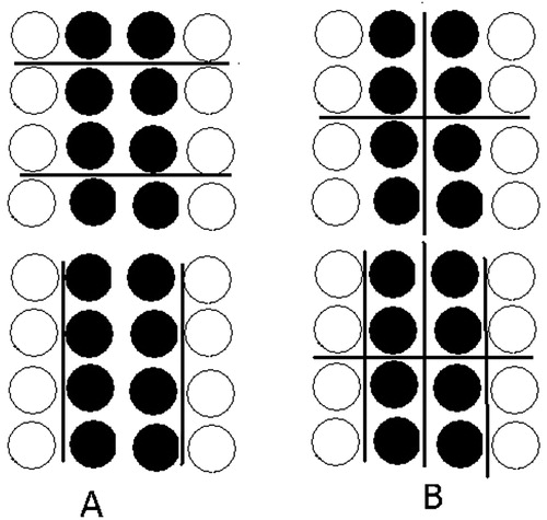
The NI index overcomes the MAUP by treating the spatial distribution of income as continuous and by using individual neighbourhoods to avoid the zonation issues. Furthermore, scaling is also controlled for by the levels of the distance threshold $d$, so that evaluations only depend on the actual distribution of incomes in space. These properties guarantee that the NI index ranks as equivalent the two panels A and B in Figure 1.

Individual neighbourhoods have been used in the analysis of segregation in space (Clark et al., 2015; Galster, 2001), in networks (Echenique & Fryer, 2007), across housing units (Hardman & Ioannides, 2004) or across time (Biondi & Qeadan, 2008). Chakravorty (1996) applied the notion of individual neighbourhood to organizational units to develop a neighborhood disparity measure (ND), which is a normalized average of the difference between the income observed in each areal unit and the average income of neighbouring parcels.

The NI index is instead related to the Gini index of inequality and develops on pairwise income comparisons within individual neighbourhoods. Following Pyatt (1976), the NI index can be interpreted as the expected (relative) income gain that a randomly chosen urban resident would experience if her income was exchanged with those of her neighbours located within a ray of length $d$. Differently from traditional decomposable inequality measures, the NI index considers a multidimensional distribution of individual income observations alongside individual geographical locations. The two ingredients are combined through the individual neighbourhoods. This allows establishing a methodological bridge with geostatistics.

Statistical properties of the NI index

Consider a spatially continuous process $\left\{Y_s:s=1,\dots ,n\right\}$ where $s\in \mathcal{S}$ is one location on the random field and $n$ is the total number of locations. The process is jointly distributed as ${\mathcal{F}}_{\mathcal{S}}$ and may represent, for instance, the data-generating process underlying the spatial distribution of incomes across locations in a city. The joint distribution function ${\mathcal{F}}_{\mathcal{S}}$ combines information about the marginal income distributions in each location and the degree of spatial dependence of incomes on $\mathcal{S}$. In the analysis, locations on $\mathcal{S}$ are non-random and the process is defined conditionally on $\mathcal{S}$. Through geolocalization, it is possible to compute the distance ‘$\left||.|\right|$’ between two generic locations $s,v\in \mathcal{S}$, which we denote $\left|\left|s-v\right|\right|\le d$ or equivalently $v\in d_s$, which denotes the set of locations located within a range $d$ from $s$. The cardinality of $d_s$ is $n_{d_s}$. The observed spatial income distribution $y$ (alongside geographical coordinates of the income observations) is a particular draw from ${\mathcal{F}}_{\mathcal{S}}$, where only one income realization is observed in any location $s$.

The NI index of the spatial process ${\mathcal{F}}_{\mathcal{S}}$ can be written in terms of first-order moments of the random variables $Y_s$ as follows:(2) $NI\left({\mathcal{F}}_{\mathcal{S}},d\right)=\sum _s\sum _{v\in d_s}\frac{1}{2n{n}_{d_s}}\frac{E\left[\left|Y_s-Y_v\right|\right]}{E\left[Y_v\right]}.$(2) The numerator in (2) depends on the extent of spatial dependence displayed by ${\mathcal{F}}_{\mathcal{S}}$. To show this, consider the restrictive yet widely adopted parametric assumption that $Y_i$ follows a linear SAR model with $Y=\mathit{\mu }+{\rho }_d{W}_d\cdot \left(Y-\mathit{\mu }\right)+ϵ$, with $Y=(Y_1,\dots ,Y_n{)}^{\mathrm{\prime }}$, where $W_d$ is an $n\times n$ spatial weighting matrix with $w_{ij}=1/n_{d_i}$ if $j\in d_i$ and $w_{ij}=0$ otherwise; $ϵ$ is a column vector of i.i.d. innovations; and $\mathit{\mu }=(\mu ,\dots \mu )$ with the average income. The parameter ${\rho }_d$ measures spatial autocorrelation at distance range $d$ (Moran’s I statistics is often used as an estimator for this correlation; Li et al., 2007). Under standard assumptions (Kelejian & Prucha, 2010), $Y=\mathit{\mu }+(I-{\rho }_d{W}_d{)}^{-1}\cdot ϵ=\mathit{\mu }+S({\rho }_d)\cdot ϵ$, so that $Y_i=\mu +S_i\left({\rho }_d\right)\cdot ϵ$, where $S_i\left({\rho }_d\right)$ is a non-stochastic row vector. Under these circumstances, $E\left[\left|Y_s-Y_v\right|\right]=E\left[\left|S_s\left({\rho }_d\right)\cdot ϵ-S_v\left({\rho }_d\right)\cdot ϵ\right|\right]$ depends on both inequality in the data ($ϵ$) and spatial correlation in the data ($S\left({\rho }_d\right)$), whereas $E\left[Y_v\right]=\mu$.

If incomes $Y_s$ and $Y_v$ are i.i.d. with distribution ${\mathcal{F}}_{\mathcal{S}}$ for any $s,v\in \mathcal{S}$ (i.e., ${\rho }_d=0$ at any $d$), then $NI\left({\mathcal{F}}_{\mathcal{S}},d\right)=E\left[\left|Y_s-Y_v\right|\right]/E\left[Y_v\right]$ ($=E\left[\left|{ϵ}_s-{ϵ}_v\right|\right]/\mu$ under SAR), which coincides with a definition of the Gini index (Muliere & Scarsini, 1989). If, instead, spatial dependence is at stake (typically ${\rho }_d>0$), then the NI index differs from the Gini index and $E\left[\left|Y_s-Y_v\right|\right]$ varies across locations. This quantity cannot be identified from the observation of just one data point in each location. We then introduce additional assumptions about the spatial income process that allow to derive the NI index from the first and second moments of ${\mathcal{F}}_{\mathcal{S}}$.

The first assumption is that ${\mathcal{F}}_{\mathcal{S}}$ displays (second-order) stationarity (Chilès & Delfiner, 2012), that is, $E\left[Y_s\right]=\mu$, $Var\left[Y_s\right]={\sigma }^2$ and $Cov\left[Y_s,Y_v\right]=c\left(\left|\left|v-s\right|\right|\right)=c\left(d\right)$ is isotropic, with $\left|\left|v-s\right|\right|=d$. Under these circumstances, $Var\left[Y_{s+d}-Y_s\right]=E\left[{\left(Y_{s+d}-Y_s\right)}^2\right]=2{\sigma }^2-2c\left(d\right)=2\gamma \left(d\right)$ denotes the variogram of the process at distance range $d$ (Matheron, 1963). The function $2\gamma \left(d\right)$ is informative of the correlation between two random variables that are at a distance $d$ one from the other, insofar $c\left(d\right)={\sigma }^2-\gamma \left(d\right)$. Under stationarity, $2\gamma \left(d\right)\to 0$ as $d$ approaches 0 if the spatial process displays high positive association at small distance ranges. Conversely, $2\gamma \left(d\right)\to 2{\sigma }^2$ when $d$ is sufficiently large, indicating spatial independence. We follow the convention that $s-v=d$ whenever $\left|\left|s-v\right|\right|=d$ (which implies that the process occurs on a transect at neighbourhood level).

The second assumption is that $Y_s$ is Gaussian with mean $\mu$ and variance ${\sigma }^2$. The random variable $\left(Y_{s+d}-Y_s\right)$ is also Gaussian with variance $2\gamma \left(d\right)$, which implies $\left|Y_{s+d}-Y_s\right|$ is folded-normal distributed (Leone et al., 1961) and its first and second moments depend exclusively on the variogram, having expectation $E\left[\left|Y_{s+d}-Y_s\right|\right]=\sqrt{2/\pi Var\left[Y_{s+d}-Y_s\right]}=2\sqrt{\gamma \left(d\right)/\pi }$ and variance $Var\left[\left|Y_{s+d}-Y_s\right|\right]=\left(1-2/\pi \right)2\gamma \left(d\right)$.

Altogether, these assumptions allow to characterize the NI index as a function of the variogram. For given $d$, we consider partitioning the distance spectrum $\left[0,d\right]$ into $B_d$ ordered intervals of size $d/B_d$, and derive the NI index formulation at distance intervals of fixed size. If the size were chosen equal to the minimum distance recorded between locations, then the NI index could be rewritten explicitly as a function of locations. Each interval is denoted by the index $b$ with $b=1,\dots ,B_d$. We further denote with $d_{bi}$ the set of locations at interval $b$ (and thus distant $b\cdot d/B_d$ from $s_i$) within the range $d$ from location $s_i$. The cardinality of this set is $n_{d_{bi}}\le n_{d_i}\le n$. Assuming stationarity of ${\mathcal{F}}_{\mathcal{S}}$ and normality allows to write the $NI$ index as follows:(3) $\begin{array}{rl}NI({\mathcal{F}}_{\mathcal{S}},d)& =\sum _i\sum _{j\in d_i}\frac{1}{2n{n}_{d_i}}\frac{E\left[\right|Y_{s_j}-Y_{s_i}\left|\right]}{\mu }\\ & =\sum _i\sum _{j\in d_i}\frac{1}{2n{n}_{d_i}}\frac{\sqrt{4\gamma \left(\right||s_j-s_i|\left|\right)/\pi }}{\mu }\\ & =\sum _i\frac{1}{n}\sum _{b=1}^{B_d}\frac{n_{d_{bi}}}{n_{d_i}}\sum _{j\in d_{bi}}\frac{1}{2n_{d_{bi}}}\frac{\sqrt{4\gamma (s_i+b-s_i)/\pi }}{\mu }\\ & =\frac{1}{2}\sum _{b=1}^{B_d}\left(\sum _i\frac{n_{d_{bi}}}{n{n}_{d_i}}\right)\frac{\sqrt{4\gamma \left(b\right)/\pi }}{\mu },\end{array}$(3) This result (see also Andreoli & Peluso, 2018) sets out the geostatistics foundations of the NI index by showing that the index is fully characterized by the distribution of locations on the city map (non-stochastic) and the degree of spatial dependence measured by the variogram.¹ Under these assumptions, the index can be understood as an average of a standardized measure of dispersion (the second term in the summation in (3)) taken at different distance thresholds $b$, and weighted by the population on the random field located on the average individual neighbourhood of size $d$, a parameter chosen by the researcher. The implications of dropping the normality assumption, widely (often implicitly) adopted in geostatistics analysis, are assessed in a Monte Carlo experiment. For the results, see Appendix C in the supplemental data online.

Discussion

A few remarks are in order. First, the NI index depends both on geographical distance across locations and local income variability, averaged across all individual neighbourhoods while holding distance range fixed. In the presence of positive spatial correlation in incomes, small individual neighbourhoods gather few likely similar income realizations, implying minimal income heterogeneity ($NI\to 0$). When the size of the individual neighbourhood is large, the inequality evaluation tends to include an increasing number of income observations that are spatially unrelated. For large $d$, the variogram coincides with the variance of the stationary process and is constant. Equation (3) shows that the NI index stabilizes on a converging level of inequality when rising $d$, hence rising the weight of locations where incomes are spatially uncorrelated. This level of inequality is the Gini index of the population income distribution.²

A second remark is about the choice of the distance parameter $d$. This parameter’s relative magnitude is contingent to the problem under analysis. When addressing neighbourhood income inequality in an urban context, it makes sense to limit the analysis to well-defined statistical aggregates such as commuting zone or metropolitan statistical areas. The geographical size of these areas is generally well defined by their administrative boundaries, density and commuting time requirements. The interpretation of the NI index, which is grounded on individual neighbourhoods attributable to the residents, is meaningful when $d$ is limited to the boundaries of the city.³ The choice of a limit for a distance parameter may become crucial when analysing spatial inequality within inner cities, thus neglecting edge effects on the NI index and its SE bounds induced by the income distribution across the boundary areas of the city. Appendix D in the supplemental data online investigates more carefully the issue of edge effects.

Third, we stress that the NI index is a measure of inequality which is normalized by an implicit spatial weighting scheme, which we assume to be uniform in (2) and (3). More precisely, each income unit observed within $i$’s individual neighbourhood is weighted $1/n_{d_i}$, whereas individual neighbourhoods are weighted $1/n$. This weighting scheme allows us to capture empirically aspects related to the population size, as well as the population distribution across the data field, which may cluster in dense urban areas, or sprawl in suburbs. The relation between $d$ and $n$ in the population is described by the intensity of the population point process (the concept is formalized, among others, by Diggle, 1985). The local density $n_{d_i}$ is an estimator of the process intensity, which may be a source of bias in the NI index estimates. This bias vanishes when $n$ is large⁴ but may still survive for small values of $d$ (small individual neighbourhoods) if local density is too small. These concerns seem to be of secondary importance for empirical applications of the NI index in the context of urban inequality analysis. One the one hand, urban agglomerates generally display large population size and density at all distance scales. On the other, meaningful estimators of the empirical variogram for (3) should be based on at least 30 pairs of observations (Journel & Huijbregts, 1989, p. 194), thus providing a minimum bound for estimating the NI index at small geographical scale. Additionally, the simulation study by LeSage and Pace (2014) suggests that, at small distance ranges, the exact specification of the weighting scheme is likely irrelevant for addressing spatial variability in the data. These considerations extend to the estimation of the NI variance bounds, also based on the variogram.

VARIANCE BOUNDS FOR THE NI INDEX

Main result

We explore the geostatistics foundations of the NI index to derive empirically tractable bounds for the NI index variance. We denote locations on the random field with $i=1,\dots ,n$, each having non-stochastic weight $w_i\ge 0$ with $w=\sum _i{w}_i$, which might reflect the inverse probability of selection from the population. The underlying process $\mathcal{F}$ is stationary with mean $\mu$ and variance ${\sigma }^2$.

The first implication of the assumptions we consider is that, asymptotically, the random variable ${\mu }_{id}=\sum _{j\in d_i}\left(w_j/\sum _{j\in d_i}{w}_j\right)Y_j$ is equivalent in expectation to $\tilde{\mu }=\sum _i\left(w_i/\sum _i{w}_i\right)Y_i$, with, $E\left[\tilde{\mu }\right]=\mu$. The second implication is that the spatial correlation exhibited by $\mathcal{F}$ is stationary in $d$ and can be represented through the variogram of $\mathcal{F}$, denoted $2\gamma \left(d\right)$.

Our analysis focuses on an asymptotically equivalent version of the weighted NI index of the process distributed as $\mathcal{F}$, that is:(4) $NI\left(\mathcal{F},d\right)=\frac{1}{2\tilde{\mu }}\sum _{i=1}^n\sum _{j\in d_i}\frac{w_i{w}_j}{2w\sum _{j\in d_i}{w}_j}\left|Y_i-Y_j\right|=\frac{1}{2\tilde{\mu }}{\mathrm{\Delta }}_d.$(4) The NI index can thus be expressed as a ratio of two random variables. Asymptotic approximations for the SE of ratios of random variables have been developed by Goodman and Hartley (1958, p. 496). Koop (1964) and Tin (1965) have demonstrated that, under normality, such approximations are minimum variance bounds. We use these results to obtain minimum variance bounds for the NI index in (4) as follows:(5) $\begin{array}{rl}Var\left[NI\left(\mathcal{F},d\right)\right]=& \frac{1}{4n{\mu }^2}Var\left[{\mathrm{\Delta }}_d\right]+\frac{{\left(NI\left(\mathcal{F},d\right)\right)}^2}{n{\mu }^2}Var\left[\tilde{\mu }\right]\\ & -\frac{NI\left(\mathcal{F},d\right)}{n{\mu }^2}Cov\left[{\mathrm{\Delta }}_d,\tilde{\mu }\right]+O\left(n^{-2}\right),\end{array}$(5) where the SE approximation is $S{E}_d=\sqrt{Var\left[NI\left(\mathcal{F},d\right)\right]}$ at any $d$. The approximation converges quickly when the number of locations is large, as it the case in applications based on census micro-data, and holds when income realizations are spatially correlated.⁵ As suggested by Tin (1965), we use plug-in estimators for the SE.

We provide estimators for each of the three addends in (5) under appropriate assumptions. First, we assume that the process $\mathcal{F}$ is stationary with known second moments. Let the positive integer scalars $m,b,b^{\mathrm{\prime }}$ identify non-overlapping intervals of the distance range $d$, and $B$ is the number of such intervals. The variance of $\tilde{\mu }$, $Var\left[\tilde{\mu }\right]$, writes:(6) $\begin{array}{rl}Var\left[\tilde{\mu }\right]& =\sum _i\frac{w_i}{w}\sum _j\frac{w_j}{w}E\left[Y_i{Y}_j\right]-{\mu }^2\\ & =\sum _i\frac{w_i}{w}\sum _{m=1}^B\frac{{\sum }_{j\in d_{mi}}{w}_j}{w}\sum _{j\in d_{mi}}\frac{w_j}{{\sum }_{j\in d_{mi}}{w}_j}c\left(\right||s_i-s_j|\left|\right).\end{array}$(6) (7) $=\sum _{m=1}^B\left(\sum _i\frac{w_i}{w}\frac{{\sum }_{j\in d_{mi}}{w}_j}{w}({\sigma }^2-\gamma (m\left)\right)\right).$(7) (8) $={\sigma }^2-\sum _{m=1}^B\omega \left(m\right)\gamma \left(m\right),$(8) where (8) is obtained from (7) by renaming the weight scores so that $\sum _{m=1}^B\omega \left(m\right)=1$, and by using the definition of the variogram and the fact that $s_j=s_i+m$. The score $\omega (.)$ depends on the density in one given location. In random sampling with uniform weights (i.e. when $w_i=1/n$), this factor reduces to an average of the population $n_{d_{mi}}$ residing in distance segment $m$ from any unit $i$ normalized by the total population, that is:$\omega \left(m\right)=\frac{1}{n}\sum _i\frac{1}{n}{n}_{d_{mi}}.$

The second variance component of (5), $Var\left[{\mathrm{\Delta }}_d\right]$, can be written as follows:$\begin{array}{rl}Var\left[{\mathrm{\Delta }}_d\right]=& \sum _{i=1}^n\sum _{j\in d_i}\frac{w_i{w}_j}{w{\sum }_{j\in d_i}{w}_j}\sum _{\ell =1}^n\sum _{k\in d_{\ell }}\frac{w_{\ell }{w}_k}{w{\sum }_{k\in d_{\ell }}{w}_k}E\left[\left|Y_i-Y_j\right|\left|Y_{\ell }-Y_k\right|\right]\\ & -{\left(\sum _i\frac{w_i}{w}\sum _{j\in d_i}\frac{w_j}{{\sum }_{j\in d_i}{w}_j}E\left[\left|Y_j-Y_i\right|\right]\right)}^2.\end{array}$The first component of $Var\left[{\mathrm{\Delta }}_d\right]$ cannot be further simplified, as the absolute value operator enters the expectation term in a multiplicative way. We assume stationarity and, additionally, normality to be able to simulate the expectation, since the random vector $(Y_j,Y_i,Y_k,Y_{\ell })$ is jointly normally distributed with expectations $(\mu ,\mu ,\mu ,\mu )$ and variance–covariance matrix $Cov\left[\left(Y_j,Y_i,Y_k,Y_{\ell }\right)\right]$, with:$Cov\left[\left(Y_j,Y_i,Y_k,Y_{\ell }\right)\right]=\left(\begin{array}{cccc}{\sigma }^2& c\left(\left|\left|s_j-s_i\right|\right|\right)& c\left(\left|\left|s_j-s_k\right|\right|\right)& c\left(\left|\left|s_j-s_{\ell }\right|\right|\right)\\ & {\sigma }^2& c\left(\left|\left|s_i-s_k\right|\right|\right)& c\left(\left|\left|s_i-s_{\ell }\right|\right|\right)\\ & & {\sigma }^2& c\left(\left|\left|s_k-s_{\ell }\right|\right|\right)\\ & & & {\sigma }^2\end{array}\right).$Denote further that $s_j-s_i=b\ge 0$ and $s_k-s_{\ell }=b^{\mathrm{\prime }}\ge 0$ for the positive integers $b\le B_d$ and $b^{\mathrm{\prime }}\le B_d$. We also take the (unrestrictive) convention that $s_i-s_{\ell }=m$ with $0\le m\le B$. We can hence express the variance–covariance matrix as a function of the variogram:$Cov\left[\left(Y_j,Y_i,Y_k,Y_{\ell }\right)\right]=\left(\begin{array}{cccc}{\sigma }^2& {\sigma }^2-\gamma \left(b\right)& {\sigma }^2-\gamma \left(m+b-b^{\mathrm{\prime }}\right)& {\sigma }^2-\gamma \left(m+b\right)\\ & {\sigma }^2& {\sigma }^2-\gamma \left(m-b^{\mathrm{\prime }}\right)& {\sigma }^2-\gamma \left(m\right)\\ & & {\sigma }^2& {\sigma }^2-\gamma \left(b^{\mathrm{\prime }}\right)\\ & & & {\sigma }^2\end{array}\right).$The expectation $E\left[\left|Y_i-Y_j\right|\left|Y_{\ell }-Y_k\right|\right]$ can be simulated from a large number $S$ (with $S=1,000$) of independent draws $\left(y_{1s},y_{2s},y_{3s},y_{4s}\right)$ with $s=1,\dots ,S$, from the random vector $\left(Y_j,Y_i,Y_k,Y_{\ell }\right)$. The simulated expectation is a function of the variogram parameters $m$, $b$, $b^{\mathrm{\prime }}$ and $d$ and of ${\sigma }^2$. It is denoted $\theta \left(m,b,b^{\mathrm{\prime }},d,{\sigma }^2\right)$ and estimated as follows:$\theta \left(m,b,b^{\mathrm{\prime }},d,{\sigma }^2\right)=\frac{1}{S}\sum _{s=1}^S\left|y_{2s}-y_{1s}|\cdot |y_{4s}-y_{3s}\right|.$

With some algebra, and using the fact that $E\left[\left|Y_{\ell }-Y_i\right|\right]=2\sqrt{\gamma \left(m\right)/\pi }$ for locations $\ell$ and $i$ at distance $m\le B$ one from each other, it is then possible to write the term $Var\left[{\mathrm{\Delta }}_d\right]$ as follows:(9) $\begin{array}{rl}& Var\left[{\mathrm{\Delta }}_d\right]=\sum _{m=1}^B\sum _{b=1}^{B_d}\sum _{b^{\mathrm{\prime }}=1}^{B_d}\omega \left(m,b,b^{\mathrm{\prime }},d\right)\theta \left(m,b,b^{\mathrm{\prime }},d,{\sigma }^2\right)\\ & -4{\left(\sum _{B_d}^m\omega \left(m,d\right)\sqrt{\gamma \left(m\right)/\pi }\right)}^2.\end{array}$(9) In the formula, $\omega \left(m,b,b^{\mathrm{\prime }},d\right)=\sum _i\left(w_i/w\right)\sum _{j\in d_{bi}}\left(w_j/\sum _{j\in d_i}{w}_j\right)\sum _{\ell \in d_{mi}}\left(w_{\ell }/w\right)\sum _{k\in d_{b^{\mathrm{\prime }}\ell }}\left(w_k/\sum _{k\in d_{\ell }}{w}_k\right)$ and $\omega \left(m,d\right)=\sum _i\left(w_i/w\right)\sum _{j\in d_{mi}}\left(w_j/\sum _{j\in d_i}{w}_j\right)$ are calculated as before.

The third component of (5) is the covariance term. It can also be written as a function of the variogram. To show this, we maintain the convention that $s_i-s_{\ell }=m\ge 0$ and $s_j-s_i=b\ge 0$. This gives the following equivalence:(10) $\begin{array}{rl}E\left[\right|Y_j-Y_i\left|Y_{\ell }\right]& =E\left[\right|Y_j{Y}_{\ell }-Y_i{Y}_{\ell }\left|\right]=E\left[Y_j{Y}_{\ell }\right]-E\left[Y_i{Y}_{\ell }\right]-2E[min\{Y_j{Y}_{\ell }-Y_i{Y}_{\ell },0\left\}\right]\\ & =c\left(\right||s_j-s_{\ell }|\left|\right)+{\mu }^2-c\left(\right||s_i-s_{\ell }|\left|\right)-{\mu }^2-2E[min\{Y_j{Y}_{\ell }-Y_i{Y}_{\ell },0\left\}\right]\\ & =\gamma \left(m\right)-\gamma (m+b)-2E[min\{Y_j{Y}_{\ell }-Y_i{Y}_{\ell },0\left\}\right].\end{array}$(10) The expectation $E\left[min\left\{Y_j{Y}_{\ell }-Y_i{Y}_{\ell },0\right\}\right]$ is non-linear in the underlying random variables. Under the Gaussian assumption, the expectation can be simulated from a large number $S$ (with $S=1,000$) of independent draws $\left(y_{1s},y_{2s},y_{3s}\right)$ with $s=1,\dots ,S$, from the random vector$\left(Y_j,Y_i,Y_{\ell }\right)$, which is normally distributed with expectations $\left(\mu ,\mu ,\mu \right)$ and variance–covariance matrix $Cov\left[\left(Y_j,Y_i,Y_{\ell }\right)\right]$. The variance–covariance matrix writes:$Cov\left[\left(Y_j,Y_i,Y_{\ell }\right)\right]=\left(\begin{array}{ccc}{\sigma }^2& {\sigma }^2-\gamma \left(b\right)& {\sigma }^2-\gamma \left(m+b\right)\\ & {\sigma }^2& {\sigma }^2-\gamma \left(m\right)\\ & & {\sigma }^2\end{array}\right)$for given $m$, $b$ and $d$. The resulting simulated expectation is denoted $\phi \left(m,b,d,{\sigma }^2\right)$ and computed as follows:$\phi \left(m,b,d,{\sigma }^2\right)=\frac{1}{S}\sum _{s=1}^{S}min\left\{y_{1s}{y}_{3s}-y_{2s}{y}_{3s},0\right\}.$Based on this result, the covariance term in (5) becomes:(11) $\begin{array}{rll}Cov[{\mathrm{\Delta }}_d,\tilde{\mu }]& =& \sum _i\frac{w_i}{w}\sum _{j\in d_i}\frac{w_j}{\sum _{j\in d_i}{w}_j}\sum _{\ell }\frac{w_{\ell }}{w}E[|Y_j-Y_i|Y_{\ell }]\\ & & -\mu \sum _i\frac{w_i}{w}\sum _{j\in d_i}\frac{w_j}{\sum _{j\in d_i}{w}_j}E[|Y_j-Y_i|]\\ & =& \sum _{m=1}^B\sum _{b=1}^{B_d}\omega (m,b,d)\left[\gamma \left(m\right)-\gamma (m+b)-2\phi (m,b,d,{\sigma }^2)\right]\\ & & -2\mu \sum _{m=1}^{B_d}\omega (m,d)\sqrt{\gamma \left(m\right)/\pi }\end{array}.$(11)

The weights in (11) coincide respectively with $\omega \left(m,b,d\right)={\sum }_i{\displaystyle \frac{w_i}{w}{\sum }_{\ell \in d_{mi}}\frac{w_{\ell }}{w}{\sum }_{j\in d_{bi}}\frac{w_j}{\sum _{j\in d_i}{w}_j}}$ and $\omega \left(m,d\right)={\sum }_i{\displaystyle \frac{w_i}{w}{\sum }_{j\in d_{mi}}\frac{w_j}{\sum _{j\in d_i}{w}_j}.}$

A consistent estimator for the SE, denoted ${\widehat{SE}}_d$, is obtained by plugging into (5) the empirical counterparts of the variogram and the lag-dependent weights, using formulas in (8), (9) and (11). Cressie and Hawkins (1980) provide non-parametric estimators for the variogram that are robust with respect to outliers (in the empirical application, we use the robust spherical variogram model in Cressie, 1985). For details, see Appendix A in the supplemental data online.

Hypothesis testing

The NI index and the implied NI curves can be used to assess patterns and trends of neighbourhood inequality. Various hypotheses are of interest. One concern may be about the extent at which inequality in the average individual neighbourhood of size $d$ is different from citywide inequality measured by the Gini index. The relevant null hypothesis is $H_0^1:NI\left(y,d\right)=G\left(y\right)$ against an unrestricted alternative (reflecting the fact that neighbourhood inequality can be either larger or smaller than citywide inequality). A second concern is that the empirical patterns of neighbourhood inequality are related to the size of individual neighbourhoods. In presence of income sorting, one expects that inequality within neighbourhoods of small size to be, on average, smaller than inequality in neighbourhoods of larger size. Consequently, the NI curve is expected to be increasing in the individual neighbourhood size. The relevant null here is $H_0^2:NI\left(y,d^{\mathrm{\prime }}\right)=NI\left(y,d\right)$ for $d^{\mathrm{\prime }}>d$, to be tested against a restricted alternative. Rejecting both null hypotheses $H_0^1$ and $H_0^2$ gives statistical support for the existence of a neighbourhood component in the urban income distribution.

It is also of interest to study the dynamics of neighbourhood inequality across income distributions $y_t$ and $y_{t^{\mathrm{\prime }}}$. For a given size $d$ of the individual neighbourhood, the relevant null hypothesis is $H_0^3\left(d\right):NI\left(y_t,d\right)=NI\left(y_{t^{\mathrm{\prime }}},d\right)$ against an unrestricted one. An increase or decline in neighbourhood inequality is robust (with respect to the choice of the distance parameter) when it involves a form of dominance in neighbourhood inequality curves: that is, when the NI curves never intersect each other. In this case, the relevant null hypothesis is: $H_0^3:H_0^3\left(d\right)forsomed$ against a constrained alternative $\underset{d}{min}\left\{NI\left(y_t,d\right)-NI\left(y_{t^{\mathrm{\prime }}},d\right)\right\}>0$, which signals that one curve lies above the other at any distance range. One particular case in which $H_0^3$ cannot be rejected is the situation in which $H_0^3\left(d\right)$ is true for every $d$. As for $H_0^1$ and $H_0^2$, the null hypotheses are expressed in the form of equalities to stress that one is compelled to conclude in favour of increasing or decreasing neighbourhood inequality only if there is strong evidence against the null hypothesis.

The acceptance regions for the null hypotheses $H_0^1$, $H_0^2$ and $H_0^3\left(d\right)$ can be constructed using the confidence bounds implied by the SE approximations provided above. Confidence bounds for the NI index based on individual neighbourhoods of size $d$ take the form $\widehat{NI}\left(y,d\right)\pm z_{\alpha }S{E}_d$, where $\widehat{NI}$ is a consistent estimator of the NI index and $z_{\alpha }$ is assumed to be the standard normal critical value for confidence level $1-\alpha$ (for instance, 95%). To test $H_0^3$, it is sufficient to plot the confidence bounds of $NI\left(y_{t^{\mathrm{\prime }}},d\right)-NI\left(y_t,d\right)$ against $d$ and verify that the horizontal axis lies homogeneously in the implied rejection region. In fact, $H_0^3$ is rejected only if there is enough evidence against a possible crossing in NI curves, which requires to verify if the implied confidence interval bounds do not include the horizontal orthant.⁶

MONTE CARLO STUDY

Results

The size and power properties of the estimators adopted to test dominance in NI curves are now assessed within the framework of a Monte Carlo study. The simulation study is informative about the behaviour of the SE estimates and the implication that this has for testing null hypothesis about NI curves based on different distributions.

The distributions used in the simulation study are calibrated to represent the actual distribution of gross equivalent household income in Chicago, IL, in 2014, obtained from the Census Bureau’s American Community Survey (ACS) data, 2010–14 module. We compare the actual distribution with counterfactual distributions obtained by applying suitable transformations to the actual ACS 2010–14 data, so that these distributions can be unambiguously ranked in terms of NI curves dominance. We then use moments of these population distributions to identify moments of the income data-generating processes adopted in the simulation study.

The first distribution ${\mathcal{F}}_0$ represents the spatial income distribution in Chicago, 2014 (${\mu }_0=\mathrm{\$}53,456$, ${\sigma }_0=\mathrm{\$}55,310$). We further consider two counterfactual distributions ${\mathcal{F}}_1$ and ${\mathcal{F}}_2$. The distribution ${\mathcal{F}}_1$ is obtained by adding noise to ${\mathcal{F}}_0$, so that $y_1=y_0+\epsilon$ for $y_1\sim {\mathcal{F}}_1$, $y_0\sim {\mathcal{F}}_0$ and $\epsilon \sim N\left(0,6118.44\right)$ (${\mu }_1={\mu }_0$ and ${\sigma }_1=\mathrm{\$}55,631>{\sigma }_0$). This counterfactual distribution displays similar patterns of neighbourhood inequality as ${\mathcal{F}}_0$: $H_0^3$: $NI\left({\mathcal{F}}_0,d\right)=NI\left({\mathcal{F}}_1,d\right)$ for at least some $d$, cannot be rejected, as shown in Figure 2(a). The distribution ${\mathcal{F}}_2$ is obtained by simulating the effect of a redistributive linear income tax scheme applied to incomes distributed as ${\mathcal{F}}_0$, so that $y_2=\left(1-t\right)y_0+m$, for $y_0\sim {\mathcal{F}}_0$, a flat tax rate $t=0.3$ and basic income $m=0.3{\mu }_0$ (${\mu }_2={\mu }_0$, ${\sigma }_2=\mathrm{\$}38,716<{\sigma }_0$). 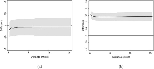The null hypothesis $H_0^3$: $NI\left({\mathcal{F}}_0,d\right)=NI\left({\mathcal{F}}_1,d\right)$ for at least some $d$ is clearly rejected in favour of a dominance alternative, as shown in Figure 2(b).

Figure 2. Neighbourhood inequality in Chicago, IL, 2014, versus two counterfactual distributions.

Note: Author analysis of US Census and American Community Survey (ACS) data. Confidence intervals are at the 95% level. (a) NI(F₀, d) - NI(F₁, d), (b) NI(F₀, d) - NI(F², d).

The simulation study is based on models for the income process $Y_f^n\sim \left({\mu }_f,{\sigma }_f^2,{\gamma }_f(.)\right)$ that is normal distributed with finite moments estimated on ${\mathcal{F}}_f$ with $f=0,1,2$. The Monte Carlo experiment consists in randomly drawing realizations from $Y_f^n$, each denoted $y_{f,r}^n$ with $r=1,\dots ,200$, and assessing relevant nulls hypothesis at predetermined distance threshold and for variable $n$. For samples of size $n=2000,5000,8000$, distance cut-offs are set at approximately one-third of a mile distance range increments within the first 2 miles, and then at increasing increments within the next 12 miles (at 19 miles’ range the NI index converges to citywide inequality). For the sample of size $n=1000$, distance thresholds within 1 and 19 miles are set by looking at increments of 0.75 mile exclusively. $H_0^3\left(d\right)$ is tested at each distance cut-off. The null hypothesis of the type $H_0^3$ is tested instead by looking at all distance cut-offs. For a detailed description of the Monte Carlo study, see Appendix in the supplemental data online.

We first investigate the size for the tests for various null hypothesis about NI curves. The size corresponds to the fraction of simulated samples that allow to reject the relevant null hypothesis when the null hypothesis is true in the population. We consider populations where $H_0^3$: $NI\left({\mathcal{F}}_0,d\right)=NI\left({\mathcal{F}}_1,d\right)$ for at least some $d$ is true. We draw replicas $y_{0,r}^n$ and $y_{1,r}^n$, and we test whether $H_0^3\left(d\right)$:$NI\left(y_{0,r}^n,d\right)=NI\left(y_{1,r}^n,d\right)$, as well as the implied null $H_0^3$, are rejected by the data. Rejections are recorded and the average share of rejections over the 200 replicas is stored in Table 1(A). Columns (1) to (9) report the size of test for null hypothesis $H_0^3\left(d\right)$ at well-defined distance cut-offs. Column (10) reports the average number of rejections of $H_0^3\left(d\right)$ across all available distance cut-offs. Column (11) reports the proportion of times that a null hypothesis $H_0^3\left(d\right)$ is rejected at least one. Columns (12) and (13) report, respectively, the share of cases where the rejection entails a weak dominance in NI curves (i.e., all cases where multiple rejections of $H_0^3\left(d\right)$ occur within the same replica $r$ and differences in NI curves have the same sign) and the proportion of the cases in (12) where dominance is strong (i.e., $H_0^3$ is rejected at every distance cut-off).

Table 1. Monte Carlo simulations of the size and power of dominance tests for NI curves that are based on the NI index SE approximations.

	Distance cut-offs (miles)									# Rejected	Rejected	Weak	Strong
	0.4	0.7	1	1.4	1.7	2	3	5	12
$n$	(1)	(2)	(3)	(4)	(5)	(6)	(7)	(8)	(9)	(10)	(11)	(12)	(13)
(A) Size comparisons for the true null $H_0^3:NI(y_{0,r}^n,d)=NI(y_{1,r}^n,d),\mathrm{\forall }d$
1000	.	0.00	.	0.24	.	0.19	0.16	0.03	0.01	1.1	0.46	0.60	0.00
2000	0.00	0.00	0.32	0.22	0.23	0.19	0.10	0.08	0.00	2.4	0.62	0.53	0.00
5000	0.00	0.00	0.33	0.15	0.17	0.09	0.01	0.01	0.00	1.1	0.52	0.47	0.00
8000	0.00	0.00	0.22	0.06	0.09	0.06	0.05	0.01	0.00	0.8	0.38	0.53	0.00
(B) Power comparisons for the true alternative $H_a^3:NI(y_{0,r}^n,d)\ge NI(y_{2,r}^n,d),\mathrm{\forall }d$
1000	.	0.00	.	0.29	.	0.31	0.19	0.09	0.03	1.7	0.60	0.92	0.00
2000	0.00	0.00	0.40	0.31	0.44	0.26	0.13	0.08	0.00	3.3	0.85	0.88	0.00
5000	0.00	0.00	0.55	0.28	0.49	0.24	0.12	0.09	0.03	4.3	0.81	0.98	0.00
8000	0.00	0.05	0.57	0.34	0.53	0.32	0.30	0.22	0.15	8.7	0.82	0.99	0.00

Overall, the tests based on the NI index SE bounds have larger size compared with the nominal 5% level. The size of tests carried out at fixed distance cut-offs is < 10% when the sample size is at least of 5000 units and it is virtually zero when $d\le 1$ mile. Tests for $H_0^3\left(d\right)$ for $d\ge 5$ miles are < 5%. At these distance ranges, in fact, neighbourhood inequality converges to the levels of citywide inequality measured by the Gini coefficient, and the SE approximation converges asymptotically (since the spatial association of incomes becomes negligible). On average, there is fewer than one rejection of $H_0^3\left(d\right)$ across the distance cut-offs for which we test. The upper bound for the size is of 18% in the largest sample. The size of the test monotonically converges to this number as the sample size grows. A linear interpolation of size estimates in column (11) suggests that the upper bound for the size converges to its nominal value of 5% when the sample size is > 16,000 units.

We also investigate the power of the tests for various null hypothesis about NI curves. Power is measured by the share of replicas that reject the relevant null hypothesis in favour of a specific alternative when the alternative is true in the population. We use distributions so that $H_0^3$: $NI\left({\mathcal{F}}_0,d\right)=NI\left({\mathcal{F}}_2,d\right)$ for at least some $d$ is rejected in favour of (strong) dominance in NI curves. We draw replicas $y_{0,r}^n$ and $y_{2,r}^n$ and we test if $H_0^3\left(d\right)$: $NI\left(y_{0,r}^n,d\right)=NI\left(y_{2,r}^n,d\right)$ at each distance cut-off separately, as well as the implied null $H_0^3$, are rejected by the data. We find that the power of tests for $H_0^3\left(d\right)$ are relatively small for small and large distance cut-offs, while power grows > 30% for distance cut-offs between 1 and 5 miles for which we test. Tests for $H_0^3$ neglect the positive correlation between SE computed at different distance cut-offs, thus making rejections of the null hypothesis more likely (since part of the variability in NI curves estimates is neglected). Hence, rejections rates for $H_0^3$ in favour of (weak) dominance can only be interpreted as upper bounds for the power of the joint tests. These upper bounds are estimated by the product of the columns (11) and (12). The upper bound for the power of tests for $H_0^3$ is of 74.8% for samples of size 2000 units and grows to 81% in the largest samples. Despite being upper bounds, these power estimates support the validity of tests for NI curves dominance based on the SE approximations even in relatively small samples. We also find that the average number of distance cut-offs where $H_0^3\left(d\right)$ is rejected at any given simulated sample grows steadily with the simulated sample size (column (10)), from 1.7 rejections when $n=1000$ to 8.7 rejections on average when $n=8000$, alongside larger chances that these rejections are in favour of a weak form of dominance in NI curves. Altogether, these figures confirm the relevance of the SE approximations for inferring about patterns and dynamics of neighbourhood inequality.

Additional checks

In Appendix C in the supplemental data online, we challenge the normality assumption. First, we derive SE bounds for the NI index while assuming stationarity and log-normality of the process as a reasonable alternative. Estimated bounds are marginally larger than those obtained under normality, implying a smaller rejection region. In the Monte Carlo experiment, we maintain the assumption that SE bounds are derived under normality and apply these bounds to simulated data from counterfactual joint log-normal (hence, non-gaussian) distributions. Compared with the results in Table 1, the simulated size seems not affected by lack of normality in the underlying data, while we register improvements in simulated power estimates. This may follow from the larger acceptance region implied by the normality assumption. Overall, evidence suggests that the normality assumption leads to high-power and high-conservative tests for the null of lack of changes in neighbourhood inequality.

Appendix D in the supplemental data online also considers the implications of edge effects arising from the choice of boundaries of the urban areas. A simulation exercise aims at assessing the implications of such effects by considering the spatial income distributions of Chicago, 2014, alongside a buffer zone on the boundaries: inequality measured in the individual neighbourhoods of those living in the buffer area does not contribute to NI computation (Griffith, 1983; Xu & Dowd, 2012). The sizes of the tests based on the simulated distributions (under normality) are comparable with those in Table 1, but smaller for samples of 8000 units. Accounting for edge effects reduces the power of the tests for $H_0^3$, although the difference with Table 1 is mitigated when rising sample size.

INFERENCE FOR PATTERNS AND TRENDS OF NEIGHBOURHOOD INEQUALITY IN CHICAGO, IL, 1980–2014

Andreoli and Peluso (2018) provide robust evidence that neighbourhood inequality is high in large American metro areas, it has been growing over the last 35 years, and it almost converges to citywide income inequality, even when estimates are based on individual neighbourhoods of small size (< 0.5 mile). Are these patterns producing reliable evidence for the population? Is the growth in neighbourhood inequality statistically significant?

We use the data for the metropolitan statistical area of Chicago in 1980, 1990, 2000 and 2014 to infer about dominance in NI curves.⁷ Chicago has experienced large demographic growth over the last 35 years, with the number of inhabited census blocks (each gathering approximately 1000 households) increasing from 3756 in 1980 to more than 4700 in 2014. The growth in average equivalent income (in nominal terms), ranging from US$13,794 in 1980 to US$55,710 in 2014, has been followed by an expansion of relative inequality. The Gini index for the citywide income distribution has evolved steadily, from 0.434 in 1980 to 0.461 in 1990, then to 0.473 in 2000, and finally to 0.486 in 2014, reflecting both demographic and economic changes.

Neighbourhood inequality in Chicago mirrors the trends observed in other large American metro areas. As shown in Figure 3(a), in each year the NI index is high and close to the level of the citywide Gini index even in neighbourhoods of relatively small size.⁸ The NI estimates are always significant at all distance ranges, with SE of the magnitude of $0.01-0.02$ points. As Table 2(A) shows, hypothesis $H_0^1$ is rejected with p-values always close to zero when the individual neighbourhood size is < 5 miles. When the individual neighbourhood is of ≥12 miles, neighbourhood inequality is statistically indistinguishable from the level of inequality observed in the city at conventional levels of significance in 1980, 2000 and 2014. Table 2(B) reports the evolution of the NI index at different distance thresholds compared with the level of neighbourhood inequality in individual neighbourhoods of size 0.4 miles. The gap in the NI index, in italics, is positive almost everywhere and always increasing with distance. Nonetheless, these differences are not statistically significant in a distance range < 5 miles. At 12 miles, $H_0^2$ can be rejected in every year with p-values that are slightly > 5% (smaller in 1990). The patterns of p-values confirm the findings of Andreoli and Peluso (2018) that after the year 2000 the degree of neighbourhood inequality registered in small neighbourhoods has become more representative of the degree of inequality in the city.

Figure 3. Trends in neighbourhood inequality in Chicago, IL.

Note: Author analysis of US Census and American Community Survey (ACS) data. Confidence intervals are at the 95% level.

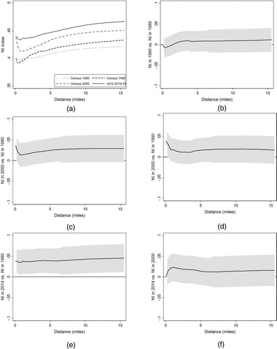
Table 2. P-values for the null hypothesis of the type $H_0^1:NI\left(y_t,d\right)=G\left(y_t\right)$ and $H_0^2:NI\left(y_t,d\right)=NI\left(y_t,0.4\right)$, with $t=1980,1990,2000,2014$ and $G\left(y_{1980}\right)=0.434$, $G\left(y_{1990}\right)=0.461$, $G\left(y_{2000}\right)=0.473$, $G\left(y_{2014}\right)=0.486$.

Years	Distance $d$ (miles)
2–7	0.4	1	2	3	5	12
(A) p-values for $H_0^1$
1980	0.000	0.000	0.000	0.000	0.004	0.160
1990	0.000	0.000	0.000	0.000	0.000	0.003
2000	0.000	0.000	0.000	0.000	0.001	0.070
2014	0.000	0.000	0.000	0.000	0.002	0.108
(B) p-values for $H_0^2$
1980	.	0.493	0.454	0.396	0.239	0.067
	0	0.000	0.001	0.003	0.009	0.020
1990	.	0.357	0.122	0.046	0.020	0.002
	0	0.004	0.014	0.020	0.025	0.039
2000	.	0.311	0.410	0.461	0.239	0.060
	0	−0.008	−0.004	0.002	0.012	0.027
2014	.	0.467	0.465	0.390	0.269	0.071
	0	−0.001	0.002	0.005	0.011	0.027

Note: Differences in levels of the neighborhood inequality (NI) index are shown in italics.

The trends of neighbourhood inequality in Chicago resemble those observed in other large American metro areas. The year-to-year changes in NI, reported in panels (b), (c) and (d) of Figure 3, are always positive at every distance range. The magnitude of these changes is, however, too small to be statistically significant according to the rejection region implied by the SE bounds. Nonetheless, the cumulated change of neighbourhood inequality over the four decades turns out to be positive and significant at every distance range. As panel (f) of Figure 3 shows, the acceptance region for $H_0^3$ is always positive and never includes the horizontal axis, implying that we have strong statistical evidence that the NI curve of Chicago for 2014 lies always above that of 1980 and the gap between these two curves is different from (in fact, larger than) zero.

CONCLUSIONS

This paper provides variance bounds for the neighbourhood inequality index. These bounds are identified from the knowledge of the variogram function which, under assumptions on the income-generating process that are common in spatial statistics literature, fully characterizes the spatial income distribution.

An application to rich income data from the US Census and ACS motivates the interest in using SE approximations for the NI index when assessing patterns and trends of neighbourhood inequality across US cities. Focusing on the city of Chicago, IL, we find robust statistical evidence that neighbourhood inequality is large even for individual neighbourhoods of small size, but it is statistically different from citywide inequality (as measured by the Gini index). The cumulated growth of neighbourhood inequality over the period 1980–2014 is substantial and significant at standard confidence levels, reflecting a general trend in largest American cities documented by Andreoli and Peluso (2018). Patterns are robust to granularity of the spatial distribution as well as to edge effects. The Monte Carlo study reveals that the tests for NI curves dominance based on the SE approximations have a higher size than the nominal values, although the (upper bound) size estimates quickly converge when the sample size grows. We expect that a sample of 16,000 units, smaller than the sample used to obtain estimates on the five-year ACS module, is sufficient to guarantee that the size of the tests we consider converge to their nominal values. The power of these tests is relatively small for null hypotheses defined at given distance cut-offs (but > 30% in simulated samples of at least 8000 units), but power grows significantly to > 80% when considering tests for NI curves (weak) dominance (although these are only upper bounds). Investigations about the appropriate testing procedure when placing dominance/non-dominance of NI curves under the null are also left for future research.

An interesting extension is to design individual neighbourhoods based on a nearest-neighbour logic, that is, by holding $n_{d_i}$ as fixed and $d$ variable. Cressie (1991) provides estimators for the variogram based on nearest-neighbour logic. While the nearest-neighbourhood weighting scheme bears little practical implications for calculating spatial statistics like the NI index at small geographical scale (LeSage & Pace, 2014), it fails basic replication invariance properties. Consider, for instance, the possibility of ‘replicating’ the population so that each income unit’s replica has the same income and location as the original. This operation doubles the population size and density of a city, without affecting the patterns of spatial income inequality. The NI index we study in this paper, which is normalized by population density, is not affected by this transformation. Conversely, a measure of neighbourhood inequality based on the nearest-neighbourhood logic would artificially dilute inequality evaluations over a larger number of neighbours. These arguments provide further support for the use of a distance-based criteria, such as the individual neighbourhood, in spatial inequality measurement.

ACKNOWLEDGEMENT

The authors are grateful to Flavio Santi, three anonymous referees and the editor for their valuable comments. Any errors are, of course, the authors’ alone. For the replication code, see Francesco Andreoli’s https://iris.univr.it/handle/11562/1021169“ \l ”.X3-Y4WgzZdh.

DISCLOSURE STATEMENT

No potential conflict of interest was reported by the author(s).

Additional information

Funding

This paper forms part of the research project The Measurement of Ordinal and Multidimensional Inequalities [grant number ANR-16-CE41-0005-01] of the Agence Nationale de la Recherche (French National Research Agency) and the projects MOBILIFE [grant number RBVR17KFHX] and PREOPP [grant number RBVR19FSFA] of the Università degli Studi di Verona (University of Verona) Basic Research scheme, whose financial support is gratefully acknowledged.

Notes

1 Under second-order stationarity, the spatial autocorrelation is ${\rho }_d=c\left(d\right)/{\sigma }^2$, which implies $\gamma \left(d\right)={\sigma }^2\left(1-{\rho }_d\right)$. When data are i.i.d., $\gamma \left(d\right)={\sigma }^2$ and NI is a local measure of inequality. Otherwise, the NI index is capable of measuring the consequences of spatial autocorrelation in the data (likely displaying ${\rho }_d>0$) on local inequality estimates.

2 It can be showed that $E\left[\left|Y_s-Y_v\right|\right]=\sqrt{2Var\left[Y_s-Y_v\right]/\pi }=\sigma \sqrt{2/\pi }$ for any pair of i.i.d. normal random variables $Y_s,Y_v$. It follows from Muliere and Scarsini (1989) that the Gini index writes $\left(E\left[\left|Y_s-Y_v\right|\right]/E\left[Y_v\right]\right)=\sqrt{2/\pi }\left(\sigma /\mu \right)$, which is a scaled version of the coefficient of variation. In our setting, when $d$ is large, $\gamma \left(d\right)=\sigma$. If the spatial process is i.i.d., then $NI\left({\mathcal{F}}_{\mathcal{S}},d\right)$ coincides with the Gini index at any distance threshold $d$.

3 When $d$ is large enough to include multiple urban areas, the graph of NI plotted against $d$ may not flatten for $d$ large. The meaningfulness of this computation rests, however, on the interest in analysing individual neighbourhoods that span over multiple urban aggregates.

4 Bias can be attenuated by smoothing the observed distribution of locations using kernel estimators. As shown by Zimmerman (2008), large samples need substantially less smoothing across locations to reduce the bias, holding fixed the geographical size of the city, thus supporting the use of $n_{d_i}$.

5 The sample counterpart of the NI index in (4) can be interpreted as a U-statistic. As shown by Hoeffding (1948, theorem 7.5), the variance bound in (5) converges to the asymptotic unbiased estimator of the NI index variance when the income observations are i.i.d. Under this specific circumstance, asymptotic normality is also granted both with simple or with complex sampling design (Davidson, 2009; Xu, 2007).

6 $H_0^3$ cannot be rejected if there is evidence of at least some intersection between the curves. It is rejected if one curve lies everywhere above the other, implying that the former distribution displays more spatial inequality than the other irrespectively of the choice of the distance parameter. The suggested procedure of joint testing is analogous to that used in stochastic dominance analysis (Dardanoni & Forcina, 1999). One can test for intersections of cumulative distribution functions against the alternative of strong first order stochastic dominance by producing t-tests for the intersection of cumulative distribution functions at any given income percentile (usually a grid). The null is rejected when the smallest t-test value recorded across percentiles range is larger than the corresponding 95% percentile of a standardized normal distribution (see also Andreoli, 2018; Bishop et al., 1989). We use the same logic to test for equality in NI curves taking dominance as the alternative.

7 See Andreoli and Peluso (2018) for details about the data. We use equivalized household market income estimates as observations; each is assumed to be located at the block group’s centroid. This assumption follows the empirical constraints dictated by the way data are organized into small areal units (block groups), whereas the NI index is defined for spatially continuous processes. In a simulation exercise discussed in Appendix E in the supplemental data online, we test the robustness of our estimates to such assumption.

8 The nature of the census and ACS publicly accessible data does not allow us to estimate unbiasedly NI in neighbourhoods < 0.3 miles. Confidence intervals are only reported for larger neighbourhoods.

REFERENCES

- Andreoli, F. (2018). Robust inference for inverse stochastic dominance. Journal of Business & Economic Statistics, 36(1), 146–159. https://doi.org/10.1080/07350015.2015.1137758
- Andreoli, F., & Peluso, E. (2018). So close yet so unequal: Neighborhood inequality in American cities. ECINEQ Working paper 2018-477.
- Baum-Snow, N., & Pavan, R. (2013). Inequality and city size. The Review of Economics and Statistics, 95(5), 1535–1548. https://doi.org/10.1162/REST_a_00328
- Biondi, F., & Qeadan, F. (2008). Inequality in paleorecords. Ecology, 89(4), 1056–1067. https://doi.org/10.1890/07-0783.1
- Bishop, J. A., Chakraborti, S., & Thistle, P. D. (1989). Asymptotically distribution-free statistical inference for generalized Lorenz curves. The Review of Economics and Statistics, 71(4), 725–727. http://www.jstor.org/stable/1928121 https://doi.org/10.2307/1928121
- Chakravorty, S. (1996). A measurement of spatial disparity: The case of income inequality. Urban Studies, 33(9), 1671–1686. https://doi.org/10.1080/0042098966556
- Chetty, R., & Hendren, N. (2018). The impacts of neighborhoods on intergenerational mobility i: Childhood exposure effects. The Quarterly Journal of Economics, 133(3), 1107–1162. https://doi.org/10.1093/qje/qjy007
- Chetty, R., Stepner, M., Abraham, S., Lin, S., Scuderi, B., Turner, N., Bergeron, A., & Cutler, D. (2016). The association between income and life expectancy in the United States, 2001–2014. The Journal of the American Medical Association, 315(14), 1750–1766. https://doi.org/10.1001/jama.2016.4226
- Chilès, J.-P., & Delfiner, P. (2012). Geostatistics: Modeling spatial uncertainty. John Wiley & Sons.
- Clark, W. A. V., Anderson, E., Östh, J., & Malmberg, B. (2015). A multiscalar analysis of neighborhood composition in Los Angeles, 2000–2010: A location-based approach to segregation and diversity. Annals of the Association of American Geographers, 105(6), 1260–1284. https://doi.org/10.1080/00045608.2015.1072790
- Conley, T. G., & Topa, G. (2002). Socio-economic distance and spatial patterns in unemployment. Journal of Applied Econometrics, 17(4), 303–327. https://doi.org/10.1002/jae.670
- Cressie, N. (1985). Fitting variogram models by weighted least squares. Journal of the International Association for Mathematical Geology, 17(5), 563–586. https://doi.org/10.1007/BF01032109
- Cressie, N., & Hawkins, D. M. (1980). Robust estimation of the variogram: I. Journal of the International Association for Mathematical Geology, 12(2), 115–125. https://doi.org/10.1007/BF01035243
- Cressie, N. A. C. (1991). Statistics for spatial data. John Wiley & Sons.
- Dardanoni, V., & Forcina, A. (1999). Inference for Lorenz curve orderings. The Econometrics Journal, 2(1), 49–75. https://doi.org/10.1111/1368-423X.00020
- Davidson, R. (2009). Reliable inference for the Gini index. Journal of Econometrics, 150(1), 30–40. http://www.sciencedirect.com/science/article/pii/S0304407609000323 https://doi.org/10.1016/j.jeconom.2008.11.004
- Dawkins, C. J. (2007). Space and the measurement of income segregation. Journal of Regional Science, 47(2), 255–272. https://doi.org/10.1111/j.1467-9787.2007.00508.x
- Diggle, P. (1985). A kernel method for smoothing point process data. Journal of the Royal Statistical Society. Series C (Applied Statistics), 34(2), 138–147. https://doi.org/10.2307/2347366.
- Doran, J., Jordan, D., & Elhorst, P. (2018). Virtual special issue on regional inequality. Spatial Economic Analysis, 13(4), 383–386. https://doi.org/10.1080/17421772.2018.1514095
- Echenique, F., & Fryer, R. G. (2007). A measure of segregation based on social interactions. The Quarterly Journal of Economics, 122(2), 441–485. https://doi.org/10.1162/qjec.122.2.441
- Galster, G. (2001). On the nature of neighbourhood. Urban Studies, 38(12), 2111–2124. http://usj.sagepub.com/content/38/12/2111.abstract https://doi.org/10.1080/00420980120087072
- Goodman, L. A., & Hartley, H. O. (1958). The precision of unbiased ratio-type estimators. Journal of the American Statistical Association, 53(282), 491–508. http://www.jstor.org/stable/2281870 https://doi.org/10.1080/01621459.1958.10501454
- Griffith, D. A. (1983). The boundary value problem in spatial statistical analysis. Journal of Regional Science, 23(3), 377–387. https://onlinelibrary.wiley.com/doi/abs/10.1111/j.1467-9787.1983.tb00996.x https://doi.org/10.1111/j.1467-9787.1983.tb00996.x
- Hardman, A., & Ioannides, Y. (2004). Neighbors’ income distribution: Economic segregation and mixing in US urban neighborhoods. Journal of Housing Economics, 13(4), 368–382. https://doi.org/10.1016/j.jhe.2004.09.003
- Hoeffding, W. (1948). A class of statistics with asymptotically normal distribution. The Annals of Mathematical Statistics, 19(3), 293–325. http://www.jstor.org/stable/2235637 https://doi.org/10.1214/aoms/1177730196
- Iceland, J., & Hernandez, E. (2017). Understanding trends in concentrated poverty: 1980–2014. Social Science Research, 62, 75–95. http://www.sciencedirect.com/science/article/pii/S0049089X1630059X https://doi.org/10.1016/j.ssresearch.2016.09.001
- Jargowsky, P. A. (1997). Poverty and place: Ghettos, barrios, and the American city. Russell Sage Foundation.
- Journel, A. G., & Huijbregts, C. J. (1989). Mining geostatistics. Academic Press.
- Kelejian, H. H., & Prucha, I. R. (2010). Specification and estimation of spatial autoregressive models with autoregressive and heteroskedastic disturbances. Journal of Econometrics, 157(1), 53–67. Nonlinear and Nonparametric Methods in Econometrics. http://www.sciencedirect.com/science/article/pii/S0304407609002784 https://doi.org/10.1016/j.jeconom.2009.10.025
- Kim, J., & Jargowsky, P. A. (2009). The Gini-coefficient and segregation on a continuous variable, Vol. Occupational and Residential Segregation of Research on Economic Inequality. Emerald Group Publishing Limited, pp. 57–70.
- Koop, J. C. (1964). On an identity for the variance of a ratio of two random variables. Journal of the Royal Statistical Society. Series B (Methodological), 26(3), 484–486. http://www.jstor.org/stable/2984501 https://doi.org/10.1111/j.2517-6161.1964.tb00578.x
- Leone, F. C., Nelson, L. S. & Nottingham, R. B. (1961). The folded normal distribution. Technometrics, 3(4), 543–550. http://www.jstor.org/stable/1266560 https://doi.org/10.1080/00401706.1961.10489974
- LeSage, J. P., & Pace, R. K. (2014). The biggest myth in spatial econometrics. Econometrics, 2(4), 217–249. https://doi.org/10.3390/econometrics2040217
- Li, H., Calder, C. A., & Cressie, N. (2007). Beyond Moran’s i: Testing for spatial dependence based on the spatial autoregressive model. Geographical Analysis, 39(4), 357–375. https://onlinelibrary.wiley.com/doi/abs/10.1111/j.1538-4632.2007.00708.x https://doi.org/10.1111/j.1538-4632.2007.00708.x
- Ludwig, J., Duncan, G. J., Gennetian, L. A., Katz, L. F., Kessler, R. C., Kling, J. R., & Sanbonmatsu, L. (2012). Neighborhood effects on the long-term well-being of low-income adults. Science, 337(6101), 1505–1510. http://science.sciencemag.org/content/337/6101/1505 https://doi.org/10.1126/science.1224648
- Ludwig, J., Duncan, G. J., Gennetian, L. A., Katz, L. F., Kessler, R. C., Kling, J. R., & Sanbonmatsu, L. (2013). Long-term neighborhood effects on low-income families: Evidence from Moving to Opportunity. American Economic Review, 103(3), 226–231. http://www.aeaweb.org/articles.php?doi=10.1257/aer.103.3.226 https://doi.org/10.1257/aer.103.3.226
- Ludwig, J., Sanbonmatsu, L., Gennetian, L., Adam, E., Duncan, G. J., Katz, L. F., Kessler, R. C., Kling, J. R., Lindau, S. T., Whitaker, R. C., & McDade, T. W. (2011). Neighborhoods, obesity, and diabetes – A randomized social experiment. New England Journal of Medicine, 365(16), 1509–1519. PMID: 22010917. https://doi.org/10.1056/NEJMsa1103216
- Massey, D. S., & Eggers, M. L. (1990). The ecology of inequality: Minorities and the concentration of poverty, 1970–1980. American Journal of Sociology, 95(5), 1153–1188. https://doi.org/10.1086/229425
- Matheron, G. (1963). Principles of geostatistics. Economic Geology, 58(8), 1246–1266. https://doi.org/10.2113/gsecongeo.58.8.1246
- Moretti, E. (2013). Real wage inequality. American Economic Journal: Applied Economics, 5(1), 65–103. http://www.aeaweb.org/articles?id=10.1257/app.5.1.65 https://doi.org/10.1257/app.5.1.65
- Muliere, P., & Scarsini, M. (1989). A note on stochastic dominance and inequality measures. Journal of Economic Theory, 49(2), 314–323. http://www.sciencedirect.com/science/article/pii/0022053189900847 https://doi.org/10.1016/0022-0531(89)90084-7
- Openshaw, S. (1983). The modifiable areal unit problem. Geo Books.
- Pyatt, G. (1976). On the interpretation and disaggregation of Gini coefficients. The Economic Journal, 86(342), 243–255. https://doi.org/10.2307/2230745
- Reardon, S. F., & Bischoff, K. (2011). Income inequality and income segregation. American Journal of Sociology, 116(4), 1092–1153. http://www.jstor.org/stable/10.1086/657114 https://doi.org/10.1086/657114
- Shorrocks, A., & Wan, G. (2005). Spatial decomposition of inequality. Journal of Economic Geography, 5(1), 59–81. https://doi.org/10.1093/jnlecg/lbh054
- Tin, M. (1965). Comparison of some ratio estimators. Journal of the American Statistical Association, 60(309), 294–307. http://www.jstor.org/stable/2283154 https://doi.org/10.1080/01621459.1965.10480792
- Watson, T. (2009). Inequality and the measurement of residential segregation by income in American neighborhoods. Review of Income and Wealth, 55(3), 820–844. https://onlinelibrary.wiley.com/doi/abs/10.1111/j.1475-4991.2009.00346.x https://doi.org/10.1111/j.1475-4991.2009.00346.x
- Wheeler, C. H., & La Jeunesse, E. A. (2008). Trends in neighborhood income inequality in the U.S.: 1980–2000. Journal of Regional Science, 48(5), 879–891. https://doi.org/10.1111/j.1467-9787.2008.00590.x
- Wong, D. (2009). The modifiable areal unit problem (MAUP). In A. S. Fotheringham & P. Rogerson (eds.). The SAGE handbook of spatial analysis (pp. 105-124). Los Angeles: Sage.
- Xu, C., & Dowd, P. A. (2012). The edge effect in Geostatistical simulations. Springer Netherlands. 115–127. https://doi.org/10.1007/978-94-007-4153-9˙10
- Xu, K. (2007). U-statistics and their asymptotic results for some inequality and poverty measures. Econometric Reviews, 26(5), 567–577. https://doi.org/10.1080/07474930701512170
- Zimmerman, D. L. (2008). Estimating the intensity of a spatial point process from locations coarsened by incomplete geocoding. Biometrics, 64(1), 262–270. http://www.jstor.org/stable/25502044 https://doi.org/10.1111/j.1541-0420.2007.00870.x