Store sales evaluation and prediction using spatial panel data models of sales components

ABSTRACT

This paper sets out a general framework for store sales evaluation and prediction. The sales of a retail chain with multiple stores are first decomposed into five components, and then each component is explained by store, competitor and consumer characteristics using random effects models for components observable at the store level and spatial error random effects models for components observable at the zip code level. We use spatial panel data over four years for estimation and a subsequent year for evaluating one-year-ahead predictions. Set against a benchmark model that explains total sales directly, the prediction error of our framework is reduced by 34% for existing stores during the sample period, by 5% for existing stores one year ahead and by 26% for new stores.

KEYWORDS:

• retailing
• decomposition
• sales components
• loyalty programmes
• spatial econometrics

JEL:

• C33
• C53
• M31

INTRODUCTION

Location remains a crucial driver of store performance in modern retail environments (Bell, 2014; Jank & Kannan, 2005; Levy & Weitz, 2004; Pan & Zinkhan, 2006). From a consumer perspective, travel distance to the store strongly affects its attractiveness, and from a retailer perspective, store location decisions involve massive and almost irreversible capital investments that largely determine the trade area of the store (Ailawadi & Keller, 2004; Briesch et al., 2009). Therefore, successful retailers routinely evaluate the performance of their current stores and predict the performance implications of potential location changes or new store openings (Gauri et al., 2009; Kumar & Karande, 2000).

These observations have given rise to quantitative approaches to decision-making about store locations (Buckner, 1998). Early models explaining and predicting store performance are commonly based on aggregated data. However, two recent developments offer new opportunities for store location research. First, the widespread availability of customer loyalty cards (Leenheer & Bijmolt, 2008) offers the opportunity to decompose total revenues of each individual store into different sales components (Van Heerde & Bijmolt, 2005), and to explain these components at a lower level of scale than its whole trade area. More specifically, loyalty card data offer the opportunity to compute how frequently a member visits the store and how much is spent each visit. By modelling these sales components separately, instead of just total sales, it becomes possible to test whether the drivers of store sales have different impacts on these components. Moreover, whereas traditional approaches assume that trade areas are homogeneous, that is, neighbourhoods have similar characteristics and spending patterns, the analysis of customer data and the collection of additional aggregate consumer characteristics from census data at the zip code level offers the opportunity to link local differences in shopping behaviour to local differences in consumer characteristics (Steenburgh et al., 2003).

Second, the use of data at a lower level of scale provides a means to better predict individual sales components by borrowing relevant information from neighbouring locations. Smaller units in close proximity to one another often share the same unobserved characteristics, such as sociodemographic factors, economic circumstances, and local road and public transport networks, as a result of which they cannot be treated as independent entities (Anselin, 1988; LeSage & Pace, 2009). For this reason, we account for spatial error dependence and evaluate to which extent it improves predictive performance. Spatial econometric models gain more and more attention in the marketing literature (for overviews, see Bradlow et al., 2005: Bronnenberg, 2005; Elhorst, 2017; and Hartmann et al., 2008). However, a relatively unexplored issue is the extent to which spatial econometric models can also be used for prediction purposes. The spatial econometric literature on prediction can be subdivided into two parts. One part that focuses on spatial panel data and develops formulas for out-of-sample predictions for in-sample observations in the future (Baltagi & Li, 2004, 2006; Baltagi et al., 2012; Elhorst, 2005; Fingleton, 2009), and another part that employs in-sample units of observations to predict out-of-sample units in a cross-sectional setting (Goulard et al., 2017; Kato, 2008; Kelejian & Prucha, 2007). This paper employs insights from the first part to predict sales components of existing stores during the sample period and one year ahead, and insights from the second part to predict sales components of new stores. Baltagi et al. (2012) state that the literature on forecasting observations based on spatial panels is still scarce. This holds especially for empirical applications focusing on firm and store performance, and applications that decompose their sales into different components.

We exploit these two developments by proposing and testing an advanced framework for store sales prediction. This framework decomposes total sales into different sales components at both the store and zip code levels, and accounts for random effects when explaining sales components observed at the store level and for both random effects and spatial dependence when explaining sales components observed at the zip code level. It is shown that this framework leads to better sales predictions for both existing and new stores. The wider implication of this finding is that the proposed framework is a useful tool for (1) evaluating the performance of existing stores, (2) predicting the future performance of existing stores and (3) predicting the sales of possible new stores. In addition, if sales levels fall below expected levels, the decomposition approach also informs store managers which sales components are responsible for this and need improvement. Hence, by using and also partly further developing the latest spatial econometric techniques, we advance the currently available models for explaining store sales and offer store managers more detailed insights about the performance of store sales components than a model just explains store total sales directly.

The remainder of the paper is structured as follows. In the next section we provide a brief overview of existing store location evaluation models in the marketing literature that serves as a starting point for further model development. In the third section we set out the decomposition framework for modelling store sales in line with the data obtained from a Dutch retail clothing chain which are discussed in the fourth section. In the fifth section we present the econometric models that we use to explain the store sales components obtained from our decomposition framework, and the corresponding prediction equations. In the sixth section we report and discuss the empirical results. In the seventh section we evaluate the predictive power of our proposed model relative to a benchmark model that explains total sales directly. We also provide managerial implications of how the retailer can identify areas that are under- or overperforming. Finally, we draw conclusions in the eighth section.

LITERATURE REVIEW

Various analytical tools attempt to evaluate store location decisions (Buckner, 1998; Levy & Weitz, 2004), mostly by considering the amount of sales each location can generate in a certain period, given the current spatial distribution of demand and competition. Huff’s gravity model and its extensions provide one of the earliest applications of spatial models in marketing, but they are still used today. For example, Del Gatto and Mastinu (2018) empirically examine whether Italian retailers satisfy the Huff model. These models predict the geographical extent of store trade areas on the basis of a negative relation between store patronage and distance to consumers. They explain the proportion of visits from a certain area to the store, but not any changes in consumers’ expenditures. To predict sales, the probability that a consumer will visit the store from a particular location is multiplied by an estimate of the (average) expenditures at that location and by population size or, alternatively, by (average) expenditures per household and number of households. Generally, these models do not include consumer and store characteristics other than store size; they assume that store patronage depends only on store size and distance to the store.

Regression models enable analysts to identify several factors associated with different levels of sales from stores at different sites. However, existing studies use aggregate measures of consumer demographics for the entire trade area to predict sales at a particular store location, even though retailers in most Western countries serve trade areas with a rather heterogeneous population (Campo & Gijsbrechts, 2004; Singh et al., 2006). Other studies reveal that the geographical location of consumers and their demographics can be an important variable for predicting consumer behaviour (Yang & Allenby, 2003). Within the spatial economics literature, De Mello-Sampayo (2016) explains which services patients use in the case of healthcare when these services are spread over different locations, while Öner (2017) determines whether consumers’ access to retail units in Sweden is relevant for the attractiveness of municipalities.

In addition, a growing literature on spatial models in marketing (see Elhorst, 2017, for a recent overview) reveals how spatial covariation in sales can be exploited to gain better insights into the effectiveness of marketing activities across markets. Yet, these spatial effects heretofore have been mostly ignored in the store location literature (Duan & Mela, 2009). Many studies also consider sales in general (Kumar & Karande, 2000) and offer no insights in the underlying mechanisms causing changes in store sales components. Pan and Zinkhan (2006), however, demonstrate that various regressors can have different effects across sales components, which suggests that decomposing sales (effects) into constituent parts may offer richer insights than a model of total store sales only. Furthermore, if store managers want to understand why sales levels are lagging and act accordingly, they will benefit from knowing which sales components need improvement to achieve the desired sales levels.

Another stream of research (Chan et al., 2007; Chintagunta et al., 2006; Duan & Mela, 2009; Thomadsen, 2007) determines equilibrium prices or sales conditional on outlet location and capacity. These studies show that location competition affects sales, positively or negatively, while the reverse can be true as well; that is, (potential) sales may attract competitors. To separate these alternative explanations, we not only employ the number of competitors as an explanatory variable of store sales components, but also include an equation explaining the number of competitors at a particular location.

STORE REVENUES DECOMPOSITION

We propose a decomposition framework for evaluating current and future store performance of a retailer with access to customer data through a loyalty programme. The decompositions are illustrated in Figure 1 in reverse order to that discussed below.

Figure 1. Decomposition framework for store sales.

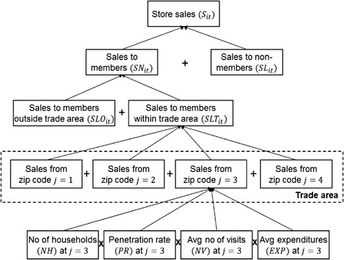
If a loyalty programme member makes a purchase at one of the stores of the focal chain, this transaction is automatically registered and attributed to the loyalty member’s account. From the retail chain’s perspective, loyalty card data provide detailed information about the shopping behaviour of each member, among which how frequently a member visits the store and how much is spent each visit. Customers who sign up for loyalty programmes also provide the retailer with their addresses, which can be used to allocate revenues to the zip codes in which the members are living.

These features of loyalty programmes enable us to measure the membership rate, visit frequency and average amount spent per visit for each zip code, because revenues to loyalty programme members in zip code $j$ at time $t$ can be decomposed as follows: (1) $S{L}_{jt}\equiv N{H}_{jt}\times P{R}_{jt}\times N{V}_{jt}\times EX{P}_{jt},$(1) where the index j refers to zip codes ($j=1,\cdots ,J$), and t to a given time period ($t=1,\cdots ,T$); SL is sales to members; NH is the number of households; PR is the penetration rate of the loyalty card (the share of members in a zip code); NV is the average number of visits of members; and EXP is the average expenditures per visit of members. This distinction of sales to members into four components observable at the zip code level is represented by the bottom decomposition in Figure 1. By modelling these sales components separately, instead of just total sales, it becomes possible to test whether the determinants of store sales have different impacts on these components.

Despite the focus on loyalty programme members, not all loyalty programme members are equally important for a retailer. We distinguish between those who live in a store’s trade area and those who live elsewhere. Knowledge about the store’s trade area is essential because it allows retailers to identify and serve the consumers who are most likely to purchase. Trade areas typically consist of two or three zones (Levy & Weitz, 2004), depending on the amount of sales generated in each area. A store’s primary trade area is the zone from which it gets most of its sales – usually about 65% of total sales. The secondary zone generates the next 20% of total sales, whereas the tertiary zone captures sales from non-regular visitors (i.e., the remaining 15–20%). Because we aim to model the purchase behaviour of regular visitors (read: loyalty card holders; Allaway et al., 2003; Van Heerde & Bijmolt, 2005), we focus on the primary and secondary zones and consider zip codes belonging to those two zones part of the store’s trade area. However, we also investigate the sensitivity of the results for considering 75% and 95% instead of 85% of total sales. This disaggregation of sales to members to different zip codes that are part of the trade area of each store is represented by the second bottom decomposition in Figure 1. Since these zip codes are linked to the trade area of a particular store, the sales components in equation (1) should also be indexed by store i ($i=1,\cdots ,I$), except for the number of households living in a zip code and the loyalty card penetration rate, since these are independent of a store:

$S{L}_{ijt}\equiv N{H}_{jt}\times P{R}_{jt}\times N{V}_{ijt}\times EX{P}_{ijt}$.

Decomposing store revenues into their substituent components at the zip code level addresses another important limitation of previous studies: the assumption that trade areas are homogeneous, while they typically consist of a mosaic of small zip codes with heterogeneous sociodemographic and lifestyle characteristics (Campo & Gijsbrechts, 2004). The viability of a store depends largely on its capability to satisfy the needs of consumers who live in the different parts of the trade area and to develop strategies to influence their responses to the store’s marketing activities (Campo & Gijsbrechts, 2004; Vroegrijk et al., 2016). A store can also adjust its profile depending on the demographic characteristics of its customer base. Therefore, store location evaluation models better determine the impact of (changes in) local trade area demographics on store sales. Census data can provide information about these characteristics. Because customers who sign up for loyalty programmes provide the retailer with their addresses, census data available at the lowest level of scale can be used to explain sales components observable at that level. Retailers often use the services of data intermediaries such as Claritas or Experian to augment their internal databases with descriptive information about customers. However, intermediaries cannot or are not allowed to provide data at an individual level because privacy laws require data intermediaries to ‘mask’ individual customer information by reporting it only at a geographically aggregate level. Hence, the data that we will use in this study are similar to the data that retailers tend to have at their disposal. The lowest level at which census data are available is the zip code level.

Total sales to loyalty programme members who live in the trade area of a store ($SL{T}_{it}$) are obtained by adding up the sales to members over all zip codes belonging to a store’s trade area ($S{L}_{ijt}$): (2) $SL{T}_{it}=\sum _{j=1}^{J_{it}}S{L}_{ijt},$(2) where $J_{it}$ is the number of zip codes belonging to the trade area of store i at time t. Total sales to all members of the chain $\left(S{L}_{it}\right)$ are subsequently obtained by adding up the sales to members living outside the trade area ($SL{O}_{it}$) to the sales to members living inside the trade area ($SL{T}_{it}$): (3) $S{L}_{it}=SL{O}_{it}+SL{T}_{it}.$(3) Finally, total sales of a store ($S_{it}$) are obtained by adding up sales to non-members ($S{N}_{it}$) and sales to members: (4) $S_{it}=S{L}_{it}+S{N}_{it}.$(4) The latter two distinctions between sales to members and non-members and between members within and outside the trade areas of stores are illustrated in Figure 1 by the first and the second decomposition of sales components.

In summary, we decompose sales ($S_{it}$) into six components: $S{N}_{it}$, $SL{O}_{it}$, $N{H}_{jt}$, $P{R}_{jt}$, $N{V}_{ijt}$ and $EX{P}_{ijt}$. Each component will be explained, except for the number of households living in a particular zip code, $N{H}_{jt}$, since this number may be treated as exogenous information to the retailer. To investigate whether this decomposition of total sales into different components is beneficial, we also consider a benchmark model that explains total sales ($S_{it}$) directly. Components indexed by j are explained at the zip code level, and without j at the store level.

DATA AND ADDITIONAL DEPENDENT VARIABLES

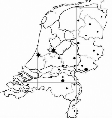
We use data from 28 clothing stores (26 existing stores and two new stores) that belong to a single chain in the Netherlands. The stores offer a medium-quality assortment and are mostly located in medium-sized towns. Figure 2 maps the locations of the existing and new stores. Since the retail chain has no stores in the western part yet, it is looking for potential new locations especially in this part of the country.

Figure 2. Existing (dots) and new (*) store locations of the retail chain.

Note: Dot sizes reflect store sizes.

We have data over a period of five years, of which we use the first four years for estimation and the last year for validation. The sample period of four years covers 102 observations (24 stores in the first and 26 stores in the next three years). Withholding the last year for validation enables us to verify one-year-ahead predictions for these existing stores. Since the chain opened two new stores in the last year, we can also assess to what extent our model results apply to these new stores.

The customer database contains personal data in addition to purchase data. We use the addresses of members to overlay several sociodemographic variables made available by WDM Nederland BV, part of the Swedish parent Bisnode. In addition, we supplement these data with information from a chain-wide survey among all 28 outlet managers that provides, for each store, information about the store itself and its competitive environment.

To determine the trade area of each store, we first sort all zip codes in descending order of travel distance to the nearest stores and then select, for each store and each year, the first sorted zip codes responsible for 85% of total sales (we also consider 75% and 95% of total sales). The perimeter of the trade area of a store is then defined as the travel distance of the last zip code that has been selected to the store. This travel distance is calculated as the fastest distance in miles a car can travel from (the centroid of) a four-digit zip code to the store under consideration. The number of zip codes belonging to a store’s trade area varies over time and across stores: from 44 to 307, with an average of 110 zip codes. Since this number of zip codes assigned to a store’s trade area depends on total sales, the perimeter of this trade area should be treated as an endogenous variable. This is important especially when using the model for prediction purposes. Total sales must then first be predicted before the trade area (perimeter) can be determined. We return to this below.

We explain the loyalty card penetration for all zip codes in the Netherlands (N = 4008) in four successive years, resulting in 16,032 (4008 zip codes × 4 years) observations. Since the trade areas of the stores mapped in Figure 2 do not cover the whole country, the number of observations of the number of visits amounts to 10,611 and on the expenditures per visit to 9726. The latter number is lower than the former because not every visitor also buys clothes. Although the average perimeter of a store’s trade area is 15.86 miles, its standard deviation of 5.54 indicates substantial variation in trade area sizes of the different stores. Almost 10% of the households within the trade areas has a loyalty card. On average, they visit the store 1.4 times a year and spend €67 per visit.

Following the extant literature, we employ store, consumer and competitor characteristics to explain store sales components, in addition to a constant and a time trend. For the store characteristics, we include store size, the relative size of the various departments (women’s, men’s and children’s assortments), the number of months the store is open in a particular year, and the number of years that has passed since the store was established.

In addition to store characteristics, many studies document possible relationships between consumer demographics and various components of store sales. Reinartz and Kumar (1999) find that the number of households living in the store’s trade area has the largest impact on store performance, followed by store attractiveness and socioeconomic status. The theory of time allocation between different activities, as used by Kumar and Karande (2000), suggests that store performance relies, among other things, on household income and size. Because high-income households have higher opportunity costs for their time, they tend to visit stores less frequently but spend more per visit. Pan and Zinkhan (2006) indicate that gender represents an important predictor of visit frequency, whereas store characteristics (e.g., service quality, store atmosphere) and product attributes (e.g., product selection, quality) determine store choice.

With respect to competitor characteristics, Singh et al. (2006) find that the entrance of a large competitor has a significant effect on the number of visits of loyalty programme members to an incumbent store, though the residence location of customers moderates this effect. Moreover, customer locations, as Allaway et al. (2003) show, influence a customer’s likelihood of adopting a new loyalty programme according to distance from the store. The number of nearby adopters at a particular location also influences the decision to join a new programme (Bell & Song, 2007). Thomadsen (2007) shows that locations with a large number of people matching the firm’s target customer profile typically attract a large number of competitors as well. Finally, Seim (2006) finds that undifferentiated firms avoid direct competition by locating their stores far from those of competitors.

These findings indicate that the number of competitors may not only be an important determinant of store sales components, but also that this variable might potentially be endogenous. For this reason, the number of competitors of a particular store is also explained in this study. We used information gathered from store managers to identify the number of (direct) competitors, who can be defined as clothing stores targeting the same customer segment. The number of competitors ranges from 22 to 78 across stores.

Detailed descriptive statistics (mean and standard deviation) of the dependent and independent variables used in this study, as well as their data sources, are reported in Tables 1 and 2. Table 1 covers variables measured at the store level and Table 2 those at the zip code level.

Table 1. Descriptive statistics of the store-level variables.

Dependent variable	Symbol	Mean	SD	Data source
% Non-members	$S{N}_{it}/S_{it}$	0.272	0.088	Sales register
% Outside trade area	$SL{O}_{it}/S{L}_{it}$	0.154	0.061	Sales register
Trade area perimeter	$TA{P}_{it}$	15.86	5.543	Public
Number of competitors	$N{C}_{it}$	42	12.642	Survey
Total sales	$S_{it}$	1.48 × 10^6	5.10 × 10^5	Sales register
Explanatory variables of dependent variables measured at the store level
Size (m^2)		713	110.626	Survey
Years since first established store		22.55	9.985	Survey
Proportion of year store is open		0.992	0.068	Survey
Population size (in 100,000)		0.801	0.402	Census
Nearest distance to other store (miles)		19.55	8.846	Public
Time trend		2.529	1.114	Authors’ own construction
% female assortment		0.439	0.050	Survey
% children’s assortment		0.202	0.049	Survey
% households with children		0.434	0.036	Census
% couples without children		0.388	0.022	Census
% households with high SES		0.213	0.014	Census
% households with above-average SES		0.078	0.024	Census
% households with average SES		0.316	0.029	Census
% households with low SES		0.427	0.039	Census
% of double-income families		0.139	0.021	Census
Average number of low educated		0.469	0.187	Census
> average number of low educated		0.338	0.100	Census
Average number of middle educated		0.100	0.063	Census
> average number of middle educated		0.775	0.078	Census
Average number of high educated		0.221	0.122	Census
> average number of high educated		0.307	0.080	Census
Average number of low educated		0.213	0.014	Census
> average number of low educated		0.078	0.024	Census

Table 2. Descriptive statistics of zip code-level variables.

Dependent variable	Symbol	Mean	SD				Data source
Loyalty card penetration rate	$P{R}_{jt}$	0.097	0.128				Sales register
Visits	$N{V}_{ijt}$	1.401	0.439				Sales register
Expenditures	$EX{P}_{ijt}$	67.326	29.897				Sales register

	$P{R}_{jt}$		$N{V}_{ijt}$		$EX{P}_{ijt}$
Explanatory variables of dependent variables measured at zip code level	Mean	SD	Mean	SD	Mean	SD
Size	771.210	285.534	746.255	107.493	745.296	109.239	Survey
% female assortment	0.421	0.045	0.428	0.043	0.430	0.044	Survey
% children’s assortment	0.202	0.043	0.199	0.044	0.199	0.045	Survey
Proportion of year store is open	0.993	0.064	0.996	0.050	0.995	0.053	Survey
Years since first established store	54.725	10.080	20.974	8.954	21.129	9.184	Survey
Number of competitors	39.770	11.121	44.322	13.132	45.007	13.057	Survey
Distance to the store	21.929	16.427	11.852	6.145	11.227	5.943	Public
Distance to next-nearest store	31.635	15.489	25.722	18.872	26.210	19.377	Public
% households with children	0.428	0.123	0.429	0.121	0.429	0.114	Census
% couples without children	0.382	0.094	0.389	0.087	0.389	0.079	Census
% households with high SES	0.080	0.126	0.083	0.126	0.079	0.111	Census
% households with above-average SES	0.315	0.203	0.321	0.190	0.320	0.177	Census
% households with average SES	0.417	0.211	0.421	0.198	0.424	0.184	Census
% households with low SES	0.138	0.135	0.135	0.129	0.137	0.121	Census
% of double-income families	0.213	0.057	0.213	0.053	0.213	0.049	Census
Average number of low educated	0.324	0.468	0.335	0.472	0.339	0.473	Census
> average number of low educated	0.469	0.499	0.461	0.499	0.474	0.499	Census
Average number of middle educated	0.744	0.436	0.758	0.428	0.782	0.413	Census
> average number of middle educated	0.104	0.305	0.097	0.296	0.095	0.294	Census
Average number of high educated	0.306	0.461	0.312	0.464	0.317	0.465	Census
> average number of high educated	0.241	0.427	0.245	0.430	0.217	0.412	Census
Time trend	2.500	1.118	2.538	1.114	2.527	1.114	Authors’ own construction

ECONOMETRIC MODEL SPECIFICATIONS AND PREDICTORS

In the previous two sections we derived eight store performance variables that need to be explained: five at the store level and three at the zip code level. In this section we will set out three different econometric models to explain these variables and three associated predictors. An overview of all the dependent variables, their description, the transformation applied to each variable, the type of model that will be used to explain them and the kind of predictors is provided in Table 3. The latter three items are explained below. We present the models and associated predictors in increasing degree of difficulty.

Table 3. Overview of dependent variables and type of model to explain and predict them.

Dependent variable	Description	Transformation	Econometric model^a	Predictor
S	Total sales	Log	Store-RE	Equation (6) + detransf.
TAP	Trade area perimeter	Log	Store-RE	Equation (6) + detransf.
SN/S	% non-member sales	Logit	Store-RE	Equation (6)
SLO/SL	% outside trade area sales	Logit	Store-RE	Equation (6)
NC	Number of competitors	Log	Store-RE	Equation (6) + detransf.
PR	Penetration rate	Logit	Zip-RE-SA	Equation (8)
NV	Number of visits	Log	Zip-Unbalanced-RE-SA	Equation (10) + detransf.
EXP	Expenditures	Log	Zip-Unbalanced-RE-SA	Equation (10) + detransf.

Note: ^aStore = explained at the store level; Zip = explained at the zip code level; RE = random effects; SA = spatial autocorrelation; Unbalanced = estimation and prediction based on unbalanced spatial panel data; Detransf. = detransformation correction from log to level based on Miller (1984).

The first model is used to explain dependent variables at the store level and in vector form reads as: (5) $Y_t=X_t\text{β}+v+{ϵ}_t$(5) where $Y_t$ denotes an $I\times 1$ vector consisting of one observation on the dependent variable for every store i at time t; and $X_t$ represents an $I\times K$ matrix of explanatory variables measured at the store level, among which the intercept and a time trend. The $K\times 1$ vector $\text{β}$ contains the corresponding response parameters of these explanatory variables. We further allow each store to have its own unobservable store-specific intercept $v_i$ with zero mean, $E\left(v_i\right)=0$, and constant variance, $Var\left(v_i\right)={\sigma }_v^2$. $v=(v_1,\cdots ,v_I{)}^{\mathrm{\prime }}$ stacks these random intercepts in vector form. This variable intercept controls for all time-invariant variables that are omitted from the model because they are difficult to measure or hard to obtain. Its random effects specification further assumes that the stores form a random draw from a larger population, which is in line with the aim of this paper that existing stores may be closed and new stores may be opened at other locations. Finally, ${ϵ}_t$ is a normally distributed error term with mean zero, $E\left({ϵ}_t\right)=0$, and constant variance, $Var\left({ϵ}_t\right)={\sigma }_{ϵ}^2{I}_I$. Since this model explains store-level variables and controls for random effects, we label it as the Store-RE model.

A detailed description how to obtain the maximum likelihood (ML) estimates of the parameters of the Store-RE model and their variance–covariance matrix is available in Elhorst (2014, section 3.2.2), building on previous work of Breusch (1987). Instead of ${\sigma }_v^2$ and ${\sigma }_{ϵ}^2$, ${\varphi }^2={\sigma }_{ϵ}^2/\left(T{\sigma }_v^2+{\sigma }_{ϵ}^2\right)$ and ${\sigma }_{ϵ}^2$ are estimated, where $0\le {\varphi }^2\le 1$ and $\varphi$ measures the weight to attach to the cross-sectional variation in the data, in addition to the time-series variation. In case $\varphi =1$, both types of variation are equally weighted, as a result of which the random effects estimator boils down to the ordinary least squares (OLS) estimator of the parameters of the model.

One of the most important elements of store location evaluation involves predicting sales. For each model in this section, we therefore also present the corresponding prediction formula. Baltagi and Li (2004, equation 13.14) show that the best linear unbiased predictor (BLUP) for the vector of all units in the sample at a future period t + h is given by: (6) ${\hat{Y}}_{t+h}=X_{t+h}\widehat{\text{β}}+{\displaystyle \frac{T{\sigma }_v^2}{T{\sigma }_v^2+{\sigma }_{ϵ}^2}{\displaystyle \frac{1}{T}\sum _{t=1}^T{e}_t}}$(6) where $\widehat{\text{β}}$ is the ML estimator of $\text{β}$; and $e_t$ denotes the corresponding vector of residuals at time t, $e_t=Y_t-X_t\widehat{\text{β}}$. This expression shows that the standard predictor $X_{t+h}\widehat{\text{β}}$ can be improved by adding the average of the residuals of each store over the sample period multiplied by a factor that can take values between 0 and 1.

The second model in this section is used to explain the penetration rate of the loyalty programme at the zip code level throughout the area in which customers can sign up for the loyalty programme. Even though loyalty cards are issued at different stores, a loyalty card adopted by a customer is valid for all stores of the chain, no matter where the customer lives and where the store is located. Consequently, we model the penetration rate at the zip code level (j) independent of the store where it was issued. This model reads as: (7a) $Y_t=X_t\text{β}+v+{ϵ}_t.$(7a) Instead of length I, the vectors $Y_t$, $v$ and ${ϵ}_t$, and the matrix $X_t$ in this model are of length J denoting the number of zip codes in the country. The matrix $X_t$ may contain variables both measured at the store (store and competitor characteristics closest to the customer’s place of residence) or at the zip code level (consumer characteristics). As customers from different zip codes who live in close proximity may share the same unobservable characteristics, we also consider a first-order spatial autoregressive process that generates the error terms: (7b) ${ϵ}_t=\lambda W{ϵ}_t+{\xi }_t,$(7b) where ${ϵ}_t$ and ${\xi }_t$are written in vector form for each cross-section of zip codes ($j=1,\cdots ,J$) in the area in which the chain is operating at time t, $E\left({\xi }_t\right)=0$, and $Var\left({\xi }_t\right)={\sigma }_{\xi }^2{I}_J$. $W$ is a non-negative square matrix of order $J$ describing the spatial arrangement of the zip codes. In this study, the elements of this matrix are based on the first-order binary contiguity principle, meaning that they are set to 1 when zip codes share a common border and 0 otherwise, and next that each row is standardized such that the row elements sum to unity. The parameter $\lambda$ is called the spatial autocorrelation coefficient.

Since this second model contains both a random effect and a spatially correlated error term at the zip code level, we label it as the Zip-RE-SA model. The spatial error improves the predictive power of the model by borrowing information about variables omitted from the model from neighbouring observations, and the random effect from observations in the past. Examples of unobserved sociodemographic and economic circumstances are region-specific lifestyle characteristics and consumer preferences, and local road and public transport networks. Based on an extensive Monte Carlo study, Baltagi et al. (2012) demonstrate that accounting for a random effect and/or a spatial error improves the forecasting performance of econometric models considerably.

Instead of a spatial lag in the error term, we could also extend the model with a spatial lag in the dependent variable. This model is known as a spatial autoregressive (SAR) model and together with the proposed spatial error model (SEM) belong to the two most popular models in spatial econometrics. The issue is that in this particular case there is no convincing economic-theoretical explanation why a customer who signs up for the loyalty programme of the chain will have the effect that other customers living nearby will also sign up. With some exceptions, customers do not know or cannot observe whether other customers signed up. Furthermore, since the chain studied in this paper has a limited market share, people may also not be concerned about whether someone else is a customer. Finally, they do not need other signed up customers for communication purposes, such as on LinkedIn or Facebook. For these reasons, a SAR specification is less suitable in this case, while a SEM specification can derive information about variables omitted from the model from neighbouring observations.

A detailed description how to obtain the ML estimates of the parameters of the Zip-RE-SA model and their variance–covariance matrix is available in Elhorst (2014, section 3.3.5), building on previous work of Anselin (1988) and Baltagi (2005). Instead of ${\sigma }_v^2$ and ${\sigma }_{\xi }^2$, $\phi ={\sigma }_v^2/{\sigma }_{\xi }^2$ and ${\sigma }_{\xi }^2$ are estimated, where $\phi$ has a different interpretation than $\varphi$ in the Store-RE model and this parameter is not upper bounded.

For a standard random effects model with spatial autocorrelation, such as the Zip-RE-SA model, Baltagi and Li (2004, equation 13.20) demonstrate that the BLUP for a cross-section of J zip codes is: (8) ${\hat{Y}}_{t+h}=X_{t+h}\widehat{\text{β}}+\phi V^{-1}{\displaystyle \frac{1}{T}\sum _{t=1}^T{e}_t,}$(8) where $V=T\phi I_J+\{\left(I_J-\lambda W{)}^{\mathrm{\prime }}\right(I_J-\lambda W){\}}^{-1}$ and $e_t=Y_t-X_t\widehat{\text{β}}$. In other words, the standard predictor $X_{t+h}\widehat{\text{β}}$ can be improved by adding a weighted average of the residuals for the J zip codes. These weights depend not only on 1/T, but also on the binary contiguity matrix W and the spatial autocorrelation coefficient $\lambda$.

The third model in this section is used to explain those dependent variables that are limited to zip codes located within the trade area of each store: (9a) $Y_{it}=X_{it}\text{β}+v_{it}+{ϵ}_{it},$(9a) (9b) $Var\left(v_{it}\right)={\sigma }_v^2{I}_{J_{it}},$(9b) (9c) ${ϵ}_{it}=\lambda W_{it}{ϵ}_{it}+{\xi }_{it},Var\left({\xi }_{it}\right)={\sigma }_{\xi }^2{I}_{J_{it}}.$(9c)

Instead of length I or J, the vectors $Y_{it}$, $v_{it}$ and ${ϵ}_{it}$, and the matrix $X_{it}$ in this model are of length $J_{it}$ denoting the number of zip codes located within the trade area of each store i at time t. Since this number is different from one store to another and also may change over time, the spatial weight matrix in (9c) is store and time specific, that is, $W$ is of order $J_{it}$ and therefore indexed by i and t. Related to this, the variance of the vector of error terms ${\xi }_{it}$ changes into ${\sigma }_{\xi }^2{I}_{J_{it}}$ rather than ${\sigma }_{\xi }^2{I}_J$. Furthermore, the random intercept in (9a) is considered to be store specific. Since the spatial panel of observations available per store is no longer balanced and different from one store to another, standard estimation procedures set out in spatial econometric textbooks and standard spatial econometric routines developed in Stata, Matlab or R no longer apply. The supplemental data online contains a detailed explanation how the parameters of this model, labelled the Zip-Unbalanced-RE-SA model, have been estimated by ML.

For this model with random effects at the store level and spatial autocorrelation at the zip code level, Baltagi and Li’s (2004) best linear unbiased predictors fall short. Instead, we combine the BLUP correction term of the random effects model in equation (6) with the Kelejian and Prucha (2007) and Goulard et al. (2017) BLUP correction term for spatially autocorrelated errors. For a cross-section of $J_{it}$ zip codes of store i, this yields: (10) ${\hat{Y}}_{i,t+h}=X_{i,t+h}\widehat{\text{β}}+{\displaystyle \frac{T{\sigma }_v^2}{T{\sigma }_v^2+{\sigma }_{\xi }^2}{\displaystyle \frac{1}{T}\sum _{t=1}^T{e}_{it}+\lambda {\displaystyle \frac{1}{T}\sum _{t=1}^T{W}_{it}{e}_{it},}}}$(10) where $e_{it}=Y_{it}-X_{it}\widehat{\text{β}}$. If a zip code appears less than T times in the sample ($T_j<T$), then the residuals of this zip code are divided by $T_j$ rather than T in equation (10).

Up to now it has been assumed that the dependent variables are measured in levels. However, of four variables we take the log to avoid that they are bounded by zero and skewed to the right, and of three variables we take the logit to ensure that they take values on the interval [0,1] and follow a normal distribution by approximation (Table 3). When making predictions, we can take the inverse of these two functions, respectively the exponent and the antilogit. However, biased predicted values are obtained due to Jensen’s inequality when taking the exponent of a variable that has been transformed by the log. The error term when $\log \left({\hat{Y}}_{t+h}\right)$ is detransformed into ${\hat{Y}}_{t+h}$ will follow a log-normal instead of a normal distribution, which has a mean greater than 0. Consequently, the detransformed predictor systematically underestimates the true values of ${\hat{Y}}_{t+h}$. A remedy based on Miller (1984) for log random effects models is to multiply ${\hat{Y}}_{t+h}$ after its detransformation by $\mathrm{e}\mathrm{x}\mathrm{p}\left({\displaystyle \frac{1}{2}\left({\sigma }_{ϵ}^2+{\sigma }_v^2\right)}\right)$ if it concerns a sales component at the store level and by $\mathrm{e}\mathrm{x}\mathrm{p}\left({\displaystyle \frac{1}{2}\left({\sigma }_{\xi }^2+{\sigma }_v^2\right)}\right)$ if it concerns a sales component at the zip code level. When detransforming dependent variables expressed in logits, no additional correction is necessary.

A crucial issue is the assessment of the quality of the predictions. In view of this, we not only report the usual $R^2$ measuring the explained sums of squares by the explanatory variables of each model, but also the squared correlation coefficient between the actual and predicted values based on Verbeek (2000, p. 320).

A final issue is that the forecast of the trade area perimeter depends on a certain percentage (85%) of total sales, while conversely the number and kind of zip codes that are assigned to the trade area of each store in a particular period determines total sales. This mutual relationship between total sales and the trade area perimeter has been solved by using an iterative procedure between these two variables until convergence occurs.

ESTIMATION RESULTS

Tables 4 and 5 report the parameter estimates for the models estimated at respectively the store level and the zip code level. A remarkable outcome to start with is that nine of the 10 drivers of store sales used in the benchmark model (right column of Table 4) are significant at the 1% level. The regular R² is 0.660, which indicates that this model is difficult to beat when used for prediction purposes. The estimate of $\varphi$, which measures the weight attached to the cross-sectional variation across stores (in addition to the time-series variation) is 0.997. This estimate is insignificant and statistically not different from 1. Consequently, the Verbeek R² between the actual and predicted sales using the benchmark model hardly improves; it only slightly increases to 0.664.

Table 4. Parameter estimates of sales components explained at the store level.

Explanatory variable	Dependent variable
	Log trade area perimeter		Logit % non-member sales		Logit % outside trade area sales		Log number of competitors		Log total sales benchmark model
	Coefficient	t-value	Coefficient	t-value	Coefficient	t-value	Coefficient	t-value	Coefficient	t-value
Constant	2.485*	1.73	−6.824*	−1.84	−2.563	−0.80	0.659	0.54	13.633***	24.62
Time trend	0.015***	2.62	0.004	0.07	0.017	0.47	0.032**	1.95	−0.080***	−4.58
Store characteristics
Size (in 10,000 m^2)	13.605*	1.91	−2.728	−0.31	−4.566	−0.33			0.647***	3.24
% female assortment	−1.748	−0.92	−2.517	−1.16	0.517	0.14			−2.494***	−4.14
% children’s assortment	−1.377	−0.68	−4.485*	−1.77	0.746	0.19			−1.988***	−3.02
Proportion of year store is open	0.012	0.13	−0.682***	−2.87	−0.343***	−3.37			1.645***	5.47
Years since first established store (/100)	0.010	0.09	0.332	0.40	0.415	0.31			−0.774***	−3.33
Nearest distance to other store (miles)	0.001	0.36	0.011*	1.71	−0.012***	−3.24	−0.002	−0.95	−0.002	−0.63
Competitor characteristics
Number of competitors (/100)	1.053*	1.74	2.455***	3.39	−0.503	−0.45			10.975***	4.87
Consumer characteristics
Population size (/100,000)	−0.255	−1.31	−0.130	−0.51	0.412	1.32	0.207***	8.06	−0.358***	−5.07
% households with children			7.536**	2.14	−0.779	−0.38	−1.588**	−2.10
% couples without children			7.637*	1.94	−3.805*	−1.71	0.039	0.04
% households with high SES			4.235	0.54	−5.023	−1.41	−2.832*	−1.85
% households with above-average SES			−0.934	−0.30	2.731*	1.79	1.025	0.83
% households with average SES			−2.528	−0.88	4.298***	3.15	1.556	1.18
% households with low SES			6.197**	2.26	2.816**	2.12	2.171*	1.91
% of double-income families			0.215	0.06	0.722	0.42	−0.620	−0.42
Average number of low educated			0.637	0.76	1.112**	2.28	0.200	0.66
> average number of low educated			1.694*	1.73	0.415	0.87	0.022	0.06
Average number of middle educated			−3.506***	−4.38	−0.265	−0.70	0.385	1.06
> average number of middle educated			−2.811***	−3.51	0.536	1.42	0.565**	2.17
Average number of high educated			−0.362	−0.62	−0.001	−0.01	0.366	1.40
> average number of high educated			0.844	1.43	−0.015	−0.05	−0.169	−0.94
Other characteristics
Random effect	0.097***	10.05	0.197***	9.90	0.045***	10.09	0.438***	9.08	0.997	0.827
R^2 equation	0.162		0.475		0.367		0.574		0.660
R^2 prediction (Verbeek, 2000)	0.977		0.935		0.990		0.840		0.664
Number of observations	102		102		102		102		102

Notes: SES, socioeconomic status; *, **, ***significance at the 10%, 5% and 1% levels, respectively.

Table 5. Parameter estimates of sales components explained at the zip code level.

Explanatory variable	Dependent variable
	Logit loyalty card penetration		Log visits		Log expenditures
	Coefficient	t-value	Coefficient	t-value	Coefficient	t-value
Constant	−6.076***	−15.53	−0.709**	−1.99	4.979***	13.02
Time trend	0.105***	23.81	−0.012***	−3.66	−0.003	−0.75
Store characteristics
Size (in 10,000 m^2)	1.489	1.54	3.259*	1.87	−0.832	−0.46
% female assortment	3.931***	5.94	0.605	1.34	−1.239***	−2.61
% children’s assortment	5.996***	9.33	1.479***	3.08	−1.436***	−2.87
Proportion of year store is open	0.887***	11.82	0.450***	5.40	−0.331***	−3.23
Years since first established store (/100)	−1.977***	−7.61	−0.177	−1.03	−0.295	−1.62
Competitor characteristics
Number of competitors (/100)	1.789***	9.51	−0.086	−0.67	0.042	0.31
Consumer characteristics
Distance to the store (in miles)	−0.102***	−58.81	−0.025***	−43.64	0.006***	5.94
Distance to next-nearest store (in miles)	0.002*	1.89	0.004***	11.92	0.001*	1.80
% households with children	0.491***	4.03	0.120***	6.65	0.070	1.17
% couples without children	0.319**	2.52	0.029	1.30	0.112	1.47
% households with high SES	0.395***	4.32	−0.015	−0.79	0.217***	3.31
% households with above-average SES	0.230***	3.12	−0.005	−0.32	0.116**	2.07
% households with average SES	0.111	1.60	−0.030*	−1.91	0.141**	2.49
% households with low SES	−0.121	−1.37	−0.020	−1.05	−0.011	−0.16
% of double-income families	1.167***	6.73	−0.083***	−2.60	0.128	1.16
Average number of low educated	0.060**	2.05	−0.008*	−1.77	0.053***	3.47
$>$ average number of low educated	0.123***	3.58	−0.011*	−1.83	0.069***	3.77
Average number of middle educated	0.082***	3.69	0.023***	5.02	0.081***	5.34
$>$ average number of middle educated	0.072**	2.28	0.039***	5.56	0.092***	4.01
Average number of high educated	−0.008	−0.40	−0.006*	−1.68	−0.004	−0.35
$>$ average number of high educated	−0.117***	−4.10	−0.024***	−4.33	−0.017	−1.00
Other characteristics
Random effect^a	3.904***	71.12	0.271***	3.16	0.032***	3.03
Spatial autocorrelation coefficient (λ)	0.164***	10.66	0.626****	71.19	0.099***	6.97
R^2 equation	0.525		0.520		0.051
R^2 prediction (Verbeek, 2000)	0.861		0.725		0.128
Number of observations	16,032		10,611		9726

Notes: SES, socioeconomic status; *, **, ***significance at the 10%, 5% and 1% levels, respectively.

^a The random effect parameter has a different interpretation than Table 4; see the section on the econometric model for an explanation.

This pattern completely changes when decomposing sales into different components. The estimate of $\varphi$ of each sales component measured at the store level in Table 4 turns out to be significant and to improve the Verbeek R² between the actual and predicted sales of these components substantially. Whereas the explanatory power of the benchmark model outperforms its counterparts of each sales component, the opposite occurs when utilizing the in-sample residuals of the model to forecast future observations captured by the random effects, as set out in equation (6). A similar pattern appears in Table 5 for the sales components at the zip code level. In this case, information is utilized not only from past but also from neighbouring observations, which is beneficial since the spatial autocorrelation coefficients are significant at the 1% level for all three sales components: 0.099 for expenditures, 0.164 for the penetration rate, and 0.626 for the number of visits. Moreover, the effects of predictor variables differ considerably across the sales components in Table 5, which supports our decision to adopt a decomposition framework. The distance to the store is a typical example of a driver of store sales that has a different and even opposite effect on the penetration rate, the number of visits, and the average expenditures per visit. Loyalty card penetration rates are lower among members living farther from the store, which is consistent with findings by Allaway et al. (2003) and Kivetz and Simonson (2003). Furthermore, members living closer to the store visit it more frequently than do members living farther away. By contrast, average expenditures appear to increase with distance to the store; members living farther away buy in larger quantities. This is in line with the findings of Bell et al. (1998). Shoppers with larger baskets are willing to travel further because they can then divide these larger travelling costs over multiple purchases, thereby, lowering the average cost per item. It can also be that consumers from far away are more likely to travel by car (Bhatnagar & Ratchford, 2004).

Store characteristics

The parameter estimates for the share of space reserved for women’s and children’s clothes suggest a gender effect for all sales components (Table 5). If more of the assortment consists of clothes for women and children, the loyalty card penetration rate increases. The number of visits also increases if the share of space reserved for children’s clothes is larger. Larger families require a greater variety of products and may thus visit the store more often. The presence of children in a households may also lead to a higher visit frequency because of their higher consumption rates compared with adults. If men visit the store, their expenditures are generally higher than those in the women’s and children’s assortments, which is in line with the negative relationship between expenditures and the share of space reserved for women and children’s clothes.

Competitor characteristics

The number of competitors has a positive effect on the loyalty card penetration rate but no significant impact on visit frequency and expenditures. Consumers living in zip codes close to agglomerations of clothing stores, including stores in this particular chain, are thus more likely to become members of the loyalty programme.

The percentage of sales to non-members is positively affected by the number of competitors. Because non-members are more likely to live far from the store (Allaway et al., 2003; Kivetz & Simonson, 2003), this positive relationship may be caused by the effect of retail agglomeration. That is, consumers are willing to drive long distances if they can reduce the risk of product unavailability and search and compare among multiple shops with different assortments during the same trip (González-Benito & González-Benito, 2005).

Consumer characteristics

Loyalty card penetration rates are higher for households with children than for couples and single-person households. This outcome is consistent with the results of Leenheer et al. (2007), who find that consumers compare the expected benefits and costs when deciding to participate in customer loyalty programmes. In this view, larger households are more likely to benefit from such programmes because of their higher demand levels, which will positively affect their adoption decision. On average, households with children visit the store more frequently than do singles because of their higher and more varied demand.

The results also indicate that cannibalization between different stores may exist (Kalnins, 2004), because we find a positive effect of distance to the next-nearest store on the average number of visits. That is, consumers living within the trade area of a particular store but close to another store of the same chain may visit the other store. Average expenditures per visit also are positively affected by the distance to the next-nearest store. Yet both cannibalization effects are small compared with the influence of other factors.

The results in Table 4 show that some consumer characteristics do affect the percentage of sales to non-members. For example, if the trade area largely consists of households with an average or higher-than-average number of middle educated, the percentage of sales to non-members decreases. These findings indicate that if the chain’s target customers (i.e., middle educated) inhabit a large part of the trade area, sales to non-members will be lower.

STORE PERFORMANCE EVALUATION AND PREDICTION

We now know the effect of each variable on each sales component, but not their effect on total sales. To evaluate the predictive power of our decomposition framework extended to include random effects and spatial autocorrelation, we calculate the predicted total sales along the decomposition framework in Figure 1 and compare the obtained values with the actual sales figures for each store in the sample, one year ahead in the holdout sample, and for two new stores that are also part of the holdout sample. We also calculate the predicted total sales using our benchmark model in which total sales are explained directly. The results are graphed in Figure 3.

Figure 3. (a) In-sample store sales forecasts using the proposed model, MAPE = 179,870; (b) in-sample store sales forecasts using the benchmark model, MAPE = 272,700; (c) one-year-ahead store sales forecasts using the proposed model, MAPE = 258,330; (d) one-year-ahead store sales forecasts using the benchmark model, MAPE = 272,130; (e) store sales forecasts of new stores using the proposed model, MAPE = 213,200; and (f) store sales forecasts of new stores using the proposed model, MAPE = 287,820.

Note: MAPE, mean absolute prediction error.

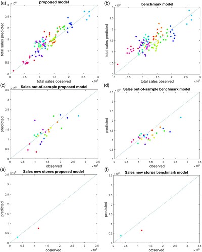
The upper left panel of Figure 3 graphs the in-sample store sales predictions using the proposed model for the 102 store-time observations that have been used for estimation over a period of four years, and the upper right panel their counterparts using the benchmark model explaining total sales directly. The average absolute prediction error over these 102 observations is €179,870 for the proposed model compared with €272,700 for the benchmark model, which represents a reduction of 34%. The correlation coefficient between observed and predicted sales equals 0.63. This correlation coefficient decreases to 0.60 when the trade area is reduced to zip codes responsible for 75% of total sales and to 0.51 when the trade area is enlarged to zip codes responsible for 95% of total sales. We therefore conclude that the focus on the primary and secondary zones of a store’s trade area (85% of total sales) produces the best results from a forecasting point of view.

The left and right centre panels of Figure 3 graph the out-of-sample store sales forecasts of the proposed and benchmark models one year ahead for the 26 existing stores in the hold-out sample. The average absolute prediction error over these stores is €258,330 for the proposed model compared with €272,130 for the benchmark model, which represents a reduction of 5%.

To illustrate how the retailer might use the results also for the evaluation of new store locations, we use the estimated coefficients from Tables 4 and 5 to forecast each sales component for two new stores that were opened and employ the obtained values to calculate their (potential) sales. The bottom left and right panels of Figure 3 graph the store sales predictions of the proposed and benchmark models for these two stores. The mean absolute prediction error over these stores amounts to €213,200 for the proposed model, compared with €287,820 for the benchmark model, which represents a reduction of 26%.

In summary, we conclude that the proposed model outperforms the benchmark model in each of these three prediction scenarios, indicating that our modelling approach provides retailers with a useful tool for evaluation existing stores and finding new store locations.

By comparing the predicted and observed sales figures for each four-digit zip code, the retailer also can identify areas in which it can improve store performance. Our model predicts three sales components (i.e., loyalty card penetration rate, visit frequency and average expenditures per visit) for each zip code in the store’s trade area. Using the predicted values for each sales component, we calculate total sales to loyalty card holders for each zip code and compare these values to the realized sales figures. Figure A1 in Appendix A in the supplemental data online plots the predicted values for each sales component (panels a–c) and the total sales to loyalty programme members (panel d) for the trade area of one of two stores that opened recently. Because the retailer may want to know whether the store is currently over- or underperforming in certain areas, we further plot the difference between the observed and predicted values for each sales component (panels e–h).

Panel (a) confirms that the loyalty card penetration rate relates negatively to distance to the store, apart from the north-eastern part of the trade area in which a large city is located and where the number of loyalty card holders is substantially lower than in other zip codes at similar distances to the store. Visit frequency also decreases with distance to the store (panel b), meaning that loyalty card holders living closer to the store visit it more often than do those living farther away. Average expenditures per visit increase with distance to the store (panel c), because members who live farther away buy in larger quantities and are more likely to travel by car. This finding holds true for the largest part of the trade area but, again, not for the north-eastern part of the market, for which we predict relatively low expenditures per visit. From panel (d) we note that if any relationship exists between total sales to loyalty card holders and travel distance, it tends to be negative, which indicates that the negative relationships between the loyalty card penetration rate and visit frequency and distance dominate the positive relationship between average expenditures and travel distance. Panel (e) illustrates that the loyalty card penetration rate of the new store is lower than predicted in a large part of its trade area. The retailer might try to enhance the number of loyalty card holders by, for example, mailing a door-to-door flyer that informs potential customers about the advantages of the store and its loyalty programme. The outlet manager could investigate the local situation further by, for example, conducting a customer survey. Combined with the model results, which help explain the causes for the (negative) differences in sales, the manager could use information from the survey to develop marketing strategies specifically for certain store locations or even certain zip codes.

DISCUSSION AND CONCLUSIONS

Store location is crucial to store performance because it determines store attractiveness and thus consumers’ shopping decisions and spending patterns. The key objective of this paper is to provide a general modelling approach to store location evaluation based on geographical consumer information, both for existing and new locations. The proposed model contributes to store location literature in two important ways. First, we use a decomposition framework to split store sales into their constituent parts, which leads to insights that remain unavailable with a model of just sales. Second, we account for random effects and spatial autocorrelation which, by borrowing information from past and neighbouring observations, turns out to be considerably better at predicting sales performance than a model that ignores these effects. We also discuss and show how to estimate these models using longitudinal data pertaining to stores, purchase behaviour and consumer demographics.

In the empirical study we apply our decomposition framework to clothing stores of a Dutch retail chain. The customer database, supplemented with survey data describing the retail environment of individual stores and commercially available geodemographic information, enables us to estimate random effects and spatial error random models that explain a substantial amount of variance in store sales. We identify several important drivers of store sales, such as travel distance, number of double-income families and assortment composition, and find that their impact is different from one sales component to another. We also find empirical evidence of random effects and spatial dependence between the observations for each sales component respectively over time and among zip codes, caused by unobserved similarities in sociodemographic and economic circumstances, such as region-specific lifestyle characteristics and consumer preferences and local road and public transport networks.

The finding that the predictive performance of our decomposition model outperforms its counterpart of the benchmark model that explains total sales directly underlines its usefulness for store location and evaluation decisions. Retailers who consider a number of candidate locations may want to use our model to obtain estimates of potential sales for each site, which they can use to decide whether or not to invest in potential locations.

One limitation of our study might be that some of the findings are peculiar to the retailer under consideration. In line with the Central Place Theory, the kind of drivers to be included, as well as their signs, magnitudes and significance levels may be different from one retailer to another. Clothing is a commodity for which consumers prefer comparative shopping and are willing to travel further than for, say, groceries. Likewise, the effect of the number of competitors for clothing stores may be positive due to agglomeration effects, while it is unlikely for groceries. On the other hand, we have tried to present the model in such a general form that it can also be applied to other retailers or other settings that require evaluations of the location of facilities, such as health clubs, restaurants, banks, or public facilities. This is because the opportunities to decompose sales into different components and to explain and predict these components using random effects and spatial autocorrelation remain.

DISCLOSURE STATEMENT

No potential conflict of interest was reported by the authors.

REFERENCES

- Ailawadi, K. L., & Keller, K. L. (2004). Understanding retail branding: Conceptual insights and research priorities. Journal of Retailing, 80(4), 331–342. https://doi.org/https://doi.org/10.1016/j.jretai.2004.10.008
- Allaway, A. W., Berkowitz, D., & D’Souza, G. (2003). Spatial diffusion of a new loyalty program through a retail market. Journal of Retailing, 79(3), 137–151. https://doi.org/https://doi.org/10.1016/S0022-4359(03)00037-X
- Anselin, L. (1988). Spatial econometrics: Methods and models. Kluwer.
- Baltagi, B. H. (2005). Econometric analysis of panel data (3rd ed.). Wiley.
- Baltagi, B. H., Bresson, G., & Pirotte, A. (2012). Forecasting with spatial panel data. Computational Statistics & Data Analysis, 56(11), 3381–3397. https://doi.org/https://doi.org/10.1016/j.csda.2010.08.006
- Baltagi, B. H., & Li, D. (2004). Prediction in the panel data model with spatial correlation. In L. Anselin, R. J. G. M. Florax, & S. J. Rey (Eds.), Advances in spatial econometrics: Methodology, tools, and applications (pp. 283–295). Springer.
- Baltagi, B. H., & Li, D. (2006). Prediction in the panel data model with spatial correlation: The case of liquor. Spatial Economic Analysis, 1(2), 175–185. https://doi.org/https://doi.org/10.1080/17421770601009817
- Bell, D. R. (2014). Location is still everything: The surprising influence of the real world on how we search, shop, and sell in the virtual one. New Harvest.
- Bell, D. R., Ho, T.-H., & Tang, C. S. (1998). Determining where to shop: Fixed and variable costs of shopping. Journal of Marketing Research, 35(3), 352–369. https://doi.org/https://doi.org/10.1177/002224379803500306
- Bell, D. R., & Song, S. (2007). Neighborhood effects and trial on the internet: Evidence from online grocery retailing. Quantitative Marketing and Economics, 5(4), 361–400. https://doi.org/https://doi.org/10.1007/s11129-007-9025-5
- Bhatnagar, A., & Ratchford, B. T. (2004). A model of retail format competition for non-durable goods. International Journal of Research in Marketing, 21(1), 39–59. https://doi.org/https://doi.org/10.1016/j.ijresmar.2003.05.002
- Bradlow, E. T., Bronnenberg, B., Russell, G. J., Arora, N., Bell, D. R., Duvvuri, S. D., Hofstede, F. T., Sismeiro, C., Thomadsen, R., & Yang, S. (2005). Spatial models in marketing. Marketing Letters, 16(3–4), 267–278. https://doi.org/https://doi.org/10.1007/s11002-005-5891-3
- Breusch, T. S. (1987). Maximum likelihood estimation of random effects models. Journal of Econometrics, 36(3), 383–389. https://doi.org/https://doi.org/10.1016/0304-4076(87)90010-8
- Briesch, R. A., Chintagunta, P. K., & Fox, E. J. (2009). How does assortment affect grocery store choice? Journal of Marketing Research, 46(2), 176–189. https://doi.org/https://doi.org/10.1509/jmkr.46.2.176
- Bronnenberg, B. J. (2005). Spatial models in marketing research and practice. Applied Stochastic Models in Business and Industry, 21(4–5), 335–343. https://doi.org/https://doi.org/10.1002/asmb.565
- Buckner, R. W. (1998). Site selection: New advancements in methods and technology. Lebhar-Friedman.
- Campo, K., & Gijsbrechts, E. (2004). Should retailers adjust their micro-marketing strategies to type of outlet? An application to location-based store space allocation in limited and full-service grocery stores. Journal of Retailing and Consumer Services, 11(6), 369–383. https://doi.org/https://doi.org/10.1016/j.jretconser.2003.12.003
- Chan, T. Y., Padmanabhan, V., & Seetharaman, P. B. (2007). An econometric model of location and pricing in the gasoline market. Journal of Marketing Research, 44(4), 622–635. https://doi.org/https://doi.org/10.1509/jmkr.44.4.622
- Chintagunta, P. K., Erdem, T., Rossi, P. E., & Wedel, M. (2006). Structural modeling in marketing: Review and assessment. Marketing Science, 25(6), 604–616. https://doi.org/https://doi.org/10.1287/mksc.1050.0161
- Del Gatto, M., & Mastinu, C. S. (2018). A Huff model with firm heterogeneity and selection. Application to the Italian retail sector. Spatial Economic Analysis, 13(4), 442–456. https://doi.org/https://doi.org/10.1080/17421772.2018.1451914
- De Mello-Sampayo, F. (2016). A spatial analysis of mental healthcare in Texas. Spatial Economic Analysis, 11(2), 152–175. https://doi.org/https://doi.org/10.1080/17421772.2016.1102959
- Duan, J. A., & Mela, C. F. (2009). The role of spatial demand on outlet location and pricing. Journal of Marketing Research, 46(2), 260–278. https://doi.org/https://doi.org/10.1509/jmkr.46.2.260
- Elhorst, J. P. (2005). Unconditional maximum likelihood estimation of linear and log-linear dynamic models for spatial panels. Geographical Analysis, 37(1), 85–106. https://doi.org/https://doi.org/10.1111/j.1538-4632.2005.00577.x
- Elhorst, J. P. (2014). Spatial econometrics: From cross-sectional data to spatial panels. Springer.
- Elhorst, J. P. (2017). Spatial models. In P. S. H. Leeflang, J. E. Wieringa, T. H. A. Bijmolt, & K. H. Pauwels (Eds.), Advanced methods for modelling markets (pp. 173–202). Springer.
- Fingleton, B. (2009). Prediction using panel data regression with spatial random effects. International Regional Science Review, 32(2), 195–220. https://doi.org/https://doi.org/10.1177/0160017609331608
- Gauri, D. K., Pauler, J. G., & Trivedi, M. (2009). Benchmarking performance in retail chains: An integrated approach. Marketing Science, 28(3), 502–515. https://doi.org/https://doi.org/10.1287/mksc.1080.0421
- González-Benito, O., & González-Benito, J. (2005). The role of geodemographic segmentation in retail location strategy. International Journal of Market Research, 47(3), 295–316. https://doi.org/https://doi.org/10.1177/147078530504700305
- Goulard, M., Thibault, L., & Thomas-Agnan, C. (2017). About predictions in spatial autoregressive models: Optimal and almost optimal strategies. Spatial Economic Analysis, 12(2–3), 304–325. https://doi.org/https://doi.org/10.1080/17421772.2017.1300679
- Hartmann, W. R., Manchanda, P., Nair, H., Bothner, M., Dodds, P., Godes, D., Hosanagar, K., & Tucker, C. (2008). Modeling social interactions: Identification, empirical methods and policy implications. Marketing Letters, 19(3–4), 287–304. https://doi.org/https://doi.org/10.1007/s11002-008-9048-z
- Jank, W., & Kannan, P. K. (2005). Understanding geographical markets of online firms using spatial models of customer choice. Marketing Science, 24(4), 623–634. https://doi.org/https://doi.org/10.1287/mksc.1050.0145
- Kalnins, A. (2004). An empirical analysis of territorial encroachment within franchised and company-owned branded chains. Marketing Science, 23(4), 476–489. https://doi.org/https://doi.org/10.1287/mksc.1040.0082
- Kato, T. (2008). A further exploration into the robustness of spatial autocorrelation specifications. Journal of Regional Science, 48(3), 615–639. https://doi.org/https://doi.org/10.1111/j.1467-9787.2008.00566_1.x
- Kelejian, H. H., & Prucha, I. R. (2007). The relative efficiencies of various predictors in spatial econometric models containing spatial lags. Regional Science and Urban Economics, 37(3), 363–374. https://doi.org/https://doi.org/10.1016/j.regsciurbeco.2006.11.005
- Kivetz, R., & Simonson, I. (2003). The idiosyncratic fit heuristic: Effort advantage as a determinant of consumer response to loyalty programs. Journal of Marketing Research, 40(4), 454–467. https://doi.org/https://doi.org/10.1509/jmkr.40.4.454.19383
- Kumar, V., & Karande, K. (2000). The effect of retail store environment on retailer performance. Journal of Business Research, 49(2), 167–181. https://doi.org/https://doi.org/10.1016/S0148-2963(99)00005-3
- Leenheer, J., & Bijmolt, T. H. A. (2008). Which retailers adopt a loyalty program? An empirical study. Journal of Retailing and Consumer Services, 15(6), 429–442. https://doi.org/https://doi.org/10.1016/j.jretconser.2007.11.005
- Leenheer, J., van Heerde, H. J., Bijmolt, T. H. A., & Smidts, A. (2007). Do loyalty programs really enhance behavioral loyalty? An empirical analysis accounting for self-selecting members. International Journal of Research in Marketing, 24(1), 31–47. https://doi.org/https://doi.org/10.1016/j.ijresmar.2006.10.005
- LeSage, J. P., & Pace, R. K. (2009). Introduction to spatial econometrics. Taylor and Francis.
- Levy, M., & Weitz, B. A. (2004). Retailing management. McGraw-Hill/Irwin.
- Miller, D. M. (1984). Reducing transformation bias in curve fitting. American Statistician, 38, 124–126. https://doi.org/https://doi.org/10.1080/00031305.1984.10483180
- Öner, Ö. (2017). Retail city: The relationship between place attractiveness and accessibility to shops. Spatial Economic Analysis, 12(1), 72–91. https://doi.org/https://doi.org/10.1080/17421772.2017.1265663
- Pan, Y., & Zinkhan, G. M. (2006). Determinants of retail patronage: A meta-analytical perspective. Journal of Retailing, 82(3), 229–243. https://doi.org/https://doi.org/10.1016/j.jretai.2005.11.008
- Reinartz, W. J., & Kumar, V. (1999). Store-, market-, and consumer-characteristics: The drivers of store performance. Marketing Letters, 10(1), 5–23. https://doi.org/https://doi.org/10.1023/A:1008011622335
- Seim, K. (2006). An empirical model of firm entry with endogenous product-type choices. The RAND Journal of Economics, 37(3), 619–640. https://doi.org/https://doi.org/10.1111/j.1756-2171.2006.tb00034.x
- Singh, V. P., Hansen, K. T., & Blattberg, R. C. (2006). Market entry and consumer behavior: An investigation of a Wal-mart supercenter. Marketing Science, 25(5), 457–476. https://doi.org/https://doi.org/10.1287/mksc.1050.0176
- Steenburgh, T. J., Ainslie, A., & Engebretson, P. H. (2003). Massively categorical variables: Revealing the information in zip codes. Marketing Science, 22(1), 40–57. https://doi.org/https://doi.org/10.1287/mksc.22.1.40.12847
- Thomadsen, R. (2007). Product positioning and competition: The role of location in the fast food industry. Marketing Science, 26(6), 731–741. https://doi.org/https://doi.org/10.1287/mksc.1070.0338
- Van Heerde, H. J., & Bijmolt, T. H. A. (2005). Decomposing the promotional revenue bump for loyalty program members versus nonmembers. Journal of Marketing Research, 42(4), 443–457. https://doi.org/https://doi.org/10.1509/jmkr.2005.42.4.443
- Verbeek, M. (2000). A guide to modern econometrics. Wiley.
- Vroegrijk, M., Gijsbrechts, E., & Campo, K. (2016). Battling for the household’s category buck: Can economy private labels defend supermarkets against the hard-discounter threat? Journal of Retailing, 92(3), 300–318. https://doi.org/https://doi.org/10.1016/j.jretai.2016.05.003
- Yang, S., & Allenby, G. M. (2003). Modeling interdependent consumer preferences. Journal of Marketing Research, 40(3), 282–294. https://doi.org/https://doi.org/10.1509/jmkr.40.3.282.19240