Integrating digital and global transformations in forecasting regional growth: the MASST5 model

ABSTRACT

During the past decade, world economic development was coupled with disruptive challenges. Among them, digitalisation and new forms of globalisation represent a potential threat for economic growth opportunities and for the future of labour markets. Digital transition calls for the assessment of the impact of robotisation and digitalisation on skill composition, employment levels, productivity and growth dynamics. In turn, the largest wave of globalisation after that taking place before the First World War caused, first, the emergence of global value chains and, more recently, their disintegration with partial mechanisms of reshoring, with consequences for growth and employment opportunities. All these challenges call for comprehensive approaches to their modelling. This paper presents the main advances introduced in the fifth generation of the MAcroeconomic, Sectoral, Social, Territorial (MASST5) model, which carved a relevant niche in the empirical literature on macro-econometric regional growth, and has now been strengthened to model future digitalisation transitions, as well as the national and regional breakdown of the way global value chains will reorganise. A longer time series, especially in the regional submodel, also allows one to take the major changes taking place in Europe following the 2007–08 financial crisis, and the 2020 COVID-induced contraction into account.

KEYWORDS:

• macro-econometric regional growth
• digital transformations
• global value chains
• territorial spillovers

JEL:

• O11
• R11
• R12

1. INTRODUCTION

During the past decade, world economic development was coupled with disruptive challenges. Among them, digitalisation and new forms of globalisation represent a potential threat for economic growth opportunities and for the future of labour markets. Digital transition calls for the assessment of the impact of robotisation and digitalisation on skill composition, employment levels, productivity and growth dynamics. In turn, the largest wave of globalisation after the one taking place before the First World War first caused the emergence of global value chains (GVCs) and, more recently, their disintegration with partial mechanisms of reshoring, with consequences for growth and employment opportunities.

These challenges are radically changing the mode of production and the structure of international trade. On the one hand, globalisation is increasing in intensity; on the other, it is also changing the way it is enacted, with faster and more radical shifts in the nature of GVCs, and in the relative positioning of industries and regions within the global scene. Moreover, these challenges are often intertwined, and potentially exacerbated by structural instability on international markets, due to further exogenous shocks such as the recent COVID-19 pandemic in spring 2020, and, more recently, the surge in energy prices preceding the Russia–Ukraine conflict. On a longer horizon, such mega-trends may be exacerbated by further challenges, such as climate change and global warming, the increasing instability in global geopolitics, the 4.0 technological paradigm, and the diffusion of populism, whose consequences need to be accounted for in regional forecasting models.

With the goal of understanding the determinants of these mega-trends, and, more importantly, their long-run economic consequences, several macro-econometric models have been introduced in the scientific debate. In regional economics, the debate has been crystallising around spatial computable general equilibria (SCGEs). While they present several conceptual and methodological advantages, their structures do not appear suitable for dealing with an empirical assessment of the effects of mega-trends. In fact, by their very nature, SCGEs are meant to assess the effects of single-market shocks, whose long-run impact can be elegantly captured with impulse response functions. However, they are ill-suited at capturing the effects of multiple shocks simultaneously taking place on multiple markets. On the other hand, other approaches built to reflect about the long-run implications of complex scenarios characterised by multiple shocks on numerous markets are typically qualitative in nature, and fall short of actually quantifying the economic consequences of such scenarios.

In order to quantify the complex – and often well-entangled – economic impacts of multiple shocks on different markets, a tool capable of simulating multiple shocks in the medium and long run at a regional level is needed. One such macro-econometric model is called MAcroeconometric, Social, Sectoral, Territorial (MASST). It merges macro-economic elements with territorial features for forecasting regional growth trajectories. It was created in 2005 (Capello, 2007) with the aim to overcome the dichotomous approaches interpreting regional growth either as a bottom-up process without macro-economic elements, or as a top-down one, whereby national growth rates are reassigned to regions according to their weights, neglecting any role to regional propulsive forces. While this model has reached its fourth generation (Capello & Caragliu, 2021a), its structure fell short of a fully fledged modelling of the effects of some of the mega-trends above anticipated, including the emergence of GVCs, and rapid technological change which goes under the 4.0 technological revolution umbrella.

This paper introduces the fifth generation of the MASST model (MASST5). MASST5 presents substantial improvements along many lines with respect to previous versions. Its structure has been strengthened to model two relevant challenges, that is, the 4.0 technological revolution and globalisation. The choice of these two mega-trends is due to their particular influence on global labour markets, mostly induced by fast diffusion of labour-saving technologies and by the job-creation effect of nearshoring and back-shoring of GVCs, spurring a wave of empirical studies assessing the impact of 4.0 technologies and GVCs reorganisation on skill composition, employment levels, growth and productivity growth (Camagni et al., 2022). On the theoretical front, GVCs are for the first time introduced in the model in both the national and the regional submodels. Moreover, MASST5 now also allows one to simulate long-run impacts of 4.0 technological change in both manufacturing and tertiary activities. At the same time, enhanced data availability allows one to exploit longer time series in the process of estimating the model parameters, thereby leading to more accurate forecasting of long-run regional economic growth rates.

The paper is structured as follows. Section 2 frames the MASST5 model within the broader literature on regional macro-econometric growth models. It concludes with the main advantages stemming from the use of our approach. Section 3 documents the structure of the MASST model. Section 4 illustrates the fifth generation’s main novelties.¹ Section 5 proceeds by illustrating the main indicators used to introduce the novelties of the model, while also providing a comprehensive discussion of the data set assembled. Section 6 provides a critical comment of the empirical results concerning the model’s new features. Lastly, Section 7 concludes by drawing some lessons from the model, as well as by illustrating future research directions concerning potential scenario applications.

2. THE VALUE ADDED OF A SCENARIO-BUILDING MODEL

Over the past decade, several substantial advances appeared in the literature on multi-equation regional growth models that are here worth summarising, in particular with the goal of addressing the complex challenges previously discussed.

Up to the first decade of this century, the scientific debate on multi-equation models was characterised by a dichotomy between top-down and bottom-up tools. This traditional dichotomy is well reflected in the excellent literature review presented by Harris (2011), and also shapes the synthesis of the scientific debate presented in prior versions of the MASST model (e.g., Capello & Caragliu, 2021a).

Top-down models include the very first generation of multi-equation regional growth models. This class of models typically simulated regional growth rates on the basis of weights distributing national growth rates to the areas comprised in the country itself. This, for instance, applies to Bell (1967), representing one of the earliest attempts to extend our understanding of subnational growth processes beyond the (by then) already standard input–output tables. In particular, this model goes beyond the two equation systems that previously led competing models to mostly derive aggregate regional employment and income multipliers. In particular, the Bell model endogenised various types of income, capital stock, investment, aggregate employment, population, unemployment rates and migration rates for the US state of Massachusetts. In this early attempt, the focus on a single state led to structurally avoiding the interdependencies among proximate areas, and the single state analysed was treated on the basis of the economic base approach (i.e., economic growth was triggered by external demand).

The main purpose of bottom-up models was instead to capture the effect of region-specific factors on regional growth rates, thereby partially neglecting the otherwise paramount relevance of country-level factors. Multi-equations tools followed a fertile theoretical debate across the regional science and economic geography literatures for a couple of decades (Stöhr & Taylor, 1981), suggesting the growing importance of region-specific characteristics and territorial features in driving long-run regional development. In contrast to top-down approaches, where regional growth is modelled as a competitive process, in bottom-up models regional development takes place through generative processes (Camagni, 2002). In this class of models, a region overperforming causes faster growth rates for the country where it is located: ‘agglomeration economies and spatial clustering of activities may induce more output than if production is dispersed  …  and additional growth may come from improvements in spatial efficiency rather than from additional factor inputs’ (Richardson, 1978, p. 146).

While examples of purely generative regional growth models are rather scant, it is safe to conclude that the generative nature of regional growth is now well established and that localised increasing returns are now a standard assumption triggering regional growth in formal models (Fujita & Thisse, 2002; McCann & Van Oort, 2019).

Since the mid-1980s, the emergence of computable general equilibrium (CGE) models was first complemented with their application to regional contexts and datasets, next with their extension to formally take spatial heterogeneity into account (spatial CGE – SCGE).² SCGEs are based on the concept of Walrasian general equilibrium, whereby all markets relevant for a given economy clear:

The three conditions of market clearance, zero profit and income balance are employed by CGE models to solve simultaneously for the set of prices and the allocation of goods and factors that support general equilibrium. The three conditions define Walrasian general equilibrium not by the process of exchange by which this allocation comes about, but in terms of the allocation itself. (Wing, 2004, p. 5)

SCGEs brought substantial advances with respect to the scientific context they were first developed in. Among those are the following:

• SCGEs focus explicitly on the microfoundations of the behaviour of individuals within each market, making reasonable (and, again, explicit) assumptions on how individuals cause equilibria on the markets.

• In SCGEs, all relevant markets are assumed to clear.

• Consequently, impulse response functions can be calculated to simulate region-specific reactions to individual policy shocks, which provides for a solid toolbox to ex ante assess regional policies.

In the European context, eminent examples of SCGEs include the Rhomolo model used by the Joint Research Center (JRC) of the European Union as a policy assessment tool for EU policies (Brandsma et al., 2015); the GMR model (Varga, 2017); and the EU – EMS model (Ivanova et al., 2019a). Outside the EU, other examples of SCGEs include the FEDERAL-F model (Giesecke, 2002) for Australia; the TERM model (Chen, 2019) for China; Hansen and Johansen (2017) for Norway; B-MARIA-27 for Brazil (Haddad & Hewings, 2005); and, to a partial extent due to its eclectic nature, the REMI model (Treyz et al., 1992) (on the more heterodox approach undertaken in this model, see also the excellent review of SCGEs by Partridge & Rickman, 1998).

The literature so far discussed documented a period of substantial improvement in our understanding of long-run regional growth mechanisms that has translated into significantly more accurate economic forecasts. In particular, SCGEs present:

flexibility in terms of a firm’s production function and a household’s utility function depending on the purpose of the analysis; resource constraints; calculation of the behavior of consumers; and the provision of price information in equilibrium [whereby] None of these characteristics can be considered and observed using an I-O analysis. (Tatano & Tsuchiya, 2008, p. 255)

While having become standard in impact assessment, SCGEs present a relevant structural limitation in their strong assumption of economic systems quickly transitioning towards a new steady state once a prior general equilibrium is perturbed by an idiosyncratic shock.

Over the past few years, SCGEs have been further strengthened by exploiting Bayesian techniques for the estimation of structural parameters. The adoption of Bayesian methodologies in simulating long-run growth rates is often preferred to classical statistics, mostly on the basis of superior performance in long-run forecasting (Geweke, 2001).³ For this reason, several models forecasting national or regional growth in the very long run adopt a Bayesian structure (see, e.g., Müller et al., 2022, for a recent example and a review).

Within this landscape, an additional development took place over the past decade, related to the diffusion of agent-based models (ABMs) for forecasting regional growth rates. ABMs have a long-standing tradition also in other branches of economics, as well as in other disciplines, such as computer science, where they are known as multi-agent systems (MAS), or ecology, where they are labelled individual-based modelling (Axtell & Farmer, 2022). In regional economics, ABMs are increasingly adopted for their capacity to overcome somewhat oversimplifying assumptions often made in multi-equations regional growth models in order to ensure analytical tractability. This means that ABMs present in their turn substantial perks with respect to competing approaches:

• ABMs present a more explicit and self-conscious approach to modelling interactions among complex systems and interactions among agents, often portrayed as characterised by bounded rationality.

• The calibration of ABMs often takes place through dedicated surveys or census data sets, which enhances the explanation of behavioural characteristics of the actors being modelled (Clarke, 2014).

Before their relatively recent diffusion in regional science, ABMs were often criticised due to their alleged worse performance in terms of out-of-sample forecasting. Moreover, further criticism arose due to their very nature of fitting more complex definitions of rationality, which on the one hand makes them more capable of modelling complex systems, but, on the other hand, would essentially make them capable of explaining nearly any stylised fact, provided an appropriate specification of behavioural models would be adopted.

The first criticism has been recently overcome with Poledna et al. (2023), who propose an ABM model that performs similarly to a CGE estimated with Bayesian techniques in terms of out-of-sample forecasting. The second critique remains outstanding, but evidently does not prevent this literature to increasingly invest in these tools, due to their capacity to take account of economic complexity.

The whole literature on multi-equations regional growth models appears, especially in its last decade developments, to focus on purposes that are rather orthogonal to what a quantitative scenario model aims to achieve. In particular, SCGEs and ABMs focus on modelling complex equilibria and, consequently, on assessing the impact of specific shocks on individual markets on overall equilibrium levels. These two classes of models appear instead less amenable to simulating the quantitative effects of scenarios.

Scenarios can be defined as:

a description of a possible future state or condition within a subject field. Scenarios are not predictions of future events, and although they sometimes provide probabilities, their main function is to present decision makers with a set of alternative futures against which different courses of action might be measured. (Johansen, 2018, p. 116)

In this sense, the MASST model is set at the crossing of the economics literature aiming at quantifying point forecasts, and the qualitative literature dealing with long-run foresights. The latter can instead be defined as ‘readiness to deal with long-term issues (especially on the part of governments)’. This approach to forecasting regional growth has been previously termed quantitative foresight (Camagni & Capello, 2012), and appears useful in making sense of the complex potential economic consequences of multiple shocks simultaneously taking place, including the global challenges anticipated in section 1. By the same token, with the goal to model the long-run consequences of mega-trends simultaneously shocking multiple markets, models such as MASST, using econometrically estimated parameters, appear more amenable to modelling off-equilibrium growth patterns than models whose parameter structure is mostly calibrated on the basis of theoretical toolboxes built on the concept of equilibrium.

3. LOGICAL STRUCTURE OF THE MASST5 MODEL

The MASST model is a macro-econometric regional growth model built to simulate regional growth in the medium and long run. The acronym contains the different dimensions (macro-economic, sectoral, social and territorial) on which the model is built. While the first version of the model is presented in detail by Capello (2007), the model has undergone several substantial improvements over the past 15 years (Capello et al., 2017; Capello & Caragliu, 2021a; Capello & Fratesi, 2012), and has been applied to simulate the effects of several complex scenarios, as well as the impacts of multiple exogenous shocks.⁴

MASST belongs to the macro-class of regional macro-econometric growth models. In this sense, it is a pretty traditional model, in that model parameters are econometrically estimated, following in the footsteps of the Cowles Commission approach to identification.⁵ More specifically, in the MASST model, regional growth is explained by a combination of national (macro-economic) and regional (structural) factors.

The national submodel is based on Keynesian quasi-identities explaining the growth of aggregate income, consumption, public expenditure, exports and imports, thereby modelling aggregate demand. With the aim to explain the differential growth rate of a region with respect to its nation, the regional submodel, instead, captures the supply side, depicting the sectoral, social and territorial aspects characterising the region by:

• quantifying tangible and intangible elements, that is, different assets of territorial capital (Camagni, 2019), especially those with an intangible nature, linked to actors’ perceptions, relational elements, and cooperation attitudes; and

• analytically formulating territorial complexity, that is, the set of context specificities and synergies that characterise regional growth.⁶

The model runs across two stages:

• In the estimation stage, structural relations between explanatory and dependent variables in various national and regional equations are estimated over a long run time span through a set of equations included in the model.

• In the simulation stage, estimated coefficients are employed for simulating likely future growth patterns (usually, over a 15–20-year horizon), and given an internally coherent sets of assumptions forming regional growth scenarios.

The model merges national and regional growth-enhancing factors by explaining regional growth ($\mathrm{\Delta }{Y}_r$) as a decomposition between a national growth rate ($\mathrm{\Delta }{Y}_C$) and a regional differential shift (s) (Capello, 2007): (1) $\mathrm{\Delta }{Y}_r=\mathrm{\Delta }{Y}_C+sr\in N$(1) where r indicates a region, with r = 1, … , 281, C is the country it belongs to, and N indicates the total number of regions analysed. The shift s in equation (1) is represented at the core of Figure 1, depicting the logical structure of the model. In Figure 1, individual model equations are represented with shaded grey areas. Within each equation, Figure 1 shows two types of shapes:

• Octagons, representing variables exogenous to the model. For these variables, the model does not produce forecasts, and their value is used by the modeler as a long-run target to which initial values of each variable tend.

• Rounded-angled shapes, that represent instead variables endogenous to the model. These dependent variables are simulated by the model, and may enter the specification of other endogenous variables, or instead represent final outcomes of the simulation exercise.

Figure 1. Logical structure of the MASST5 model.

Source: Authors’ elaboration.

Logical structure of the MASST5 model, with left-hand side shapes representing the national submodel, and right-hand side shapes representing the regional submodel.

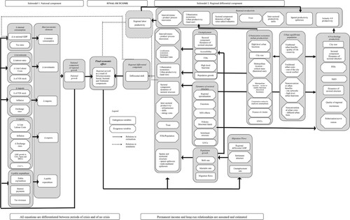
In Figure 1, the left-hand side represents the national submodel, while the right-hand side encompasses regional submodel equations.

The logical structure of the model foresees creating a comprehensive set of assumptions on all exogenous variables of the model. This combination is the quantitative translation of a scenario – a blend of hypotheses on mega-trends in all sectors of national and regional economies that need to be based on solid and internally coherent thinking about likely developments in the macro and local spheres.

Translated into quantitative variables, assumptions are included in the model as targets (T) to which an independent variable (x) tends over the period t − 1 and t with a speed of adjustment (s): (2) $x_t=x_{t-1}+s(T-x_{t-1})+s$(2) where s denotes the speed of adjustment. As s approaches 1, the exogenous variable approaches the target value faster (so that, hypothetically, when s = 1 the speed of adjustment is instantaneous). In MASST5, targets can be set also differently for different combinations of countries or typologies or regions.

One last word relates to the outcomes of the model. MASST5 predicts the following results for all NUTS-2 regions in Europe, with a major effort for the fifth generation of the model to readjust the NUTS classification to its more recent 2016 version, leading to the inclusion of all 281 administrative units, including overseas territories:⁷

Outcomes of simulation exercises must be interpreted differently from the results of SGCE simulations. While MASST5 does produce point forecasts about all variables in Table 1, including regional GDP growth rates, their magnitude is to be compared across regions, rather than being interpreted as precise assessments; in this sense, quantitative foresights strike a balance between long-run qualitative foresights, whose diffusion has been relatively slowed down by a ‘paucity of grounded hypotheses about scenario planning and still insufficient empirical field data to test its core premises’ (Schoemaker, 2021, p. 1), and quantitative forecasts.

Table 1. MASST5 simulated outcomes (endogenous variables).

Block of the model	MASST5 simulation outcomes
National	Gross domestic product (GDP) growth
	Consumption growth
	Public expenditure growth
	Investment growth
	Export growth
	Import growth
Regional/urban	Regional GDP growth
	Manufacturing employment growth
	Service employment growth
	Unemployment rates
	Migration rates
	Urban land rent (dynamic agglomeration economies)
	Equilibrium urban population
	Regional labour productivity
	Labour productivity growth in 4.0 sectors
	Regional population

In the next section, the generic structure description will be further tailored in terms of the advances of the new generation of the MASST model.

4. ADVANCES IN THE MASST5 MODEL

This paper documents the major steps forward made with the MASST model with its fifth generation. These changes incorporate in the simulation capacity of the model two of the major challenges taking place in European regional economies, namely the changing technological paradigm related to the 4.0 technological revolution, and the evolving nature, structure and pervasiveness of GVCs.

4.0 technologies are an overarching label comprising wide-ranging technological fields, such as artificial intelligence, robotics, internet of things, autonomous vehicles, 3D printing, sensors, nano-technologies, biotechnology, energy storage, etc. (Brynjolfsson & McAfee, 2014; Schwab, 2016). 4.0 Technologies are expected to lead to drastic socio-economic changes, on the one hand, leading to new sources of productivity gains, but on the other, generating new threats for local labour markets, thereby possibly reinforcing pre-existing inequalities. At the regional level, adverse outcomes of the adoption of 4.0 technologies, along with spatially heterogeneous impacts, have already been documented by Capello and Lenzi (2021a, 2021b). The capacity to simulate regional impacts of this technological revolution is a first relevant theoretical addition to the model.

Technically, the model incorporates 4.0 technologies following Capello and Lenzi (2021a). In particular, we include data on labour productivity of six clusters of industries based on their different degree of potential exploitation of 4.0 technologies. Six clusters of technology, induced, and carrier sectors are obtained according to (Capello & Lenzi, 2021a):

• Their degree of digitalisation.

• Their potential gains obtained by the introduction of 4.0 technologies, measured through the presence of the particular input factor (‘key factor’ as labelled in Perez, 1983) – the digital elaboration and transmission of large volumes of data, information, communication and texts – which is most affected in terms of cost abatement by the new technologies. The intensity of the key factor makes the adoption of the new technologies particularly profitable.

Sectoral labour productivity growth is expected to be influenced, first of all, by the intensity of adoption of 4.0 technologies in that industry (4.0 tech). This effect may vary according to the degree of specialisation of the region in that sector, as suggested by the interaction term (tech*SPEC IND). Last, but not least, this effect is measured controlling for the technological transformation prevailing in the region (D_techtransf). The latter is obtained through a cluster analysis on sectoral specialisation and technological adoption rates, identifying five different technological transformations: Industry 4.0, Digital service economy, Digitalisation of traditional services, Robotisation of traditional manufacturing and Niches of robotisation.⁸ Moreover, in equation (3) we also control for urbanisation economies (urbec); regional quality of government (QoG); human capital (HC); foreign direct investments (FDIs); specialisation in industry clusters (SPEC IND); and initial labour productivity (labprod): (3) $\begin{array}{rl}& \mathrm{\Delta }\mathrm{labpro}{d}_{i,r,t}={\beta }_1\mathrm{urbe}{c}_{r,t-1}+{\beta }_2\mathrm{Qo}{G}_{r,t-1}+{\beta }_{3}H{C}_{r,t-1}+{\beta }_4\mathrm{FD}{I}_{r,t-1}+{\beta }_{5}4.0\mathrm{tec}{h}_{i,r,t-1}+\\ & {\beta }_6\mathrm{SPEC}\mathrm{IN}{D}_{i,r,t-1}+{\beta }_{7}4.0\mathrm{tec}{h}_{i,r,t-1}\ast \mathrm{SPEC}\mathrm{IN}{D}_{i,r,t-1}+{\beta }_{8}D\mathrm{\_techtrans}{f}_{i,r,t}+{\beta }_9\mathrm{labpro}{d}_{i,r,t-1}+{\epsilon }_t\end{array}$(3) where indices r and t refer to the i-th region and t-th time period, respectively.

Predicted values of labour productivity in the six industry clusters i are then included as a control in the aggregate regional productivity regression, already introduced in MASST4 (Capello & Caragliu, 2021a). Among the six industry clusters, only the three predicted values that are significantly associated with aggregate regional productivity are included in this specification. This means that 4.0 technology’s impacts are interpreted as industry-specific shocks that enter the aggregate regional productivity regression.

This allows us to model 4.0 technological revolution shocks through:

• Changes in the intensity of robotisation in technology and induced manufacturing sectors.

• Changes in the intensity of online sales in carrier service sectors.

The notion of GVCs is not new to the scientific debate (Gereffi & Fernandez-Stark, 2016). Research on this topic took off after the seminal work by Hummels et al. (2001), and in correspondence with the highly debated third major wave of globalisation that took place over the past three decades (Dollar, 2001). GVCs are becoming increasingly more fragmented, which causes fragility and exposure to global shocks such as the COVID-19 pandemic and the new geopolitical tensions in Europe. While a rampant scientific debate raged on the fragmentation of GVCs at the macro-level (Timmer et al., 2014), much less is known about the regional breakdown of this fragmentation process (Bolea et al., 2022) despite the fact that the participation of regions in GVCs and the ensuing benefits are characterized by heterogeneity and warrant further in-depth examination (Capello et al., 2023). Moreover, how and where reorganisation will take place is unknown, and the future effects of the international organisation of production has to be analysed. MASST5 introduces the complexity of GVCs through indicators of the intensity and structure of GVCs at regional level. In the simulation stage, this also allows one to recalculate indicators based on scenario assumptions. These indicators have been calculated and introduced in the model on the basis of national and regional input–output trade in value added matrices (see also Section 5), for both the national and the regional submodels. In the former, we capture comparative advantages that countries have in international trade, and their participation in internationally fragmented production chains. For the regional part of MASST5, we model regional heterogeneity in the way regional economies participate in GVCs, which allows one to explain its differential growth with respect to the national level.

A third and last relevant advancement in MASST5 is related to the identification of a more nuanced period structure. In fact, due to the disruptive impact of the COVID-19 pandemic on regional economies (Capello & Caragliu, 2021b), a fourth period has been introduced in the estimation stage with respect to MASST4, which now allows one to choose among four period-specific parameters:

• 2004–08 (pre-crisis).

• 2008–12 (crisis).

• 2012–16 (post-crisis).

• 2016–20 (COVID-19).

In an econometrically estimated multi-equation regional growth model, time-changing coefficients allow to capture (possibly persistent) off-equilibrium situations, especially when repeated multiple simultaneous shocks affect regional economies. Evidence about the importance of this novelty comes whenever estimated coefficients change in a statistically significant manner over the estimation period; whenever available, this is presented in section 6. Data and indicators needed to translate these advances in the model are instead described in section 5.

5. DATA AND INDICATORS

5.1. The MASST5 data set

The MASST5 model is based on a unique database comprising three geographical levels (national, regional and urban). As anticipated above, we here present two main advances compared with previous versions. On the one hand, data update the time structure thanks to longer time series in order to simulate the impact of recent shocks (e.g., COVID-19). On the other hand, in MASST5 the ongoing digital and global transformations are modelled through indicators at both national and regional scales.

National data comprise the main determinants of the national accounts (i.e., consumption, investment, public expenditure, import and export) in a yearly panel setting covering the period 2000–20. The regional database covers the universe of EU NUTS-2 regions, including UK ones despite Brexit,⁹ with a panel structure based on four-year averages: pre-crisis (2004–08), crisis (2008–12), post-crisis (2012–16) and COVID-19 (2016–20).¹⁰ Finally, regarding the urban database, data for all NUTS-2 regions match the information of the largest city within the region (Camagni et al., 2016) allowing one to capture the urban dimension.

Tables A1 and A2 in Appendix A3 in the supplemental data online present the full list of variables included in the estimates discussed throughout the paper, together with their sources and time availability. Tables A1 and A2 also add whether variables are treated as endogenous or exogenous in the model (see also Table 1).

MASST5 simulates regional growth rates covering the period 2021–38. An 18-year simulation period allows one to both look at economic outcomes of scenario simulations into a decently long period ahead, without at the same time holding structural relationships among variables implausibly constant for a longer simulation period.

5.2. MASST5 indicators

5.2.1. Digitalisation indicators

The digital transformation has a multifaceted nature, as new 4.0 technologies affect the ways in which firms produce goods and offer services, adopting new production mechanisms based on these new technologies (Nannelli et al., 2023). The heterogeneity of 4.0 technologies adoption rates requires a customised measurement of the phenomenon across industries and regions. To this end, we follow Capello and Lenzi (2021a) and capture 4.0 technologies based on two dimensions: the regional sectoral specialisation in technology, carrier and induced sectors, and the 4.0 technology adoption intensity. Appendix A4 in the supplemental data online reports the different sectors belonging to the six industry clusters.

Regional specialisation in technology, carrier and induced sectors is measured through employment location quotients (LQs) in the three industrial groups and separating between manufacturing and service sectors. Raw data start from Structural Business Statistics (SBS), available through EUROSTAT for the crisis (2008–12) and post-crisis (2012–16) periods.

4.0 technology adoption intensity, instead, is measured with the intensity of robotisation in manufacturing sectors and the intensity of online sales in service sectors. Robot penetration at sectoral level is measured using data from the International Robot Federation (IFR), classifying robot sales by groups of industrial sectors and country of the purchasing firm. National-level data were apportioned at the regional and sectoral (i.e., technology, carrier and induced sector) level following Capello and Lenzi (2021a). The intensity of online sales in service sectors, instead, is measured through the regional–sectoral share of firms selling online, obtained as in Capello and Lenzi (2021a) by dividing for each sector the number of firms with online sales at the regional level by the number of local units, combining EUROSTAT data on online sales and SBS.

Unlike Capello and Lenzi (2021b), where these digitalisation indicators were jointly used as determinants of regional aggregate productivity, MASST5 considers sector-specific productivity growth as dependent variable of digitalisation-related equations thanks to a substantial improvement in the dataset.

5.2.2. GVC indicators

The globalisation transformation can be captured through specific trade in value added (TiVA) indicators related to both the structure of, and the involvement in, GVCs. Considering the value added by each country in the global production, TiVA indicators decompose total exports of each country into value added components and pure double counting. This allows one to filter conventional exports measures from inflation effects due to border crossings (Hummels et al., 2001; Koopman et al., 2014).

At the national level, the exports equation encompasses two GVC indicators: reliance on foreign final demand (FFD; equation 4) and backward GVC participation (equation 5). Considering the former, reliance on FFD is measured as domestic value added meeting foreign final demand (FFD_DVA) as a percentage of value added (VALU). This indicator captures the global orientation of industrial activity, thereby describing how much an economy depends on global demand. In other words, the indicator measures the relevance of final demand in foreign markets on domestic output: (4) $\mathrm{Reliance}\mathrm{on}\mathrm{FF}{D}_c={\displaystyle \frac{{\sum }_{p,i}\mathrm{FFD}\mathrm{\_DV}{A}_{c,i,p}}{\mathrm{VAL}{U}_c}}$(4) Backward GVC participation is instead measured as foreign value added (FVA) as a share of domestic exports (EXGR) to rest of the world. Participation in GVCs via intermediate imports embodied in exports (backward linkages) captures the value added of imported intermediate goods and services that are embodied in exports. This is not a measure of dependence upon GVCs; rather, it represents a proxy for the structure of GVCs. Backward participation has also a forward counterpart, measured as domestic value added (DVA) share of export. These indicators document two sides of the same coin describing the structure of GVCs. Consequently, only one is included in the exports equation, based on the level of significance: (5) $\mathrm{Backward}\mathrm{participatio}{n}_c={\displaystyle \frac{{\sum }_{p,i}\mathrm{FV}{A}_{c,i,p}}{{\sum }_{p,i}\mathrm{EXG}{R}_{c,i,p}}}$(5)

where indices c, i and p refer to countries, industries and partner countries.

At the regional level, the degree of involvement of each NUTS-2 region and their positioning in GVCs are measured combining indicators of backward and forward linkages. Participation (part) is obtained as the sum of FVA and DVA¹¹ in intermediate goods (interm) as a share of exports. Since regions may participate both by importing foreign inputs and by exporting their own value for others’ exports, this ratio measures the intensity of involvement in GVCs: (6) $\mathrm{par}{t}_{r,i}={\displaystyle \frac{{\sum }_s\mathrm{FV}{A}_{r,i,s}+{\sum }_s\mathrm{DV}{A}_{r,i,s}^{\mathrm{interm}}}{{\sum }_s\mathrm{EXG}{R}_{r,i,s}}}$(6) Considering positioning, upstr (equation 7) measures the relative upstreamness of a region in a particular industry, obtained as the log ratio of a region’s supply of intermediates used in other regions’ exports over foreign imported intermediates in regional production (Koopman et al., 2010): (7) $\mathrm{upst}{r}_{r,i}=\ln \left(1+{\displaystyle \frac{{\sum }_s\mathrm{DV}{A}_{r,i,s}^{\mathrm{interm}}}{{\sum }_s\mathrm{EXG}{R}_{r,i,s}}}\right)-\ln \left(1+{\displaystyle \frac{{\sum }_s\mathrm{DV}{A}_{r,i,s}^{\mathrm{interm}}}{{\sum }_s\mathrm{EXG}{R}_{r,i,s}}}\right)$(7)

The positioning index should always be included when also controlling for participation. In fact, two regions with identical position indexes may display different degrees of participation. A more comprehensive description of the regional involvement in GVCs is therefore obtained combining the two indexes.

Measures of participation and upstreamness are used as explanatory variables in the regional equations of manufacturing employment growth, service employment growth and urbanisation economies (i.e., urban land rent). For this reason, in section 6 results of exports growth for the national submodel, along with manufacturing employment growth, service employment growth, industry 4.0 industries and urbanisation economies for the regional submodel, are presented; in fact, for these are equations estimates differ substantially in MASST5 with respect to prior versions.

The inclusion of GVC indicators provides dedicated insight into the way GVCs influence MASST economic outcomes. This does not happen through assumptions directly affecting indicators, but rather new values for the indicators can be calculated as the result of simulating global trade networks directly on input–output tables, stemming from assumptions on a redistribution of trade among countries and regions, holding the world exchange fixed.¹²

6. RESULTS OF THE EMPIRICAL ESTIMATES

6.1. National estimates

MASST5 novelties are translated into modified empirical estimates at both national and regional level. Throughout Section 6, heteroskedasticity-robust ordinary least squares (OLS) estimates with regional error clusters are shown, unless otherwise specified.

As for national estimates, where left-hand-side variables include growth rates of GDP, consumption, public expenditure, investment, exports and imports, the upgrade enters the trade balance in which the two GVCs measures (equations 4 and 5) are expected to influence the export growth equation.¹³

Table 2 presents the results of the regression analysis of export growth comparing different specifications. Columns (1) to (3) show the estimated coefficients comparing baseline specifications: the first is the reference, the second includes country fixed effects (FEs), and the third considers a dummy for the 2020 COVID-19 crisis. Since no major change with respect to pooled OLS estimates emerged, FEs are maintained the final specification.

Table 2. Determinants of national export growth.

	(1)	(2)	(3)	(4)	(5)
	Baseline specification	Country fixed effects	Country fixed effects & Dummy 2020	Global Value Chains	Global Value Chains (excluding 2020)
Growth rate of US and Japan	0.159**	0.159**	0.148**	0.135**	0.124*
	(2.69)	(2.66)	(2.44)	(2.19)	(2.00)
Growth rate of BRICS	0.427***	0.426***	0.364***	0.438***	0.367***
	(10.41)	(10.26)	(8.16)	(10.10)	(8.31)
Exchange rate	−0.000425***	−0.000442***	−0.000408***	−0.000509***	−0.000497***
	(−5.29)	(−5.64)	(−5.35)	(−4.95)	(−5.03)
Inflation rate	0.00211***	0.00207***	0.00178***	0.00273***	0.00261***
	(−12.37)	(−10.86)	(−7.96)	(−7.24)	(−6.05)
2009 dummy (financial crisis)	−0.221***	−0.221***	−0.226***	−0.215***	−0.218***
	(−18.55)	(−18.36)	(−18.92)	(−18.88)	(−20.31)
CEECs dummy	0.0280***
	(3.60)
2020 dummy			−0.0649***
			(−3.33)
Reliance on FFD				0.00267**	0.00273**
				(2.73)	(2.44)
Backward participation in GVCs				0.000835	0.00192*
				(0.73)	(1.87)
Constant term	0.256***	0.247***	0.226***	0.130**	0.219***
	(11.50)	(10.67)	(9.10)	(2.09)	(8.35)
Obs.	696	696	696	671	645
Country FEs	No	Yes	Yes	Yes	Yes
Adjusted R^2	0.499	0.520	0.531	0.537	0.501

Note: t-statistics in parentheses. ^¥ p < .20 * p < .10, ** p < .05, *** p < .01.

The last two columns present estimates including GVCs indicators. Reliance on FFD represents a strong and significant predictor for countries’ exports growth, likely through stimulating their openness. This result is due to the strong pressure of GVCs on national economies: the larger the importance of FFD for a country, the wider its export growth. As for GVCs’ structural measures, backward and forward participation contribute to export growth with a similar magnitude but opposite sign. Therefore, we only consider backward participation in the final specification. A higher participation in GVCs due to imports from abroad is positively associated with national export growth, reflecting a restructuring in the composition of trade balance. In other words, a high backward participation is, all else being equal, associated with lower domestic contribution to national exports. Therefore, the country depends on export since it acts a GVCs hub. Column (5) shows the final specification included in MASST5 considering both reliance on FFD and backward participation as export determinants, but excluding the 2020 cross-section, because of the diverging trend in the export growth-backward participation relationship (see Figure A1 in Appendix A7 in the supplemental data online).

6.2. Regional estimates

6.2.1. Digitalisation equations

Considering the improvements in the regional submodel, challenges and opportunities for regional economies due to digitalisation are modelled with three equations capturing sector-specific productivity growth in technology and induced manufacturing and carrier services (see section 4). Labour productivity growth in these sectors is used as predictor of the productivity equation; thus, 4.0 specific shocks are associated with higher levels of aggregate productivity.

Table 3 shows the results of the three digitalisation equations included in MASST5. Column (1) presents the equation of productivity in technology manufacturing sectors; column (2) refers to induced manufacturing sectors; while column (3) considers carrier service sectors. Whenever common regressors are not statistically significant, they are dropped from the specification.

Table 3. Determinants of industry-specific labour productivity growth.

	(1)	(2)	(3)
	Tech – Man	Induced – Man	Carrier – Ser
Share of people living in a metropolitan area	−0.00450	0.00661	0.000696
	(−0.42)	(0.72)	(0.76)
Dummy EU15 countries	−0.0887***	−0.0463**	−0.0228***
	(−3.01)	(−2.20)	(−7.07)
Quality of Institutions	−0.0247***	−0.00246	−0.000831*
	(−3.26)	(−0.36)	(−1.73)
Regional FDI stock	−0.918	1.048	−0.228***
	(−0.82)	(1.17)	(−2.59)
Share of college graduates	0.00135**	0.000797
	(2.23)	(1.48)
Share of 4.0 patents	0.692**	0.135	−0.0219*
	(2.11)	(0.62)	(−1.65)
Robot adoption in technology manufacturing sectors	−1.942**
	(−2.58)
Specialisation in technology manufacturing sectors	−0.00706
	(−0.40)
Robot adoption in technology manufacturing sectors * Specialisation in technology manufacturing sectors	−0.376
	(−0.13)
Employment share in services	−0.0606**	−0.00595
	(−2.45)	(−0.24)
Log initial level of productivity in technology manufacturing sectors	0.0379
	(1.57)
Robot adoption in induced manufacturing		47.47***
		(2.88)
Specialisation in induced manufacturing		0.131***
		(3.91)
Robot adoption in induced manufacturing * Specialisation in induced manufacturing		−44.99**
		(−2.42)
Log initial level of productivity in induced manufacturing sectors		0.0146
		(0.85)
Online sales in carrier services			−0.000388
			(−1.51)
Specialisation in carrier services			−0.0198***
			(−2.86)
Online sales in carrier services * Specialisation in carrier services			0.000482*
			(1.79)
Employment share in manufacturing			−0.0188***
			(−2.59)
Initial level of productivity in carrier service sectors (ln)			0.00582***
			(2.91)
Constant term	0.284***	−0.0506	0.0278***
	(3.41)	(−1.03)	(4.61)
Technological transformation dummies	Yes	Yes	Yes
Period dummies	Yes	Yes	Yes
Observations	246	246	447
Adjusted R^2	0.233	0.286	0.590

Note: t-statistics are shown in parentheses. *p < 0.10, **p < 0.05, ***p < 0.01.

Results suggest that, on average, industry productivity tends to grow faster in Central and Eastern European Countries (CEECs), and in regions with a high stock of human capital. When looking at industry-specific findings, robot adoption and the initial specialisation are conducive to faster productivity growth in technology (column 1) and induced (column 2) manufacturing sectors, while a negative sign for online sales adoption and specialisation is found for carrier service industries (column 3). A positive and statistically significant parameter estimate is found for the interaction term, which suggests that for these industries, a positive impact of the 4.0 technological paradigm is found for simultaneously high levels of 4.0 technology adoption and carrier service specialisation.

Table 4 shows results of the estimates of the aggregate productivity regression. While regional productivity was already endogenised in MASST4 (Capello & Caragliu, 2021a) the original specification is estimated on the basis of the new data set in Table 4 (column 1), this version now includes 4.0 technology-specific shocks, which are positively associated with regional productivity levels.

Table 4. Determinants of aggregate regional productivity levels.

	(1)	(2)	(3)
	MASST4	QoG	MASST5
Product or process innovation	4.008^a	1.789	4.200
	(1.61)	(0.64)	(0.60)
– in agglomerated regions	–	–	−1.883
			(−0.55)
Log urban land rent	0.558^a	2.084***	1.417**
	(1.31)	(4.14)	(2.11)
– in period 2	0.835***
	(7.93)
– in period 3	1.057***
	(6.74)
– in period 4	1.813***
	(9.39)
Border regions dummy	0.260
	(0.35)
Share of employees in High Tech	−20.74
	(−0.93)
Share of employees in High Tech in Border regions	−15.29
	(−0.75)
Regional trust	5.278**	6.632***	3.006
	(2.50)	(2.74)	(0.82)
Specialisation in High Level Functions	2.613	4.210^a	4.915***
	(1.26)	(1.56)	(2.72)
Spatial lags of labour productivity	0.889***	0.911***	0.906***
	(22.04)	(21.86)	(12.83)
Spatial lags of labour productivity in Eastern EU regions	0.188*
	(1.84)
Spatial lags of labour productivity in urban regions			−0.0271
			(−1.33)
Trade lags of labour productivity	0.477***	0.811***	0.315***
	(10.49)	(32.25)	(7.73)
Dummy productivity outliers	10.25***	9.081***
	(8.44)	(6.24)
Log overall EU funds expenditure	−0.194	0.208
	(−0.83)	(0.68)
Share of employees in High Tech (logs)	–	0.137
		(0.19)
Quality of institutions	–	−0.399	−0.163
		(−0.59)	(−0.15)
Regional trust * Quality of institutions	–	–	−5.882*
			(−1.75)
Predicted productivity growth in technology manufacturing sectors	–	–	8.750*
			(1.84)
Predicted productivity growth in carrier service sectors	–	–	111.4
			(1.31)
Predicted productivity growth in induced manufacturing sectors	–	–	4.963
			(0.52)
Constant term	−38.15***	−76.00***	−31.47***
	(−6.24)	(−9.97)	(−4.46)
Observations	830	774	242
Country FEs	Yes	Yes	No
Adjusted R^2	0.970	0.965	0.951

Note: t-statistics are shown in parentheses. *p < 0.10, **p < 0.05, ***p < 0.01.

6.2.2. Globalisation

Considering globalisation, due to the pervasiveness of the phenomenon in different aspects of regional economies, GVCs indexes are used as explanatory variables in different specifications, including manufacturing and service employment growth, and agglomeration economies. In the former case, GVCs are expected to influence local labour markets through a demand effect: a higher participation in GVCs requires likely causes growth in both the main one-digit industries. As for the latter, GVCs are supposed to contribute agglomeration economies through pressure on land prices. Through direct and indirect mechanisms such as efficiency, human capital requirements and land competition, rent prices capitalise the pressure exerted by GVCs.

Tables 5 and 6 present the results of the manufacturing and services employment growth equations including GVCs determinants, while Table 7 presents the estimates of urbanisation economies equation whose dependent variable is the log of rent prices.

Table 5. Determinants of manufacturing employment growth.

	(1)	(2)	(3)
	Baseline	Border, period, and location effects	MASST5
Spec. in manufacturing of food & beverages	0.00817**	0.00745**	0.00361
	(2.58)	(2.21)	(1.28)
Spec. in manufacturing of pharmaceutical products	0.000491	0.000504	0.000790***
	(1.61)	(1.57)	(2.82)
Spec. in manufacturing of fabricated metal products	0.00245	0.00280	0.00531***
	(0.95)	(1.13)	(2.97)
Spec. in manufacturing of motor vehicles	0.00101	0.000857	0.00203***
	(1.33)	(1.33)	(3.45)
Spec. in manufacturing of transport equipment (n.e.c.)	0.00140***	0.00142***	0.00149**
	(3.54)	(3.44)	(2.37)
Per capita ESF structural funds	0.000151	0.000145	0.000353**
	(1.38)	(1.34)	(2.78)
– in period 2			−0.000367***
			(−3.35)
– in period 3			NA
			–
– in period 4			−0.000518**
			(−2.51)
Agglomerated regions dummy	−0.00379	−0.00542**
	(−1.54)	(−2.34)
Urban regions dummy	0.0000959
	(0.03)
Dummy Eastern EU countries	0.0546**	0.0492**
	(2.51)	(2.18)
Specialisation in high-level functions	−0.00326	−0.00225	0.00287
	(−0.54)	(−0.36)	(0.75)
– in urban regions			0.00449*
			(2.07)
Specialisation in medium-level functions	−0.0179*	−0.0167*	−0.0149**
	(−1.95)	(−1.78)	(−2.19)
Specialisation in low-level functions	0.0183**	0.0163**	0.0193***
	(2.69)	(2.35)	(5.11)
Spatial lags of manufacturing employment growth	0.884***	0.883***	1.312***
	(7.46)	(6.91)	(6.40)
Regional FDI stock	0.0601*	−0.315	−0.0317
	(1.98)	(−0.77)	(−0.92)
– in period 2		−0.243
		(−0.66)
– in period 4		0.367
		(0.93)
Agglomerated and border regions		0.00344*
		(1.80)
Regional FDI stock in agglomerated regions			0.0317
			(1.14)
Participation in GVCs – Manufacturing			0.0524
			(0.96)
Participation in GVCs – Manufacturing in border regions			0.00463**
			(2.61)
Upstreamness of Manufacturing			−0.0130
			(−0.78)
Participation in GVCs – Professional, scientific and admin. Activities			−0.0808*
			(−2.07)
Upstreamness of Professional, scientific and admin. Activities			−0.0266
			(−1.69)
Constant term	−0.0591***	−0.0573***	−0.00210
	(−3.67)	(−3.38)	(−0.05)
Country Fes	Yes	Yes	No
Observations	486	486	422
Adjusted R^2	0.487	0.490	0.473

Note: t-statistics are shown in parentheses. *p < 0.10, **p < 0.05, ***p < 0.01.

Table 6. Determinants of service employment growth.

	(1)	(2)	(3)	(4)
	Baseline	Significant LQs	FDIs	MASST5
Dummy agglomerated regions	0.0117***	0.0121***
	(2.60)	(2.97)
Per capita ESFs	−0.00000456	−0.00000348	−0.0000200	−0.00000605
	(−0.28)	(−0.23)	(−1.63)	(−0.49)
Specialisation in high level professions	−0.00572	−0.00258	−0.00333	−0.00554**
	(−1.37)	(−1.10)	(−1.47)	(−2.31)
– in period 2	−0.000700	−0.000675	−0.000907	−0.000741
	(−0.66)	(−0.66)	(−0.91)	(−0.64)
– in period 3	0.0125***	0.0127***	0.0134***	0.00934***
	(3.50)	(3.68)	(3.79)	(3.26)
– in period 4	0.00387**	0.00392**	0.00306*	0.00266
	(2.34)	(2.46)	(1.70)	(1.47)
Specialisation in financial and professional services	0.0120**	0.0136***	0.00511	0.0153***
	(2.31)	(2.94)	(1.63)	(4.42)
– in agglomerated regions	−0.0148***	−0.0159***	−0.00395**	−0.0138***
	(−2.69)	(−3.14)	(−2.30)	(−3.73)
Specialisation in non-market service	−0.00412*	−0.00232	−0.00145	−0.00452***
	(−1.96)	(−1.26)	(−0.78)	(−2.67)
Spatial lags of service employment growth	0.575**	0.579**	0.646**	0.467**
	(1.98)	(2.15)	(2.31)	(2.55)
Trade lags of service employment growth	1.226***	1.234***	1.214***	1.163***
	(10.43)	(13.00)	(11.81)	(13.16)
Regional FDIs			−0.0301	−0.0132
			(−1.09)	(−0.49)
Regional FDIs in agglomerated regions			0.0436	0.0313
			(1.60)	(1.19)
European Structural Funds per capita in agglomerated regions			0.0000815	0.0000709
			(1.60)	(1.35)
Participation in GVCs – Manufacturing				−0.0576***
				(−3.69)
Participation in GVCs – Financial and professional services				−0.00113
				(−0.17)
Participation in GVCs – Financial and professional services in agglomerated regions				0.0153***
				(2.76)
Upstreamness of Manufacturing				−0.0291***
				(−2.84)
Upstreamness of Financial and professional services				−0.00802
				(−1.44)
Constant term	0.000439	−0.0179***	−0.0108***	0.0286**
	(0.07)	(−4.07)	(−3.05)	(2.51)
Observations	1038	1038	1020	864
Country Fes	Yes	No	No	No
Adjusted R^2	0.629	0.619	0.616	0.630

Note: t-statistics are shown in parentheses. *p < 0.10, **p < 0.05, ***p < 0.01.

Table 7. Determinants of dynamic agglomeration economies.

	(1)	(2)	(3)
	MASST4	MASST5	GVCs
Urban population^†	−0.1761**	−0.6584	−0.0117
	(0.071)	(0.413)	(0.374)
– in period 2	0.2934***	0.6466***	0.6884***
	(0.069)	(0.203)	(0.229)
– in period 3	0.5201***	1.1633***	1.6749***
	(0.085)	(0.275)	(0.288)
– in period 4	–	1.5388***	1.6234***
		(0.300)	(0.329)
Square of urban population^†	0.0354***	0.6040*	0.0704
	(0.013)	(0.315)	(0.351)
– in period 2	−0.0375***	−0.4524*	−0.4703*
	(0.014)	(0.251)	(0.275)
– in period 3	−0.0838***	−0.7463**	−1.1666***
	(0.019)	(0.324)	(0.331)
– in period 4	–	−1.1230***	−1.1417***
		(0.358)	(0.391)
Specialisation in high level professions	0.3782**	0.5374***	0.6715***
	(0.153)	(0.148)	(0.143)
Specialisation in high level professions in Eastern EU countries		−0.5080***	−0.5089***
		(0.058)	(0.056)
Urban networks	0.0804***	0.0870***	0.0688***
	(0.015)	(0.013)	(0.016)
Spatial lags of urban population	0.1126	0.0066
	(0.100)	(0.256)
Spatial lag of high level occupations	−0.2138	−0.3028**	−0.1957
	(0.156)	(0.152)	(0.162)
Lags of regional DIF based on cooperation matrix	−0.0016	−0.0015	−0.0042
	(0.005)	(0.003)	(0.003)
Lags of regional DIF based on cooperation matrix in border regions		−0.0147	−0.0149
		(0.013)	(0.011)
Rank-size rule	0.3388***	0.1915**	0.2533***
	(0.078)	(0.075)	(0.080)
Participation in GVCs – Manufacturing			1.1165*
			(0.576)
Upstreamness of Manufacturing			−0.2874
			(0.403)
Participation in GVCs – Construction sector			−1.4802***
			(0.376)
Upstreamness of Construction sector			1.5345***
			(0.403)
Constant term	7.7835***	8.0308***	7.9470***
	(0.230)	(0.196)	(0.539)
Observations	690	898	746
R^2	0.235	0.314	0.379

Note: t-statistics are shown in parentheses. *p < 0.10, **p < 0.05, ***p < 0.01. ^†Levels for MASST4; share in MASST5.

Table 5 highlights a statistically significant positive association between the specialisation in high-tech manufacturing industries and aggregate manufacturing employment growth. The latter positively depends on the intensity of structural funds, but only in the pre-crisis period; on high-level functions, but only in regions hosting middle-sized cities; and on the manufacturing employment growth of nearby regions. Participation in manufacturing GVCs also positively contributes to aggregate manufacturing employment growth, though only in border regions.¹⁴

Table 6 documents a growing relevance of high-level functions for fostering the growth of service employment. Similarly for what discussed for Table 5, specialisation in high-skills service industries has a stronger positive effect on aggregate employment growth than low-skills one. Along the same lines as what discussed for manufacturing, participation in GVCs in financial and professional services correlates positively with aggregate service employment growth, though significantly so only in agglomerated regions, which appears in line with the literature on the relevance of advanced tertiary activities in urban areas (Castells, 2010).

Lastly, Table 7 suggests that dynamic agglomeration economies are a positive function of initial city size, with decreasing returns to scale suggested by a negative and statistically significant parameter estimate for the squared population term. High-level professions are also conducive to agglomeration gains, but less so in CEECs; while the intensity of long-distance urban networks has a positive impact on agglomeration economies, irrespective of the typology of region considered. Among other controls, the slope of the region’s rank-size rule is positively associated with agglomeration economies, which suggests that more hierarchical urban systems present urban productivity advantages with respect to polycentric ones.

Moving to GVC indicators, sectors included are those ex-ante associated with urban locations, namely manufacturing and construction. For construction, participation upstreamness is positively associated with dynamic agglomeration economies, while pure participation in GVCs is instead negatively associated with the latter.

7. CONCLUSIONS AND POSSIBLE SCENARIO APPLICATIONS

This paper presented the fifth generation of the MAcroeconomic, Sectoral, Social, Territorial (MASST) model. The model fits the small but relevant literature on regional macro-econometric growth models.

In this paper we presented the several relevant advances introduced in the new version of the model, including a fourth estimation period for the regional submodel; the introduction of GVCs in both the national and the regional submodel; and the introduction of 4.0 technologies in the regional submodel. The model is now able to assess the impact of the great waves of globalisation restructuring and technological change already taking place, and expected to further accelerate over the next decades.

Possible future applications of the model are numerous, and well reflect the complexity of the emerging mega-trends that may affect simultaneously different markets, and have spatially heterogeneous intensity (and therefore, arguably, impact) in different regions. One major example, possibly paving the way for future scenarios, is related to the assessment of the effects of geopolitical tensions between the Western block of countries supporting Ukraine in their fight for freedom. The effects of the conflict may lead to defining two scenarios, one depicting a situation of a cohesive Europe within an integrated world, where the conflict’s tensions are overcome, while at the other extreme MASST5 may depict the economic outcomes due to the fragmentation of Europe within a bipolar globalisation, as a result of the tensions in the geopolitical arena generated by the war.¹⁵ In the latter case, we may discuss a narrative of political disruption induced by the tensions associated to geopolitical conflict, leading to a polarisation of EU countries in clusters of areas more or less in favour of supporting Ukraine’s effort.

Several model levers may be modified to quantify these two scenarios. On the one hand, natural candidates are related to trade and GVCs targets, which would arguably be affected as the result of disrupting pre-conflict trade networks, and as a consequence of the EU’s Open Strategic Autonomy policy, meant to reduce the EU’s dependency from specific partners in key industries such as health, technology and defence. Besides, the green and technology transitions – key to the EU’s recent agenda – would likely take place differently in the case of the two extreme scenarios. Lastly, it is important to stress that neither scenarios would necessarily be associated with a higher likelihood to take place. In fact, the power of quantitative foresight exercises is precisely to carry out what if simulations, quantifying the spatial effects of alternative scenarios, irrespective of their probability to happen.

Within a complex world where threats and challenges multiply by the hour, thereby increasing the system’s overall level of risk and uncertainty, simulations based on MASST5 may help addressing economic assessment exercises, thus feeding evidence-based policy prescriptions.

ACKNOWLEDGEMENTS

The authors would like to thank the participants in the 61st Congress of the European Regional Science Association, Pécs, Hungary, 23–26 August 2022; the 43rd Congress of the Italian Regional Science Association – AISRe, Milan, Italy, 5–7 September 2022; the 69th North American Meeting of the Regional Science Association International, Montreal, Canada, 9–12 November 2022; and the 2nd online Global Conference on Regional Development, 13–14 January 2023, for useful comments. They are also grateful to the JRC Seville team that granted them access to regional TiVA data, and to Giovanni Perucca (Politecnico di Milano) who assembled the integrated industry-specific labour productivity data. The authors are also grateful to Giovanni Mandras (Cassa Depositi e Prestiti) for useful comments on the TiVA data. All remaining errors are our own.

DISCLOSURE STATEMENT

No potential conflict of interest was reported by the authors.

Notes

1 For more details on the analytical specifications of the equations not changing with respect to the fourth version of the model, see Appendix A1 in the supplemental data online.

2 The adaptation of a-spatial CGEs to the regional setting implies a specific focus on (i) distinguishing commodities, factors, firms and households by location; and (ii) the formalisation of factor mobility, economies of scale and the transport costs in shaping economic interactions (Bröcker & Korzhenevych, 2013).

3 In turn, this clearly resonates with Milton Friedman’s Positive Economics: ‘Theory is to be judged by its predictive power’ (Friedman, 1953, p. 8).

4 For example, see Capello et al. (2015) for an analysis of the regional costs of the 2008–12 crisis on urban areas; and Capello and Caragliu (2021b) for an assessment of the regional costs of COVID-19-related closures.

5 ‘The Cowles view was that to understand a particular aspect of economic behavior, such as the price of food, or aggregate personal consumption, one wanted a system of equations capable of describing it. These equations should contain relevant observable variables, be of known form (e.g., linear, log–linear, quadratic), and have estimatable coefficients. The Cowles program was intended to provide a method for choosing the variables relevant to a particular problem, obtaining a suitable system of equations, and estimating the values of its parameters. Little attention was given to how to choose the variables and the form of the equations; it was thought that economic theory would provide this information in each case’ (Christ, 1994, p. 33).

6 Throughout regional estimates, technological interdependence across spatial units (territorial spillovers) is modelled through two main channels, that is, geographically and trade-mediated lags of different dependent variables. Within regional specifications, lags of the dependent variable based on these two matrices are included whenever statistically significant; spillovers are represented as feedbacks/loops in Figure 1, and are fully spelled out in Appendix A1 in the supplemental data online. As for the matrices adopted, geographical spillovers are calculated as the geodesic distance-mediated lags of each dependent variable, while trade spillovers are obtained on the basis of an inverse matrix of aggregate interregional trade data obtained from the JRC Seville.

7 NUTS classifications have been repeatedly adapted to the changing economic and administrative geography of Europe. In fact, a newer classification of NUTS (termed NUTS2021) has been recently approved (EUROSTAT, 2023), and another (NUTS2024) is currently being evaluated. However, several of the data used in the estimates stage would not be available beyond the NUTS2016 classification at the time the database was collected.

8 See Appendix A2 in the supplemental data online for details.

9 Brexit refers to the decision of the UK to withdraw from the EU.

10 Four-year averages allow possible cyclical components to be smoothed. This choice is also motivated by the less generous availability of data at a regional level, while also allowing one to introduce some data vectors whose availability is in fact limited to period averages or sums (e.g., Framework Programme 5–7, and Horizon projects); see Appendix 2 in the supplemental data online for more details.

11 DVA and FVA in national and regional exports used in equations (5) to (7) are obtained through the Koopman et al. (2014) decomposition of regional exports.

12 For additional details on the data sources exploited to calculate GVCs indicators, see Appendix A5 in the supplemental data online.

13 For empirical estimates more in line with prior generations of the MASST model, see Appendix A6 in the supplemental data online.

14 The impact of borders on regional economic outcomes is empirically tested by Capello et al. (2018) and Caragliu (2022).

15 For the results of a more neutral reference scenario, lying between these two extreme situations, see Appendix A8 in the supplemental data online.

REFERENCES

- Axtell, R., & Farmer, J. (2022). Agent based modeling in economics and finance: Past, present, and future. Journal of Economic Literature, 1–101.
- Bell, F. W. (1967). An econometric forecasting model for a region. Journal of Regional Science, 7(2), 109–128. https://doi.org/10.1111/j.1467-9787.1967.tb01428.x
- Bolea, L., Duarte, R., Hewings, G. J., Jiménez, S., & Sánchez-Chóliz, J. (2022). The role of regions in global value chains: An analysis for the European union. Papers in Regional Science, 101(4), 771–794. https://doi.org/10.1111/pirs.12674
- Brandsma, A., Kancs, D. A., Monfort, P., & Rillaers, A. (2015). RHOMOLO: A dynamic spatial general equilibrium model for assessing the impact of cohesion policy. Papers in Regional Science, 94, S197–S221. https://doi.org/10.1111/pirs.12162
- Bröcker, J., & Korzhenevych, A. (2013). Forward looking dynamics in spatial CGE modelling. Economic Modelling, 31, 389–400. https://doi.org/10.1016/j.econmod.2012.11.031
- Brynjolfsson, E., & McAfee, A. (2014). The second machine age: Work, progress, and prosperity in a time of brilliant technologies. WW Norton & Company.
- Camagni, R. (2002). On the concept of territorial competitiveness: Sound or misleading? Urban Studies, 39(13), 2395–2411. https://doi.org/10.1080/0042098022000027022
- Camagni, R. (2019). Territorial capital and regional development: Theoretical insights and appropriate policies. In R. Capello, & P. Nijkamp (Eds.), Handbook of regional growth and development theories (Second edition, pp. 124–148). Edward Elgar.
- Camagni, R., & Capello, R. (2012). Globalization and economic crisis: How will the future of European regions look? In R. Capello, & T. Dentinho (Eds.), Globalization trends and regional development (pp. 36–62). Edward Elgar.
- Camagni, R., Capello, R., & Caragliu, A. (2016). Static vs. Dynamic agglomeration economies. Spatial context and structural evolution behind urban growth. Papers in Regional Science, 95(1), 133–158. https://doi.org/10.1111/pirs.12182
- Camagni, R., Capello, R., & Perucca G. (2022). Beyond productivity slowdown: Quality, pricing and resource reallocation in regional competitiveness. Papers in Regional Science, 101(6), 1307–1330. https://doi.org/10.1111/pirs.12696
- Capello, R. (2007). A forecasting territorial model of regional growth: The MASST model. The Annals of Regional Science, 41(4), 753–787. https://doi.org/10.1007/s00168-007-0146-2
- Capello, R., & Caragliu, A. (2021a). Merging macroeconomic and territorial determinants of regional growth: The MASST4 model. The Annals of Regional Science, 66(1), 19–56. https://doi.org/10.1007/s00168-020-01007-0
- Capello, R., & Caragliu, A. (2021b). Regional growth and disparities in a post-COVID Europe: A new normality scenario. Journal of Regional Science, 61(4), 710–727. https://doi.org/10.1111/jors.12542
- Capello, R., Caragliu, A., & Fratesi, U. (2015). Spatial heterogeneity in the costs of the economic crisis in Europe: Are cities sources of regional resilience? Journal of Economic Geography, 15(5), 951–972. https://doi.org/10.1093/jeg/lbu053
- Capello, R., Caragliu, A., & Fratesi, U. (2017). Modeling regional growth between competitiveness and austerity measures: The MASST3 model. International Regional Science Review, 40(1), 38–74. https://doi.org/10.1177/0160017614543850
- Capello, R., Caragliu, A., & Fratesi, U. (2018). Measuring border effects in European cross-border regions. Regional Studies, 52(7), 986–996. https://doi.org/10.1080/00343404.2017.1364843
- Capello, R., Dellisanti, R., & Perucca, G. (2023). At the territorial roots of global processes: the heterogeneous participation of regions in Global Value Chains. Environment and Planning A. https://doi.org/10.1177/0308518X231211788
- Capello, R., & Fratesi, U. (2012). Modelling regional growth: An advanced MASST model. Spatial Economic Analysis, 7(3), 293–318. https://doi.org/10.1080/17421772.2012.694143
- Capello, R., & Lenzi, C. (2021a). Industry 4.0 and servitisation: Regional patterns of 4.0 technological transformations in Europe. Technological Forecasting and Social Change, 173, 121164. https://doi.org/10.1016/j.techfore.2021.121164
- Capello, R., & Lenzi, C. (2021b). 4.0 technologies and the rise of new islands of innovation in European regions. Regional Studies, 55(10–11), 1724–1737. https://doi.org/10.1080/00343404.2021.1964698
- Caragliu, A. (2022). Better together: Untapped potentials in Central Europe. Papers in Regional Science, 101(5), 1051–1085. https://doi.org/10.1111/pirs.12690
- Castells, M. (2010). Globalisation, networking, urbanisation: Reflections on the spatial dynamics of the information age. Urban Studies, 47(13), 2737–2745. https://doi.org/10.1177/0042098010377365
- Chen, Z. (2019). Measuring the regional economic impacts of high-speed rail using a dynamic SCGE model: The case of China. European Planning Studies, 27(3), 483–512. https://doi.org/10.1080/09654313.2018.1562655
- Christ, C. F. (1994). The Cowles Commission's contributions to econometrics at Chicago, 1939–1955. Journal of Economic Literature, 32, 30–59.
- Clarke, K. C. (2014). Cellular automata and agent-based models. In M. M. Fischer, & P. Nijkamp (Eds.), Handbook of regional science (pp. 1217–1233). Springer Verlag.
- Dollar, D. (2001). Globalization, inequality, and poverty since 1980. World Bank. https://www.uni-trier.de/fileadmin/fb4/prof/VWL/IWB/Vorlesung/2944_globalization-inequality-and-poverty.pdf
- EUROSTAT. (2023). History of NUTS. https://ec.europa.eu/eurostat/web/nuts/history.
- Friedman, M. (1953). The methodology of positive economics. In M. Friedman (Ed.), Essays in positive economics (pp. 3–43). University of Chicago Press.
- Fujita, M., & Thisse, J.-F. (2002). Economics of agglomeration; cities, industrial location, and regional growth. University Press.
- Gereffi, G., & Fernandez-Stark, K. (2016). Global value chain analysis: a primer.
- Geweke, J. (2001). Bayesian econometrics and forecasting. Journal of Econometrics, 100(1), 11–15. https://doi.org/10.1016/S0304-4076(00)00046-4
- Giesecke, J. (2002). Explaining regional economic performance: An historical application of a dynamic multi-regional CGE model. Papers in Regional Science, 81, 247–278. https://doi.org/10.1007/s101100100100
- Haddad, E. A., & Hewings, G. J. D. (2005). Market imperfections in a spatial economy: Some experimental results. The Quarterly Review of Economics and Finance, 45, 476–496. https://doi.org/10.1016/j.qref.2004.12.016
- Hansen, W., & Johansen, B. G. (2017). Regional repercussions of new transport infrastructure investments: An SCGE model analysis of wider economic impacts. Research in Transportation Economics, 63, 38–49. https://doi.org/10.1016/j.retrec.2017.07.004
- Harris, R. (2011). Models of regional growth: Past, present and future. Journal of Economic Surveys, 25(5), 913–951. https://doi.org/10.1111/j.1467-6419.2010.00630.x
- Hummels, D., Ishii, J., & Yi, K. M. (2001). The nature and growth of vertical specialization in world trade. Journal of International Economics, 54(1), 75–96. https://doi.org/10.1016/S0022-1996(00)00093-3
- Ivanova, O., Kancs, D., & Thissen, M. (2019a). EU Economic Modelling System, arXiv preprint arXiv:1912.07115.
- Johansen, I. (2018). Scenario modelling with morphological analysis. Technological Forecasting and Social Change, 126, 116–125. https://doi.org/10.1016/j.techfore.2017.05.016
- Koopman, R., Powers, W., Wang, Z., & Wei, S. J. (2010). Give Credit Where Credit Is Due: Tracing Value Added in Global Production Chains. NBER Working Paper #16426. https://www.nber.org/papers/w16426.
- Koopman, R., Wang, Z., & Wei, S. J. (2014). Tracing value-added and double counting in gross exports. American Economic Review, 104(2), 459–494. https://doi.org/10.1257/aer.104.2.459
- McCann, P., & Van Oort, F. (2019). Theories of agglomeration and regional economic growth: A historical review. In R. Capello, & P. Nijkamp (Eds.), Handbook of regional growth and development theories (pp. 6–23). Edward Elgar.
- Müller, U. K., Stock, J. H., & Watson, M. W. (2022). An econometric model of international growth dynamics for long-horizon forecasting. Review of Economics and Statistics, 104(5), 857–876. https://doi.org/10.1162/rest_a_00997
- Nannelli, M., Oliva, S., Della Lucia, M., & Lazzeretti, L. (2023). The parable of the sharing economy: A critical literature review. Scienze Regionali, Italian journal of Regional Science, 24(3), 321–350. https://doi.org/10.14650/106226
- Partridge, M. D., & Rickman, D. S. (1998). Regional computable general equilibrium modeling: A survey and critical appraisal. International Regional Science Review, 21(3), 205–248. https://doi.org/10.1177/016001769802100301
- Perez, C. (1983). Structural change and assimilation of new technologies in the economic and social systems. Futures, 15(4), 357–375. https://doi.org/10.1016/0016-3287(83)90050-2
- Poledna, S., Miess, M. G., Hommes, C., & Rabitsch, K. (2023). Economic forecasting with an agent-based model. European Economic Review, 151, 104306. https://doi.org/10.1016/j.euroecorev.2022.104306
- Richardson, H. W. (1978). Regional and urban economics. Penguin Books.
- Schoemaker, P. J. (2021). Theory development in foresight research: Commentary on Fergnani and Chermack 2021. Futures & Foresight Science, 3(3–4), 1–3.
- Schwab, K. (2016). The fourth industrial revolution. Penguin Random House, U.K.
- Stöhr, W., & Taylor, P. (1981). Development from above or below? The dialectics of regional planning in developed countries. John Wiley.
- Tatano, H., & Tsuchiya, S. (2008). A framework for economic loss estimation due to seismic transportation network disruption: A spatial computable general equilibrium approach. Natural Hazards, 44, 253–265. https://doi.org/10.1007/s11069-007-9151-0
- Timmer, M. P., Erumban, A. A., Los, B., Stehrer, R., & De Vries, G. J. (2014). Slicing up global value chains. Journal of Economic Perspectives, 28(2), 99–118. https://doi.org/10.1257/jep.28.2.99
- Treyz, G. I., Rickman, D. S., & Shao, G. (1992). The REMI economic–demographic forecasting and simulation model. International Regional Science Review, 14, 221–253. https://doi.org/10.1177/016001769201400301
- Varga, A. (2017). Place-based, spatially blind, or both? Challenges in estimating the impacts of modern development policies: The case of the GMR policy impact modeling approach. International Regional Science Review, 40(1), 12–37. https://doi.org/10.1177/0160017615571587
- Wing, I. S. (2004). Computable general equilibrium models and their use in economy-wide policy analysis (Technical Note). Joint Program on the Science and Policy of Global Change, MIT.