A spatial macroeconomic analysis of the equity-efficiency trade-off of the European cohesion policy

ABSTRACT

In this study we use a spatial dynamic general equilibrium model to analyse the macroeconomic impact of cohesion policy-like investments in nine net beneficiary member states of the European Union. We examine whether or not the objective of reducing regional disparities (equity) prevents the interventions from maximising their impact on national GDP impact (efficiency) by looking at GDP multipliers and interregional spillovers. We find that there may be an equity-efficiency trade-off depending on the characteristics of both the investments made and the targeted regional economies. Moreover, the analysis shows that the growth spillovers from more developed to less developed regions are limited. This implies that, in order to reduce regional disparities, investment must be made in the less developed regions of each country.

KEYWORDS:

• Cohesion policy
• general equilibrium
• regional disparities

JEL:

• C53
• E62
• O30
• O41

1. INTRODUCTION

The aim of the European Union’s (EU’s) cohesion policy, as stated in Article 174 of the Treaty on the Functioning of the EU, is to reduce regional economic disparities and the backwardness of the least favoured regions in order to promote overall harmonious development. Although the existing evidence points towards a positive influence of cohesion policy on EU-wide regional disparities (Battisti & De Vaio, 2008; Bouayad-Agha et al., 2013; Crucitti et al., 2023a; Ramajo et al., 2008), little is known about its effects on within-county disparities. The few contributions on the latter include Kyriacou and Roca-Sagalés (2012) who offer econometric evidence on the reduction of within-country disparities for the programming periods 1994–1999 and 2000–2006, and Mogila et al. (2022) who use a regional general equilibrium model to conclude that cohesion policy is not effective enough in reducing intra-country convergence in Poland, Czechia and Slovakia. On the contrary, Crucitti et al., 2023a highlight the contribution of the 2014–2020 programmes in reducing regional disparities within the Member States.

Cohesion policy transfers specifically target the less developed regions of the EU with the purpose of reducing disparities. However, this may imply renouncing investing in more developed regions in which country-wide returns to investment could be higher. As a result, support to less developed regions could come at the expense of fostering economic performance at the national level. This opportunity cost is referred to in the literature as the equity-efficiency trade-off (see, for example, Farole et al., 2011).

Crucitti et al. (2021 and 2022) offer evidence about the equity-efficiency trade-off while analysing the economic impact of cohesion policy in Bulgaria and Romania. They find that the nomenclature of territorial units for statistics (NUTS)-2 regions containing the capital city (which in these cases are also the most developed regions, characterised by the highest level of productivity and GDP per capita) tend to exhibit higher country-wide returns for certain investment categories compared to the other regions. Even though these types of investments in the less developed regions largely spillover to the rest of the regions of the country, they cannot offset the gap in returns and an equity-efficiency trade-off emerges. Reducing disparities between the most developed region and the rest of the country would imply sacrificing overall economic performance at national level. On the other hand, other types of investment, such as non-transport infrastructure and support for private investment in Bulgaria’s less developed regions, yield the highest national returns, notably because of the strong spillovers to other regions of the country they generate. In this case, there is no trade-off between equity and efficiency, as investment in less developed regions both reduces intra-country disparities and has the highest impact on national GDP.

Other contributions on the topic are sparse. Farole et al. (2011) and Begg (2016) find that the existence of the trade-off is inconclusive with respect to EU regional policy, while Castells and Solé-Ollé (2005) find that infrastructure investment in Spain is allocated efficiently when managed by regional governments, while political factors also play a role in determining the trade-off.

In this paper, we use a spatial economic model with a macroeconomic focus to investigate the existence of an equity-efficiency trade-off by checking whether the highest returns in terms of national GDP could be achieved by investing in the most developed regions or, rather, in the less developed areas of the countries under analysis. If the former is true, and if most of the benefits materialise in the most developed regions themselves, then targeting these regions may be efficient, but it would not be equitable because it would increase within-country regional inequality. If, on the other hand, national returns can be maximised by investing in the less developed regions and disparities can be simultaneously reduced, then there would be no associated trade-off.

Our starting point is a dynamic spatial general equilibrium model that is amenable to growth and localised spillovers to study the demand- and supply-side impact of cohesion policy-like shocks on EU NUTS 2 regions.¹ We focus the analysis on the EU countries which are net beneficiaries of the policy and have sufficient regional variation, that is, they include more than four NUTS 2 regions. This results in a sample of 107 regions in nine countries.

We assess the macroeconomic impact of interventions in five categories of investment corresponding to the main economic transmission mechanisms activated by cohesion policy, and we analyse the extent to which they spillover to other regions in their respective countries. Both the magnitude of the local impact and the spatial distribution of the spillovers depend on the economic channels affected by the policy shock, as well as on the initial economic conditions and endowments of the regions. We find that there is no systematic trade-off between equity and efficiency, the existence of which depends on both country characteristics and investment types. We believe that our results are relevant to two strands of literature – both spatial economics and macroeconomics – because of the unique insights that arise from applying a spatial economic model to analyse the EU-wide impact of an investment policy.

The remainder of this paper is structured as follows. Section 2 presents the model, its main characteristics and describes the equilibrium. Section 3 discusses the simulation strategy. Section 4 presents the results. The last section concludes.

2. DESCRIPTION OF THE MODEL

To assess the impact of cohesion policy-like investments, we employ an updated version of the regional holistic model (RHOMOLO) by Lecca et al. (2020), which allows for scenario simulations with results across the sectoral, regional and time dimensions of Member States’ economies. Previous versions of this model have been used to study other aspects of cohesion policy, such as smart specialisation (Barbero et al., 2022) and the role played by the quality of institutions (Barbero et al., 2023). The mathematical description of the model can be found in Appendix 1 of the online Supplemental Material and below we briefly describe the model to help identify its main economic mechanisms.

The model comprises 235 EU NUTS-2 regions and a residual rest of the world entity. In the ensuing simulations, we focus on Member States which are net beneficiaries of cohesion policy funding and have more than four EU NUTS-2 regions, as this allows the identification of meaningful intra-country spillovers. The analysis, therefore, covers 107 regions of nine countries: Bulgaria, Czechia, Greece, Hungary, Spain, Italy, Poland, Portugal and Romania.

The initial endowments of the regional economies are calibrated for the year 2017 based on a set of fully integrated EU regional social accounting matrices (SAMs), constructed following the procedure of García-Rodríguez et al. (2023) and based on official Eurostat country-level statistics (FIGARO tables). The interregional trade flows of the SAMs take into account re-exports and re-imports (Thissen et al., 2019). Each economy consists of 10 NACE Rev. 2 production sectors, and, within each sector, firms are assumed to produce goods and services under monopolistic competition (except for agriculture, public administration and other services, which are assumed to be perfectly competitive). The economy is assumed to start from a steady state, which is maintained unless perturbed by exogenous shocks in a scenario analysis.

In the model, producers maximise their profits and households consume a fixed share of their disposable income (made up of labour and capital income, adjusted for taxes and net transfers), with market prices adjusting endogenously to keep supply and demand equal in all markets. All goods and services produced in the economy are used for investment by firms and for consumption by households and governments. Consumption is assumed to have a constant elasticity of substitution (CES) functional form. Government expenditure includes current expenditure on goods and services, capital expenditure and net transfers to households and firms. Government revenue consists of taxes on labour and capital income and indirect taxes on production. Government expenditure is assumed to be a policy variable, i.e., it does not change in the absence of an exogenous shock. The government budget is not constrained in the model and regional governments can run deficits or surpluses depending on the initial calibration.

The production technology of firms is represented by a CES function combining value added (private capital and labour) and intermediate inputs. Total factor productivity (TFP) is modelled via a conventional Hicks neutral technical change parameter, and public capital enters the production function as an unpaid factor of production (Barro, 1990; Baxter & King, 1993; Futagami et al., 1993; Glomm & Ravikumar, 1994, 1997) subject to congestion (Edwards, 1990; Turnovsky, 1997; Breunig & Rocaboy, 2008). Trade is modelled following Armington (1969), with goods and services differentiated by origin of production and by sector. The final price paid by importers is equal to the domestic price plus transport costs, which are represented as iceberg costs (Krugman, 1991). The Armington elasticity plays a crucial role for trade and spillovers in the analysis, so we subject it to a sensitivity check by using alternative values for it, as explained in Section 4.

The labour market is modelled with a wage curve in which wages depend negatively on the unemployment rate. The migration of workers within the EU is allowed and driven by wage differentials and migration costs, which depend on distance and the existence of international borders. Private investment is modelled using a typical accelerator model (Jorgenson & Stephenson, 1969), where firms gradually adjust to a desired level of capital stock. Full capital mobility within the EU is assumed.

The structural parameters of the model are either taken from the literature or estimated econometrically. The exact values of the main parameters of the model are given in Appendix 1. The model is used for the purpose of scenario analysis. The shocks we introduce in the model mimic the effects of cohesion policy interventions and disturb the initial calibrated steady state, affecting endogenous variables such as GDP, employment, imports and exports, consumption and prices across time, regions and sectors. Other exogenous causes of economic growth are not included in the model. The model is solved in a recursively dynamic process, where a sequence of per-period static equilibria are linked by the law of motion of the state variables. This implies that economic agents are not forward-looking and their decisions are based solely on current and past information.

3. SIMULATION STRATEGY

In this section, we lay down the procedure to test the existence of an equity-efficiency trade-off which may arise from the application of the European cohesion policy in its Member States. The process consists of submitting each of the model’s regions to a set of equally sized shocks in order to obtain the GDP impact for each euro expended in each time period, otherwise referred to as the GDP multiplier. Formally, the GDP multiplier m is defined as the euro return on GDP following one euro of investment in a particular region r of a country in time t: (1) $m_{r,t}={\displaystyle \frac{{\sum }_{s=1}^t\mathrm{\Delta }\mathrm{GD}{P}_{r,s}}{{\sum }_{s=1}^t{\mathrm{\Phi }}_{r,s}},}$(1) where t is the time period for which the multiplier is being calculated; ${\mathrm{\Phi }}_{r,s}$ represents the monetary shock mimicking the policy intervention (lasting for the first ten years of the simulation which corresponds to a full programming period of cohesion policy); and $\mathrm{\Delta }\mathrm{GD}{P}_{r,s}$ are the deviations from baseline GDP.

For each region-specific policy shock, we calculate the country-wide multiplier by collecting the changes in output occurring in all regions of a country following the regional investment. It may differ from the regional ones due to spillovers. For instance, the output of other regions may also increase due to the higher economic activity in the region where the investment takes place. The difference between the two constitutes the amount of within-country spillovers. Formally, for a region r in country c, we express the amount of spillovers in percentage terms over the country-wide multiplier as follows: (2) $\mathrm{Spillove}{r}_{r,t}^c=\frac{\left({\displaystyle \frac{{\sum }_{y\in c}{\sum }_{s=1}^t\mathrm{\Delta }\mathrm{GD}{P}_{y,s}}{{\sum }_{i=1}^t{\mathrm{\Phi }}_{r,s}}-m_{r,t}}\right)}{{\displaystyle \frac{{\sum }_{y\in c}{\sum }_{s=1}^t\mathrm{\Delta }\mathrm{GD}{P}_{y,s}}{{\sum }_{s=1}^t{\mathrm{\Phi }}_{r,s}}}},$(2) where the denominator (and the first term in the numerator) is the country-wide multiplier, and $c$ is the set of y regions belonging to the same country as the region for which the multiplier and spillover are being calculated. The interplay between the regional and country-wide multipliers, as well as the associated spillovers, determines whether investing in a particular region in a country can be both equitable and efficient. That would occur when the investment generates a large country-wide multiplier while at the same time not increasing regional disparities. In the less developed regions, this would be ensured by a combination of high country-wide multipliers caused by sizeable spillovers, the majority of which not materialising in the most developed regions.

3.1. Model shocks

Our analysis is based on five types of different shocks plus one joint shock consisting of the five individual ones, which affect different aspects of the model on the demand- or supply-side or both. Each shock is meant to trigger the economic mechanisms likely to be activated by the various spending categories of cohesion policy. The duration of the shocks is consistent with the implementation of the cohesion policy programmes; i.e., the seven years of the multiannual financial framework plus three additional years during which funds that were committed can be spent.

The model shocks can be broadly distinguished between demand-side shocks, which have short-term effects, and supply-side shocks with more permanent structural effects on the economy. The shocks are the following:

1. Public current expenditure (G): This is a pure demand shock consisting of a temporary increase in government consumption. It enables government spending on goods and services and has no impacts on public infrastructure and no supply-side effects.

2. Public investment (IG): The shock increases the stock of public capital during the ten years in which it lasts. Public capital enters the production function of firms as an unpaid factor; thus, this shock leads to increased production of goods and services in the economy. This shock could be thought of as investments in electricity networks, water treatment plants and other non-transport infrastructures. The effects of the shock progressively disappear via depreciation of the capital added by the intervention. The public capital elasticity of output to public capital plays an important role in determining the results. However, estimating this elasticity at the regional level is extremely challenging and we rely on existing literature and abstract from regional heterogeneity in this dimension by assigning a homogenous value of 0.08 across EU regions. This value is conservative and lies between the 40th percentile and the median of the distribution of the estimated values as discussed in the meta-analysis of Bom & Ligthart (2014). More details about the calibration of this parameter are reported in Appendix 1.

3. Research and development (RTD): This shock is introduced via a reduction in the exogenous part of the user cost of capital, meant to boost private investments. The reduction leads to a temporary increase in private capital and an increase in TFP (subject to a yearly decay rate of 5%) according to an elasticity which depends positively on regional research and development intensity (measured as research and development expenditure over GDP – source: Eurostat) and lies between 0.01 and 0.04, in line with the existing evidence (Bronzini & Piselli, 2009; Kancs & Siliverstovs, 2016; Männasoo et al., 2018; and Griffith et al., 2004). The idea is that part of the investments, and therefore of the capital stock, are dedicated to research and development and is therefore capable of increasing productivity.

4. Transport infrastructure investment (TRNSP): This shock affects both the demand- and supply-sides of the model. The monetary injection is modelled as an increase in government purchases of goods and services to build transport networks that are assumed to be more efficient and/or less costly to use. On the supply-side, this shock entails a decline in transport costs between regions. The estimated reduction in costs due to policy investments is calculated with the methodology laid out by Persyn et al. (2023), which allows studying of the impact on transport costs of arbitrary amounts of investments in any region, and not only specific infrastructure investment projects (similarly to Allen & Arkolakis, 2022; Blouri & Ehrlich, 2020).² The decrease in transport costs is subject to a decay rate of 5% yearly attributed to depreciation of public infrastructure.

5. Labour productivity (LABMKT): This shock mimics active labour market policies, like those aimed at the re- and up-skilling of individuals in the labour force. On the demand-side, this is modelled as an increase in government purchases of goods and services. On the supply-side, the injection leads to increased labour productivity (which decays at a yearly rate of 5%). We calculate the additional school year equivalents of training that can be purchased with the investment in each region. Following the literature on Mincer-type estimates (Card, 2001), we assume that an additional year of schooling/training increases labour productivity by a certain amount. The elasticity governing this productivity increase is taken from the country-specific estimates of Psacharopoulos and Patrinos (2018a and 2018b). A key piece of information needed to calculate the additional school year equivalents is the cost per student, which is used to calculate the number of people who can participate in the training programmes financed by the shock. We take one year of tertiary education as the cost of training (which is, on average, €9113 in our sample – source: OECD Education at a Glance report). This data is only available at the country level and is therefore homogeneous across all regions within a country.

We set the amount of each shock equal to €100 million in each region so that the results are directly comparable across regions and shocks. The joint shock consisting of all five shocks amounts to €500 million, although its composition is not meant to reflect that of the actual cohesion policy disbursements in the regions under analysis.³ The duration of the simulation is 20 time periods for each region, corresponding to 10 years of the implementation phase in which demand and supply effects coexist, and 10 years in which the long run supply effects dominate, although they are all subject to a yearly decay rate of 5%.

All the simulations take into account the fact that cohesion policy, and hence the financing of the shocks described above, is financed by Member States’ contributions to the EU budget in proportion to their GDP weight. A flat-rate tax is used to cover the shock expenditure, the bulk of which is levied in the more developed regions of the EU, rather than in the less developed regions that are the focus of this analysis.

The EU transfers do not enter the calculations of public budget balances, but the policy intervention affects the economic activities of the regions, leading to changes in the tax base and related revenues, and therefore eventually in the balances of the regional governments. In order to better isolate the impact of the shocks, without entering into considerations of fiscal sustainability, the shocks are implemented in such a way that they are budget neutral. In each period, we calculate the difference between the government balance and the initial government balance and introduce this difference into the budget constraint of the household as a lump sum transfer. If the difference is positive (i.e., the policy increases a government surplus or reduces its deficit), household income is decreased by a negative lump sum transfer and vice versa.

Each of the 105 regions is subjected to the five €100 million shocks and the joint shock for 20 years, resulting in 630 simulations. In each period we collect, amongst other information (see, for example, Figure A1 in Appendix 3), the GDP deviations from the baseline GDP in the region experiencing the shock as well as the deviations that may occur in other regions of the country. We then construct the regional and country multipliers and calculate the spillovers. The process is repeated for two different values of the Armington elasticity (2 and 6) in addition to the default value of four (resulting in a total of 1890 simulations, for a total of 37,800 simulated periods).

4. RESULTS

In what follows, we report the results in terms of 20 year GDP multipliers and related spillovers following the introduction of the shocks mentioned in the previous section. In Table A3 of Appendix 2, for each region and each shock, we report 1) the regional multiplier (Equation (1)), 2) the country-wide multiplier, and 3) the ensuing spillovers (Equation (2)).

Table 1 summarises these results by contrasting the reported regional and country-wide multipliers⁴ and spillovers of the country’s most developed region against the mean and maximum of the regional and country-wide multipliers (and spillovers) in the rest of the regions of that country. The results correspond to an Armington elasticity value of four for all EU regions and are displayed for year 20.⁵

Table 1. Region and country-wide (20 year) GDP multipliers and spillovers of region-specific shocks, summarised by country.

		G			IG			RTD			TRNSP			LABMKT			All Shocks
		reg	cnt	spil	reg	cnt	spil	reg	cnt	spil	reg	Cnt	spil	reg	cnt	spil	reg	cnt	spil
BG	Mean	0.15	0.30	0.49	3.34	3.81	0.12	3.10	3.60	0.14	0.39	0.74	0.47	0.93	1.16	0.20	1.58	1.92	0.18
	Max	0.17	0.32	0.48	3.91	4.51	0.13	3.21	3.79	0.15	0.45	1.05	0.57	1.05	1.31	0.20	1.73	2.10	0.18
	Most Dev. Region	0.15	0.23	0.35	6.24	6.62	0.06	4.12	4.38	0.06	0.59	0.75	0.21	1.51	1.67	0.10	2.52	2.73	0.08
CZ	Mean	0.13	0.23	0.45	2.43	2.66	0.09	3.63	3.89	0.07	0.30	0.51	0.41	2.13	2.50	0.15	1.72	1.96	0.12
	Max	0.13	0.24	0.46	2.85	3.09	0.08	4.46	4.73	0.06	0.38	0.64	0.41	2.47	2.93	0.16	2.02	2.29	0.12
	Most Dev. Region	0.13	0.17	0.25	5.97	6.15	0.03	5.82	5.93	0.02	0.85	1.38	0.39	3.42	3.75	0.09	3.24	3.48	0.07
EL	Mean	0.30	1.24	0.76	3.55	4.51	0.21	4.19	5.31	0.21	0.47	1.55	0.70	4.30	4.30	−0.01	2.57	3.39	0.24
	Max	0.34	1.31	0.74	3.98	5.41	0.26	4.07	5.99	0.32	0.46	2.01	0.77	5.20	5.36	0.03	2.83	3.91	0.28
	Most Dev. Region	0.74	1.18	0.38	6.01	6.44	0.07	5.96	6.29	0.05	2.51	3.20	0.22	6.56	6.42	−0.02	4.36	4.71	0.07
ES	Mean	0.26	0.80	0.66	2.77	3.70	0.25	4.55	6.09	0.25	0.90	1.97	0.55	2.81	3.58	0.21	2.26	3.23	0.30
	Max	0.39	0.93	0.58	3.38	4.76	0.29	5.41	7.01	0.23	2.32	3.82	0.39	3.19	4.23	0.25	3.03	3.93	0.23
	Most Dev. Region	0.31	0.81	0.62	3.97	4.85	0.18	5.76	7.04	0.18	3.36	5.05	0.33	3.50	4.31	0.19	3.38	4.41	0.23
HU	Mean	0.15	0.29	0.50	1.72	1.88	0.09	3.18	3.32	0.04	0.36	0.78	0.48	2.04	2.28	0.10	1.49	1.71	0.13
	Max	0.18	0.33	0.45	2.08	2.28	0.09	3.24	3.46	0.06	0.54	1.92	0.72	2.22	2.44	0.09	1.64	1.97	0.17
	Most Dev. Region	0.11	0.20	0.44	4.07	4.17	0.02	5.04	5.04	0.00	0.63	1.88	0.66	2.22	2.38	0.07	2.42	2.74	0.12
IT	Mean	0.23	0.68	0.66	4.74	5.48	0.14	4.60	5.35	0.14	1.73	3.64	0.53	2.39	2.95	0.19	2.74	3.62	0.24
	Max	0.30	0.81	0.63	7.48	8.09	0.07	5.22	6.42	0.19	3.84	8.21	0.53	2.74	3.58	0.23	3.61	5.08	0.29
	Most Dev. Region	0.22	0.62	0.65	6.77	7.70	0.12	5.03	5.75	0.12	0.86	1.52	0.43	3.19	3.84	0.17	3.22	3.89	0.17
PL	Mean	0.13	0.29	0.54	2.37	2.72	0.13	3.63	4.16	0.13	0.34	0.85	0.58	1.75	2.09	0.16	1.65	2.02	0.19
	Max	0.16	0.34	0.52	2.99	3.46	0.14	4.47	4.99	0.11	0.30	1.41	0.79	2.27	2.74	0.17	1.95	2.40	0.19
	Most Dev. Region	0.06	0.22	0.72	6.10	6.78	0.10	7.57	8.40	0.10	0.37	1.40	0.74	3.24	3.76	0.14	3.47	4.11	0.16
PT	Mean	0.25	0.60	0.58	5.67	6.53	0.13	4.02	4.82	0.17	0.53	1.05	0.49	2.46	2.95	0.17	2.59	3.19	0.19
	Max	0.32	0.61	0.49	7.00	7.85	0.11	4.73	5.45	0.13	0.68	1.50	0.55	2.65	3.23	0.18	2.86	3.43	0.17
	Most Dev. Region	0.30	0.53	0.44	7.78	8.36	0.07	5.01	5.48	0.09	0.97	1.58	0.39	3.22	3.56	0.10	3.45	3.90	0.11
RO	Mean	0.18	0.45	0.59	3.41	3.93	0.13	3.30	3.81	0.13	0.29	0.68	0.57	1.25	1.63	0.23	1.69	2.10	0.19
	Max	0.20	0.47	0.57	3.91	4.52	0.14	3.37	4.09	0.18	0.27	0.74	0.64	1.56	1.98	0.21	1.81	2.34	0.23
	Most Dev. Region	0.18	0.38	0.51	8.34	9.19	0.09	5.13	5.91	0.13	0.87	1.47	0.41	2.70	3.23	0.17	3.44	4.04	0.15

Note: G: public current expenditure. IG: public investment. RTD: research and development. TRNSP: transport infrastructure investment. LABMKT: labour productivity. Reg: region multiplier. Cnt: country multiplier. Spil: spillover. Source: authors’ calculations. Detailed regional results available in Table A3 of Appendix 2.

We define an investment as equitable if it reduces the GDP gap between the less developed regions and the most developed region of a country. We define it as efficient if it maximises the country’s return in terms of GDP. A shock can be both equitable and efficient if it maximises the impact on a country’s GDP while reducing regional disparities in that country, in which case there is no equity-efficiency trade-off. Therefore, in order to understand whether or not there is an equity efficiency trade-off, we need to compare the relative size of the regional and national multipliers of the most developed region with those of the less developed regions. Note that if the impact on the country’s GDP is maximised when investing in a less developed region, this does not guarantee that the investment is equitable: if most of the spillover occurs in the most developed region, regional disparities may not be reduced. On the other hand, an efficient investment in the most developed region of a country would be equitable only in the presence of spillovers capable of generating a larger GDP impact in the rest of the country.

Finally, the existence of a trade-off would undermine the idea of investing in the most developed region of a country as a means for enabling growth of its less developed regions in a trickle-down fashion (Rauhut & Humer, 2020). Such possibility would also be unlikely if the extent to which the impact of interventions in the more developed regions spills-over to the other regions is limited.

Table 1 shows that investments taking place in the most developed regions are usually characterised by relatively higher region-specific multipliers, in line with the evidence presented by Mogila et al. (2022). However, they generate little spillover to the rest of the country. The lack of sufficient spillovers ensuing from investing in the most developed regions, combined with regional multipliers larger than those of the rest of the country, implies that the return is mostly contained within the region. In this situation there is an equity-efficiency trade-off, because it would be efficient to invest in the most developed region, but not equitable. On the other hand, despite smaller regional multipliers, strong spillovers from the less developed regions could lead to higher country-wide multipliers which would imply no equity-efficiency trade off, provided the spillover doesn’t mostly occur in the most developed region. Two examples from Table 1 provide further insight.

An investment in transport infrastructure of €100 million in Italy, if placed in the most developed region, ITC4, Lombardia, generates a national return of around €152 million 20 years after the investment, of which €86 million are generated within the region itself. About 43% of the national GDP impact is generated elsewhere in Italy. The largest GDP impact is generated by the same investment in ITH3, Veneto, and amounts to €821 million (of which 384 materialise in the region itself), of which only 10% occur in the most developed region. Table 2 measures the percentage share of the most developed region’s returns in the maximum observed nationwide multiplier after a shock occurs outside the most developed region. Similar results are obtained also when investing in some of the less developed regions of Italy. For instance, an investment in ITF6, Calabria, generates national returns of €473 million, of which 80% are returns generated in other Italian regions, with €94 million also generated locally (see Table A3 in Appendix 2). We can conclude that, in this case, there is no trade-off between equity and efficiency, as the impact on national GDP can be maximised by investing in Italian regions other than the most developed one, while at the same time reducing the gap with it.

Table 2. Percentage share of the country-wide impact occurring in the most developed region when shocks occur in the region with highest country-wide impact, outside of the most developed region (three different values of the Armington trade elasticity – four is the default value).

	Shocks
Country	G			IG			RTD			TRNSP			LABMKT			All Shocks
Arm.	2	4	6	2	4	6	2	4	6	2	4	6	2	4	6	2	4	6
BG	0.32	0.26	0.21	0.12	0.07	0.04	0.13	0.07	0.04	0.21	0.12	0.07	0.18	0.11	0.07	0.15	0.09	0.05
CZ	0.26	0.21	0.15	0.08	0.02	0*	0.06	0.01	0*	0.19	0.12	0.08	0.13	0.08	0.05	0.1	0.04	0.01
EL	0.36	0.35	0.34	0.19	0.14	0.11	0.21	0.16	0.13	0.32	0.28	0.26	0.15	0.06	0.02	0.21	0.14	0.11
ES	0.17	0.15	0.14	0.08	0.04	0.03	0.08	0.04	0.03	0.14	0.12	0.11	0.08	0.05	0.04	0.1	0.07	0.05
HU	0.23	0.18	0.13	0.08	0.05	0.03	0.07	0.04	0.02	0.33	0.30	0.28	0.11	0.06	0.03	0.12	0.06	0.03
IT	0.12	0.11	0.1	0.02	0.00	0*	0.08	0.04	0.03	0.12	0.10	0.1	0.1	0.06	0.05	0.1	0.07	0.06
PL	0.12	0.08	0.04	0.06	0.03	0.02	0.05	0.02	0.01	0.11	0.23	0.23	0.07	0.05	0.03	0.07	0.04	0.02
PT	0.32	0.31	0.18	0.08	0.03	0.01	0.12	0.08	0.06	0.24	0.21	0.19	0.12	0.07	0.05	0.11	0.05	0.03
RO	0.23	0.15	0.11	0.08	0.04	0.02	0.1	0.05	0.03	0.2	0.14	0.1	0.12	0.07	0.04	0.13	0.07	0.04

Note: G: public current expenditure. IG: public investment. RTD: research and development. TRNSP: transport infrastructure investment. LABMKT: labour productivity. Source: authors’ calculations. * Represents rounding to zero of very small negative values in cases where negative spillovers where observed.

Conversely, the same investment in the labour market (LABMKT) in ITC4, Lombardia, generates a national return of €384 million, of which 17% is generated elsewhere in Italy. These returns are the highest observed in the country, so the investment is efficient but not equitable. Investing in other regions would generate less than the maximum possible impact on national GDP, which would result in inefficient but possibly equitable investment returns due to the higher spillovers. In this case, there is a trade-off between equity and efficiency.

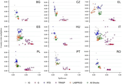
Figure 1 plots the country-wide multipliers against the spillovers for each region of a country, colour-coded by shock. The plots confirm that the most developed regions of the countries studied are generally characterised by smaller spillovers to other regions compared to the rest of the regions of a country. For certain shocks, investing in the most developed regions may be efficient, but not equitable: public investment, research and development and labour market shocks usually generate the highest country level returns but only a small portion spills outside the region. Transport infrastructure shocks often reveal that returns are higher in less developed regions which are also characterised by higher spillovers, and so investing there may be efficient and equitable at the same time, if most spillovers do not occur in the most developed region.

Figure 1. Country-wide multipliers and spillovers for each country (20 years), Armington elasticity = 4.

Note: X's represent the most developed region of each country colour-classified by type of shock. The six shocks are the following: Public current expenditure (G), public investment (IG), research and development (RTD), transport infrastructure investment (TRNSP), labour productivity (LABMKT) and all shocks; the simulations are performed for all the NUTS-2 regions of the nine countries of the sample.

Source: authors’ calculations. Nine country-specific scatterplots showing the relationship between country-wide multipliers and spillovers generated by region-specific shocks. The plotted points are colour-coded to show, separately, the different shocks.

The smaller spillovers generated by investing in the most developed regions are related to the consistently low intra-country import shares that these regions exhibit versus the rest of their countries. Table 3 shows that, on average, the most developed region imports 61% of its total imports from elsewhere in the respective country and the balance from abroad, while the complement regions import 72% on average, of which the majority originates in the most developed region. This explains the usually larger spillovers generated by investments in the less developed regions. This difference in trade flow intensity, together with the size of the share of the most developed region in the total spillover (shown in Table 2), are crucial for the results.⁶ Investment in the most developed regions leads to an increase in the demand for intermediate goods, a higher proportion of which comes from abroad than from within the country compared to other regions of the country, while the country-wide demand is met by a better reallocation of firms’ factors of production as capital and labour move to the most developed region and become part of the production process there.

Table 3. Intra-country import shares over total imports.

Most developed regions		Rest of the country
BG41, Yugozapaden*	54%	BG	74%
CZ01, Praha*	48%	CZ	65%
EL30, Attiki*	59%	EL	76%
ES30, Comunidad de Madrid*	78%	ES	79%
HU11, Budapest*	38%	HU	56%
ITC4, Lombardia	75%	IT	75%
PL91, Warszawski stołeczny*	78%	PL	77%
PT17, Área Metropolitana de Lisboa*	53%	PT	70%
RO32, Bucuresti – Ilfov*	64%	RO	77%

Note: Rest of the country import shares are the mean of a country’s regional import shares sans those of the most developed region. A ‘*’ denotes if the most developed region is also the capital city region. Source: authors’ calculations.

Table 4 summarises the cases of a trade-off between equity and efficiency for the three assumed values of the elasticity of substitution for each of the five simulated shocks, based on the results presented above. In most of the countries under analysis, the trade-off exists for investment in public infrastructure (IG), in labour market interventions leading to higher productivity (LABMKT) and in RTD interventions with consequences on TFP. On the other hand, shocks increasing public expenditure or improving transport infrastructures seem to be more likely to be both equitable and efficient, thanks to, on average, larger spillovers affecting, in a decisive way, the relationship between regional and country multipliers.

Table 4. Presence of an equity-efficiency trade-off, variation across three different values of the elasticity of substitution.

	Shocks
Country	G			IG			RTD			TRNSP			LABMKT
Trade elasticity	2	4	6	2	4	6	2	4	6	2	4	6	2	4	6
BG	No	No	No	Yes	Yes	Yes	Yes	Yes	Yes	No	No	No	Yes	Yes	Yes
CZ	No	No	No	Yes	Yes	Yes	Yes	Yes	Yes	Yes	Yes	Yes	Yes	Yes	Yes
EL	Yes	Yes	Yes	Yes	Yes	Yes	Yes	Yes	Yes	Yes	Yes	Yes	Yes	Yes	Yes
ES	No	No	No	No	Yes	Yes	No	Yes	Yes	Yes	Yes	Yes	Yes	Yes	Yes
HU	No	No	No	Yes	Yes	Yes	Yes	Yes	Yes	Yes	Yes	Yes	Yes	No	No
IT	No	No	No	No	No	No	No	No	No	No	No	No	Yes	Yes	Yes
PL	No	No	No	Yes	Yes	Yes	Yes	Yes	Yes	No	Yes	Yes	Yes	Yes	Yes
PT	No	No	No	Yes	Yes	Yes	Yes	Yes	Yes	Yes	Yes	Yes	Yes	Yes	Yes
RO	No	No	No	Yes	Yes	Yes	Yes	Yes	Yes	Yes	Yes	Yes	Yes	Yes	Yes

Note: G: public current expenditure. IG: public investment. RTD: research and development. TRNSP: transport infrastructure investment. LABMKT: labour productivity. Source: Authors’ calculations based on the 20-year country-wide multipliers.

Local conditions and initial stocks of labour, capital and intermediate production seem to be more important than local prices and trade, due to the stability in the results for different values of the trade elasticity. Nevertheless, it is interesting to look at the cases where the status of the trade-off changes when this parameter is modified. For example, in Spain, investments in public infrastructure (IG) and research and development (RTD) are equitable and efficient when regions trade in intermediate and/or final goods that are less substitutable with local goods (σ = 2), because the amount of spillovers generated in the less developed regions increases so much that they generate larger nationwide multipliers than those of the most developed region.

Identifying the conditions that are necessary for an equity-efficiency trade-off to emerge are not trivial, as location and initial conditions, the degree of substitutability and the intensity of interregional trade all matter. It should be examined whether investment in the most developed region enables growth in the less developed regions in a trickle-down fashion (Rauhut & Humer, 2020). Our results do not support trickle-down development from the core, as the nationwide returns to investment in the core are mostly realised in the region itself, and this effect dominates as the elasticity of substitution increases. Thus, cohesion funds allocation decisions should incorporate regional needs regarding the types of investment necessary as well as considerations on the potential effects on intra-country disparities.

5. CONCLUSIONS

We use a spatial dynamic general equilibrium model calibrated with data for all the NUTS-2 regions of the EU to simulate the macroeconomic impact of a suite of €100 million investments by activating both demand and supply channels within nine countries that are net recipients of cohesion policy funds. We combine the spatial economics and macroeconomics strands of the literature to analyse the interplay between region-specific and country-wide GDP impacts, paying particular attention to inter-regional spillovers within each country.

In regions characterised by a low intra-country import share, which is also where the concentration of production is high, the portion of returns generated elsewhere in the country, measured as spillovers, are found to be low. If overall country GDP impact is maximised by investing in such a region, then it can be claimed that for that particular type of investment, an equity-efficiency trade-off exists, since disparities with other regions of the country increase as returns, even though efficient, are highly localised. We find that this is mostly the case across countries for policy shocks that target public investments. To a lesser degree, an equity-efficiency trade-off is present in research and development, transport infrastructure, and labour productivity investments in Bulgaria, Czechia, Greece, Hungary, Spain, Poland, Portugal and Romania.

Relative to the argument of Rauhut and Humer (2020), that investment returns in the most developed regions of a country tend to propagate to other regions of the country and therefore should be used as a policy tool for investment activism, we find that this is not the case. The equity-efficiency trade-off dominates in regions with a high concentration of production and generate little spillovers elsewhere in a country. Such bundles of returns, even though they are efficient, amplify regional disparities. Investments that directly target the developing regions of a country, on the contrary, have the capacity to promote overall country growth and sometimes maximise it, while also reducing intra-country disparities.

Yet, both equity and efficiency of investments can co-exist, which depends on the combination of spillover strength and location, local returns on investment, and intra-country trade. These vary across countries and different types of investments, ultimately urging the policy-maker to consider regional needs when devising policy interventions capable of affecting economic growth and regional disparities. Future research could explore the question of the existence of a trade-off between equity and efficiency across EU countries. Finally, and as with any analysis based on economic modelling techniques, the results presented here are sensitive to a number of assumptions, so future research on this topic could explore alternative settings and modelling choices to assess the policy implications offered here, beyond the sensitivity checks already undertaken.

DISCLAIMER

The views expressed here are purely those of the authors and may not in any circumstances be regarded as stating an official position of the European Commission.

ACKNOWLEDGEMENTS

We thank the editor-in-chief, the guest editor, three anonymous reviewers, Patrizio Lecca, Damiaan Persyn, and the participants in the International Conference on Regional Science in Granada in October 2022 and in the Applied Economics Meeting in Toledo in June 2023 for valuable comments. All remaining errors are the authors’ own.

DISCLOSURE STATEMENT

No potential conflict of interest was reported by the author(s).

Correction Statement

This article has been corrected with minor changes. These changes do not impact the academic content of the article.

Notes

1 The model heavily borrows from economic geography, which, as Baldwin and Martin (2004) state, is at the crux of the trade-off between equity and efficiency. The literature offers a number of contributions on the existence of substantial spillovers generated by cohesion policy investigated using economic modelling methods (see, among others, Crucitti et al., 2023b; Pfeiffer et al., 2021; Blouri & Ehrlich, 2020; Varga and in’t Veld, 2011).

2 The methodology relies on a cost-benefit analysis based on Persyn et al. (2022) to select the roads to be upgraded for a given investment in a region. The approach starts by estimating the traffic volume on each road segment, taking into account regional trade flows between all EU regions. A gravity equation combined with geographic information is used to project the given trade data for each pair of regions onto the road network in order to impute the number of trucks on all road segments on the cheapest route connecting each sampled pair of regional centroids (several centroids are sampled for each region). The total gross economic gain from upgrading a road is then calculated by comparing the cost of traffic on a road with the hypothetical cost of traffic on the upgraded road. The gross gain is compared to an assumed construction cost (€5 million/km). This procedure identifies the road segments that would generate the largest economic gain if upgraded. All segments are ranked and it is assumed that improvements will be made to the roads with the largest benefits first, until the funds allocated to the region are exhausted (this does not happen with the €100 million shocks simulated here). These estimates rely only on road transport, which accounts for more than 75% of total freight transport in the EU (Eurostat, 2016). Nevertheless, we acknowledge this as a limitation and see it as an area of potential improvement for future analysis using this model.

3 Any choice of the size of the shock would be arbitrary and, given the non-linearity of the model, could lead to different results. However, firstly, we present the results for two different amounts (€100 million and €500 million); secondly, these amounts are comparable to the actual Cohesion Policy disbursements in the regions analysed; and thirdly, the use of multipliers reduces the concern with size in terms of comparability of results.

4 The observed multipliers are the product of the aggregate adjustments of the model’s variables in each period which lead to a change with respect to the baseline GDP value. For example, Figure A1 in Appendix 3 shows the yearly evolution of some key variables following a €500 million shock in BG31, Severozapaden, to show the macroeconomic implications of the shocks beyond the impact on GDP and its consequences on the equity-efficiency trade-off, which is the focus of the analysis.

5 Results for the 10- and 15-year outcomes of the simulations are presented in Tables A4 and A5 of Appendix 3 and show that there are no cases where the trade-off between equity and efficiency changes over time once the investments are fully deployed (which happens in the first 10 years of the simulation). Alternative results assuming a value of either two or six for the Armington elasticity are presented in Tables A6 and A7, respectively, in Appendix 4.

6 Note that the Armington trade elasticity affects the magnitude of the spillovers. As goods become more substitutable (i.e., the trade elasticity increases), the spillovers decline, with the largest changes observed outside the most developed regions. Region-specific multipliers increase, as regions reduce their reliance on intermediate goods imported from elsewhere. Table A8 in Appendix 4 shows that the relationship between the amount of the spillovers and the degree of substitutability is negative. In some cases the large size of the elasticity (six) causes the spillovers to be negative as factors of production move to the region receiving the investments, and the country wide multiplier becomes smaller than the region multiplier. We exclude these cases from our analysis and when calculating the percentage share of the impact occurring in the most developed region in Table 2. They are available in Tables A3 of Appendix 1, A6 and A7 of Appendix 4.

REFERENCES

- Allen, T., & Arkolakis, C. (2022). The welfare effects of transportation infrastructure improvements. The Review of Economic Studies, 89(6), 2911–2957. https://doi.org/10.1093/restud/rdac001
- Armington, P. S. (1969). A theory of demand for products distinguished by place of production. Staff Papers (International Monetary Fund), 16(1), 159–178. https://doi.org/10.2307/3866403
- Baldwin, R. E., & Martin, P. (2004). Agglomeration and regional growth. Handbook of Regional and Urban Economics, 4, 2671–2711. Elsevier. https://doi.org/10.1016/S1574-0080(04)80017-8
- Barbero, J., Christensen, M., Conte, A., Lecca, P., Rodríguez-Pose, A., & Salotti, S. (2023). Improving government quality in the regions of the EU and its system-wide benefits for cohesion policy. Journal of Common Market Studies, 61(1), 38–57. https://doi.org/10.1111/jcms.13337
- Barbero, J., Diukanova, O., Gianelle, C., Salotti, S., & Santoalha, A. (2022). Economic modelling to evaluate smart specialisation: An analysis of research and innovation targets in Southern Europe. Regional Studies, 56(9), 1496–1509. https://doi.org/10.1080/00343404.2021.1926959
- Barro, R. J. (1990). Government spending in a simple model of endogenous growth. Journal of Political Economy, 98(5), https://doi.org/10.1086/261726
- Battisti, M., & De Vaio, G. (2008). A spatially filtered mixture of β-convergence regressions for EU regions, 1980–2002. Empirical Economics, 34(1), 105–121. https://doi.org/10.1007/s00181-007-0168-8
- Baxter, M., & King, R. G. (1993). Fiscal policy in general equilibrium. American Economic Review, 83(3), 315–334. https://www.jstor.org/stable/2117521.
- Begg, I. (2016). The economic theory of cohesion policy. In Handbook on cohesion policy in the EU (pp. 50–64). Edward Elgar Publishing.
- Blouri, Y., & Ehrlich, M. V. (2020). On the optimal design of place-based policies: A structural evaluation of EU regional transfers. Journal of International Economics, 125, 103319. https://doi.org/10.1016/j.jinteco.2020.103319
- Bom, P. R. D., & Lightart, J. E. (2014). What have we learned from three decades of research on the productivity of public capital? Journal of Economic Surveys, 28(5), 889–916. https://doi.org/10.1111/joes.12037
- Bouayad-Agha, S., Turpin, N., & Védrine, L. (2013). Fostering the development of European regions: A spatial dynamic panel data analysis of the impact of cohesion policy. Regional Studies, 47(9), 1573–1593. https://doi.org/10.1080/00343404.2011.628930
- Breunig, R., & Rocaboy, Y. (2008). Per-capita public expenditures and population size: A non-parametric analysis using French data. Public Choice, 136(3), 429–445. https://doi.org/10.1007/s11127-008-9304-z
- Bronzini, R., & Piselli, P. (2009). Determinants of long-run regional productivity with geographical spillovers: The role of R&D, human capital and public infrastructure. Regional Science and Urban Economics, 39(2), 187–199. https://doi.org/10.1016/j.regsciurbeco.2008.07.002
- Card, D. (2001). Estimating the return to schooling: Progress on some persistent econometric problems. Econometrica, 69(5), 1127–1160. https://doi.org/10.1111/1468-0262.00237
- Castells, A., & Solé-Ollé, A. (2005). The regional allocation of infrastructure investment: The role of equity, efficiency and political factors. European Economic Review, 49(5), 1165–1205. https://doi.org/10.1016/j.euroecorev.2003.07.002
- Crucitti, F., Lazarou, N. J., Monfort, P., & Salotti, S. (2021). A scenario analysis of the 2021–2027 European cohesion policy in Bulgaria and its regions (No. 06/2021). JRC Working Papers on Territorial Modelling and Analysis, European Commission, Seville, JRC126268.
- Crucitti, F., Lazarou, N. J., Monfort, P., & Salotti, S. (2022). A cohesion policy analysis for Romania towards the 2021-2027 programming period (No. 06/2022). JRC Working Papers on Territorial Modelling and Analysis, European Commission, Seville, JRC129049.
- Crucitti, F., Lazarou, N. J., Monfort, P., & Salotti, S. (2023a). The impact of the 2014-20 European structural funds on territorial cohesion. Regional Studies, https://doi.org/10.1080/00343404.2023.2243989
- Crucitti, F., Lazarou, N. J., Monfort, P., & Salotti, S. (2023b). Where does the EU cohesion policy produce its benefits? A model analysis of the international spillovers generated by the policy. Economic Systems, 47(3), 101076. https://doi.org/10.1016/j.ecosys.2023.101076
- Edwards, J. H. Y. (1990). Congestion function specification and the ‘publicness’ of local public goods. Journal of Urban Economics, 27(1), 80–96. https://doi.org/10.1016/0094-1190(90)90026-J
- Eurostat. (2016). Road freight transport methodology. Eurostat.
- Farole, T., Rodríguez-Pose, A., & Storper, M. (2011). Cohesion policy in the European Union: Growth, geography, institutions. Journal of Common Market Studies, 49(5), 1089–1111. https://doi.org/10.1111/j.1468-5965.2010.02161.x
- Futagami, K., Morita, Y., & Shibata, A. (1993). Dynamic analysis of an endogenous growth model with public capital. Scandinavian Journal of Economics, 95(4), 607–625. https://doi.org/10.2307/3440914
- García-Rodríguez, A., Lazarou, N., Mandras, G., Salotti, S., Thissen, M., & Kalvelagen, E. (2023). A NUTS-2 European Union interregional system of Social Accounting Matrices for the year 2017: The RHOMOLO V4 dataset. JRC Working Papers on Territorial Modelling and Analysis No. 01/2023, European Commission, Seville, JRC132883.
- Glomm, G., & Ravikumar, B. (1994). Public investment in infrastructure in a simple growth model. Journal of Economic Dynamics and Control, 18(6), 1173–1187. https://doi.org/10.1016/0165-1889(94)90052-3
- Glomm, G., & Ravikumar, B. (1997). Productive government expenditures and long-run growth. Journal of Economic Dynamics and Control, 21(1), 183–204. https://doi.org/10.1016/0165-1889(95)00929-9
- Griffith, R., Redding, S., & Reenen, J. V. (2004). Mapping the two faces of R&D: Productivity growth in a panel of OECD industries. The Review of Economics and Statistics, 86(4), 883–895. https://doi.org/10.1162/0034653043125194
- Jorgenson, D. W., & Stephenson, J. A. (1969). Issues in the development of the neoclassical theory of investment behavior. The Review of Economics and Statistics, 51(3), 346–353. https://doi.org/10.2307/1926569
- Kancs, D., & Siliverstovs, B. (2016). R&D and non-linear productivity growth. Research Policy, 45(3), 634–646. https://doi.org/10.1016/j.respol.2015.12.001
- Krugman, P. (1991). Increasing returns and economic geography. Journal of Political Economy, 99(3), 483–499. https://doi.org/10.1086/261763
- Kyriacou, A. P., & Roca-Sagalés, O. (2012). The impact of EU structural funds on regional disparities within member states. Environment and Planning C: Government and Policy, 30(2), 267–281. https://doi.org/10.1068/c11140r
- Lecca, P., Christensen, M., Conte, A., Mandras, G., & Salotti, S. (2020). Upward pressure on wages and the interregional trade spillover effects under demand-side shocks. Papers in Regional Science, 99(1), 165–182. https://doi.org/10.1111/pirs.12472
- Männasoo, K., Hein, H., & Ruubel, R. (2018). The contributions of human capital, R&D spending and convergence to total factor productivity growth. Regional Studies, 52(12), 1598–1611. https://doi.org/10.1080/00343404.2018.1445848
- Mogila, Z., Miklosovic, T., Lichner, I., Radvanský, M., & Zaleski, J. (2022). Does cohesion policy help to combat intra-country regional disparities? A perspective on Central European countries. Regional Studies, 56(10), 1783–1795. https://doi.org/10.1080/00343404.2022.2037541
- Persyn, D., Barbero, J., Díaz-Lanchas, J., Lecca, P., Mandras, G., & Salotti, S. (2023). The ripple effects of large-scale transport infrastructure investment. Journal of Regional Science, 63(4), 755–792. https://doi.org/10.1111/jors.12639
- Persyn, D., Díaz-Lanchas, J., & Barbero, J. (2022). Estimating road transport costs between and within European Union regions. Transport Policy, 124, 33–42. https://doi.org/10.1016/j.tranpol.2020.04.006
- Pfeiffer, P., Varga, J., & in ‘t Veld, J. (2021). Quantifying spillovers of Next Generation EU investment. European Economy Discussion Papers no. 144, July 2021.
- Psacharopoulos, G., & Patrinos, H. A. (2018a). Returns to investment in education: A decennial review of the global literature. Education Economics, 26(5), 445–458. https://doi.org/10.1080/09645292.2018.1484426
- Psacharopoulos, G., & Patrinos, H. A. (2018b). Returns to investment in education: A decennial review of the global literature. World Bank Policy Working Paper No. 8402, Education Global Practice, World Bank Group, April 2018.
- Ramajo, J., Marquez, M. A., Hewings, G. J., & Salinas, M. M. (2008). Spatial heterogeneity and interregional spillovers in the European Union: Do cohesion policies encourage convergence across regions? European Economic Review, 52(3), 551–567. https://doi.org/10.1016/j.euroecorev.2007.05.006
- Rauhut, D., & Humer, A. (2020). EU cohesion policy and spatial economic growth: Trajectories in economic thought. European Planning Studies, 28(11), 2116–2133. https://doi.org/10.1080/09654313.2019.1709416
- Thissen, M., Ivanova, O., Mandras, G., & Husby, T. (2019). European NUTS-2 regions: Construction of interregional trade-linked supply and use tables with consistent transport flows. JRC Working Papers on Territorial Modelling and Analysis No. 01/2019, European Commission, Seville, JRC115439.
- Turnovsky, S. J. (1997). Fiscal policy in a growing economy with public capital. Macroeconomic Dynamics, 1(3), 615–639. https://doi.org/10.1017/S1365100597004045
- Varga, J., & in’t Veld, J. (2011). A model-based analysis of the impact of cohesion policy expenditure 2000–06: Simulations with the QUEST III endogenous R&D model. Economic Modelling, 28(1-2), 647–663. https://doi.org/10.1016/j.econmod.2010.06.004