How to control fluorescent labeling of metal oxide nanoparticles for artefact-free live cell microscopy

Abstract

Nanotechnologies hold great promise for various applications. To predict and guarantee the safety of novel nanomaterials, it is essential to understand their mechanism of action in an organism, causally connecting adverse outcomes with early molecular events. This is best investigated using noninvasive advanced optical methods, such as high-resolution live-cell fluorescence microscopy, which require stable labeling of nanoparticles with fluorescent dyes. However, as shown here, when the labeling is performed inadequately, unbound fluorescent dyes and inadvertently altered chemical and physical properties of the nanoparticles can result in experimental artefacts and erroneous conclusions. To prevent such unintentional errors, we introduce a tested minimal combination of experimental methods to enable artefact-free fluorescent labeling of metal-oxide nanoparticles—the largest subpopulation of nanoparticles by industrial production and applications—and demonstrate its application in the case of TiO₂ nanotubes. We (1) characterize potential changes of the nanoparticles’ surface charge and morphology that might occur during labeling by using zeta potential measurements and transmission electron microscopy, respectively, and (2) assess stable binding of the fluorescent dye to the nanoparticles with either fluorescence intensity measurements or fluorescence correlation spectroscopy, which ensures correct nanoparticle localization. Together, these steps warrant the reliability and reproducibility of advanced optical tracking, which is necessary to explore nanomaterials’ mechanism of action and will foster widespread and safe use of new nanomaterials.

Keywords:

• Dye leakage
• labeling characterization
• artefacts
• labeling-induced changes
• reliable nanomaterial labeling

1. Introduction

The rapid development of new materials is inevitably accompanied by their processing, combustion, and degradation, which can release particulate matter into the environment and increase our daily exposure to nanomaterials (Biswas and Wu 2005; Handy, Owen, and Valsami-Jones 2008; Klaine et al. 2008). This is further made worse by the wide use of nanomaterials in various industrial branches, including pharmacy (Senapati et al. 2018; Ziental et al. 2020) and the food industry (Lim, Bae, and Fong 2018; Chen et al. 2020)—all due to their unique properties. Consequently, there is a growing concern regarding the safety of nanomaterials, urging mandatory testing for their potential toxic effects (Gupta and Xie 2018; Baranowska-Wójcik et al. 2020). Sadly, it has been recognized that many nanomaterials interfere with classic cytotoxicity assays (Kroll et al. 2012), troubling their safety assessments and hence hindering their development.

To ease the introduction of safe nanomaterials into our daily lives, the scientific community has recognized the need for a deeper understanding of the link between adverse outcomes (nanoparticle toxicity) and nanoparticle characteristics (Nel et al. 2013; Murphy et al. 2015; Gerloff et al. 2017; Halappanavar et al. 2020). To unravel fundamental molecular mechanisms of nanoparticle toxicity, it is crucial to identify the involved molecular events and their causal relationships. However, nanoparticles are known to induce artefacts in several biochemical and spectroscopy-based assays because of their characteristic optical properties and affinity toward biomolecules (Kroll et al. 2012; Ong et al. 2014; Guadagnini et al. 2015), requiring the development and use of alternative experimental approaches.

One of the currently most powerful experimental techniques to study early molecular events is fluorescence microscopy—especially its advanced super-resolution implementation with spatial and temporal resolution on the order of tens of nanometers and seconds, respectively—which enables nanoparticle localization and monitoring of the complex network of interactions within and between living cells in real-time (Thurn et al. 2009; Kenesei et al. 2016; Urbančič et al. 2018; Chen et al. 2019; Kokot et al. 2020). However, since most of the nanoparticles are not intrinsically fluorescent, this experimental technique requires special preparation of the nanomaterial.

Here, we will focus on fluorescent labeling which binds fluorescent dyes to the nanoparticle. As most commercially available fluorescent dyes bind weakly to the native surface of the majority of nanoparticles, a commonly-used approach is to functionalize the nanoparticle surface with a coupling agent to create a link between the inorganic surface of the nanoparticle and the organic fluorescent molecule (Xia et al. 2008; Baumgärtel, Borczyskowski, and Graaf 2013; Garvas et al. 2015). Importantly, this enables fluorescent labeling of pre-synthesized and commercial nanoparticles with commercial fluorescent dyes, which are optimized for a specific microscopy technique. An alternative approach, luminescence labeling, can be utilized by doping the nanomaterial with lanthanides during its synthesis (Ranjit et al. 2001; Bettinelli et al. 2006), which increases the photostability of the labeled nanomaterial and minimizes the lanthanide dissolution. However, the multistep synthesis of the doped nanomaterial is lengthy, requires optimization for every dopant separately, yields less bright fluorescence, and, unfortunately, cannot be applied to already synthesized nanomaterials.

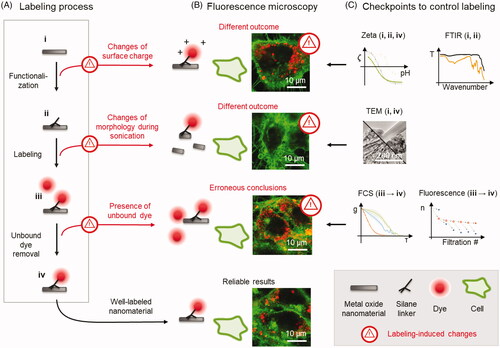
In order for our method to be applicable to the widest range of nanomaterials, the quality-controlled labeling procedure that is assessed here is designed in a way so it can be generalized to any functionalization of a nanomaterial with an appropriate linker, attachment of a fluorescent dye, and removal of the unbound dye (Figure 1(a)). Noteworthy, though, each of these steps can inadvertently change the properties of the nanomaterial, such as its morphology, surface charge, and the quantity of nonspecifically adhered dye (Pietzonka et al. 2002; Grafmueller et al. 2015), thereby also altering the nanoparticle’s interactions with the environment and hence affecting the interpretation of a fluorescence localization and tracking experiment (Figure 1(b)). Thus, reproducibility and reliability of experiments with fluorescent nanomaterial can be assured only if the labeling procedure of nanoparticles is carefully controlled at each step that can potentially alter the nanomaterial properties.

Figure 1. Overview of nanomaterial labeling with fluorescent dyes for live cell imaging, with checkpoints to prevent inadvertent changes to the original nanomaterial. (a) Schematic of nanomaterial labeling: the initial nanomaterial (i) is functionalized with a linker (ii), to which a fluorescent dye is bound (iii), and finally the unbound dye is washed away (iv). Note that the scheme elements are not drawn to scale. (b) Comparison of fluorescence micrographs of LA-4 cells (membranes labeled with CellMask Orange, shown in green) incubated with the exemplary nanomaterial—TiO₂ nanotubes—that were either adequately (bottom-most) or inadequately (top three images) fluorescently labeled with Alexa Fluor 647 (shown in red). Inadequate labeling results in different outcomes of the experiments and thus possibly leads to erroneous conclusions. For micrographs of separate color channels refer to Figure S1 in Supporting Information. (c) Proposed checkpoints to prevent such errors by measuring the nanomaterial properties at several stages during the labeling procedure.

Several cases of fluorescent labeling or doping of different nanoparticles, ranging from gold and metal oxides to carbonaceous and polystyrene nanoparticles, have been reported, with various degrees of quality control and nanomaterial characterization. To characterize the nanomaterial morphology, labeling protocols of nanoparticles are often paired with scanning- (SEM) and/or transmission-electron microscopy (TEM) of either the native surface before labeling (Sahoo et al. 2005; Xia et al. 2008; Garvas et al. 2015; Brown et al. 2018) or of labeled nanoparticles (Ge et al. 2009). When the dye is added during nanomaterial synthesis, often only the labeled nanomaterial is characterized (Pietzonka et al. 2002; Holzapfel et al. 2005; Jiang et al. 2011; Shang et al. 2012; 2014; Giordani et al. 2014; Grafmueller et al. 2015; Shahabi, Treccani, and Rezwan 2016). Importantly, one must be aware that the labeling procedures often involve vigorous sonication to disperse the nanomaterial, which can alter the morphology of nanoparticles (Hennrich et al. 2007), as shown in Figure 1.

Further surface modifications can arise from functionalization of the nanomaterial with a charged linker and fluorescent dye, which can alter the surface charge of the nanoparticles. This can be determined by Zeta potential measurements but is usually measured for either non-labeled or labeled nanoparticles (Holzapfel et al. 2005; Xia et al. 2008; Blumenfeld et al. 2014; Shahabi, Treccani, and Rezwan 2016). However, only the comparison of the two (Garvas et al. 2015) can give additional information on the success of the functionalization and labeling as well as possible labeling-induced modifications to the nanomaterial. Even more, the pH-dependence of the Zeta potential of any sample is rarely determined over the full pH range, yet only its full assessment (Shang et al. 2012; Garvas et al. 2015) would allow predicting the surface charge of the nanoparticles in various cellular compartments with varying pH—for instance, in the phagolysosome (Cho et al. 2012); such information can predictably impact the interpretation of experimental results. Besides Zeta potential, many other experimental methods can also test the success of the nanoparticle’ surface functionalization: Fourier transform infrared spectroscopy (FTIR) (Soares et al. 2006; Singh et al. 2008; Chen and Yakovlev 2010; Zhao et al. 2012; Killian 2013; Garvas et al. 2015), high angle annular dark-field scanning transmission electron microscopy (HAADF-STEM) (Garvas et al. 2015; Jiang et al. 2020), secondary ion mass spectrometry (SIMS) (Killian 2013), energy dispersive X-ray spectroscopy (EDX) (Killian 2013), and/or X-ray photoelectron spectroscopy (XPS) (Soares et al. 2006; Singh et al. 2008). Although crucial, such a step is often omitted.

With time and/or change of the environment of the labeled nanoparticles, the linker or the fluorescent dye may desorb from the nanoparticles, potentially leading to experimental artefacts due to the unbound dye being indistinguishable from labeled nanomaterial on fluorescence micrographs (Figure 1(b)) (Pietzonka et al. 2002; Tenuta et al. 2011; Grafmueller et al. 2015; Shahabi, Treccani, and Rezwan 2016). Various methods are useful to remove the free fluorescent dye, including dialysis (Tenuta et al. 2011; Garvas et al. 2015), gel filtration (Pietzonka et al. 2002), centrifugal filtration (Jiang et al. 2011; Shang et al. 2012; Urbančič et al. 2018), or a sequence of centrifugation and supernatant-removal (Xia et al. 2008; Giordani et al. 2014). The latter two methods enable precise characterization of free dye removal and dye desorption from the nanoparticles by analyzing filtrates or supernatants, respectively. In the other approaches mentioned, dye desorption must be tested in an additional separate step (Tenuta et al. 2011; Grafmueller et al. 2015; Shahabi, Treccani, and Rezwan 2016)—even for commercially available labeled particles (Schür et al. 2019).

To prevent erroneous conclusions from experiments performed with inadequately labeled and/or inadvertently changed nanomaterial, we propose and describe a minimal list of essential experimental checkpoints that ensure the labeling quality, characterize nanomaterial modification during labeling, and determine the rate of dye desorption (Figure 1(c)). These checkpoints should be measured at all major stages of the labeling procedure:

• i For native nanomaterial (Zeta potential, FTIR and TEM),

• ii For functionalized nanomaterial (Zeta potential and FTIR),

• iii → iv During free dye removal (FCS and fluorescence intensity), and

• iv For labeled nanomaterial (TEM and Zeta potential)

(See also the schematic in Figure S2 and flowchart in Figure S3 in Supporting Information).

We demonstrate their application of these checkpoints in the case of fluorescent labeling of TiO₂ nanotubes, highlighting possible consequences of skipping the checkpoints at each step. The exemplary nanomaterial was chosen from the class of TiO₂ nanoparticles, which are abundantly used in paints, sunscreens, pharmaceuticals, food additives, etc., and are as such often included in nanotoxicity studies. For reference, the step-by-step labeling protocol of the TiO₂ nanotubes is included in Supporting Information.

2. Results and discussion

2.1. Characterization of pristine material

Before the labeling process, pristine nanomaterial (i) must first be thoroughly characterized. Even if provided by the manufacturer, it is recommended to measure the nanoparticle’s specific surface, elemental composition, and structure, for example by using the BET method (Brunauer–Emmett–Teller method), EDXS (Energy-dispersive X-ray spectroscopy), and XRD (X-ray diffraction), respectively. It is also important to be aware of the method of nanomaterial synthesis and chemicals that were used during the process because these chemicals can incorporate into or adsorb to the nanomaterial, changing its properties. For our TiO₂ nanotubes, this has been extensively done and described previously (Garvas et al. 2015).

At this stage, it is also crucial to determine the morphology of the native material with TEM (transmission electron microscopy) and its surface properties by measuring the pH dependence of the Zeta potential over the entire pH range. As will be discussed later on, these results are compared with the material’s properties during and after labeling to characterize potential labeling-induced modifications of morphology and surface charge.

2.2. Functionalization of nanomaterial

Because fluorescent dyes do not bind covalently to the native surface of most metal oxides, the nanoparticles first need to be functionalized by binding a small linking chemical compound (linker) to the native nanoparticle surface (Figure 2(a), i → ii). The amount of linker used should enable efficient labeling (i.e., the labeled nanomaterial has enough dyes attached to be detected in the experiments) while minimizing changes to the native surface of nanomaterial. The step-by-step protocol for the functionalization of TiO₂ nanotubes with 3-(2- aminoethylamino)propyltrimethoxysilane (AEAPMS) is provided in the Supporting Information. Importantly, functionalization of various other metal oxide nanoparticles, the largest subpopulation of nanoparticles by industrial production and applications, can be achieved using a similar silane linker and procedure as described in this manuscript—e.g. functionalization of ZnO (Soares et al. 2006), TiO₂ (Zhao et al. 2012; Killian 2013)_, MgO (Killian 2013), ZrO₂ (Killian 2013) and metal oxide nanoparticles in general (LaGraff et al. 2003; Belmont and Cabot Corporation 2010; Mallakpour and Madani 2015).

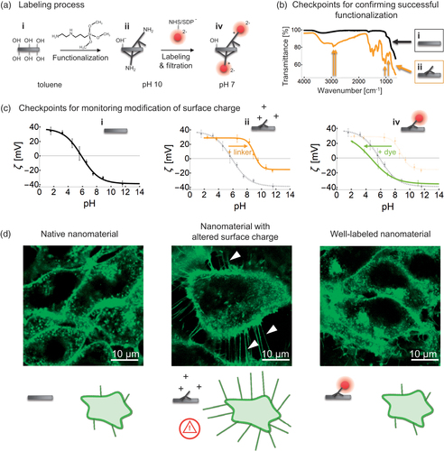
Figure 2. Functionalization and labeling of TiO₂ nanotubes with AEAPMS and Alexa Fluor dyes. (a) The schematics shows the chemical reactions taking place on the surface of nanotubes upon their functionalization and subsequent fluorescent labeling, highlighting the dissociating chemical groups and their charges. (b) An ATR-FTIR spectrum of pristine (shown in black, i) and successfully functionalized TiO₂ nanotubes (shown in brown, ii), with corresponding schematics of the samples. Brown arrows indicate vibration bands of the chemical bonds of the AEAPMS linker, attached to the TiO₂ surface (from left to right: C–H stretching, C–H stretching, Si–O–Si, and Ti–O–Si). Reference spectra of AEAPMS and solvents are shown in Figure S4, Supporting Information. (c) The pH-dependence of the Zeta potential (ζ) of i native TiO₂ nanotubes, ii functionalized nanotubes, and iv nanotubes labeled with Alexa Fluor 488. Arrows on the graphs indicate the shift in Zeta potential between different stages. (d) Comparison of confocal fluorescence micrographs of LA-4 epithelial cells (cell membranes are labeled with CellMask Orange and shown in green) after a 2-day exposure to (from left to right): unlabeled TiO₂ nanotubes, functionalized nanotubes with a more positive surface charge, and TiO₂ nanotubes labeled with Alexa Fluor 647, whose surface resembles the native nanotube (its fluorescence is not shown). The ratio between the surface of the nanotubes and surface of cells (so-called surface dose) was 10:1, 1:1, and 1:1, respectively. Notice the long filaments on the cell in the middle micrograph (arrowheads) which occur when the surface charge of the nanotubes is changed and are absent in the micrographs of both the native and well-labeled nanotubes.

When using a silane linker, in our case AEAPMS, the functionalization must be done in water-free toluene to prevent the formation of a water layer on the nanoparticle surface, which would disable the interaction between the linker and OH groups on the nanoparticles’ surface due to charge screening (Killian 2013), resulting in unsuccessful functionalization. The functionalized nanomaterial should be dried and stored as a powder to prevent desorption of the linker during storage.

2.2.1. Characterization of nanomaterial functionalization

The success of functionalization is assessed using attenuated total reflection Fourier-transform infrared spectroscopy (ATR-FTIR) of the native (i) and functionalized nanomaterial (ii). If the functionalization has been successful, the spectrum of the functionalized nanomaterial should contain not only the sum of the spectra of the linker and pristine nanomaterial, but also additional peaks, corresponding to the chemical bonds created by the binding of the linker to the nanomaterial (Garvas et al. 2015). As shown in Figure 2(b) for the pristine (shown in black) and successfully functionalized TiO₂ nanotubes (shown in brown), the presence of the AEAPMS linker on the washed functionalized nanotubes is confirmed by the presence of C-H stretching and Si-O-Si bonds in the spectrum (denoted by the three left-most arrows), whereas the binding of the linker to the nanotube is confirmed by the presence of the Ti-O-Si bond in the spectrum (right-most arrow, see also Figure S4, Supporting Information). For comparison, an ATR-FTIR spectrum of poorly functionalized TiO₂ nanotubes using the same AEAPMS linker is shown in Figure S4, Supporting Information, containing only very weak characteristic peaks corresponding to the linker and linker-to-nanotube bonds.

At this stage, the pH-dependence of the Zeta potential of the functionalized nanomaterial is measured again (Figure 2(c), ii). By comparing these pH dependencies to those obtained for the native nanomaterial (Figure 2(c), i), the effect of the linker on the nanomaterial surface charge is further analyzed. For example, successful functionalization with the AEAPMS linker, which contains amino groups, shifts the isoelectric point (value at which the Zeta potential equals 0 mV) toward higher pH values (Figure 2(c) ii, orange arrow). If none or only a small amount of the linker has attached to the nanomaterial, the Zeta potential would remain unchanged (Figure S17, Supporting Information).

Although using both FTIR and Zeta potential measurements may seem redundant, each of them brings important clues into the assessment of the labeling. On one hand, FTIR provides the required specificity in detecting the bond between the linker and the nanomaterial, while distinguishing unbound linkers from solvents and impurities. On the other hand, Zeta potential measurements of dispersed nanomaterial provide crucial information for choosing the appropriate charge of the fluorescent dye which shall counterbalance the potential charge effect of the linker to restore the surface charge of the labeled nanomaterial to the native value.

2.2.2. Potential artefacts

Importantly, the amount and charge of both the linker and the dye determine the final surface charge of the labeled nanomaterial, majorly influencing its interactions and mechanism of action in the cells and our bodies (Verma and Stellacci 2010; Zhu et al. 2013). An example of this is shown in Figure 2(d) for TiO₂ nanotubes with different surface charges. The morphology of the lung epithelial cells after a 2-day incubation with positively charged nanotubes is remarkably different than the morphology observed when they were incubated with native or labeled nanotubes, indicating an effect of modified surface charge on the cell response to the nanotubes. However, if the nanotubes’ Zeta potential was not determined before the measurement, these morphological changes and other toxicological outcomes could be wrongly attributed to the native nanotubes.

2.3. Fluorescent labeling

2.3.1. Selection of the fluorescent dye

After verifying the functionalization step, the nanomaterial is ready to be labeled with the desired fluorescent dye. The choice of the dye must adhere to several criteria, and may even affect the choice of the linker. In short, the dye should be capable of forming a covalent bond with the linker, be appropriately charged to allow the surface charge of the labeled material to be as close to native as possible, and have suitable characteristics for the planned optical experiments—all of which we discuss in detail below.

Regarding the binding chemistry, many commercial dyes are offered with various reactive groups: NHS (N-Hydroxysuccinimide) and SDP (sulfodichlorophenol) esters react with amines, maleimides react with thiol groups, hydrazides react with aldehydes and ketones, whereas azides and alkynes are used in ‘click’ reactions, to name a few.

The spectral characteristics of fluorophores must match the wavelengths of the excitation light, dichroic and emission filters of the fluorescence microscope on which the experiments are to be done (see example in Figure S5 in Supporting Information). Moreover, it is advised that their spectra are well separated from the spectra of other fluorophores that will be used simultaneously in the experiments to minimize cross-talk and bleed-through, which can give rise to false co-localization and misinterpretations if not appropriately corrected for (Demandolx and Davoust 1997; Zimmermann 2005; Gavrilovic and Wählby 2009). In live-cell applications, the dye should be bright and photo-stable to minimize the necessary excitation light flux, which can interfere with cellular processes during the experiment (Frigault et al. 2009). For use with advanced optical techniques (such as high-resolution microscopies, two-photon microscopy, fluorescence lifetime imaging, spectral imaging or correlation spectroscopy), further photo-physical aspects (e.g., lifetime, blinking, and environmental sensitivity) must also be taken into account.

Importantly, it is also necessary to select a dye which—in its unbound state—interacts with the sample as weakly as possible. Careful control of the number of dye molecules per nanomaterial can further decrease the interaction between the dye and the biological system. In general, it is always advisable to test the interaction between the dye and the sample with a control measurement, where the system is incubated with free dye instead of labeled nanomaterial for the desired amount of time (Zanetti-Domingues et al. 2013). By comparing the distribution and fluorescence intensity of the free dye with that of labeled nanomaterial, one can estimate the degree of false nanoparticle localization in the experiment (Schür et al. 2019).

Applying all these criteria to labeling of TiO₂ nanotubes, the dye should be an NHS or SDP ester for covalent binding to the primary amine NH₂ group (Banks and Paquette 1995) on the AEAPMS linker, and have a negative charge to compensate the positive charge of the linker. We further wanted the selected dye to be compatible with our high-resolution STED (stimulated emission depletion) microscope, for which bright and photo-stable far-red dyes work best. Also, interaction of the free dye with the system of interest needs to be taken into account: when unbound, the selected dye Alexa Fluor 647 does not stain the cell membrane due to a low membrane interaction factor—partially a consequence of its negative charge (Hughes, Rawle, and Boxer 2014)—and only a negligible fraction of the dye was localized in the cell after a 2-day incubation (Figure S6 Supporting Information).

2.3.2. Fluorescent labeling of nanomaterials

During the labeling step, when fluorescent dye is covalently bound to the linker on the nanomaterial (Figure 1 ii → iii), special care must be taken to ensure appropriate conditions for maximal labeling efficiency. Functionalized TiO₂ nanotubes and excess of fluorescent dye are combined according to the guidelines of the dye manufacturer. E.g., dyes with NHS and SDP esters must be stored in a water-free environment before labeling. For long-term storage the freshly opened dye is aliquoted in DMF (N,N-dimethylformamide), the DMF solvent is removed under high-vacuum (10 ⁻⁵bar) or lyophilization, and the aliquotes are stored under an inert gas (e.g. argon) at −70 °C. Just prior to labeling we dissolved the lyophilized probe in anhydrous DMSO (dimethyl sulfoxide).

Additional nanomaterial-specific requirements need to be considered: (1) To avoid nanoparticle aggregation during labeling, the concentration of nanoparticles should be kept below 1 mg/mL, the mixture should be sonicated by a tip sonicator while labeling, and the pH of the medium should be in the range where the nanoparticles are stable (the appropriate pH value can be deduced from the Zeta potential measurements from the previous step); (2) To improve the labeling efficiency, the linker and the fluorescent dye should be oppositely charged at the pH of the labeling medium, and the osmolarity of the labeling medium should be kept as low as possible to avoid charge screening.

2.3.3. Removal of the free and desorbed dye

Because the labeling is performed with an excess of fluorescent dye, the dye that did not bind to the nanomaterial must be removed before experiments to increase the contrast and avoid false localization of nanomaterial in fluorescence images. For the same reason, one also has to remove the dye that has desorbed from the fluorescently labeled nanomaterial during storage—typically due to desorption of the linker from the nanomaterial’s surface, not cleavage of the dye from the linker (Killian 2013). The free dye can be conveniently removed either with a sequence of centrifugations and supernatant removals, or using a centrifugal filter device that will let unbound dye pass through its filter. Both of these methods are quicker and use lower volumes of the washing media than the commonly used dialysis, enabling more reliable monitoring of the free dye removal due to higher concentrations of the dye in the filtrates (more on that below). It is also worth noting that this step removes any residual reagents from the functionalization and labeling, thus preventing their possible additional cytotoxic effects (Figure S9 in Supporting Information).

The first few filtrations should be made in a solvent in which the dye is soluble and nanomaterial is still well dispersed (in our case, a mixture of ethanol and diluted bicarbonate buffer in a 70:30 mass ratio, to achieve pH of 10, and osmolarity equivalent to 100-times diluted bicarbonate buffer, see Materials and methods section for details). The last few filtrations should use a medium that is not toxic to cells and in which the nanomaterial can be stably stored for extended periods of time (in our case, 100-times diluted bicarbonate buffer with pH 10) to remove the initial solvent. Also note that in-between centrifugations, the dispersion of nanoparticles should be gently sonicated on an ultrasound bath to minimize their aggregation and to desorb them from the filter or container.

2.3.4. Evaluation of labeling and free dye removal

The labeling efficiency, dye removal, and dye desorption from the nanomaterial can be evaluated either by fluorescence intensity measurements of the filtrates and retentates (i.e. remaining sample after filtration) or by fluorescence correlation spectroscopy (FCS) of the retentates, both of which we describe below; note that in the method using centrifugation and supernatant removal, supernatants correspond to filtrates and resuspended pellets to retentates. To this end, the FCS and fluorescence intensity measurements are more or less interchangeable; however, the equipment for fluorescence intensity measurements is more common than for FCS, which can, on the other hand, distinguish free dye from the dye bound to the nanoparticles in the same sample based on co-diffusion analysis. Hence, we usually use fluorescence intensity measurements during the filtration process and FCS for the final assessment of the labeled nanomaterial.

Evaluation by fluorescence intensity

The quantities of the dye in the filtrates and retentates after each filtration step are determined from the fluorescence intensity measurements, performed with a spectrophotometer, from which the absolute amounts (i.e., in moles) are calculated, taking into account the measured sample volumes, intensity-concentration calibration curves, scattering of light on the nanomaterial, as well as the influence of different media on the detected signal (see Figure S10–S14 in Supporting Information). The amount of the bound dye in the intermediate steps can be estimated from the fluorescence signal of the filtered dye (blue symbols in Figure 3(a)) to minimize the amount of the fluorescent material used for monitoring. In the estimations we neglected the losses of the dye stemming from its adsorption to the laboratory glassware and plastics, but nevertheless reached a good agreement with the actually measured values (in Figure 3(a), empty orange symbols extrapolate well toward the solid symbol); for more sticky dyes, though, additional calibration and correction may be required.

Figure 3. Removal of the free dye. (a) The strategy to control the removal of the free dye from the sample (TiO₂ nanotubes, labeled with Alexa Fluor 488) by centrifugal filtration relies on monitoring the quantity (n [nmol]) of the washed-away dye (blue markers) as well as the quantity of the dye remaining in the sample (orange markers, the values of empty ones were estimated as described in Supporting Information) for each consecutive step of filtration. (b) A control measurement of filtering only the free dye (Alexa Fluor 488) in the absence of nanotubes, performed in the same manner as in (a). (c) Normalized FCS curves (g(τ)) of TiO₂ nanotubes, labeled with Alexa Fluor 488, before filtration (red), after filtration (green), and with the same retentate measured after 14 days (blue). Note that the FCS curve of nanotubes before filtration (red) is almost undistinguishable from the curve of free dye (orange). (d) Comparison of confocal fluorescence micrographs of LA-4 cells (cell membranes labeled with CellMask Orange, shown in green) exposed to labeled TiO₂ nanotubes with various amounts of free dye in the sample (the bound and unbound dye is Alexa Fluor 647, shown in red and scaled so its fluorescence intensity is directly comparable across the images): a combination of labeled nanotubes and a 100-fold excess of free dye (300 nM), mimicking inefficient dye removal (left), cells exposed to correctly labeled and filtered nanotubes (approximately 3 nM of bound dye, middle), and cells exposed to free dye (1.6 nM, right). The ratio between the surface of the nanotubes and surface of cells is 1:1, 1:1 and 0:1 (from left to right). The localization of the fluorescent signal on the left two micrographs is very similar (arrowheads). For micrographs of separate color channels refer to Figure S8 in Supporting Information.

From the fluorescence signal of the final, cleaned retentate, we can estimate the degree of labeling of the nanomaterial. As a general guideline, the calculated number of dye molecules per nanoparticle should settle at a value above 1. In our case, the signal of the retentates settled at a value equivalent to the dye concentration of around 300 nM (orange symbols in Figure 3(a)), corresponding to 1.5 dye molecules per nanotube (calculations are discussed in Supporting Information). However, if the fluorescence of retentates does not settle (as demonstrated with filtration of free dye in Figure 3(b)), the dye did not bind to the nanomaterial, indicating that a change in the labeling strategy is required.

In an ideal case with no desorption of the dye from the nanoparticles, the filtrates’ signal should decrease exponentially with each subsequent filtration (Figure 3(b)). In a more realistic scenario (Figure 3(a)), however, the amount of the dye in the filtrates stabilizes after a few filtrations due to steady desorption of the dye from the nanotubes, with a lower value corresponding to more stable binding. Also, if the filtered sample is filtered again after a few days or weeks, the intensity of the first next filtrate will be higher than of the previous filtrate as it will contain all the dye that desorbed during this time period (Figure 3(a), filtrates #6 and #7). Note that measuring retentates at each step of filtration includes pipetting of small quantities of inhomogeneous nanomaterial suspensions, which can decrease the precision of determined amount of dye in the retentate (hence the difference between retentates #6 and #6 b in Figure 3(a)).

Evaluation by FCS

The nanoparticle labeling and free dye removal are additionally evaluated with fluorescence correlation spectroscopy (FCS) (Figure 3(c)) (Rigler and Meier 2006), which can distinguish free dye from the dye on the nanoparticles based on their diffusion properties, associated with their hydrodynamic radius. This can be determined via autocorrelated fluctuations of detected light, arising as the particles diffuse in and out of the observation volume (Magde, Elson, and Webb 1972; Elson 2011) (similarly as in dynamic light scattering (DLS), but relying on fluorescently emitted rather than scattered photons). As demonstrated in Figure 3(c), faster-diffusing, smaller entities with shorter transit times generate autocorrelation curves that are shifted toward shorter times (dotted curve, e.g. free dye) compared to larger, slower entities (dashed curve, e.g. dye on nanoparticles). From additional analysis of the autocorrelation curves and fluorescence fluctuations, one can also obtain the diffusion coefficient, hydrodynamic radius of the particles, their concentration, fraction of unbound dye, and number of dyes per nanoparticle (Rigler and Meier 2006). These parameters can be obtained for any freely-diffusing fluorescent entities, smaller than 10 μm—even for non-spherical nanoparticles, for which the calculated hydrodynamic radius is between the smallest and largest dimension of the nanomaterial, depending on the aspect ratio.

Note that FCS should be measured on retentates at a pH where the nanomaterial is stably dispersed. Otherwise, the light emitted from aggregates overwhelms the readouts of smaller diffusing molecules and nanoparticles, preventing the determination of diffusion properties of the latter. Importantly, such FCS measurements can be quickly performed even with a laser-scanning confocal fluorescence microscope just before an experiment to double-check the nanomaterial’s state (Nienhaus, Maffre, and Nienhaus 2013). As shown in Figure 3(c), the FCS curves of the non-filtered sample (red, iii) are dominated by the signal of the free dye (orange). In contrast, a well-filtered sample contains much slower diffusing entities (green, iv), indicating that most of the dye diffuses together with nanotubes. FCS curves of intermediate retentates, as well as of an old sample with some desorbed dye, show a weighted sum of these two extreme cases (blue, iv*), indicating the presence of both free and bound dye (see also Figure S15 in Supporting Information).

2.3.5. Potential artefacts

To resume, unbound dye in the sample can arise from the following:

• insufficiently removed unbound excess dye from the labeling step,

• desorbed dye that was adsorbed on the nanoparticle surface during the labeling step,

• desorbed linker with covalently bound dye.

All of these processes contribute to the false colocalization and misinterpretation of the measurements, when it is impossible to discern fluorescently labeled nanoparticles (Figure 3(d), middle) from large quantities of free dye (Figure 3(d), left).

Based on the fluorescence intensity and FCS checkpoint, the linker can be optimally selected to minimize desorption from the nanomaterial. This procedure has enabled us to identify the AEAPMS linker as the most suitable for reliable tracking of TiO₂ nanotubes. Its desorption was found to be relatively slow, and well-filtered samples were stable in the buffer for a few days (Figure 3(a)). If the nanomaterial has been stored for extended periods, we filter the nanomaterial at least once again before any cell-exposure experiments. Note that even if some of the dye desorbs from otherwise well-cleaned nanomaterial, its signal is homogeneously distributed over the large sample volume and therefore negligible (Figure 3(d), right) compared to the signal of a similar amount of the dye bound to the nanomaterial (Figure 3(d), middle). Also, in our case only a small fraction of the Alexa Fluor 647 dye was found internalized and localized in vesicles in the cells after a 2-day incubation (Figure S6 Supporting Information).

2.4. Characterization of labeled nanomaterial

Once the labeling is successfully performed, it must be verified that the labeled material preserved the desired properties of the native material, such as its native charge and morphology, which both knowingly affect interactions with cells (Verma and Stellacci 2010; Zhu et al. 2013; Vasile et al. 2015; Pujari-Palmer, Lu, and Ott 2017; Danielsen et al. 2020). Otherwise the functionalization and labeling procedure must be appropriately adjusted.

2.4.1. Potential artefacts due to altered charge

The final surface charge of the labeled nanomaterial is influenced by the amounts of bound linker and dye. Labeling the same functionalized nanomaterial at different conditions (dye concentration, timing, buffer etc.) can result in different pH-dependencies of Zeta potential (Figure S16 in Supporting Information), which can lead to different cellular response, as demonstrated before (Figure 2(d)). For cell exposure experiments, we therefore selected the labeled nanomaterial whose Zeta potential measurements were relatively close to those of the native nanomaterial (Figure 2(c), iv).

These measurements can also guide the optimization of the protocol: in our case, both the native and labeled TiO₂ nanotubes are stable in dispersion at pH 10 according to the measured Zeta potentials, so they are always sonicated and stored in 100-times diluted bicarbonate buffer with pH 10. The buffer is diluted to minimize screening of the charge on the nanotubes by ions in the buffer, thus enhancing the electrostatic repulsion and preventing aggregation of the nanotubes.

2.4.2. Potential artefacts due to altered morphology

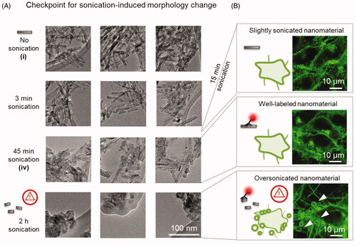
We next verified that the morphology of our TiO₂ nanotubes, determined from TEM measurements, remained similar to that of the native nanotubes (Figure 4(a), top three rows) despite the 45-minute sonication used in the labeling protocol, most of which is employed to increase labeling efficiency. However, longer sonication times markedly changed the morphology of the nanotubes (Figure 4(a), bottom). The TiO₂ nanotubes that were shorter due to a 2 hour sonication (Figure 4(b), bottom) also affected the cell’s morphology differently than nanotubes sonicated for 45 minutes (Figure 4(b), middle), which showed similar cellular response as non-labeled nanotubes sonicated for only 15 min (Figure 4(b), top). It is therefore essential to monitor for possible morphology changes of the nanomaterial, as they influence interactions with the cells and therefore the outcomes of cell-exposure experiments.

Figure 4. Inspection of the morphology of the nanomaterial to avoid sonication-induced modifications. (a) TEM images of (top to bottom) the initial TiO₂ nanotubes sample, and nanotubes sonicated for 3 min, 45 min and 2 h, with three sites per sample shown in columns. The delivered dose is 2 kJ per minute of sonication. The large flat structure in TEM images at 2 h sonication is a lacey carbon TEM grid. (b) Confocal fluorescent micrographs of cells (cell membranes are labeled with CellMask Orange and shown in green), exposed to TiO₂ nanotubes that were sonicated for 15 min (top), 45 min (middle) and 2 h (bottom) with the ratio between the surface of the nanotubes and surface of cells being 10:1, 1:1 and 1:1, respectively. The nanotubes in the lower two images are labeled with Alexa Fluor 647, the fluorescence of which is not shown. Note the vesicles and long filaments on the lowest micrographs (arrowheads) which are not observed in the other two micrographs.

2.4.3. Other potential artefacts due to sonication

It is also worth noting that many dispersion protocols use albumin or other proteins to improve the dispersion stability of nanomaterials. However, sonication may destabilize proteins and enhance their aggregation, which leads to the formation of biologically active, potentially immunogenic amyloid structures (Stathopulos et al. 2004). To exclude such effects, one could include a sham control to the experiments by sonicating the sonication medium without the nanoparticles and investigate its effects on the cells. If possible, however, a protocol for dispersing the nanomaterial without sonication of proteins is preferred.

Another often overlooked issue, related to tip-sonication of nanomaterials, is erosion of the transducer (tip) during sonication, which can contaminate the sample with metallic particles (Mawson et al. 2014), see also Figure S19 in Supporting Information. Tip erosion is increasingly prominent for longer sonication times, but can be mitigated by carefully polishing the tip and thoroughly washing it to remove debris from the polishing procedure. Tip polishing is best done between each of the subsequent sonications, or at the latest when a dark ring forms on the tip (Figure S19 in Supporting Information).

2.5. Examples of detection of early molecular events

After carefully following the labeling procedure with appropriate quality control steps, the well-characterized nanomaterial is ready for application in experiments. The rigorous evaluation of the material at all key preparation steps ensures minimal misinterpretation of the outcomes.

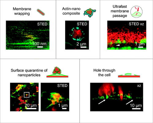
We exemplify the application of the resulting material in Figure 5, where cells have been incubated with TiO₂ nanotubes, labeled with Alexa Fluor 647, for 2 days before membrane staining and imaging. By using high-resolution fluorescence microscopy (stimulated emission depletion microscopy - STED), we were able to resolve a single nanotube inside the cell with a resolution well below the diffraction limit (Figure 5(c)). Co-localization of the fluorescence signal from the nanotube with the fluorescence from the membrane indicated that the nanotube was wrapped with the cellular membrane, as we reported previously (Urbančič et al. 2018). In our further studies, advanced fluorescence microscopy with well-labeled nanotubes enabled us to discover several novel events caused by interactions between the nanotubes and diverse cellular structures, such as membrane wrapping, formation of actin-nano composites, ultrafast passage of nanotubes through the plasma membrane, cell-induced quarantine of nanotubes on the cell surface, and formation of holes through the cell (Figure 6). Visualization and spatio-temporal characterization of such early molecular events allowed us to unravel causal relationships between them and understand their link to adverse outcomes after exposure to nanomaterials. In particular, we elucidated the mechanism how certain types of nanomaterials trigger previously unexplained chronic inflammation, based on which we designed an all-in-vitro test for its prediction (Kokot et al. 2020).

Figure 5. Super-resolution imaging of fluorescently labeled TiO₂ nanotubes in living cells. (a) The original STED image, and (b–d) corresponding zoom-ins, of LA-4 cells (membranes labeled with CellMask Orange, green) incubated for 2 days with efficiently and stably labeled nanotubes (Alexa Fluor 647, red), the ratio between the surface of the nanotubes and surface of cells being 1:1, as an example of an in vitro experiment. The signal of nanotubes is logarithmically scaled. For micrographs of separate color channels refer to Figure S20 in Supporting Information.

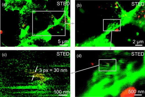
Figure 6. Examples of five early molecular events in living LA-4 cells following exposure to nanomaterial (TiO₂ nanotubes labeled with Alexa Fluor 647, red), detected with confocal or STED fluorescence microscopy. Cell membranes are labeled with CellMask Orange (green), actin with SiR Actin (cyan). For micrographs of separate color channels refer to Figure S21 in Supporting Information.

3. Conclusion

The use of fluorescently labeled nanomaterial in live-cell fluorescence microscopy requires stable and reliable binding of fluorescent dyes to the nanomaterial of interest, which, noteworthy, can modify nanomaterial properties and influence experimental results. Thus, to ensure the relevance and reproducibility of the experimental studies, it is of utmost importance to thoroughly characterize the labeled nanomaterial’s state and properties.

We here presented a procedure for quality control of nanoparticle labeling, which utilizes the following steps:

• Comparison of nanomaterial morphology before and after sonication by TEM: prolonged sonication can result in altered size/shape of the nanomaterial, causing it to interact differently with the cells than the native nanomaterial.

• Determination of the nanomaterial’s surface charge before and after labeling by measuring the pH-dependency of Zeta potential: both the linker and dye can influence the surface charge of the nanomaterial, affecting the response of cells as well.

• Removal of unbound dye by centrifugal filtration, monitored by intensity and FCS measurements: when free or desorbed dye is not sufficiently removed from the sample, the fluorescence signal can be falsely assigned to nanoparticles.

We illustrated the potential artefacts in cell-exposure experiments arising from missing out each step, and provided further practical advice on mitigating any issues should they arise. We here described the labeling process and demonstrated the application of the quality control procedure to TiO₂ nanotubes, functionalized with the AEAPMS silane linker and labeled with SDP-/NHS-esters of Alexa Fluor dyes. The described labeling procedure is suitable not only for the TiO₂ nanotubes, but for any nanomaterial that is capable of forming a stable bond with the silane linker—e.g. of ZnO (Soares et al. 2006), TiO₂ (Zhao et al. 2012; Killian 2013)_, MgO (Killian 2013), ZrO₂ (Killian 2013), and other metal oxide nanomaterials in general (LaGraff et al. 2003; Belmont and Cabot Corporation 2010; Mallakpour and Madani 2015). More importantly, the described quality control procedure can be directly applied to ensure reliable labeling of any nanoparticles and colloidal particles of up to 10 µm in size, above which the Zeta potential and fluorescence correlation spectroscopy experiments become unreliable.

By carefully monitoring the entire labeling procedure, identifying and troubleshooting unsuccessful labeling is significantly simplified. Moreover, the suggested procedure results in well-characterized and stably labeled nanomaterial that reproduces the pristine material’s mode-of-action, thus enabling reproducible, relevant and reliable nanotoxicity studies with advanced microscopies in live cells. These can uniquely identify and connect key molecular events that trigger adverse outcomes, which can lead toward better mechanistic understanding of nanoparticles’ effects on our health, design of more efficient testing strategies, and finally, safer use of the impressive technologies the nanomaterials can offer.

4. Experimental methods

Materials

Alexa Fluor 488 SDP ester (Thermo Fisher), Alexa Fluor 647 NHS ester (Thermo Fisher), CellMask Orange (Invitrogen), LCIS - Live Cell Imaging Solution (Invitrogen), #1.5H µ-dishes (Ibidi), PBS—phosphate buffer saline (Gibco), 100x dcb: 100-times diluted bicarbonate buffer (pH 10, osmolarity 5 mOsm L ^{− 1}, mixed in-house), F-12K cell culture medium (Gibco), Trypsin (Sigma), FBS (Fetal bovine serum, ATCC), Penicillin-Streptomycin (Sigma), Non-essential amino acids (Gibco), BSA-bovine serum albumin (Sigma), 3-(2- aminoethylamino)propyltrimethoxysilane (AEAPMS, Alfa Aesar), lacy carbon film supported by a 300-mesh copper grid (Ted Pella, Inc.), sodium bicarbonate buffer mixed in-house from NaHCO3 (Merck) and Na2CO3 (Kemika), anhydrous DMSO (Sigma Aldrich), ethanol (Carlo Erba), centrifugal filter device Amicon Ultra 4 mL 100 K (Merck Millipore), HCl (Merck), KOH (Sigma Aldrich), KCL (Merck), polystyrene cuvettes for Zeta potential measurements (Sarstedt), 96-well black flat-bottom microplate (Brand).

Software

Imspector (version 16.3.11462-win64) software provided by Abberior, SymPhoTime64 (PicoQuant), Mathematica 12.0 - license L5063-5112 (Wolfram).

TiO₂ nanotubes synthesis

TiO₂ nanotubes were synthesized in-house using the method, described elsewhere (Umek et al. 2005; Garvas et al. 2015). Synthesis of the anatase TiO₂ nanotubes with a diameter of 10 nm, mean length of 200 nm and a BET surface of 150 m² g⁻¹ proceeds in several stages:

• 1). Synthesis of sodium titanate nanotubes (NaTiNTs); $${\text{TiO}}_2+\mathrm{ }\text{NaOH}\left(\text{aq}\right)\mathrm{ }\to \mathrm{ }{\left(\text{Na},\mathrm{H}\right)}_2{\text{Ti}}_3{\mathrm{O}}_7{\text{xH}}_2\mathrm{O}$$

NaTiNTs are synthesized according to the method already reported elsewhere (Umek et al. 2007). In short, a suspension of TiO₂ (Titanium(IV) dioxide, anatase, 325 mesh, Aldrich) and 10 M NaOH (1 g TiO₂ per 10 mL 10 M NaOH) is ultrasonicated for 30 min and then stirred for 1 hour at room temperature. The suspension is transferred to a Teflon-lined autoclave; the filling volume is 80%. The closed autoclave is heated for three days at 135 °C. When the reaction mixture is cooled down to room temperature, the resulting material is washed twice with deionized water (2 × 300 mL), once with ethanol, and dried overnight at 100 °C. At this stage morphology is checked with scanning electron microscope (SEM).

• 2). Transformation of sodium titanate nanotubes to hydrogen titanate nanotubes (H₂Ti₃O₇); $${\left(\text{Na},\mathrm{H}\right)}_2{\text{Ti}}_3{\mathrm{O}}_7\to {\text{H}}_2{\text{Ti}}_3{\mathrm{O}}_7{\text{xH}}_2\mathrm{O}$$

Next, sodium ions are removed by an ion-exchange process; 2.5 g of sodium titanate nanotubes is dispersed into 300 mL of 0.1 M HCl(aq) (Umek et al. 2014). The prepared dispersion is stirred at room temperature for 1 h and centrifuged to separate the solid material from the solution. The dispersing, centrifuging and separating steps are repeated for three more times. At the end, the solid material is washed three times with 200 mL of distilled water and once with 100 mL of ethanol and dried overnight at 100 °C. At this stage the content of sodium and chlorine is determined with energy-dispersive X-ray spectroscopy (EDXS). If the content of sodium and/or chlorine is above 0.3 wt. % the washing procedure with 0.1 M HCl and deionized water was repeated.

• 3). Transformation of hydrogen titanate nanotubes to TiO₂ nanotubes; $${\text{H}}_{\text{2}}{\text{Ti}}_{\text{3}}{\text{O}}_{\text{7}}{\text{xH}}_{\text{2}}\text{O}\to {\text{TiO}}_{\text{2}}+{\text{H}}_{\text{2}}\text{O}$$

Finally, hydrogen titanate nanotubes are transformed to TiO₂ nanotubes by thermal treatment in air. In general, 500 mg of H₂Ti₃O₇ nanotubes is weighed in an alumina boat, placed into an oven and heated at a ramp rate of 1 °C min⁻¹ to 380 °C (or 400 °C). The sample is kept at 380 °C for 6 h, and cooled down to room temperature afterwards (Garvas et al. 2015). At this stage morphology is checked with SEM and TEM, structural analysis with XRD (X-ray powder diffraction), elemental composition with EDXS (Energy-dispersive X-ray spectroscopy) and specific surface with BET (Brunauer–Emmett–Teller method).

TiO₂ nanotubes functionalization (f-TiO₂)

TiO₂ nanotubes (100 mg) are dispersed sonically in 30 mL of dry toluen and then heated to 60 °C while constantly stirring. Separately, a solution of 840 µL of 3-(2-aminoethylamino)propyltrimethoxysilane (AEAPMS, Figure S22 in Supporting Information) in 30 mL of dry toluene is prepared. The solution of AEAPMS in toluene is added dropwise (30 minutes) to the dispersion of TiO₂ nanotubes in toluene. After 16 h the reaction mixture is cooled to room temperature and the solid material is separated from the liquid phase by centrifugation. Then, it is rinsed first with 30 mL of toluene (3 times) and then with 30 mL of hexane (3 times). The isolated product is dried overnight at 80 °C and for 2 hours at a vacuum drier at 80 °C and 150 mbars. The quality of functionalization is checked with FTIR and Zeta potential measurements. A step-by-step protocol for the functionalization is described in the Supporting Information.

TiO₂ nanotubes labeling

All labeling quantities refer to labeling of 1 mg of TiO₂ nanotubes, functionalized with AEAPMS (f-TiO₂), a linker with a positive charge at labeling pH. First, 1 mg of functionalized TiO₂ is weighed (Excellence Plus, Mettler Toledo) and diluted in 1 mL of 100-times diluted sodium bicarbonate buffer with pH = 10.00, which has been prepared in a glass flat bottom flask with fresh miliQ water. The sample is transferred to a glass vial. The Nanotubes are then sonicated with a tip sonicator (MISONIX Ultrasound Liquid Processor with 419 MicrotipTM), with the average power 35 W (amplitude set to 70) and a microtip with radius of 3 mm with a surface of 30 mm² for t_run = 15 min, t_on = 5 s, t_off = 5 s. This totals the sonication time to t = 15 min and total sonication dose 32 kJ.

After the first sonication, 3.2 μL of 12.1 mM fresh, negatively-charged Alexa Fluor 488 SPD ester or Alexa Fluor 647 NHS ester (Life Technologies, Figure S22 in Supporting Information), diluted in anhydrous DMSO, is added. For each mg of nanotubes, 40 nmol of label is added. Again, the sonication is performed with a tip sonicator for t_run = 30 min, t_on = 5 s, t_off = 5 s with total sonication dose 63 kJ. This totals the cumulative sonication time to t = 45 min and total sonication dose of 95 kJ. Note that the sonication dose at which the nanomaterial morphology remains unaltered needs to be verified for each nanomaterial separately.

After the sonication is complete, a mixing magnet is added to the glass vial containing the sample and is left to stir overnight on a magnetic mixer at 260 rpm, covered with aluminum foil to prevent photo-bleaching of the dye. After approximately 12–16 h of incubation, the magnet is removed from the glass vial. The sample is then centrifuged to remove excess unbound label. A detailed protocol for the labeling is described in the Supporting Information.

Free dye removal

The free dye is removed by centrifugation in a centrifugal filter device (CFD), which forces the sample through a filter during centrifugation, separating the sample into the filtrate below the filter (containing unbound dye) and retentate on the filter (containing nanoparticles, which are too large to pass through the filter), which is then resuspended. To ensure efficient filtration, the size of pores on the filter of the centrifugal device should be significantly larger than the fluorescent dyes and smaller than the nanoparticles.

Centrifugation is performed in a centrifuge filter device (CFD) (Amicon Ultra 4 mL 100 K) with a 100 kDa membrane with a centrifuge (LC-320, Tehtnica, Zelezniki) to achieve 1000 g. Firstly, the CFD is prepared for use according to the manufacturer’s guidelines, i.e. by centrifuging 2 mL of deionized water through the membrane. Then, 1 mL of labeled TiO₂ nanotubes are pipetted into the CFD and spun for 15 min. Afterwards, the filtrate is stored for further analysis and the retentate is resuspended (by mixing with a pipette) in 1 mL of medium, consisting of 70% ethanol and 100-times diluted bicarbonate buffer (39.37 mL of 96% ethanol is mixed with 0.5 mL non-diluted bicarbonate buffer and 11.27 mL of deionized water). The empty filtrate compartment is filled with the same medium so the membrane is submerged (this is to ensure good contact in the ultrasonic bath in the next step). The CFD is sonicated on the ultrasound bath (Branson 2510) for 20 s to diminish the amount of nanoparticles stuck to the CFD membrane and to break up the nanoparticle aggregates. The filtrate compartment is washed with ethanol and dried to prevent cross-contamination of subsequent filtrates, and the sample in the CFD is spun again.

The sample is filtered twice in this manner and two times more with 100-times diluted bicarbonate buffer as medium instead of the mixture of 70% ethanol and 100-times diluted bicarbonate buffer to reduce the amount of ethanol in the sample. As a general guideline, the filtered sample should have a noticeable color at 1 mg/mL, as should the very first filtrate and the color should decrease in subsequent filtrates (Figures S23 and S24, Supporting Information). It is also worth noting that a general idea of the cleaning efficiency can already be obtained by measuring the original sample, final cleaned sample and last filtrate (or, even better, two last filtrates). The sample should be filtered at least once more just prior to the experiments in the desired media, if it was stored in a refrigerator for longer periods of time (in our case more than two weeks). A more detailed protocol for the filtration process is described in the Supporting Information.

TEM and FTIR

The morphology of the nanotubes was investigated with a transmission electron microscope (TEM Jeol 2100, 200 keV). Specimens of nanotubes were dispersed ultrasonically in methanol and a drop of the dispersion was deposited onto a lacy carbon film supported by a 300-mesh copper grid. Infrared spectra were obtained via Attenuated total reflection Fourier transform infrared spectroscopy (ATR-FTIR) with a universal ATR accessory on a Spectrum 400 FTIR spectrometer (Perkin Elmer). The spectra were recorded with the resolution of 4 cm⁻¹ and 16 scans.

Zeta potential measurements

Zeta potential measurements were performed on NanoBrook ZetaPALS Potential Analyzer (Brookhaven) and electrode for non-organic solvents (AQ-1203, Brookhaven). For measurement of each part of the Zeta potential—acid and base—3 mL of sample diluted to c = 0.1 mg mL⁻¹ in 10 mM KCl was used. The pH was measured with a pH meter (Seven Multi, Mettler Toledo) and a 1 mm thick pH electrode (Inlab ExpertPro, Mettler Toledo) right before every measurement of the Zeta potential. Each of the 10 measurements at each pH value was measured until the experimental fit errors (residuals) were below the set value of 0.025. From the 10 measurements, the average and error were calculated.

The change of pH was achieved by addition of HCl (to lower pH) or KOH (to rise pH). After each addition, the sample was left on a magnetic stirrer (IKA topolino) for approximately 3–5 min or until stabilization of pH occurred.

Fluorescence intensity of filtrates

Free dye concentration measurements were performed on the spectrometer Tecan Infinite M1000 (Tecan Group Ltd., Männedorf, Switzerland). Samples have been loaded to 96-well plates (96-well plate, Brand) prior to the measurements in volumes of 150 μL. The amount of dye in the sample was calculated from the known volumes and concentrations, which were calculated from the measured fluorescent signal and previously measured calibration curves for concentration, medium and nanomaterial concentration in the sample. Direct comparison between samples was possible since all experimental conditions were the same (volume of sample, temperature, machine settings, etc.).

The filtrates were measured as-is, whereas a fraction of each retentate was taken away after the filtration and diluted to achieve the 150 μL needed for the fluorescence measurement in order to not use too much of the valuable labeled nanomaterial. For the same reason, fluorescence of intermediate retentates was estimated from the measured intensities of filtrates and other retentates (open circles in Figure 3(a)). Due to variations in filtration volumes, we calculated the absolute quantities of dye in the whole sample including the retentates used for measurements. A more detailed description is located in the Supporting Information.

Cell culture and sample preparation for microscopy

All fluorescence microscopy was done on LA-4 murine lung epithelial cells which were cultured according to ATCC guidelines: they were grown in a mixture of F-12K medium (Gibco), 15% FBS (Fetal bovine serum, ATCC), 1% P/S (Penicillin-Streptomycin, Sigma), 1% NEAA (non-essential amino acids, Gibco) in an incubator at 37 °C, saturated humidity and 5% CO₂. After incubation with nanotubes, the culture conditions remained the same.

For the fluorescence image comparison in Figures 1–4, the LA-4 cells were seeded in a 1.5H Ibidi µ-dish at 30% confluency. Two days later, the appropriate sample of nanotubes was added to the cells. For ‘well-labeled nanomaterial’ (Figure 2(d) right, Figure 3(d) middle, and Figure 4(b) middle), 35 µL of 0.1 mg mL⁻¹ TiO₂ nanotubes fluorescently labeled with Alexa Fluor 647 in PBS (phosphate-buffered saline) were added to 315 µL of full cell medium on cells to achieve a 1:1 ratio between the surface of the nanotubes and surface of cells (so-called surface dose). For sample preparation of other, incorrectly labeled nanotubes, see below. After 2 days of incubation with the nanotubes, the medium with cells was removed and cells were labeled with 100 µL of 5 µg mL⁻¹ CellMask Orange in Live Cell Imaging Solution (LCIS, Molecular Probes) for 6 min at 37 °C. Later, the medium with CellMask Orange was slowly removed and cells were observed in 100 µL LCIS.

The ‘native nanomaterial’ in Figure 2(d) (left) was incubated with a 10:1 surface dose of nonlabeled nanomaterial, the ‘nanomaterial with different surface charge’ in Figure 2(d) (middle) was incubated with a 1:1 surface dose of functionalized TiO₂ nanotubes. The ‘desorbed fluorophores’ in Figure 3(d) (right) was incubated with a 1.6 nM concentration of free Alexa Fluor 647, the ‘unwashed label’ in Figure 3(d) (left) was incubated with a mixture of 1:1 surface dose of well-labeled TiO₂-Alexa647 and free Alexa Fluor 647 to achieve a 3 nM final concentration of Alexa Fluor 647 on the nanotubes and an additional 300 nM concentration of unbound Alexa Fluor 647, mimicking insufficient filtration. The ‘slightly sonicated nanomaterial’ shown in Figure 4(b) (above) was sonicated for 15 minutes and exposed to the cells at a 10:1 surface dose, and the ‘oversonicated’ nanomaterial shown in Figure 4(b) (below) was sonicated for 2 h instead of 45 min during the labeling procedure and exposed to the cells at a 1:1 surface dose.

For the high-resolution STED image, the LA-4 murine lung epithelial cells were seeded into a 1.5H Ibidi µ-Dish at 30% confluency and cultured in complete medium. A 100 µg mL⁻¹ dispersion of TiO₂ nanotubes labeled with Alexa Fluor 647 in PBS was diluted in 270 µL of full cell medium to achieve the final concentration of 10 µg mL⁻¹. When added to the cells, this corresponded to a surface dose of 1:1. After 2 days of incubation, the samples were washed and the plasma membranes were labeled with 100 µl of 5 µg mL⁻¹ CellMask Orange in PBS. The sample was washed with PBS after 20 minutes of incubation and observed in PBS right afterwards. Larger confocal fields of view can be found in Figure S25 in Supporting Information.

FCS

For Fluorescence Correlation Spectroscopy (FCS), a PicoQuant MicroTime 200 confocal microscope was used. An Olympus IX81 inverted microscope was equipped with a 60× water immersion objective (Olympus UPLSAPO 60 × W NA1.2). Alexa Fluor 488 was excited by a pulsed laser of wavelength 488 nm (PicoQuant, Germany), at 40 MHz repetition rate and average power of about 5 μW at the objective. Fluorescence of the dye was acquired through a 531/40 emission filter (Brightline, Semrock) by an APD detector (tau-SPAD, PicoQuant, Germany), connected to a PicoQuant HydraHarp 400 single-photon-counting unit. Typical acquisition times were 5–15 min. The fluorescence fluctuations were analyzed using SymPhoTime64 (PicoQuant). For presentation, FCS curves were normalized to ease the comparison of their relative shapes.

Fluorescence microscopy and STED

The imaging was performed with an Abberior Instruments STED microscope using a 60x water immersion objective (Olympus UPLSAPO 60xW NA1.2) and the accompanying software Imspector (version 16.3.11462-win64). The fluorescence of CellMask Orange and TiO₂-Alexa647 was excited using two pulsed lasers at 561 and 640 nm, and their fluorescence was detected by two avalanche photodiodes at 580–630 nm and 650–720 nm (filters by Semrock), respectively. The confocal fluorescence images in Figures 1–4 were acquired using a pixel size of 100 nm, dwell-time 10 µs, and laser powers at around 20 µW.

The STED image in Figure 5 was acquired using a 10-nm pixel size. The resolution was increased by stimulated depletion of fluorescence by an 70 mW doughnut-shaped STED laser beam at 775 nm.

All experiments were performed at room temperature.

Associated content

Supporting Information Available: Supporting Information includes separate channels of fluorescence micrographs, additional supporting schemes, measurements and calculations, and a detailed step-by-step protocol for labeling TiO₂ nanotubes as described in the manuscript (PDF).

Author contributions

The manuscript was written through contributions of all authors. All authors have given approval to the final version of the manuscript. ‡BK and HK contributed equally as first authors. # TK, IU and JŠ contributed equally as corresponding authors.

BK, HK, PU, SP, MG, CE, TK, IU, JŠ designed the study and analysis.

PU synthesized the nanotubes.

PU and SP functionalized the nanotubes.

BK, HK, KPvM labeled the nanotubes.

BK, HK, PU, KPvM, IU prepared the samples.

BK, HK, PU, IU performed the experiments.

BK, HK, IU analyzed the data.

CE, TK, IU, JŠ supervised the study.

BK, HK prepared the manuscript with input from all other authors: PU, KPvM, SP, MG, CE, TK, IU, JŠ.

Acknowledgment

The authors thank Monika Koren, Neža Golmajer Zima, Petra Čotar and David Dolhar for their help with the preparation of samples, Aleksandar Sebastijanović for kindly providing the micrograph of actin-nano composite as well as drs. Silvia Galiani and Falk Schneider for their help with the FCS experiments.

Disclosure statement

No potential conflict of interest was reported by the author(s).

Data availability statement

Data is available from authors upon reasonable request.

Additional information

Funding

This research was funded by EU Horizon2020 Grant No. 686098 (SmartNanoTox project), Slovenian Research Agency [program P1-0060], Young Researcher Program [PR-08331, H. Kokot], Marie Skłodowska-Curie Individual Fellowship [grant no. 707348 to I. Urbančič], and Wolfson Foundation/Medical Research Council [MRC, grant no. MC_UU_12010/unit programmes G0902418 and MC_UU_12025]/Deutsche Forschungsgemeinschaft (Jena Excellence Cluster ‘Balance of the Microverse’, Collaborative Research Center 1278 ‘Polytarget’) to C. Eggeling.

References

- Banks, P. R., and D. M. Paquette. 1995. “Comparison of Three Common Amine Reactive Fluorescent Probes Used for Conjugation to Biomolecules by Capillary Zone Electrophoresis.” Bioconjugate Chemistry 6 (4): 447–458. doi:https://doi.org/10.1021/bc00034a015.
- Baranowska-Wójcik, E., D. Szwajgier, P. Oleszczuk, and A. Winiarska-Mieczan. 2020. “Effects of Titanium Dioxide Nanoparticles Exposure on Human Health-a Review.” Biological Trace Element Research 193 (1): 118–129. doi:https://doi.org/10.1007/s12011-019-01706-6.
- Baumgärtel, T., C. von Borczyskowski, and H. Graaf. 2013. “Selective Surface Modification of Lithographic Silicon Oxide Nanostructures by Organofunctional Silanes.” Beilstein Journal of Nanotechnology 4 (1): 218–226. doi:https://doi.org/10.3762/bjnano.4.22.
- Belmont, J. A., and Cabot Corporation. 2010. Compositions comprising silane modified metal oxides. US Patent No. US9382450 B2. http://patents.google.com/patent/US9382450.
- Bettinelli, M., A. Speghini, D. Falcomer, M. Daldosso, V. Dallacasa, and L. Romanò. 2006. “Photocatalytic, Spectroscopic and Transport Properties of Lanthanide-Doped TiO2 Nanocrystals.” Journal of Physics: Condensed Matter 18 (33): S2149–S2160. doi:https://doi.org/10.1088/0953-8984/18/33/S30.
- Biswas, P., and C.-Y. Wu. 2005. “Nanoparticles and the Environment.” Journal of the Air & Waste Management Association (1995) 55 (6): 708–746. doi:https://doi.org/10.1080/10473289.2005.10464656.
- Blumenfeld, C. M., B. F. Sadtler, G. E. Fernandez, L. Dara, C. Nguyen, F. Alonso-Valenteen, L. Medina-Kauwe, et al. 2014. “Cellular Uptake and Cytotoxicity of a Near-IR Fluorescent Corrole-TiO2 Nanoconjugate.” Journal of Inorganic Biochemistry 140: 39–44. doi:https://doi.org/10.1016/j.jinorgbio.2014.06.015.
- Brown, K., T. Thurn, L. Xin, W. Liu, R. Bazak, S. Chen, B. Lai, et al. 2018. “Intracellular in Situ Labeling of TiO2 Nanoparticles for Fluorescence Microscopy Detection.” Nano Research 11 (1): 464–476. doi:https://doi.org/10.1007/s12274-017-1654-8.
- Chen, Q., and N. L. Yakovlev. 2010. “Adsorption and Interaction of Organosilanes on TiO2 Nanoparticles.” Applied Surface Science 257 (5): 1395–1400. doi:https://doi.org/10.1016/j.apsusc.2010.08.036.
- Chen, S., J. Wang, B. Xin, Y. Yang, Y. Ma, Y. Zhou, L. Yuan, Z. Huang, and Q. Yuan. 2019. “Direct Observation of Nanoparticles within Cells at Subcellular Levels by Super-Resolution Fluorescence Imaging.” Analytical Chemistry 91 (9): 5747–5752. doi:https://doi.org/10.1021/acs.analchem.8b05919.
- Chen, Z., S. Han, S. Zhou, H. Feng, Y. Liu, and G. Jia. 2020. “Review of Health Safety Aspects of Titanium Dioxide Nanoparticles in Food Application.” NanoImpact 18: 100224. doi:https://doi.org/10.1016/j.impact.2020.100224.
- Cho, W.-S., R. Duffin, F. Thielbeer, M. Bradley, I. L. Megson, W. MacNee, C. A. Poland, C. L. Tran, and K. Donaldson. 2012. “Zeta Potential and Solubility to Toxic Ions as Mechanisms of Lung Inflammation Caused by Metal/Metal Oxide Nanoparticles.” Toxicological Sciences : An Official Journal of the Society of Toxicology 126 (2): 469–477. doi:https://doi.org/10.1093/toxsci/kfs006.
- Danielsen, P. H., K. B. Knudsen, J. Štrancar, P. Umek, T. Koklič, M. Garvas, E. Vanhala, et al. 2020. “Effects of Physicochemical Properties of TiO2 Nanomaterials for Pulmonary Inflammation, Acute Phase Response and Alveolar Proteinosis in Intratracheally Exposed Mice.” Toxicology and Applied Pharmacology 386: 114830. doi:https://doi.org/10.1016/j.taap.2019.114830.
- Demandolx, D., and J. Davoust. 1997. “Multicolour Analysis and Local Image Correlation in Confocal Microscopy.” Journal of Microscopy 185 (1): 21–36. doi:https://doi.org/10.1046/j.1365-2818.1997.1470704.x.
- Elson, E. L. 2011. “Fluorescence Correlation Spectroscopy: Past, Present, Future.” Biophysical Journal 101 (12): 2855–2870. doi:https://doi.org/10.1016/j.bpj.2011.11.012.
- Frigault, M. M., J. Lacoste, J. L. Swift, and C. M. Brown. 2009. “Live-Cell Microscopy - Tips and Tools.” Journal of Cell Science 122 (Pt 6): 753–767. doi:https://doi.org/10.1242/jcs.033837.
- Garvas, M., A. Testen, P. Umek, A. Gloter, T. Koklic, and J. Strancar. 2015. “Protein Corona Prevents TiO2 Phototoxicity.” Plos ONE 10 (6): e0129577. doi:https://doi.org/10.1371/journal.pone.0129577.
- Gavrilovic, M., and C. Wählby. 2009. “Quantification of Colocalization and Cross-Talk Based on Spectral Angles.” Journal of Microscopy 234 (3): 311–324. doi:https://doi.org/10.1111/j.1365-2818.2009.03170.x.
- Ge, Y., Y. Zhang, S. He, F. Nie, G. Teng, and N. Gu. 2009. “Fluorescence Modified Chitosan-Coated Magnetic Nanoparticles for High-Efficient Cellular Imaging.” Nanoscale Research Letters 4 (4): 287–295. doi:https://doi.org/10.1007/s11671-008-9239-9.
- Gerloff, K., B. Landesmann, A. Worth, S. Munn, T. Palosaari, and M. Whelan. 2017. “The Adverse Outcome Pathway Approach in Nanotoxicology.” Computational Toxicology 1: 3–11. doi:https://doi.org/10.1016/j.comtox.2016.07.001.
- Giordani, S., J. Bartelmess, M. Frasconi, I. Biondi, S. Cheung, M. Grossi, D. Wu, L. Echegoyen, and D. F. O’Shea. 2014. “NIR Fluorescence Labelled Carbon Nano-Onions: Synthesis, Analysis and Cellular Imaging.” Journal of Materials Chemistry. B 2 (42): 7459–7463. doi:https://doi.org/10.1039/c4tb01087f.
- Grafmueller, Stefanie, Pius Manser, Liliane Diener, Lionel Maurizi, Pierre-André Diener, Heinrich Hofmann, Wolfram Jochum, et al. 2015. “Transfer Studies of Polystyrene Nanoparticles in the Ex Vivo Human Placenta Perfusion Model: Key Sources of Artifacts.” Science and Technology of Advanced Materials 16 (4): 044602–044602. doi:https://doi.org/10.1088/1468-6996/16/4/044602.
- Guadagnini, R., B. H. Kenzaoui, L. Walker, G. Pojana, Z. Magdolenova, D. Bilanicova, M. Saunders, et al. 2015. “Toxicity Screenings of Nanomaterials: challenges Due to Interference with Assay Processes and Components of Classic in Vitro Tests.” Nanotoxicology 9 (sup1): 13–24. doi:https://doi.org/10.3109/17435390.2013.829590.
- Gupta, R., and H. Xie. 2018. “Nanoparticles in Daily Life: Applications, Toxicity and Regulations.” Journal of Environmental Pathology, Toxicology and Oncology : Official Organ of the International Society for Environmental Toxicology and Cancer 37 (3): 209–230. doi:https://doi.org/10.1615/JEnvironPatholToxicolOncol.2018026009.
- Halappanavar, S., S. van den Brule, P. Nymark, L. Gaté, C. Seidel, S. Valentino, V. Zhernovkov, et al. 2020. “Adverse Outcome Pathways as a Tool for the Design of Testing Strategies to Support the Safety Assessment of Emerging Advanced Materials at the Nanoscale.” Particle and Fibre Toxicology 17 (1): 16. doi:https://doi.org/10.1186/s12989-020-00344-4.
- Handy, R. D., R. Owen, and E. Valsami-Jones. 2008. “The Ecotoxicology of Nanoparticles and Nanomaterials: current Status, Knowledge Gaps, Challenges, and Future Needs.” Ecotoxicology (London, England) 17 (5): 315–325. doi:https://doi.org/10.1007/s10646-008-0206-0.
- Hennrich, F., R. Krupke, K. Arnold, J. A. Rojas Stütz, S. Lebedkin, T. Koch, T. Schimmel, and M. M. Kappes. 2007. “The Mechanism of Cavitation-Induced Scission of Single-Walled Carbon Nanotubes.” The Journal of Physical Chemistry. B 111 (8): 1932–1937. doi:https://doi.org/10.1021/jp065262n.
- Holzapfel, V., A. Musyanovych, K. Landfester, M. R. Lorenz, and V. Mailänder. 2005. “Preparation of Fluorescent Carboxyl and Amino Functionalized Polystyrene Particles by Miniemulsion Polymerization as Markers for Cells.” Macromolecular Chemistry and Physics 206 (24): 2440–2449. doi:https://doi.org/10.1002/macp.200500372.
- Hughes, Laura D., Robert J. Rawle, and Steven G. Boxer. 2014. “Choose Your Label Wisely: water-Soluble Fluorophores Often Interact with Lipid Bilayers.” Plos ONE 9 (2): e87649. doi:https://doi.org/10.1371/journal.pone.0087649.
- Jiang, B., X. Fan, Q. Dang, F. Liao, Y. Li, H. Lin, Z. Kang, and M. Shao. 2020. “Functionalization of Metal Oxides with Thiocyanate Groups: A General Strategy for Boosting Oxygen Evolution Reaction in Neutral Media.” Nano Energy. 76: 105079. doi:https://doi.org/10.1016/j.nanoen.2020.105079.
- Jiang, X., A. Musyanovych, C. Röcker, K. Landfester, V. Mailänder, and G. U. Nienhaus. 2011. “Specific Effects of Surface Carboxyl Groups on Anionic Polystyrene Particles in Their Interactions with Mesenchymal Stem cells.” Nanoscale 3 (5): 2028–2035. doi:https://doi.org/10.1039/c0nr00944j.
- Kenesei, K.,. K. Murali, Á. Czéh, J. Piella, V. Puntes, and E. Madarász. 2016. “Enhanced Detection with Spectral Imaging Fluorescence Microscopy Reveals Tissue- and Cell-Type-Specific Compartmentalization of Surface-Modified Polystyrene Nanoparticles.” Journal of Nanobiotechnology 14 (1): 55. doi:https://doi.org/10.1186/s12951-016-0210-0.
- Killian, M. S. 2013. Organic modification of TiO2 and other metal oxides with SAMs and proteins a surface analytical investigation. PhD.
- Klaine, S. J., P. J. J. Alvarez, G. E. Batley, T. F. Fernandes, R. D. Handy, D. Y. Lyon, S. Mahendra, M. J. McLaughlin, and J. R. Lead. 2008. “Nanomaterials in the Environment: Behavior, Fate, Bioavailability, and Effects.” Environmental Toxicology and Chemistry 27 (9): 1825–1851. doi:https://doi.org/10.1897/08-090.1.
- Kokot, H., B. Kokot, A. Sebastijanović, C. Voss, R. Podlipec, P. Zawilska, T. Berthing, et al. 2020. “Chronic Inflammation Prediction for Inhaled Particles, the Impact of Material Cycling and Quarantining in the Lung Epithelium.” Advanced Materials 32 (47): 2003913. doi:https://doi.org/10.1002/adma.202003913.
- Kroll, A., M. H. Pillukat, D. Hahn, and J. Schnekenburger. 2012. “Interference of Engineered Nanoparticles With in Vitro Toxicity Assays.” Archives of Toxicology 86 (7): 1123–1136. doi:https://doi.org/10.1007/s00204-012-0837-z.
- LaGraff, J. R., J. C. Carnahan, D. Sangeeta, and J. A. Ruud. 2003. Fluorescent Labeling Method and Substrate. US Patent No. US6607918 B2. http://patents.google.com/patent/US6607918.
- Lim, J.-H., D. Bae, and A. Fong. 2018. “Titanium Dioxide in Food Products: Quantitative Analysis Using ICP-MS and Raman Spectroscopy.” Journal of Agricultural and Food Chemistry 66 (51): 13533–13540. doi:https://doi.org/10.1021/acs.jafc.8b06571.
- Magde, D., E. Elson, and W. W. Webb. 1972. “Thermodynamic Fluctuations in a Reacting System–Measurement by Fluorescence Correlation Spectroscopy.” Physical Review Letters 29 (11): 705–708. doi:https://doi.org/10.1103/PhysRevLett.29.705.
- Mallakpour, S., and M. Madani. 2015. “A Review of Current Coupling Agents for Modification of Metal Oxide Nanoparticles.” Progress in Organic Coatings 86: 194–207. doi:https://doi.org/10.1016/j.porgcoat.2015.05.023.
- Mawson, R., M. Rout, G. Ripoll, P. Swiergon, T. Singh, K. Knoerzer, and P. Juliano. 2014. “Production of Particulates from Transducer Erosion: Implications on Food Safety.” Ultrasonics Sonochemistry 21 (6): 2122–2130. doi:https://doi.org/10.1016/j.ultsonch.2014.04.005.
- Murphy, C. J., A. M. Vartanian, F. M. Geiger, R. J. Hamers, J. Pedersen, Q. Cui, C. L. Haynes, et al. 2015. “Biological Responses to Engineered Nanomaterials: Needs for the Next Decade.” ACS Central Science 1 (3): 117–123. doi:https://doi.org/10.1021/acscentsci.5b00182.
- Nel, A., T. Xia, H. Meng, X. Wang, S. Lin, Z. Ji, and H. Zhang. 2013. “Nanomaterial Toxicity Testing in the 21st Century: Use of a Predictive Toxicological Approach and High-Throughput Screening.” Accounts of Chemical Research 46 (3): 607–621. doi:https://doi.org/10.1021/ar300022h.
- Nienhaus, G. U., P. Maffre, and K. Nienhaus. 2013. “Chapter Four - Studying the Protein Corona on Nanoparticles by FCS.” In Fluorescence Fluctuation Spectroscopy (FFS), Part B, edited by S.Y. Tetin, 115–137. San Diego, CA: Elsevier Science Publishing.
- Ong, K. J., T. J. MacCormack, R. J. Clark, J. D. Ede, V. A. Ortega, L. C. Felix, M. K. M. Dang, et al. 2014. “Widespread Nanoparticle-Assay Interference: Implications for Nanotoxicity Testing.” Plos ONE 9 (3): e90650. doi:https://doi.org/10.1371/journal.pone.0090650.
- Pietzonka, P.,. B. Rothen-Rutishauser, P. Langguth, H. Wunderli-Allenspach, E. Walter, and H. P. Merkle. 2002. “Transfer of Lipophilic Markers from PLGA and Polystyrene Nanoparticles to Caco-2 Monolayers Mimics Particle Uptake.” Pharmaceutical Research 19 (5): 595–601. doi:https://doi.org/10.1023/A:1015393710253.
- Pujari-Palmer, S., X. Lu, and M. K. Ott. 2017. “The Influence of Hydroxyapatite Nanoparticle Morphology on Embryonic Development in a Zebrafish Exposure Model.” Nanomaterials 7 (4): 89. doi:https://doi.org/10.3390/nano7040089.
- Ranjit, K. T., I. Willner, S. H. Bossmann, and A. M. Braun. 2001. “Lanthanide Oxide-Doped Titanium Dioxide Photocatalysts: Novel Photocatalysts for the Enhanced Degradation of p-Chlorophenoxyacetic Acid.” Environmental Science & Technology 35 (7): 1544–1549. doi:https://doi.org/10.1021/es001613e.
- Rigler, P., and W. Meier. 2006. “Encapsulation of Fluorescent Molecules by Functionalized Polymeric Nanocontainers: Investigation by Confocal Fluorescence Imaging and Fluorescence Correlation Spectroscopy.” Journal of the American Chemical Society 128 (1): 367–373. doi:https://doi.org/10.1021/ja056719u.
- Sahoo, Y., A. Goodarzi, M. T. Swihart, T. Y. Ohulchanskyy, N. Kaur, E. P. Furlani, and P. N. Prasad. 2005. “Aqueous Ferrofluid of Magnetite Nanoparticles: Fluorescence Labeling and Magnetophoretic Control.” The Journal of Physical Chemistry. B 109 (9): 3879–3885. doi:https://doi.org/10.1021/jp045402y.
- Schür, C., S. Rist, A. Baun, P. Mayer, N. B. Hartmann, and M. Wagner. 2019. “When Fluorescence is Not a Particle: The Tissue Translocation of Microplastics in Daphnia Magna Seems an Artifact.” Environmental Toxicology and Chemistry 38 (7): 1495–1503. doi:https://doi.org/10.1002/etc.4436.
- Senapati, S.,. A. K. Mahanta, S. Kumar, and P. Maiti. 2018. “Controlled Drug Delivery Vehicles for Cancer Treatment and Their Performance.” Signal Transduction and Targeted Therapy 3 (1): 7–19. doi:https://doi.org/10.1038/s41392-017-0004-3.
- Shahabi, S., L. Treccani, and K. Rezwan. 2016. “A Comparative Study of Three Different Synthesis Routes for Hydrophilic Fluorophore-Doped Silica Nanoparticles.” Journal of Nanoparticle Research 18 (1): 28. doi:https://doi.org/10.1007/s11051-016-3334-0.
- Shang, L., K. Nienhaus, X. Jiang, L. Yang, K. Landfester, V. Mailänder, T. Simmet, and G. U. Nienhaus. 2014. “Nanoparticle Interactions with Live Cells: Quantitative Fluorescence Microscopy of Nanoparticle Size Effects.” Beilstein Journal of Nanotechnology 5 (1): 2388–2397. doi:https://doi.org/10.3762/bjnano.5.248.
- Shang, L., L. Yang, F. Stockmar, R. Popescu, V. Trouillet, M. Bruns, D. Gerthsen, and G. U. Nienhaus. 2012. “Microwave-Assisted Rapid Synthesis of Luminescent Gold Nanoclusters for Sensing Hg2+ in Living Cells Using Fluorescence Imaging.” Nanoscale 4 (14): 4155–4160. doi:https://doi.org/10.1039/c2nr30219e.
- Singh, J., J. Im, J. E. Whitten, J. W. Soares, A. M. Meehan, and D. M. Steeves. 2008. “Adsorption of Mercaptosilanes on Nanocrystalline and Single Crystal Zinc Oxide Surfaces.” Proceedings of SPIE 7030, 70300T. doi:https://doi.org/10.1117/12.794805.
- Soares, J. W., D. M. Steeves, D. Ziegler, and B. S. DeCristofano. 2006. “Surface Modification of Nanocrystalline Zinc Oxide for Bio-Sensing Applications.” Proceedings SPIE 6370, 637011. doi:https://doi.org/10.1117/12.684875.
- Stathopulos, P. B., G. A. Scholz, Y.-M. Hwang, J. A. O. Rumfeldt, J. R. Lepock, and E. M. Meiering. 2004. “Sonication of Proteins Causes Formation of Aggregates That Resemble Amyloid.” Protein Science : A Publication of the Protein Society 13 (11): 3017–3027. doi:https://doi.org/10.1110/ps.04831804.
- Tenuta, T.,. M. P. Monopoli, J. Kim, A. Salvati, K. A. Dawson, P. Sandin, and I. Lynch. 2011. “Elution of Labile Fluorescent Dye from Nanoparticles during Biological Use.” Plos ONE 6 (10): e25556. doi:https://doi.org/10.1371/journal.pone.0025556.
- Thurn, K. T., T. Paunesku, A. Wu, E. M. B. Brown, B. Lai, S. Vogt, J. Maser, et al. 2009. “Labeling TiO2 Nanoparticles with Dyes for Optical Fluorescence Microscopy and Determination of TiO2-DNA Nanoconjugate Stability.” Small (Weinheim an der Bergstrasse, Germany) 5 (11): 1318–1325. doi:https://doi.org/10.1002/smll.200801458.
- Umek, P., C. Bittencourt, P. Guttmann, A. Gloter, S. D. Škapin, and D. Arčon. 2014. “Mn2+ Substitutional Doping of TiO2 Nanoribbons: A Three-Step Approach.” The Journal of Physical Chemistry C 118 (36): 21250–21257. doi:https://doi.org/10.1021/jp5063989.
- Umek, P., P. Cevc, A. Jesih, A. Gloter, C. P. Ewels, and D. Arčon. 2005. “Impact of Structure and Morphology on Gas Adsorption of Titanate-Based Nanotubes and Nanoribbons.” Chemistry of Materials 17 (24): 5945–5950. doi:https://doi.org/10.1021/cm050928w.
- Umek, P., R. C. Korošec, B. Jančar, R. Dominko, and D. Arčon. 2007. “The Influence of the Reaction Temperature on the Morphology of Sodium Titanate 1D Nanostructures and Their Thermal Stability.” Journal of Nanoscience and Nanotechnology 7 (10): 3502–3508. doi:https://doi.org/10.1166/jnn.2007.838.
- Urbančič, I., M. Garvas, B. Kokot, H. Majaron, P. Umek, H. Cassidy, M. Škarabot, et al. 2018. “Nanoparticles Can Wrap Epithelial Cell Membranes and Relocate Them across the Epithelial Cell Layer.” Nano Letters 18 (8): 5294–5305. doi:https://doi.org/10.1021/acs.nanolett.8b02291.
- Vasile, O. R., I. Serdaru, E. Andronescu, R. Truşcă, V. A. Surdu, O. Oprea, A. Ilie, and B. Ş. Vasile. 2015. “Influence of the Size and the Morphology of ZnO Nanoparticles on Cell Viability.” Comptes Rendus Chimie 18 (12): 1335–1343. doi:https://doi.org/10.1016/j.crci.2015.08.005.
- Verma, A., and F. Stellacci. 2010. “Effect of Surface Properties on Nanoparticle-Cell Interactions.” Small (Weinheim an der Bergstrasse, Germany) 6 (1): 12–21. doi:https://doi.org/10.1002/smll.200901158.
- Xia, T., M. Kovochich, M. Liong, L. Mädler, B. Gilbert, H. Shi, J. I. Yeh, J. I. Zink, and A. E. Nel. 2008. “Comparison of the Mechanism of Toxicity of Zinc Oxide and Cerium Oxide Nanoparticles Based on Dissolution and Oxidative Stress Properties.” ACS Nano 2 (10): 2121–2134. doi:https://doi.org/10.1021/nn800511k.
- Zanetti-Domingues, Laura C., Christopher J. Tynan, Daniel J. Rolfe, David T. Clarke, and Marisa Martin-Fernandez. 2013. “Hydrophobic Fluorescent Probes Introduce Artifacts into Single Molecule Tracking Experiments Due to Non-Specific Binding.” PloS One 8 (9): e74200. doi:https://doi.org/10.1371/journal.pone.0074200.
- Zhao, J., M. Milanova, M. M. C. G. Warmoeskerken, and V. Dutschk. 2012. “Surface Modification of TiO2 Nanoparticles with Silane Coupling Agents.” Colloids and Surfaces A: Physicochemical and Engineering Aspects 413: 273–279. doi:https://doi.org/10.1016/j.colsurfa.2011.11.033.
- Zhu, M., G. Nie, H. Meng, T. Xia, A. Nel, and Y. Zhao. 2013. “Physicochemical Properties Determine Nanomaterial Cellular Uptake, Transport, and Fate.” Accounts of Chemical Research 46 (3): 622–631. doi:https://doi.org/10.1021/ar300031y.
- Ziental, D., B. Czarczynska-Goslinska, D. T. Mlynarczyk, A. Glowacka-Sobotta, B. Stanisz, T. Goslinski, and L. Sobotta. 2020. “Titanium Dioxide Nanoparticles: Prospects and Applications in Medicine.” Nanomaterials 10 (2): 387. doi:https://doi.org/10.3390/nano10020387.
- Zimmermann, T. 2005. “Spectral Imaging and Linear Unmixing in Light Microscopy.” In Microscopy Techniques, 245–265. Berlin, Heidelberg: Springer.