Handling missing data: analysis of a challenging data set using multiple imputation

Abstract

Missing data is endemic in much educational research. However, practices such as step-wise regression common in the educational research literature have been shown to be dangerous when significant data are missing, and multiple imputation (MI) is generally recommended by statisticians. In this paper, we provide a review of these advances and their implications for educational research. We illustrate the issues with an educational, longitudinal survey in which missing data was significant, but for which we were able to collect much of these missing data through subsequent data collection. We thus compare methods, that is, step-wise regression (basically ignoring the missing data) and MI models, with the model from the actual enhanced sample. The value of MI is discussed and the risks involved in ignoring missing data are considered. Implications for research practice are discussed.

Keywords:

• missing data
• surveys
• multiple imputation
• regression
• modelling

1. Introduction

Missing data is certainly not a new issue for educational research, particularly given the constraints of designing and performing research in schools and other educational establishments. Consider the situation when a researcher gets permission to administer a questionnaire about bullying to the students during class time. On the agreed day of administration various scenarios could take place: (A) some pupils may have been absent at random without predictable reasons, (B) some pupils may have been absent because they are representing their school in competitions (these pupils may be the keenest and most engaged), and (C) some pupils did not respond to sensitive questions (maybe they are more likely to be bullied or have special needs). All the above scenarios will lead to missing data, but with different degrees of bias (i.e. errors due to systematically favouring certain groups or outcomes) depending on the object of the analysis. For example, if data are missing due to scenario B, the analysis will under-represent the more highly attaining or engaged pupils. If data are missing due to scenario C, those pupils with special educational needs will be under-represented, causing any results to be significantly biased. In the real world, it is likely that data are missing due to multiple reasons with the above scenarios happening simultaneously in any single project.

Missing data is a particular issue for longitudinal studies, especially when the design involves transitions between phases of education when pupils tend to move between institutions. This is a major issue in the wider social science literature, which acknowledges that nearly all longitudinal studies suffer from significant attrition, raising concerns about the characteristics of the dropouts compared to the remaining subjects. This raises questions about the validity of inferences when applied to the target population (Little 1988; Little and Rubin 1989; Schafer and Graham 2002; Kim and Fuller 2004; Plewis 2007).

Even though the issues around missing data are well-documented, it is common practice to ignore missing data and employ analytical techniques that simply delete all cases that have some missing data on any of the variables considered in the analysis. See, for example, Horton and Kleinman (2007) for a review of medical research reports, and King et al. (2001, 49) who state that ‘approximately 94% (of analyses) use listwise deletion¹ to eliminate entire observations. [ … ] The result is a loss of valuable information at best and severe selection bias at worst'.

In regression modelling, the use of step-wise selection methods² is particularly dangerous in the presence of missing data as the loss of information can be severe and may not even be obvious to the analyst. A demonstration of this is provided using the data presented in Table 1, where the variable ‘SCORE' (a continuous variable) is modelled using 3 candidate explanatory variables for 10 cases. It should be noted here that this example is simply presented for illustration since in reality we would not usually carry out such analyses on such small samples. In order to compare successive models, a typical step-wise procedure first deletes any missing data list-wise, leaving only the complete cases. Any case that has a missing data point in any of the candidate variables is removed from the analysis, even when the data may only be missing on a variable that is not included in the final model. This can result in the loss of substantial amounts of information and introduce bias into the selected models.

Table 1. An example data set for a regression model of ‘SCORE’.

Case	SCORE	GCSE	AGE	SES	Cases included in a step-wise model	Cases that could have been included
1	25	19	25	2	✓	✓
2	32	23	NA	5		✓
3	45	NA	17	7
4	65	NA	16	3
5	49	42	16	3	✓	✓
6	71	28	15	NA		✓
7	68	97	19	NA		✓
8	67	72	18	5	✓	✓
9	59	66	18	2	✓	✓
10	69	65	17	7	✓	✓

Notes: NA denotes missing data point. A regression model of ‘SCORE' is derived using a step-wise procedure using ‘GCSE', ‘AGE’, and ‘SES' as potential explanatory variables (for simplicity, all variables are considered as continuous). The model ‘SCORE ∼ GCSE' was selected using backward deletion on the basis of estimates of significance for the individual variables (based on t-values). Using a backward elimination step-wise procedure, this model was constructed from five cases. There are, however, eight cases which could have been used to construct ‘the same model'.

Table 2 shows the ordinary least squares regression model ‘SCORE ∼ GCSE' that was selected using a step-wise procedure and the ‘same model' constructed using all available data. The step-wise procedure resulted in a model estimated from a smaller sample as cases 2, 6, and 7 are excluded. The exclusion of these cases introduced bias in the analysis as these three cases all have relatively low General Certificate of Secondary Education (GCSE) marks. The parameter estimates from the step-wise procedure are based on a sub-sample that does not reflect the sample particularly accurately. The models provide very different impressions about the relationship between SCORE and GCSE marks. It is important to note that very little warning may be given about the amount of data discarded by the model selection procedure. The loss of data is only evident in the following output by comparing the degrees of freedom reported for the two models.³ This simple example highlights two common problems in the analysis and reporting of results: the highly problematic step-wise regression, and the sample size on which the models are calculated (which is rarely the same as that reported with the description of the sample of the study). Both of these problems are issues within popular analysis packages making it important for analysts to check and report how a statistical package deals with model selection⁴ and also to make sure that the selection process does not needlessly exclude data.

Table 2. Linear regression models for SCORE by GCSE (SCORE∼GCSE) based on different modelling procedures.

Model 1: Derived from step-wise regression based on five cases
Mode fit: F(1,3) = 3.05, p < .001, R^2 = 0.94 (adjusted R^2 = 0.92)
	Estimate (coefficient b)	s.e.	t-Value	p
(Intercept)	12.3	6.6	1.9	.2
GCSE	0.8	0.1	6.7	<.01
Model 2: Based on all eight available cases
Model fit: F(1,6) = 3.05, p = .13, R^2 = 0.34 (adjusted R^2 = 0.23)
	Estimate (coefficient b)	s.e.	t-Value	p
(Intercept)	33.8	13.3	2.5	.04
GCSE	0.5	0.3	1.7	.13

Notes: The use of a step-wise regression procedure has resulted in some loss of data. The amount of data excluded is only evident in the difference between the degrees of freedom statistics for the two models (3 compared to 6 degrees of freedom).

Even though missing data is an important issue, it is rarely dealt with or even acknowledged in educational research (for an exception to this, see Wayman 2003). Whilst data imputation (particularly multiple imputation (MI)) is now generally accepted by statisticians, non-specialist researchers have been slow to adopt it. Data imputation makes an easy target for criticism, mainly because it involves adding simulated data to a raw data set, which causes some suspicion that the data are being manipulated in some way resulting in a sample that is not representative. In fact, imputation does the opposite, by using what information is available to simulate the missing data so as to minimize the bias in results due to ‘missingness’.

Our aim in this paper is to review some of the issues surrounding missing data and imputation methods and demonstrate how missing data can be imputed using readily-available software. Using a real data set which (i) had serious quantities of missing data and (ii) was supplemented by subsequently acquiring a substantial proportion of these missing data, we are able to evaluate the effects of ignoring missing data in a case study, comparing models with those obtained by MI of those missing data.

2. On missing data and possible resolutions – a review

The importance and timeliness of the issue is highlighted in Wainer (2010) who looked forward to the twenty-first century in regard to methodological and measurement trends. Dealing with missing data appears as one of the six ‘necessary tools’ researchers must have in order to be successful in tackling the problems ‘that loom in the near and more distant future' (Wainer 2010, 7). The topic is not new however: work on missing data from the 1970s was brought together by Little and Rubin (1987).

2.1. Definitions of key concepts

A fundamental distinction regarding missing data is that between ‘unit’ and ‘item’ non-response. Unit non-response refers to an individual (or case) being wholly missing, for example, because they did not respond, or were not contacted for survey completion. The resulting bias is usually considered as ‘selective’, implying that the answers of non-respondents are different from those of the respondents in the sample, suggesting sample bias: a famous example of this is the wildly inaccurate predictions based on telephone polling from the 1936 Literary Digest Poll (see Squire 1988), where a sample was selected on the basis of telephone records; those who had telephones in 1936 were quite different from those who did not. Item non-response, on the other hand, refers to the failure of a respondent to give information on some variables of interest (e.g. particular items in the survey).

Missing data can then be classified according to the assumptions underlying the ‘missingness’ mechanisms, that is, the assumed mechanisms that are believed as causing the data to be missing. Missing data mechanisms are described as falling into one of the three categories briefly described below (Allison 2000), which sometimes are called ‘distributions of missingness’ (Schafer and Graham 2002).

• Missing completely at random (MCAR): the missingness is independent of the observed and missing responses, that is, all cases have the same probability of being missing. This is manifested with scenario A from the example in the introduction, where pupils are missing from a sample because they may have been away from school for unpredictable, random reasons.

• Missing at random (MAR): the missingness is conditionally independent of the missing responses, given the observed responses; in other words, the probability of missing data on a particular variable Y may depend on other observed variables (but not on Y itself). An example of such missingness is scenario B from our example, with some pupils missing because they have been away to represent their school in competitions. Missingness in this case does not depend on the variable of interest (i.e. bullying) but it could depend on other observed variables (e.g. grades).

• Missing not at random (MNAR): missingness depends on both observed and unobserved (missing) data, such as the case of scenario C with pupils not responding to sensitive questions about their special educational needs (which we assume is also related to the outcome variable of interest).

It can be argued that the above names are not intuitive and could lead to confusion (e.g. between MAR and MCAR which could be thought of as synonymous when in reality they are not). However, the classification has stuck in the statistical terminology and it is important in determining the possible resolutions of missing data problems, as we will illustrate in the next section.

2.2. What can/should be done?

There are three recommendations as to what should be done about missing data in the literature: (1) always report details of missing data; (2) adjust results for what is known about the missing data, if possible; and (3) report the likely sensitivity of the reported results to the distribution of missing observations. The first and the last of the above points are self-explanatory and will be explored through our own research example. Our emphasis here is on the various available adjustment methods.

Three general strategies for analysing incomplete data are summarized by Little and Rubin (Little and Rubin 1987, 1989; Rubin 1987; Little 1988) and by others more recently (e.g. Allison 2000; Zhang 2003; Ibrahim et al. 2005; Reiter and Raghunathan 2007; Durrant 2009): (a) direct analysis of the incomplete data, (b) weighting, and (c) imputation.

The first, which is also referred to as ‘complete case method', is considered the simplest involving the analysis of the observations without accounting for missing data (in effect what happens with step-wise regression methods and the illustrative example we presented earlier, see Table 2). When missingness is completely random (MCAR), the estimates produced with this method are unbiased.

Weighting, on the other hand, is considered as a traditional remedy for dealing with missing data and unit non-response in particular (Little 1988): most nation-wide surveys usually have already identifiable weights, and data can be considered ‘missing by design’ if sampling fractions differ from those of the population. Weights can be used to adjust for non-response from available data within the existing sampling frame or in the case of longitudinal surveys from another time point (wave). However, there are limitations associated with the use of weights including the need for complete/adequate data on contributing factors, inefficiency of the method when there are extreme weights, and the need for many sets of weights. Even so, according to Schafer and Graham (2002), weighting can eliminate bias due to differential responses related to the variables used to model the response probabilities, but not for unused variables.

Imputation methods involve replacing missing values by suitable estimates and then applying standard complete-data methods to the filled-in data.

The main reason for imputing is to reduce bias due to missingness: ‘rather than deleting cases that are subject to item-nonresponse, the sample size is maintained resulting in a potentially higher efficiency than for case deletion' (Durrant 2009, 295). Repeated MI is becoming the most popular procedure for handing missing data. It allows the analyst to use techniques designed for complete data, while at the same time providing a method for appropriately estimating the uncertainty due to the missing data. The basic idea of MI as proposed by Rubin (1987, 1996) involves the following three steps:

Step 1 – Imputation: Impute missing values using an appropriate model that incorporates appropriate random variation. During this first step, sets of plausible values for missing observations are created that reflect uncertainty about the non-response model. These sets of plausible values can then be used M times⁵ to ‘complete' the missing values and create M ‘completed' data sets.

Step 2 – Analysis: Perform the desired analysis on each of these M data sets using standard complete-data methods.

Step 3 – Combination: During this final step, the results are combined, which allows the uncertainty regarding the imputation to be taken into account. This procedure involves the following estimations:

• average the values of the parameter estimates across the M samples to produce a single-point estimate (i.e. $\hat{\theta }=\left(1/M\right){\sum }_{m=1}^M{\hat{\theta }}^{\left(m\right)}$);

• calculate their standard errors by (a) averaging the squared standard errors of the M estimates, (b) calculating the variance of the M parameter estimates across samples, and (c) combining the two quantities using an adjustment term (i.e. 1 + 1/M). This step is necessary so as to incorporate the variability due to imputation (Allison 2000; Durrant 2009).

Fundamental to MI is the model, and hence the technique/algorithm used, for the imputation of values. The non-statistically minded reader can skip the next section and jump to the software which implement these algorithms and produce the desired imputations.

2.2.1. Algorithms for multiple imputation

Some authors (i.e. Schafer and Graham 2002) distinguish between MI and maximum-likelihood (ML) estimation⁶ approaches for dealing with missing data. These are interconnected in our view, since ML is usually used for the estimation of the imputation model. The essential element in any approach is the distribution of the observed data as a function of the population distribution (complete data set) with respect to the missing data (the statistically minded reader may look into the relevant functions for $P(Y_{\mathrm{complete}};\theta )$ ⁷ from Schafer and Graham 2002, 154). ML estimation is based on maximizing the (log of the) likelihood function mentioned earlier (i.e. the observed data as a function of the population distribution with respect to the missing data): for most problems this is computed iteratively with the expectation–maximization (EM) algorithm; the technique is very well established in statistical handbooks and its details go beyond the scope of this paper. ML methods overall summarize a likelihood function averaged over a predictive distribution for the missing values (Schafer 1999; Schafer and Graham 2002; Ibrahim et al. 2005). According to Horton and Kleinman (2007),

for each observation with missing data, multiple entries are created in an augmented dataset for each possible value of the missing covariates, and a probability of observing that value is estimated … the augmented complete-dataset is then used to fit the regression model.

Bayesian⁸ MI methods are increasingly popular: these are performed using a Bayesian predictive distribution to generate the imputations (Nielsen 2003) and specifying prior values for all the parameters (Ibrahim et al. 2005). According to Schafer and Graham (2002), Bayesian methods bring together MI methods and ML methods:

[ … ] the attractive properties of likelihood carry over to the Bayesian method of MI, because in the Bayesian paradigm we combine a likelihood function with a prior distribution for the parameters. As the sample size grows, the likelihood dominates the prior, and Bayesian and likelihood answers become similar. (154)

This combination is actually implemented in most recent computational packages, as is the one we are using for this paper (i.e. Amelia II). As summarized by King et al. (2001) regarding MI algorithms:

computing the observed data likelihood [ … ] and taking random draws from it, is computationally infeasible with classical methods. Even maximizing the function takes inordinately long with standard optimization routines. In response to such difficulties, the Imputation-Posterior (IP) and Expectation-Maximization (EM) algorithms were devised and subsequently applied to this problem. From the perspective of statisticians, IP is now the gold standard of algorithms for multivariate normal multiple imputations, in large part because it can be adapted to numerous specialized models. Unfortunately, from the perspective of users, it is slow and hard to use. Because IP is based on Markov Chain Monte Carlo (MCMC) methods, considerable expertise is needed to judge convergence, and there is no agreement among experts about this except for special cases. (54)

In response to the above difficulties, the same group developed a new algorithm, the EMB algorithm, which combines the classic EM algorithm with a bootstrap approach to take draws from the posterior distribution. This algorithm expands substantially the range of computationally feasible data types and sizes for which MI can be used (Honaker and King 2010; Honaker, King, and Blackwell 2011). It should be noted that this was the algorithm used within Amelia for our data set. Other tools are presented next.

2.2.2. Tools for resolving the missing data problem

Various tools are available for performing (multiple) imputation. As a guide for the interested reader we list some procedures available in R, but not exhaustively: Amelia II (Honaker, King, and Blackwell 2011), arrayImpute (Lee, Yoon, and Park 2009), cat (for categorical-variable data sets with missing values) (Schafer 1997), EMV (for the Estimation of Missing Values for a Data Matrix) (Gottardo 2004), impute (Hastie et al. 2014), mi (Su et al. 2011), mice (Van Buuren and Groothuis-Oudshoorn 2011), and Hmisc (Harrell 2008). Tools are also available within other statistical packages, such as ICE in STATA, the SAS PROC MI, Missing Data Library, and NORM for S-Plus and SOLAS. MI can also be performed with MLwiN, and recently with SPSS (version 20, 2012). Horton and Kleinman (2007) have recently applied imputation with Amelia II, Hmisc, mice, and other commercial packages (i.e. ICE/Stata, Iveware, LogXact, SAS, and S-Plus) and found similar parameter estimates for all analysis, as well as considerable reduction of the standard error estimates when compared to the complete case estimators. A recent practical tutorial about imputing missing data with Amelia II is also available (Hutcheson and Pampaka 2012).

Having presented the available tools and techniques to resolve the potential problems with missing data, we now turn to our own data to illustrate the aforementioned theory with reference to a real practical example in which missing data was very problematic.

3. Our evaluation case study research design – methodology

The context for the analysis and results we present next is situated within our recent work on students' transitions into post-compulsory education. Our project has been concerned with the problem of drop out from mathematics education in England, manifested by the relatively small number of students being well prepared to continue their studies from schools and colleges into mathematically demanding courses in Higher Education (HE) institutions (see, e.g. ACME 2009). We have effectively joined the efforts of others (e.g. Roberts 2002; Smith 2004; Sainsbury 2007) to inform policy and practice, and consequently support a greater flow of students into HE to meet the demands of the emerging national STEM (Science, Technology, Engineering, Mathematics) agenda in the UK.

The aim of the project we report here was to understand how cultures of learning and teaching can support learners in ways that deepen and extend participation in mathematically demanding courses in Further Education and HE. The focus was on those students for whom pre-university mathematics qualifications (like ‘AS’ and ‘A2’ in the UK context⁹) provide a barrier to progressing into mathematically demanding courses. The project also contrasted the traditional mathematics programme with a new ‘Use of Mathematics’ (UoM) programme in the UK at ‘AS’ level, that is, for students usually aged 16–19 who have completed compulsory schooling and have chosen to study some mathematics further. The traditional (ASTrad) programme is designed to help students prepare for mathematically demanding courses in university (e.g. particularly STEM). The UoM programme was designed to widen participation to include those who may need to use mathematics in the future generally, but who may or may not progress into very mathematical courses and who may not have very strong previous mathematical backgrounds (Williams et al. 2008).

The project was a mixed method study. One part involved a survey of students where responses to a questionnaire were recorded at multiple data points. This was complemented with multiple case studies of students as they progressed through a year of further education. The longitudinal design and the data collected at the two relevant points for this paper are illustrated in Figure 1. Details about these variables can be seen in our earlier work (Pampaka et al. 2011, 2012, 2013).

Figure 1. Survey design and data collection.

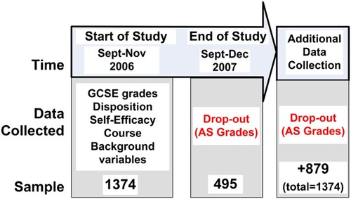
Of particular interest for this paper is the educational outcome ‘AS grade’ highlighted in the final data point of Figure 1. This variable was only requested from students at the final data point (because this is when it would have been available) and was the cause of much of the missing data, given the large attrition rates at this stage of the study. Fortunately, many of these missing data points for ‘AS grade’ were accessed at a later date by collecting data directly from the schools and the students via additional telephone surveys. With this approach we have been able to fill in the grades for 879 additional pupils.

This supplementary collection of much of the missing data from the study enabled an evaluation to be made of the success of data imputation. We compare the results of analyses conducted on the data which was initially available with the enhanced, supplementary data and evaluate the success of the imputation technique for replacing the missing data.

4. Analysis/results: modelling dropout from mathematics

We were particularly interested in modelling whether or not students dropped out of the mathematics courses they were enrolled on (as derived from the original outcome variable of ‘AS grade’). In the original study, this ‘drop-out’ variable was found to be related to the type of course they were on, their previous GCSE¹⁰ results in mathematics, their disposition to study mathematics at a higher level, and their self-efficacy rating (see Hutcheson, Pampaka, and Williams 2011 for a full description of the model selection procedure). The model reported for the full data was

Drop-out ∼ Course + Disposition + GCSE-grade + Maths Self Efficacy

where Drop-out and Course are binary categorical variables, GCSE-grade is an ordered categorical variable,¹¹ and Disposition and Maths Self Efficacy are continuous.

The analysis reported here is restricted to the data and the model used in Hutcheson, Pampaka and Williams (2011), which included the binary classifications of whether students had ‘dropped out' of the course that were retrieved after the initial study. In this paper, we model dropout using the initial data (n = 495) and compare the resulting model to a model where the missing dropout scores are imputed (n = 1374). An evaluation of the accuracy of the imputation is made by comparing the models with the one derived from the actual data that were recovered (n = 1374). The only difference between the imputed model and the one reported for the actual data is that the former includes 879 imputed values for dropout, whilst the latter includes 879 values for dropout that were retrieved after the initial study.

4.1. Modelling dropout using the initial data (n = 495)

Using the 495 data points available at the end of the initial study resulted in the model shown in Table 3.

Table 3. A logistic regression model of ‘dropout' using the 495 cases available at the end of the initial study.

Explanatory variables	Estimate	s.e.	z	p
(Intercept)	1.24	0.32	3.88	<.001
Course: UoM (ref:Trad)	−1.15	0.26	−4.45	<.001
Disposition	−0.09	0.05	−1.88	.06
GCSE-grade (ref: IntC)
Higher C	−0.44	0.57	−0.077	.44
Intermediate B	−0.46	0.32	−1.42	.16
Higher B	−0.67	0.34	−1.95	.05
A	−1.85	0.37	−5.07	<.001
A*	−4.9	1.06	−4.63	<.001
Maths Self Efficacy	−0.07	0.1	−0.68	.49

This model is, however, likely to provide a biased picture of dropout, as the missing data points are not likely to be ‘missing completely at random'. The non-random nature of the missing data is confirmed by analyses (i.e. a logistic regression model of ‘missingness’) which show that those with higher GCSE grades are more likely to have been included in the sample at the end of the initial study. The results of the logistic regression for ‘missingness’ (i.e. a binary variable indicating that a student provided information at the end of study (1) or not (0), modelled with respect to the following explanatory variables: Course, Disposition, GCSE-grade, and Maths Self Efficacy) are shown in Table 4 and the effects of the explanatory variables are illustrated via the effect plots in Figure 2 (Fox 1987; Fox and Hong 2009).

Figure 2. Effect plots of a logistic regression model of missingness on dropout variable. The graphs show the size of the effect of the explanatory variables on the response variable Y (i.e. the probability of providing information, thus not missing). The Y range is set to be the same for all graphs in order for the relative effects to be comparable.

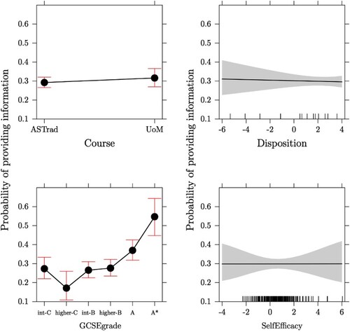
Table 4. A logistic regression model of missingness on dropout variable.

Explanatory variables	Estimate	s.e.	z	p
Intercept	−0.99	0.17	−5.87	<.001
Course UoM (ref:Trad)	0.11	0.14	0.81	.42
Disposition	−0.01	0.03	−0.27	.79
GCSE-grade (ref: IntC)
Higher C	−0.6	0.3	−1.99	.05
Intermediate B	−0.04	0.18	−0.22	.82
Higher B	0.01	0.19	0.08	.94
A	0.44	0.2	2.27	.02
A*	1.17	0.26	4.49	<.001
Maths Self Efficacy	0.00	0.05	0.01	.99

The logistic regression in Table 4 clearly shows the difference between GCSE grades for those students for whom information about dropout is available at the end of the initial study and those for whom it is not. The difference is particularly clear in the case of the students with A* grades, as these students are more than three times as likely (exp(1.17) = 3.22 times) to provide information about dropout than those with an intermediate-C grade (IntC).

Given these missingness patterns, the model in Table 3 is, therefore, likely to overestimate the effect of the high-achieving pupils.

4.2. Modelling dropout using imputed data

In order to address the likely bias in the sample of 495 cases, the 879 missing data points were imputed. We selected the Amelia II package (Honaker, King and Blackwell 2011) which imputes missing data using MI and includes a number of options and diagnostics using a simple graphical interface, and is implemented in the R statistical programme (R Core Team 2013). Amelia II assumes that the complete data are multivariate normal which is ‘often a crude approximation to the true distribution of the data’; however, there is ‘evidence that this model works as well as other, more complicated models even in the face of categorical or mixed data' (Honaker, King, and Blackwell 2013, 4). Amelia II also makes the usual assumption in MI that the data are missing at random (MAR), which means that the pattern of missingness only depends on the observed data and not the unobserved. The model we presented in Table 4 and Figure 2 shows that missingness depends on GCSE grades, which is an observed variable. Finally, the missing data points in the current analysis are binary, making Amelia an appropriate choice.

The missing values for dropout were imputed using a number of variables available in the full data set. In addition to using information about Course, Disposition, GCSE-grade, and Maths Self Efficacy to model the missing data, information about EMA (i.e. whether the student was holding Educational Maintenance Allowance), ethnicity, gender, Language (whether the student's first language was English), LPN (i.e. whether the student was from Low Participation Neighbourhood), uniFAM (whether the student was not first generation at HE), and HEFCE (an ordered categorical variable denoting socio-economic status) were also included.¹² Although relatively few imputations are often required (3–10, see Rubin 1987), it is recommended that more imputations are used when there are substantial amounts of missing data. For this analysis, we erred on the side of caution and used 100 imputed data sets.

Amelia imputed 100 separate data sets, each of which could have been used to model dropout. In order to get parameter estimates for the overall imputed model, models computed on the individual data sets were combined. The combined estimates and standard errors for the imputed model were then obtained using the Zelig library (Owen et al. 2013) from the R package. The overall statistics for the imputed models computed using Zelig are shown in Table 5, with the software instructions provided in Appendix.

Table 5. A logistic regression model of ‘dropout' using imputed data (n = 1374).

Explanatory variables	Estimate	s.e.	t-stat	p
Intercept	1.16	0.26	4.53	<.001
Course UoM (ref:Trad)	−0.87	0.22	−3.96	<.001
Disposition	−0.08	0.04	−1.89	.06
GCSE-grade (ref: IntC)
Higher C	−0.36	0.34	−1.05	.29
Intermediate B	−0.64	0.23	−2.73	.007
Higher B	−0.95	0.26	−3.66	.0003
A	−1.55	0.259	−5.32	<.001
A*	−2.74	0.46	−5.96	<.001
Maths Self Efficacy	−0.06	0.08	−0.71	.48

The conclusions for the model based on the imputed data are broadly the same as for the model with missing data (n = 495), with Course and GCSE-grade both showing significance. Disposition and Self Efficacy are non-significant in both models. The main difference between the models is found in the standard error estimates for the GCSE grades (the regression coefficients for the models are broadly similar across the two models) with the imputed data model allowing for a greater differentiation of ‘GCSE-grade’, with significant differences demonstrated between more categories compared to the initial model (the Higher B and Intermediate B groups are now significantly different to the reference category).

4.3. Modelling dropout using the retrieved data (n = 1374)

An evaluation of the success of the imputation can be obtained by comparing the results with that from a model computed on the actual data. A model of dropout using all available data (i.e. including the 879 data points retrieved after the initial study) results in the model shown in Table 6 (this is the same model reported in Hutcheson, Pampaka, and Williams 2011).

Table 6. A logistic regression model of ‘dropout' using the full/retrieved data (n = 1374).

Explanatory variables	Estimate	s.e.	z	p
(Intercept)	1.62	0.2	7.99	<.001
Course UoM (ref:Trad)	−1.29	0.16	−8.11	<.001
Disposition	−0.13	0.03	−4.56	<.001
GCSE-grade (ref: IntC)
Higher C	−0.26	0.30	−0.89	.38
Intermediate B	−0.88	0.2	−4.39	<.001
Higher B	−1.02	0.21	−4.86	<.001
A	−2.25	0.24	−9.56	<.001
A*	−3.83	0.5	−7.65	<.001
Maths Self Efficacy	−0.18	0.06	−3.20	<.01

4.4. Comparing all models

It is useful at this point to compare the results from all three models (Table 7).

Table 7. Parameter estimates for the three models.

Explanatory variables	Model with missing data (n = 495)	Model with imputed data	Model using full data (n = 1374)
	est, (s.e.), p	est, (s.e.), p	est, (s.e.), p
Course UoM (ref:Trad)	−1.15, (0.26), <.001	−0.87, (0.22), <.001	−1.29, (0.16), <.001
Disposition	−0.09, (0.05), .06	−0.08, (0.04), .06	−0.13, (0.03), <.001
GCSE-grade (ref: IntC)
Higher C	−0.44, (0.57), .44	−0.36, (0.34), .29	−0.26, (0.29), .38
Intermediate B	−0.46, (0.32), .16	−0.64, (0.23), .007	−0.88, (0.20), <.001
Higher B	−0.67, (0.34), .05	−0.95, (0.26), <.001	−1.02, (0.21), <.001
A	−1.85, (0.37), <.001	−1.55, (0.26), <.001	−2.25, (0.24), <.001
A*	−4.90, (1.06), <.001	−2.74, (0.46), <.001	−3.83, (0.50), <.001
Maths Self Efficacy	−0.07, (0.1), .49	−0.06, (0.08), .48	−0.18, (0.06), <.01

The estimates from all models provide similar pictures of the relationships in the data (all estimates are in the same direction). Even though the imputed model is not ‘equivalent’ to the model using the full data, the most noticeable finding is that the standard errors for the imputed model are lower than they are for the model with missing data and closer to the standard errors evident in the model on the actual data that were subsequently retrieved (particularly with respect to GCSE grades). In particular, compared to the model with missing data (n = 495), the imputed model allows a more accurate picture of the relationship between dropout and the GCSE-grade categories, showing the effect of the lower grades of GCSE on dropout more clearly.

Whilst this has not substantially affected the conclusions that were drawn from this study, the reduced bias may have been influential if the study had not in fact collected all this extra data, and we would expect it to be important in smaller studies where such effect sizes are declared insignificant. In any case, the imputed model provides a closer approximation to the full/retrieved data set than does the initial model on the 495 data points.

5. Discussion and conclusions

Our aim with this paper was to revisit and review the topic of dealing with non-response in the context of educational research, drawing from our recent work in widening participation in mathematics education. In addition, we wanted to assess the accuracy of MI using an example where models from imputed data could be compared with models derived from actual data.

First, we argued, as the literature in social statistics suggests, that ignoring missing data can have serious consequences in educational research contexts. Missing data are effectively ignored when using ‘complete case' analyses and the automated use of step-wise selection procedures often exacerbates this as cases can easily be excluded on the basis of data missing from variables not even part of a final model. Ignoring missing data causes problems when the data are not missing completely at random, as is likely for most missing data in educational research. We then demonstrated a procedure for how to deal with missing data with MI applied to our own (problematic) data set, which we could also verify given additional data acquired at a later stage. This procedure can be used by any (educational) researcher facing similar missing data problems and is summarized here for guidance (we also provide more technical details of these steps, apart from the former, as applied to our own analysis in Appendix):

1. identify missing data (with descriptive statistics);

2. investigate missing data patterns (e.g. by modelling missingness we find that students with lower grades are more likely to be missing);

3. define variables in the data set which may be related to missing values to be used for the imputation model (as resulted from modelling missingness);

4. impute missing data to give ‘m' complete data sets;

5. run the models of interest using the ‘m' imputed data sets;

6. combine the ‘m' models' parameters;

7. report the final model (as you would have done for any regression model).

In our own data set, the models did not in fact change much as a result of imputing missing data, but we were able to show that imputation improved the models and caused differences to the significance of the effects of some of the important variables. The results from our study demonstrated that the initial data sample which included a substantial amount of missing data was likely to be biased, as a regression model using this data set was quite different from the one based on a more complete data set that included information subsequently collected.

Imputing the missing data proved to be a useful exercise, as it ‘improved' the model, particularly with respect to the parameters for GCSE-grade, but it is important to note that it did not entirely recreate the structure of the full data set, as Disposition and Maths Self Efficacy remained non-significant. This, however, is not that surprising given these variables were insignificant in the original sample of 495, and it could also be due to the self-report nature of these variables in comparison to more robust GCSE grades. The failure to reconstruct the results from the full data set is not so much a failure of the MI technique, but a consequence of the initial model (where Disposition and Maths Self Efficacy were not significant). The information available to impute the missing dropout data points was not sufficient to accurately recreate the actual relationships between these variables. Incorporating additional information in the imputation process might have rectified this to some extent.¹³

The results of the MI are encouraging, particularly as the amount of missing data was relatively large (over 60% for dropout) and also missing on a ‘simple' binary variable. It is also worth noting that the model evaluated is one which shows a high degree of imprecision (Nagelkerke's pseudo-R² = 0.237 for the full data set). There is, therefore, likely to also be substantial imprecision in the imputed data. This empirical study demonstrates that even with this very difficult data set, MI still proved to be useful.

The imputation process was a useful exercise in understanding the data and the patterns of missingness. In this study, the model based on imputed data was broadly similar to the model based on the original data (n = 495). This finding does not diminish the usefulness of the analysis, as it reinforces the evidence that the missing data may not have heavily biased this model. In cases where there is more substantial bias, larger discrepancies between the imputed and non-imputed models may be expected. For the current data, even though the missing data were not particularly influential, the imputation was still advantageous.

The most important conclusion from this paper is that missing data can have adverse effects on analyses and imputation methods should be considered when this is an issue. This study shows the value of MI even when imputing large amounts of missing data points for a binary outcome variable. It is encouraging that tools now exist to enable MI to be applied relatively simply using easy-to-access software (see Hutcheson and Pampaka, 2012, for a review). Thus, MI techniques are now within the grasp of most educational researchers and should be used routinely in the analysis of educational data.

Acknowledgements

As authors of this paper we acknowledge the support of The University of Manchester. We are grateful for the valuable feedback of the anonymous reviewer(s).

Supplemental data

Supplemental data for this article can be accessed at http://research-training.net/missingdata/

Additional information

Funding

This work was supported by the Economic and Social Research Council (ESRC) through various grant awards: The Transmaths (www.transmaths.org) projects [RES-062-23-1213 and RES-139-25-0241] investigated the transition of students into post-compulsory mathematics education, and the most recent Teleprism (www.teleprism.com) study [RES-061-025-0538] explores the progression in Secondary education, whilst dealing with methodological challenges, including missing data.

Notes

1. List-wise deletion is one traditional statistical method for handling missing data, which entails an entire record being excluded from analysis if any single item/question value is missing. An alternative approach is pairwise deletion, when the case is excluded only from analyses involving variables that have missing values.

2. Selection methods here refer to the procedures followed for the selection of explanatory variables in regression modelling. In step-wise selection methods, the choice of predictive/explanatory variables is carried out by an automatic procedure. The most widely used step-wise methods are backward elimination (i.e. start with all possible variables and continue by excluding iteratively the less significant) and forward selection (i.e. starting with no explanatory variables and adding iteratively the most significant).

3. The same applies with popular packages such as SPSS where the only way to infer about the sample size used for each model is to check the degrees of freedom in the ANOVA table.

4. Some statistical packages automatically delete all cases list-wise (SPSS, for example), while others (e.g. the ‘step()' procedure implemented in R (R Development Core team 2013)) do not allow step-wise regression to be easily applied in the presence of missing data – when the sample size changes as a result of variables being added or removed, the procedure halts.

5. It has been shown by Rubin in 1987 that the relative efficiency of an estimate based on m imputations to one based on an infinite number of them approximates the inverse of (1+λ/m), with λ the rate of missing information. Based on this, it is also reported that there is no practical benefit in using more than 5–10 imputations (Schafer 1999; Schafer and Graham 2002).

6. ML estimation is a statistical method for estimating population parameters (i.e. mean and variance) from sample data that selects as estimates those parameter values maximizing the probability of obtaining the observed data (http://www.merriam-webster.com/dictionary/maximum%20likelihood).

7. From a statistical point of view $P(Y_{\mathrm{complete}};\theta )$ has two possible interpretations, which guide the choice of estimation methods for dealing with missing data:

• •when regarded as the repeated-sampling distribution for Y_complete, it describes the probability of obtaining any specific data set among all the possible data sets that could arise over hypothetical repetitions of the sampling procedure and data collection;

• •when considered as a likelihood function for theta (unknown parameter), the realized value of Y_complete is substituted into P and the resulting function for theta summarizes the data's evidence about parameters.

8. Bayesian statistical methods assign probabilities or distributions to events or parameters (e.g. a population mean) based on experience or best guesses (more formally defined as prior distributions) and then apply Bayes’ theorem to revise the probabilities and distributions after considering the data, thus resulting in what is formally defined as posterior distribution.

9. In England, it is compulsory to study mathematics up until the age of 16. Post-16 students can opt to take four advanced-subsidiary subjects (AS levels) of their choice, which are then typically refined to advanced-level (A-level or A2) subjects at the age of 17.

10. GCSE qualifications are usually taken at the end of compulsory education in a range of subjects. Students typically take about 8–10 of these in a range of subjects that must include English and mathematics.

11. GCSE-grade was treated as categorical variable in the model in the usual way: the lower grade was chosen as the reference category and the other categories were treated as dummy variables.

12. Although not part of the regression model

it is often useful to add more information to the imputation model than will be present when the analysis is run. Since imputation is predictive, any variables that would increase predictive power should be included in the model, even if including them would produce bias in estimating a causal effect or collinearity would preclude determining which variables had a relationship with the dependent variable. (Honaker, King and Blackwell 2013)

13. It is important to collect data that may aid the imputation process even if these data are not part of the final model.

Appendix

Technical details for performing MI

We present here more details of the steps followed during our implementation of the MI procedure summarized in the conclusion of the paper. The first descriptive analysis step as well as the final step of reporting the result is omitted. The steps presented here can be implemented with free open-access software that can be installed on any platform.

Step 2: Investigate missing data patterns.

Step 3: Identify variables related to the missing values.

The analysis that identified imbalances in the distribution of missing data was a logit regression model of missing values for the dropout variable. The R package was used for this analysis. The code below shows a logit model of missingness based on the explanatory variables:

glm(missingDATA ∼ Course + Disposition + GCSEgrade + SelfEfficacy, family=binomial(logit))

Step 4: Impute missing data to give ‘m' complete data sets.

The missing data are then imputed using the R library ‘Amelia' (version 1.7.2; Honaker, King, and Blackwell 2013). The code to achieve this is shown below, although imputations can also be obtained through a graphical interface, which some users may find simpler (see Hutcheson and Pampaka 2012):

imp.datasets <- amelia(Dataset, m=100,

noms=c("DROPout", "Course", "Gender", "Language",

"EMA", "Ethnicity", "LPN", "uniFAM"),

ords="GCSEgrade")

The command above instructs amelia to impute 100 data sets (m = 100) using nominal (noms) and ordinal (ords) variables and save these to the object ‘imp.datasets'. The ‘imp.datasets' object holds 100 data sets containing the imputed values, each of which can be viewed or analysed separately using the command:

imputed.datasets$imputations[[i]]

For example, the third imputed data set is saved as imputed.datasets$imputations[[3]].

Step 5: Run the models of interest using the ‘m' imputed data sets.

Step 6: Combine the model's parameters.

The logit regression model of dropout (our response variable of interest) can be applied to each of the imputed data sets, which results in 100 different models for the imputed data. These 100 models need to be combined to provide single parameter estimates across all the imputed data. An easy method for this is to use the R library ‘Zelig' (Owen et al. 2013). Zelig first computes models for each individual imputed data set and saves analyses to the object ‘Zelig.model.imp':

Zelig.model.imp <- zelig(DROPout ∼ Course + Disposition +

GCSEgrade + SelfEfficacy,

model = "logit",

data = imputed.datasets$imputations)

which can then be shown/printed out using the command:

summary(Zelig.model.imp, subset = 1:100)

References

- ACME. 2009. The Mathematics Education Landscape in 2009. A report of the Advisory Committee on Mathematics Education (ACME) for the DCSF/DIUS STEM high level strategy group meeting, June 12. Accessed March 1, 2010. http://www.acme-uk.org/downloaddoc.asp?id=139
- Allison, P. D. 2000. “Multiple Imputation for Missing Data: A Cautionary Tale.” Sociological Methods and Research 28 (3): 301–309. doi: 10.1177/0049124100028003003
- Durrant, G. B. 2009. “Imputation Methods for Handling Item Non-response in Practice: Methodological Issues and Recent Debates.” International Journal of Social Research Methodology 12 (4): 293–304. doi: 10.1080/13645570802394003
- Fox, J. 1987. “Effect Displays for Generalized Linear Models.” Sociological Methodology 17: 347–361. doi: 10.2307/271037
- Fox, J., and J. Hong. 2009. “The Effects Package. Effect Displays for Linear, Generalized Linear, Multinomial-Logit, and Proportional-Odds Logit Models.” Journal of Statistical Software 32 (1): 1–24. doi: 10.18637/jss.v032.i01
- Gottardo, R. 2004. “EMV: Estimation of Missing Values for a Data Matrix.” Accessed January 15, 2014. http://ftp.auckland.ac.nz/software/CRAN/doc/packages/EMV.pdf
- Harrell, F. E. 2008. “Hmisc: Harrell Miscellaneous.” Accessed January 15, 2014. http://cran.r-project.org/web/packages/Hmisc/index.html
- Hastie, T., R. Tibshirani, B. Narasimhan, and G. Chu. 2014. “Impute: Imputation for Microarray Data.” R Package Version 1.32.0. Accessed January 15, 2014. http://www.bioconductor.org/packages/release/bioc/manuals/impute/man/impute.pdf
- Honaker, J., and G. King. 2010. “What to Do about Missing Values in Time-Series Cross-section Data.” American Journal of Political Science 54 (2): 561–581. doi: 10.1111/j.1540-5907.2010.00447.x
- Honaker, J., G. King, and M. Blackwell. 2011. “Amelia II: A Programme for Missing Data.” Journal of Statistical Software 45 (7): 1–47. doi: 10.18637/jss.v045.i07
- Honaker, J., G. King, and M. Blackwell. 2013. “Amelia II: A Program for Missing Data.” Accessed January 15, 2014. http://cran.r-project.org/web/packages/Amelia/vignettes/amelia.pdf
- Horton, N. J., and K. P. Kleinman. 2007. “Much Ado about Nothing: A Comparison of Missing Data Methods and Software to Fit Incomplete Data Regression Models.” The American Statistician 61 (1): 79–90. doi: 10.1198/000313007X172556
- Hutcheson, G. D., and M. Pampaka. 2012. “Missing Data: Data Replacement and Imputation (Tutorial).” Journal of Modelling in Management 7 (2): 221–233. doi: 10.1108/jm2.2012.29707baa.002
- Hutcheson, G. D., M. Pampaka, and J. Williams. 2011. “Enrolment, Achievement and Retention on ‘Traditional’ and ‘Use of Mathematics’ Pre-university Courses.” Research in Mathematics Education 13 (2): 147–168. doi: 10.1080/14794802.2011.585827
- Ibrahim, J. G., M.-H. Chen, S. R. Lipsitz, and A.H. Herring. 2005. “Missing-Data Methods for Generalized Linear Models.” Journal of the American Statistical Association 100 (469): 332–346. doi: 10.1198/016214504000001844
- Kim, J. K., and W. Fuller. 2004. “Fractional Hot Deck Imputation.” Biometrika 91 (3): 559–578. doi: 10.1093/biomet/91.3.559
- King, G., J. Honaker, A. Joseph, and K. Scheve. 2001. “Analyzing Incomplete Political Science Data: An Alternative Algorithm for Multiple Imputation.” American Political Science Review 95 (1): 49–69.
- Lee, E.-K., D. Yoon, and T. Park. 2009. “ArrayImpute: Missing Imputation for Microarray Data.” Accessed January 15, 2014. http://cran.uvigo.es/web/packages/arrayImpute/arrayImpute.pdf
- Little, R. J. A. 1988. “Missing-Data Adjustments in Large Surveys.” Journal of Business & Economic Statistics 6 (3): 287–296.
- Little, R. J. A., and D. B. Rubin. 1987. Statistical Analysis with Missing Data. New York: John Wiley & Sons.
- Little, R. J. A., and D. B. Rubin. 1989. “The Analysis of Social Science Data with Missing Values.” Sociological Methods Research 18 (2–3): 292–326. doi: 10.1177/0049124189018002004
- Nielsen, S. R. F. 2003. “Proper and Improper Multiple Imputation.” International Statistical Review/Revue Internationale de Statistique 71 (3): 593–607.
- Owen, M., O. Lau, K. Imai, and G. King. 2013. “Zelig v4.0-10 Core Model Reference Manual.” Accessed December 5, 2013. http://cran.r-project.org/web/packages/Zelig/
- Pampaka, M., I. Kleanthous, G. D. Hutcheson, and G. Wake. 2011. “Measuring Mathematics Self-efficacy as a Learning Outcome.” Research in Mathematics Education 13 (2): 169–190. doi: 10.1080/14794802.2011.585828
- Pampaka, M., J. S. Williams, G. Hutcheson, L. Black, P. Davis, P. Hernandez-Martines, and G. Wake. 2013. “Measuring Alternative Learning Outcomes: Dispositions to Study in Higher Education.” Journal of Applied Measurement 14 (2): 197–218.
- Pampaka, M., J. S. Williams, G. Hutcheson, G. Wake, L. Black, P. Davis, and P. Hernandez-Martinez. 2012. “The Association Between Mathematics Pedagogy and Learners’ Dispositions for University Study.” British Educational Research Journal 38 (3): 473–496. doi: 10.1080/01411926.2011.555518
- Plewis, I. 2007. “Non-response in a Birth Cohort Study: The Case of the Millennium Cohort Study.” International Journal for Social Research Methodology 10 (5): 325–334. doi: 10.1080/13645570701676955
- R Core Team. 2013. R: A Language and Environment for Statistical Computing. Vienna: R Foundation for Statistical Computing (ISBN 3-900051-07-0). http://www.R-project.org
- Reiter, J. P., and T. E. Raghunathan. 2007. “The Multiple Adaptations of Multiple Imputation.” Journal of the American Statistical Association 102 (480): 1462–1471. doi: 10.1198/016214507000000932
- Roberts, G. 2002. SET for Success. The Supply of People with Science, Technology, Engineering and Mathematics Skills. London: HM Stationery Office.
- Rubin, D. B. 1987. Multiple Imputation for Nonresponse in Surveys. New York: John Wiley.
- Rubin, D. B. 1996. “Multiple Imputation after 18+ Years.” Journal of the American Statistical Association 91 (434): 473–489. doi: 10.1080/01621459.1996.10476908
- Sainsbury, L. 2007. The Race to the Top: A Review of Government's Science and Innovation Policies. London: HM Stationery office.
- Schafer, J. L. 1997. Analysis of Incomplete Multivariate Data. London: Chapman & Hall.
- Schafer, J. L. 1999. “Multiple Imputation: A Primer.” Statistical Methods in Medical Research 8 (1): 3–15. doi: 10.1191/096228099671525676
- Schafer, J. L., and J. W. Graham. 2002. “Missing Data: Our View of the State of the Art.” Psychological Methods 7 (2): 147–177. doi: 10.1037/1082-989X.7.2.147
- Smith, A. 2004. Making Mathematics Count – the Report of Professor Adrian Smith's Inquiry into Post-14. Mathematics Education. London: DfES.
- Squire, P. 1988. “Why the 1936 Literary Digest Poll Failed.” Public Opinion Quarterly 52 (1): 125–133. doi: 10.1086/269085
- Su, Y.-S., A. Gelman, J. Hill, and M. Yajima. 2011. “Multiple Imputation with Diagnostics (mi) in R: Opening Windows into the Black Box.” Journal of Statistical Software 45 (2): 1–31. Accessed January 15, 2014. http://www.jstatsoft.org/v45/i02/ doi: 10.18637/jss.v045.i02
- Van Buuren, S., and K. Groothuis-Oudshoorn. 2011. “Mice: Multivariate Imputation by Chained Equations in R.” Journal of Statistical Software 45 (3): 1–67. Accessed December 5, 2013. http://www.jstatsoft.org/v45/i03/
- Wainer, H. 2010. “14 Conversations about Three Things.” Journal of Educational and Behavioral Statistics 35 (1): 5–25. doi: 10.3102/1076998609355124
- Wayman, J. C. 2003. “Multiple Imputation for Missing Data: What Is It and How Can I Use It?” Annual Meeting of the American Educational Research Association, Chicago, IL.
- Williams, J. S., L. Black, P. Davis, P. Hernandez-Martinez, G. Hutcheson, S. Nicholson, M. Pampaka, and G. Wake. 2008. TLRP Research Briefing No 38: Keeping Open the Door to Mathematically Demanding Programmes in Further and Higher Education. School of Education, University of Manchester.
- Zhang, P. 2003. “Multiple Imputation: Theory and Method.” International Statistical Review 71 (3): 581–592. doi: 10.1111/j.1751-5823.2003.tb00213.x