Optimal stopping problems for maxima and minima in models with asymmetric information

Abstract

We derive closed-form solutions to optimal stopping problems related to the pricing of perpetual American withdrawable standard and lookback put and call options in an extension of the Black-Merton-Scholes model with asymmetric information. It is assumed that the contracts are withdrawn by their writers at the last hitting times for the underlying risky asset price of its running maximum or minimum over the infinite time interval which are not stopping times with respect to the observable filtration. We show that the optimal exercise times are the first times at which the asset price process reaches some lower or upper stochastic boundaries depending on the current values of its running maximum or minimum. The proof is based on the reduction of the original necessarily two-dimensional optimal stopping problems to the associated free-boundary problems and their solutions by means of the smooth-fit and normal-reflection conditions. We prove that the optimal exercise boundaries are the maximal and minimal solutions of some first-order nonlinear ordinary differential equations.

Keywords:

• Optimal stopping problem
• Brownian motion
• last hitting time
• asymmetric information
• first passage time
• running maximum and minimum processes
• stochastic boundary
• free-boundary problem
• instantaneous stopping and smooth fit
• normal reflection
• a change-of-variable formula with local time on surfaces
• perpetual American standard and lookback options

1. Introduction

Let us consider a probability space $(\mathrm{\Omega },\mathcal{F},P)$ with a standard Brownian motion $B=(B_t{)}_{t\ge 0}$ and define the process $X=(X_t{)}_{t\ge 0}$ by: (1) $X_t=x\exp ((r-\delta -{\sigma }^2/2)t+\sigma B_t)$(1) which solves the stochastic differential equation: (2) $\mathrm{d}{X}_t=(r-\delta )X_t\mathrm{d}t+\sigma X_t\mathrm{d}{B}_t(X_0=x)$(2) where x>0 is fixed, and r>0, $\delta >0$, and $\sigma >0$ are some given constants. Assume that the process X describes the price of a risky asset in a financial market, where r is the riskless interest rate, δ is the dividend rate paid to the asset holders, and σ is the volatility rate.

We aim to present closed-form solutions to the discounted optimal stopping problems with the values: (3) ${\overline{V}}_i=\underset{\tau }{sup}E[{\mathrm{e}}^{-r(\tau \wedge \theta )}{G}_i(X_{\tau \wedge \theta },S_{\tau \wedge \theta })]\mathrm{and}{\overline{U}}_i=\underset{\zeta }{sup}E[{\mathrm{e}}^{-r(\zeta \wedge \eta )}{F}_i(X_{\zeta \wedge \eta },Q_{\zeta \wedge \eta })]$(3) with $G_1(x,s)=L_1-x$, $G_2(x,s)=s-L_{2}x$, $G_3(x,s)=s-L_3$ and $F_1(x,q)=x-K_1$, $F_2(x,q)=K_{2}x-q$, $F_3(x,q)=K_3-q$, for some deterministic constants $L_i,K_i>0$, for i = 1, 2, 3. Suppose that the suprema in (3(3) ${\overline{V}}_i=\underset{\tau }{sup}E[{\mathrm{e}}^{-r(\tau \wedge \theta )}{G}_i(X_{\tau \wedge \theta },S_{\tau \wedge \theta })]\mathrm{and}{\overline{U}}_i=\underset{\zeta }{sup}E[{\mathrm{e}}^{-r(\zeta \wedge \eta )}{F}_i(X_{\zeta \wedge \eta },Q_{\zeta \wedge \eta })]$(3) ) are taken over all stopping times τ and ζ with respect to the filtration $({\mathcal{F}}_t{)}_{t\ge 0}$. The linear functions $G_i(x,s)$ and $F_i(x,q)$, for i = 1, 2, 3, represent the payoffs of standard and lookback options with floating and fixed strikes, respectively, which are widely used in financial practice. Here, the random times θ and η given by: (4) $\theta =sup\{t\ge 0|X_t=S_t\}\mathrm{and}\eta =sup\{t\ge 0|X_t=Q_t\}$(4) are not stopping times with respect to the natural filtration $({\mathcal{F}}_t{)}_{t\ge 0}$ of the process X, but they are honest times in the sense of Nikeghbali and Yor [34]. The processes $S=(S_t{)}_{t\ge 0}$ and $Q=(Q_t{)}_{t\ge 0}$ are the running maximum and minimum of X defined by: (5) $S_t=s\vee \left(\underset{0\le u\le t}{max}{X}_u\right)\mathrm{and}{Q}_t=q\wedge \left(\underset{0\le u\le t}{min}{X}_u\right)$(5) for some arbitrary $0<q\le x\le s$.

Although the random times θ and η are not stopping times of X, we can still reduce the problems of (3(3) ${\overline{V}}_i=\underset{\tau }{sup}E[{\mathrm{e}}^{-r(\tau \wedge \theta )}{G}_i(X_{\tau \wedge \theta },S_{\tau \wedge \theta })]\mathrm{and}{\overline{U}}_i=\underset{\zeta }{sup}E[{\mathrm{e}}^{-r(\zeta \wedge \eta )}{F}_i(X_{\zeta \wedge \eta },Q_{\zeta \wedge \eta })]$(3) ) to the associated optimal stopping problems for the two-dimensional (time-homogeneous strong) continuous Markov processes $(X,S)$ and $(X,Q)$. For this purpose, we observe that the expected rewards from (3(3) ${\overline{V}}_i=\underset{\tau }{sup}E[{\mathrm{e}}^{-r(\tau \wedge \theta )}{G}_i(X_{\tau \wedge \theta },S_{\tau \wedge \theta })]\mathrm{and}{\overline{U}}_i=\underset{\zeta }{sup}E[{\mathrm{e}}^{-r(\zeta \wedge \eta )}{F}_i(X_{\zeta \wedge \eta },Q_{\zeta \wedge \eta })]$(3) ) admit the representations: (6) $E[{\mathrm{e}}^{-r(\tau \wedge \theta )}{G}_i(X_{\tau \wedge \theta },S_{\tau \wedge \theta })]=E[{\mathrm{e}}^{-r\tau }{G}_i(X_{\tau },S_{\tau })I(\tau <\theta )+{\mathrm{e}}^{-r\theta }{G}_i(S_{\theta },S_{\theta })I(\theta \le \tau )]$(6) and (7) $E[{\mathrm{e}}^{-r(\zeta \wedge \eta )}{F}_i(X_{\zeta \wedge \eta },Q_{\zeta \wedge \eta })]=E[{\mathrm{e}}^{-r\zeta }{F}_i(X_{\zeta },Q_{\zeta })I(\zeta <\eta )+{\mathrm{e}}^{-r\eta }{F}_i(Q_{\eta },Q_{\eta })I(\eta \le \zeta )]$(7) for i = 1, 2, 3. Observe that the expressions in (6(6) $E[{\mathrm{e}}^{-r(\tau \wedge \theta )}{G}_i(X_{\tau \wedge \theta },S_{\tau \wedge \theta })]=E[{\mathrm{e}}^{-r\tau }{G}_i(X_{\tau },S_{\tau })I(\tau <\theta )+{\mathrm{e}}^{-r\theta }{G}_i(S_{\theta },S_{\theta })I(\theta \le \tau )]$(6) ) and (7(7) $E[{\mathrm{e}}^{-r(\zeta \wedge \eta )}{F}_i(X_{\zeta \wedge \eta },Q_{\zeta \wedge \eta })]=E[{\mathrm{e}}^{-r\zeta }{F}_i(X_{\zeta },Q_{\zeta })I(\zeta <\eta )+{\mathrm{e}}^{-r\eta }{F}_i(Q_{\eta },Q_{\eta })I(\eta \le \zeta )]$(7) ) allow to describe the original contracts as standard game (or Israeli) contingent claims introduced by Kifer [27]. Such contracts enable their issuers to exercise their right to withdraw the contracts prematurely, by paying some penalties agreed in advance. Further developments of the Israeli options and the associated zero-sum optimal stopping (Dynkin) games were provided by Kyprianou [29], Kühn and Kyprianou [28], Kallsen and Kühn [26], Baurdoux and Kyprianou [3–5], Ekström and Villeneuve [12], Ekström and Peskir [11], Baurdoux, Kyprianou and Pardo [6], Egami, Leung, and Yamazaki [10], and Leung and Yamazaki [31] among others. In contrast to the concept of game contingent claims mentioned above, in the present paper, we study the withdrawable American standard and lookback options in which the writers can terminate the contracts prematurely, by taking advantage of insider information which is not available to the holders. More precisely, we suppose that the option writers know the last hitting times for the underlying risky asset price process of its running maximum or minimum θ or η over the infinite time interval, respectively. For instance, such situations can occur when the writers issue options on the underlying risky assets which may represent the shares of either their own firms or other companies to the decisions of the board of which they have access and potentially influence them. In this view, the values ${\overline{V}}_i$ and ${\overline{U}}_i$, for i = 1, 2, 3, in (3(3) ${\overline{V}}_i=\underset{\tau }{sup}E[{\mathrm{e}}^{-r(\tau \wedge \theta )}{G}_i(X_{\tau \wedge \theta },S_{\tau \wedge \theta })]\mathrm{and}{\overline{U}}_i=\underset{\zeta }{sup}E[{\mathrm{e}}^{-r(\zeta \wedge \eta )}{F}_i(X_{\zeta \wedge \eta },Q_{\zeta \wedge \eta })]$(3) ) can be interpreted as the rational (or no-arbitrage) prices of the perpetual American withdrawable options in the appropriate extension of the Black-Merton-Scholes model (see, e.g. [45, Chapter VII, Section 3g]). Some extensive overviews of the perpetual American options in diffusion models of financial markets and other related results in the area are provided in Shiryaev [45, Chapter VIII; Section 2a], Peskir and Shiryaev [41, Chapter VII; Section 25], and Detemple [8] among others.

We further study the problems of (3(3) ${\overline{V}}_i=\underset{\tau }{sup}E[{\mathrm{e}}^{-r(\tau \wedge \theta )}{G}_i(X_{\tau \wedge \theta },S_{\tau \wedge \theta })]\mathrm{and}{\overline{U}}_i=\underset{\zeta }{sup}E[{\mathrm{e}}^{-r(\zeta \wedge \eta )}{F}_i(X_{\zeta \wedge \eta },Q_{\zeta \wedge \eta })]$(3) ) as the associated optimal stopping problems of (25(25) $V_i^{\ast }(x,s)=\underset{\tau }{sup}{E}_{x,s}[{\int }_0^{\tau }{\mathrm{e}}^{-ru}{H}_{i,1}(X_u,S_u)\mathrm{d}u+{\int }_0^{\tau }{\mathrm{e}}^{-ru}{\mathrm{\partial }}_s{G}_i(S_u,S_u)\mathrm{d}{S}_u]$(25) ) and (26(26) $U_i^{\ast }(x,q)=\underset{\zeta }{sup}{E}_{x,q}[{\int }_0^{\zeta }{\mathrm{e}}^{-ru}{H}_{i,2}(X_u,Q_u)\mathrm{d}u+{\int }_0^{\zeta }{\mathrm{e}}^{-ru}{\mathrm{\partial }}_q{F}_i(Q_u,Q_u)\mathrm{d}{Q}_u]$(26) ) for the two-dimensional continuous Markov processes having the underlying risky asset price X and its running maximum S or minimum Q as their state space components. The resulting problems turn out to be necessarily two-dimensional in the sense that they cannot be reduced to optimal stopping problems for one-dimensional Markov processes. Note that the integrals in the reward functionals of the optimal stopping problems in (25(25) $V_i^{\ast }(x,s)=\underset{\tau }{sup}{E}_{x,s}[{\int }_0^{\tau }{\mathrm{e}}^{-ru}{H}_{i,1}(X_u,S_u)\mathrm{d}u+{\int }_0^{\tau }{\mathrm{e}}^{-ru}{\mathrm{\partial }}_s{G}_i(S_u,S_u)\mathrm{d}{S}_u]$(25) ) and (26(26) $U_i^{\ast }(x,q)=\underset{\zeta }{sup}{E}_{x,q}[{\int }_0^{\zeta }{\mathrm{e}}^{-ru}{H}_{i,2}(X_u,Q_u)\mathrm{d}u+{\int }_0^{\zeta }{\mathrm{e}}^{-ru}{\mathrm{\partial }}_q{F}_i(Q_u,Q_u)\mathrm{d}{Q}_u]$(26) ) contain complicated integrands depending on the asset price as well as its running maximum and minimum processes. This feature initiates further developments of techniques to determine the structure of the associated continuation and stopping regions as well as appropriate modifications of the normal-reflection conditions in the equivalent free-boundary problems. Moreover, we show that the appearance of the withdrawal opportunities for the writers of the contracts at the times θ and η may essentially change the behaviour of the optimal exercise boundaries for the holders of the options. The other problems of perpetual American cancellable or defaultable standard and lookback options in models with last passage times of constant and random levels for the underlying asset prices and zero or linear recoveries were recently considered in Gapeev, Li and Wu [21] and Gapeev and Li [16], respectively.

Discounted optimal stopping problems for the running maxima and minima of the initial continuous (diffusion-type) processes were initiated by Shepp and Shiryaev [44] and further developed by Pedersen [36], Guo and Shepp [24], Gapeev [14], Guo and Zervos [25], Peskir [39,40], Glover, Hulley, and Peskir [22], Gapeev and Rodosthenous [17–19], Rodosthenous and Zervos [43], Gapeev, Kort, and Lavrutich [20], and Gapeev and Al Motairi [15] among others. It was shown, by means of the maximality principle for solutions of optimal stopping stopping problems established by Peskir [37], which is equivalent to the superharmonic characterization of the value functions, that the optimal stopping boundaries are given by the appropriate extremal solutions of certain (systems of) first-order nonlinear ordinary differential equations. More complicated optimal stopping problems in models with spectrally negative Lévy processes and their running maxima were studied by Asmussen, Avram, and Pistorius [1], Avram, Kyprianou, and Pistorius [2], Ott [35], Kyprianou and Ott [30], and Li, Vu and Zhou [32] among others.

The rest of the paper is organized as follows. In Section 2, we embed the original problems of (3(3) ${\overline{V}}_i=\underset{\tau }{sup}E[{\mathrm{e}}^{-r(\tau \wedge \theta )}{G}_i(X_{\tau \wedge \theta },S_{\tau \wedge \theta })]\mathrm{and}{\overline{U}}_i=\underset{\zeta }{sup}E[{\mathrm{e}}^{-r(\zeta \wedge \eta )}{F}_i(X_{\zeta \wedge \eta },Q_{\zeta \wedge \eta })]$(3) ) into the optimal stopping problems of (25(25) $V_i^{\ast }(x,s)=\underset{\tau }{sup}{E}_{x,s}[{\int }_0^{\tau }{\mathrm{e}}^{-ru}{H}_{i,1}(X_u,S_u)\mathrm{d}u+{\int }_0^{\tau }{\mathrm{e}}^{-ru}{\mathrm{\partial }}_s{G}_i(S_u,S_u)\mathrm{d}{S}_u]$(25) ) and (26(26) $U_i^{\ast }(x,q)=\underset{\zeta }{sup}{E}_{x,q}[{\int }_0^{\zeta }{\mathrm{e}}^{-ru}{H}_{i,2}(X_u,Q_u)\mathrm{d}u+{\int }_0^{\zeta }{\mathrm{e}}^{-ru}{\mathrm{\partial }}_q{F}_i(Q_u,Q_u)\mathrm{d}{Q}_u]$(26) ) for the two-dimensional continuous Markov processes $(X,S)$ and $(X,Q)$ defined in (1(1) $X_t=x\exp ((r-\delta -{\sigma }^2/2)t+\sigma B_t)$(1) ) and (5(5) $S_t=s\vee \left(\underset{0\le u\le t}{max}{X}_u\right)\mathrm{and}{Q}_t=q\wedge \left(\underset{0\le u\le t}{min}{X}_u\right)$(5) ). It is shown that the optimal stopping times ${\tau }_i^{\ast }$ and ${\zeta }_i^{\ast }$ are the first times at which the process X reaches some lower or upper boundaries $a_i^{\ast }(S)$ or $b_i^{\ast }(Q)$ depending on the current values of the processes S or Q, for i = 1, 2, 3, respectively. In Section 3, we derive closed-form expressions for the associated value functions $V_i^{\ast }(x,s)$ and $U_i^{\ast }(x,q)$ as solutions to the equivalent free-boundary problems and apply the modified normal-reflection conditions at the edges of the two-dimensional state spaces for $(X,S)$ or $(X,Q)$ to characterize the optimal stopping boundaries $a_i^{\ast }(S)$ and $b_i^{\ast }(Q)$, for i = 1, 2, 3, as the maximal or minimal solutions to the resulting first-order nonlinear ordinary differential equations. In Section 4, by using the change-of-variable formula with local time on surfaces from Peskir [38], we verify that the solutions of the free-boundary problems provide the solutions of the original optimal stopping problems. The main results of the paper are stated in Theorems 2.1 and 4.1.

2. Preliminaries

In this section, we introduce the setting and notation of the two-dimensional optimal stopping problems which are related to the pricing of perpetual American withdrawable standard and lookback put and call options and formulate the equivalent free-boundary problems.

2.1. The optimal stopping problems

In order to compute the expectations in (6(6) $E[{\mathrm{e}}^{-r(\tau \wedge \theta )}{G}_i(X_{\tau \wedge \theta },S_{\tau \wedge \theta })]=E[{\mathrm{e}}^{-r\tau }{G}_i(X_{\tau },S_{\tau })I(\tau <\theta )+{\mathrm{e}}^{-r\theta }{G}_i(S_{\theta },S_{\theta })I(\theta \le \tau )]$(6) ) and (7(7) $E[{\mathrm{e}}^{-r(\zeta \wedge \eta )}{F}_i(X_{\zeta \wedge \eta },Q_{\zeta \wedge \eta })]=E[{\mathrm{e}}^{-r\zeta }{F}_i(X_{\zeta },Q_{\zeta })I(\zeta <\eta )+{\mathrm{e}}^{-r\eta }{F}_i(Q_{\eta },Q_{\eta })I(\eta \le \zeta )]$(7) ), let us now introduce the conditional survival processes $Z=(Z_t{)}_{t\ge 0}$ and $Y=(Y_t{)}_{t\ge 0}$ defined by $Z_t=P(\theta >t|{\mathcal{F}}_t)$ and $Y_t=P(\eta >t|{\mathcal{F}}_t)$, for all $t\ge 0$, respectively. Note that the processes Z and Y are called the Azéma supermartingales of the random times θ and η (see, e.g. [33, Section 1.2.1]). By using the fact that the global maximum of a Brownian motion with the drift coefficient $(r-\delta )/{\sigma }^2-1/2<0$ has an exponential distribution with the mean $1/(2(\delta -r)/{\sigma }^2+1)$, while the negative of the global minimum of a Brownian motion with the drift coefficient $(r-\delta )/{\sigma }^2-1/2>0$ has an exponential distribution with the mean $1/(2(r-\delta )/{\sigma }^2-1)$ (see, e.g. [42, Chapter II, Exercise 3.12]), we have: (8) $Z_t=\{\begin{array}{ll}(S_t/X_t{)}^{\alpha },& \mathrm{if}\alpha <0\\ 1,& \mathrm{if}\alpha \ge 0\end{array}\mathrm{and}{Y}_t=\{\begin{array}{ll}(Q_t/X_t{)}^{\alpha },& \mathrm{if}\alpha >0\\ 1,& \mathrm{if}\alpha \le 0\end{array}$(8) for all $t\ge 0$, under s = x and q = x, where we set $\alpha =2(r-\delta )/{\sigma }^2-1$, respectively. The representations in (8(8) $Z_t=\{\begin{array}{ll}(S_t/X_t{)}^{\alpha },& \mathrm{if}\alpha <0\\ 1,& \mathrm{if}\alpha \ge 0\end{array}\mathrm{and}{Y}_t=\{\begin{array}{ll}(Q_t/X_t{)}^{\alpha },& \mathrm{if}\alpha >0\\ 1,& \mathrm{if}\alpha \le 0\end{array}$(8) ) can also be obtained from applying Doob's maximal equality (see [34, Lemma 2.1 and Proposition 2.2]) to the process $X^{-\alpha }=(X_t^{-\alpha }{)}_{t\ge 0}$, which is a strictly positive continuous local martingale converging to zero at infinity. Then, it follows from a direct application of the tower property for conditional expectations that the first terms in the right-hand sides of the expressions in (6(6) $E[{\mathrm{e}}^{-r(\tau \wedge \theta )}{G}_i(X_{\tau \wedge \theta },S_{\tau \wedge \theta })]=E[{\mathrm{e}}^{-r\tau }{G}_i(X_{\tau },S_{\tau })I(\tau <\theta )+{\mathrm{e}}^{-r\theta }{G}_i(S_{\theta },S_{\theta })I(\theta \le \tau )]$(6) ) and (7(7) $E[{\mathrm{e}}^{-r(\zeta \wedge \eta )}{F}_i(X_{\zeta \wedge \eta },Q_{\zeta \wedge \eta })]=E[{\mathrm{e}}^{-r\zeta }{F}_i(X_{\zeta },Q_{\zeta })I(\zeta <\eta )+{\mathrm{e}}^{-r\eta }{F}_i(Q_{\eta },Q_{\eta })I(\eta \le \zeta )]$(7) ) have the form: (9) $E[{\mathrm{e}}^{-r\tau }{G}_i(X_{\tau },S_{\tau })I(\tau <\theta )]=E[{\mathrm{e}}^{-r\tau }{G}_i(X_{\tau },S_{\tau })(S_{\tau }/X_{\tau }{)}^{\alpha }]$(9) when $\alpha <0$, under s = x, and (10) $E[{\mathrm{e}}^{-r\zeta }{F}_i(X_{\zeta },Q_{\zeta })I(\zeta <\eta )]=E[{\mathrm{e}}^{-r\zeta }{F}_i(X_{\zeta },Q_{\zeta })(Q_{\zeta }/X_{\zeta }{)}^{\alpha }]$(10) when $\alpha >0$, under q = x, for any stopping times τ and ζ of the process X, respectively. Moreover, it follows from standard applications of Itô's formula (see, e.g. [42, Chapter IV, Theorem 3.3]) and the properties that the processes S and Q may change their values only when $X_t=S_t$ and $X_t=Q_t$, for $t\ge 0$, respectively, that the Azéma supermartingales Z and Y from (8(8) $Z_t=\{\begin{array}{ll}(S_t/X_t{)}^{\alpha },& \mathrm{if}\alpha <0\\ 1,& \mathrm{if}\alpha \ge 0\end{array}\mathrm{and}{Y}_t=\{\begin{array}{ll}(Q_t/X_t{)}^{\alpha },& \mathrm{if}\alpha >0\\ 1,& \mathrm{if}\alpha \le 0\end{array}$(8) ) admit the stochastic differentials: (11) $\mathrm{d}{Z}_t=-\alpha {\left(\frac{S_t}{X_t}\right)}^{\alpha }\sigma \mathrm{d}{B}_t+\alpha I(X_t=S_t){\left(\frac{S_t}{X_t}\right)}^{\alpha }\frac{\mathrm{d}{S}_t}{S_t}=-\alpha {\left(\frac{S_t}{X_t}\right)}^{\alpha }\sigma \mathrm{d}{B}_t+\alpha \frac{\mathrm{d}{S}_t}{S_t}$(11) when $\alpha <0$, and (12) $\mathrm{d}{Y}_t=-\alpha {\left(\frac{Q_t}{X_t}\right)}^{\alpha }\sigma \mathrm{d}{B}_t+\alpha I(X_t=Q_t){\left(\frac{Q_t}{X_t}\right)}^{\alpha }\frac{\mathrm{d}{Q}_t}{Q_t}=-\alpha {\left(\frac{Q_t}{X_t}\right)}^{\alpha }\sigma \mathrm{d}{B}_t+\alpha \frac{\mathrm{d}{Q}_t}{Q_t}$(12) when $\alpha >0$, respectively. Hence, it follows from Doob-Meyer decompositions for the processes Z and Y in (11(11) $\mathrm{d}{Z}_t=-\alpha {\left(\frac{S_t}{X_t}\right)}^{\alpha }\sigma \mathrm{d}{B}_t+\alpha I(X_t=S_t){\left(\frac{S_t}{X_t}\right)}^{\alpha }\frac{\mathrm{d}{S}_t}{S_t}=-\alpha {\left(\frac{S_t}{X_t}\right)}^{\alpha }\sigma \mathrm{d}{B}_t+\alpha \frac{\mathrm{d}{S}_t}{S_t}$(11) ) and (12(12) $\mathrm{d}{Y}_t=-\alpha {\left(\frac{Q_t}{X_t}\right)}^{\alpha }\sigma \mathrm{d}{B}_t+\alpha I(X_t=Q_t){\left(\frac{Q_t}{X_t}\right)}^{\alpha }\frac{\mathrm{d}{Q}_t}{Q_t}=-\alpha {\left(\frac{Q_t}{X_t}\right)}^{\alpha }\sigma \mathrm{d}{B}_t+\alpha \frac{\mathrm{d}{Q}_t}{Q_t}$(12) ) and applications of the dual predictable projection property (see, e.g. [34, Corollary 2.4]) that the second terms in the right-hand sides of the expressions in (6(6) $E[{\mathrm{e}}^{-r(\tau \wedge \theta )}{G}_i(X_{\tau \wedge \theta },S_{\tau \wedge \theta })]=E[{\mathrm{e}}^{-r\tau }{G}_i(X_{\tau },S_{\tau })I(\tau <\theta )+{\mathrm{e}}^{-r\theta }{G}_i(S_{\theta },S_{\theta })I(\theta \le \tau )]$(6) ) and (7(7) $E[{\mathrm{e}}^{-r(\zeta \wedge \eta )}{F}_i(X_{\zeta \wedge \eta },Q_{\zeta \wedge \eta })]=E[{\mathrm{e}}^{-r\zeta }{F}_i(X_{\zeta },Q_{\zeta })I(\zeta <\eta )+{\mathrm{e}}^{-r\eta }{F}_i(Q_{\eta },Q_{\eta })I(\eta \le \zeta )]$(7) ) admit the representations: (13) $E[{\mathrm{e}}^{-r\theta }{G}_i(S_{\theta },S_{\theta })I(\theta \le \tau )]=-E[{\int }_0^{\tau }{\mathrm{e}}^{-ru}{G}_i(S_u,S_u)\alpha {\left(\frac{S_u}{X_u}\right)}^{\alpha }\frac{\mathrm{d}{S}_u}{S_u}]$(13) when $\alpha <0$, under s = x, and (14) $E[{\mathrm{e}}^{-r\eta }{F}_i(Q_{\eta },Q_{\eta })I(\eta \le \zeta )]=-E[{\int }_0^{\zeta }{\mathrm{e}}^{-ru}{F}_i(Q_u,Q_u)\alpha {\left(\frac{Q_u}{X_u}\right)}^{\alpha }\frac{\mathrm{d}{Q}_u}{Q_u}]$(14) when $\alpha >0$, under q = x, for any stopping times τ and ζ, and every $i=1,2,3$, respectively.

Furthermore, by means of standard applications of Itô's formula, taking into account the facts that ${\mathrm{\partial }}_{xx}{G}_i(x,s)=0$ and ${\mathrm{\partial }}_{xx}{F}_i(x,q)=0$, we obtain that the processes ${\mathrm{e}}^{-rt}{G}_i(X_t,S_t)(S_t/X_t{)}^{\alpha }$ and ${\mathrm{e}}^{-rt}{F}_i(X_t,Q_t)(Q_t/X_t{)}^{\alpha }$ admit the representations: (15) $\begin{array}{rl}& {\mathrm{e}}^{-rt}{G}_i(X_t,S_t)(S_t/X_t{)}^{\alpha }\\ & =G_i(x,s)(s/x{)}^{\alpha }\\ & +{\int }_0^t{\mathrm{e}}^{-ru}({\mathrm{\partial }}_x{G}_i(X_u,S_u)(r-{\delta }^{\mathrm{\prime }})X_u-r{G}_i(X_u,S_u))I(X_u\ne S_u){\left(\frac{S_u}{X_u}\right)}^{\alpha }\mathrm{d}u\\ & +{\int }_0^t{\mathrm{e}}^{-ru}({\mathrm{\partial }}_s{G}_i(X_u,S_u)S_u+\alpha G_i(X_u,S_u))I(X_u=S_u){\left(\frac{S_u}{X_u}\right)}^{\alpha }\frac{\mathrm{d}{S}_u}{S_u}+N_t^{i,1}\end{array}$(15) when $\alpha <0$, for each $0<x\le s$, and (16) $\begin{array}{rl}& {\mathrm{e}}^{-rt}{F}_i(X_t,Q_t)(Q_t/X_t{)}^{\alpha }\\ & =F_i(x,q)(q/x{)}^{\alpha }\\ & +{\int }_0^t{\mathrm{e}}^{-ru}({\mathrm{\partial }}_x{F}_i(X_u,Q_u)(r-{\delta }^{\mathrm{\prime }})X_u-r{F}_i(X_u,Q_u))I(X_u\ne Q_u){\left(\frac{Q_u}{X_u}\right)}^{\alpha }\mathrm{d}u\\ & +{\int }_0^t{\mathrm{e}}^{-ru}({\mathrm{\partial }}_q{F}_i(X_u,Q_u)Q_u+\alpha F_i(X_u,Q_u))I(X_u=Q_u){\left(\frac{Q_u}{X_u}\right)}^{\alpha }\frac{\mathrm{d}{Q}_u}{Q_u}+N_t^{i,2}\end{array}$(16) when $\alpha >0$, for each $0<q\le x$, for every i = 1, 2, 3, and all $t\ge 0$, where we set ${\delta }^{\mathrm{\prime }}=\delta +\alpha {\sigma }^2\equiv 2r-\delta -{\sigma }^2$, that can be considered as a withdrawal adjusted dividend rate. Here, the processes $N^{i,j}=(N_t^{i,j}{)}_{t\ge 0}$, for i = 1, 2, 3 and j = 1, 2, defined by: (17) $N_t^{i,1}={\int }_0^t{\mathrm{e}}^{-ru}({\mathrm{\partial }}_x{G}_i(X_u,S_u)X_u-\alpha G_i(X_u,S_u))I(X_u\ne S_u){\left(\frac{S_u}{X_u}\right)}^{\alpha }\sigma \mathrm{d}{B}_u$(17) and (18) $N_t^{i,2}={\int }_0^t{\mathrm{e}}^{-ru}({\mathrm{\partial }}_x{F}_i(X_u,Q_u)X_u-\alpha F_i(X_u,Q_u))I(X_u\ne Q_u){\left(\frac{Q_u}{X_u}\right)}^{\alpha }\sigma \mathrm{d}{B}_u$(18) are continuous uniformly integrable martingales under the probability measure P, when $\alpha <0$ and $\alpha >0$, respectively. Note that the processes S and Q may change their values only at the times when $X_t=S_t$ and $X_t=Q_t$, for $t\ge 0$, respectively, and such times accumulated over the infinite horizon form the sets of the Lebesgue measure zero, so that the indicators in the expressions of (15(15) $\begin{array}{rl}& {\mathrm{e}}^{-rt}{G}_i(X_t,S_t)(S_t/X_t{)}^{\alpha }\\ & =G_i(x,s)(s/x{)}^{\alpha }\\ & +{\int }_0^t{\mathrm{e}}^{-ru}({\mathrm{\partial }}_x{G}_i(X_u,S_u)(r-{\delta }^{\mathrm{\prime }})X_u-r{G}_i(X_u,S_u))I(X_u\ne S_u){\left(\frac{S_u}{X_u}\right)}^{\alpha }\mathrm{d}u\\ & +{\int }_0^t{\mathrm{e}}^{-ru}({\mathrm{\partial }}_s{G}_i(X_u,S_u)S_u+\alpha G_i(X_u,S_u))I(X_u=S_u){\left(\frac{S_u}{X_u}\right)}^{\alpha }\frac{\mathrm{d}{S}_u}{S_u}+N_t^{i,1}\end{array}$(15) )–(16(16) $\begin{array}{rl}& {\mathrm{e}}^{-rt}{F}_i(X_t,Q_t)(Q_t/X_t{)}^{\alpha }\\ & =F_i(x,q)(q/x{)}^{\alpha }\\ & +{\int }_0^t{\mathrm{e}}^{-ru}({\mathrm{\partial }}_x{F}_i(X_u,Q_u)(r-{\delta }^{\mathrm{\prime }})X_u-r{F}_i(X_u,Q_u))I(X_u\ne Q_u){\left(\frac{Q_u}{X_u}\right)}^{\alpha }\mathrm{d}u\\ & +{\int }_0^t{\mathrm{e}}^{-ru}({\mathrm{\partial }}_q{F}_i(X_u,Q_u)Q_u+\alpha F_i(X_u,Q_u))I(X_u=Q_u){\left(\frac{Q_u}{X_u}\right)}^{\alpha }\frac{\mathrm{d}{Q}_u}{Q_u}+N_t^{i,2}\end{array}$(16) ) and (17(17) $N_t^{i,1}={\int }_0^t{\mathrm{e}}^{-ru}({\mathrm{\partial }}_x{G}_i(X_u,S_u)X_u-\alpha G_i(X_u,S_u))I(X_u\ne S_u){\left(\frac{S_u}{X_u}\right)}^{\alpha }\sigma \mathrm{d}{B}_u$(17) )–(18(18) $N_t^{i,2}={\int }_0^t{\mathrm{e}}^{-ru}({\mathrm{\partial }}_x{F}_i(X_u,Q_u)X_u-\alpha F_i(X_u,Q_u))I(X_u\ne Q_u){\left(\frac{Q_u}{X_u}\right)}^{\alpha }\sigma \mathrm{d}{B}_u$(18) ) can be ignored (see also Proof of Theorem 4.1 below for more explanations and references). Then, inserting τ and ζ in place of t into (15(15) $\begin{array}{rl}& {\mathrm{e}}^{-rt}{G}_i(X_t,S_t)(S_t/X_t{)}^{\alpha }\\ & =G_i(x,s)(s/x{)}^{\alpha }\\ & +{\int }_0^t{\mathrm{e}}^{-ru}({\mathrm{\partial }}_x{G}_i(X_u,S_u)(r-{\delta }^{\mathrm{\prime }})X_u-r{G}_i(X_u,S_u))I(X_u\ne S_u){\left(\frac{S_u}{X_u}\right)}^{\alpha }\mathrm{d}u\\ & +{\int }_0^t{\mathrm{e}}^{-ru}({\mathrm{\partial }}_s{G}_i(X_u,S_u)S_u+\alpha G_i(X_u,S_u))I(X_u=S_u){\left(\frac{S_u}{X_u}\right)}^{\alpha }\frac{\mathrm{d}{S}_u}{S_u}+N_t^{i,1}\end{array}$(15) ) and (16(16) $\begin{array}{rl}& {\mathrm{e}}^{-rt}{F}_i(X_t,Q_t)(Q_t/X_t{)}^{\alpha }\\ & =F_i(x,q)(q/x{)}^{\alpha }\\ & +{\int }_0^t{\mathrm{e}}^{-ru}({\mathrm{\partial }}_x{F}_i(X_u,Q_u)(r-{\delta }^{\mathrm{\prime }})X_u-r{F}_i(X_u,Q_u))I(X_u\ne Q_u){\left(\frac{Q_u}{X_u}\right)}^{\alpha }\mathrm{d}u\\ & +{\int }_0^t{\mathrm{e}}^{-ru}({\mathrm{\partial }}_q{F}_i(X_u,Q_u)Q_u+\alpha F_i(X_u,Q_u))I(X_u=Q_u){\left(\frac{Q_u}{X_u}\right)}^{\alpha }\frac{\mathrm{d}{Q}_u}{Q_u}+N_t^{i,2}\end{array}$(16) ), respectively, by means of Doob's optional sampling theorem (see, e.g. [42, Chapter II, Theorem 3.2]), we get: (19) $\begin{array}{rl}& E[{\mathrm{e}}^{-r\tau }{G}_i(X_{\tau },S_{\tau })(S_{\tau }/X_{\tau }{)}^{\alpha }]\\ & =G_i(x,s)(s/x{)}^{\alpha }+E[{\int }_0^{\tau }{\mathrm{e}}^{-ru}({\mathrm{\partial }}_x{G}_i(X_u,S_u)(r-{\delta }^{\mathrm{\prime }})X_u-r{G}_i(X_u,S_u)){\left(\frac{S_u}{X_u}\right)}^{\alpha }\mathrm{d}u\\ & +{\int }_0^{\tau }{\mathrm{e}}^{-ru}({\mathrm{\partial }}_s{G}_i(S_u,S_u)S_u+\alpha G_i(S_u,S_u))\frac{\mathrm{d}{S}_u}{S_u}]\end{array}$(19) when $\alpha <0$, and (20) $\begin{array}{rl}& E[{\mathrm{e}}^{-r\zeta }{F}_i(X_{\zeta },Q_{\zeta })(Q_{\zeta }/X_{\zeta }{)}^{\alpha }]\\ & =F_i(x,q)(q/x{)}^{\alpha }+E[{\int }_0^{\zeta }{\mathrm{e}}^{-ru}({\mathrm{\partial }}_x{F}_i(X_u,Q_u)(r-{\delta }^{\mathrm{\prime }})X_u-r{F}_i(X_u,Q_u)){\left(\frac{Q_u}{X_u}\right)}^{\alpha }\mathrm{d}u\\ & +{\int }_0^{\tau }{\mathrm{e}}^{-ru}({\mathrm{\partial }}_q{F}_i(Q_u,Q_u)Q_u+\alpha F_i(Q_u,Q_u))\frac{\mathrm{d}{Q}_u}{Q_u}]\end{array}$(20) when $\alpha >0$, for any stopping times τ and ζ, and every i = 1, 2, 3. Hence, getting the expressions in (19(19) $\begin{array}{rl}& E[{\mathrm{e}}^{-r\tau }{G}_i(X_{\tau },S_{\tau })(S_{\tau }/X_{\tau }{)}^{\alpha }]\\ & =G_i(x,s)(s/x{)}^{\alpha }+E[{\int }_0^{\tau }{\mathrm{e}}^{-ru}({\mathrm{\partial }}_x{G}_i(X_u,S_u)(r-{\delta }^{\mathrm{\prime }})X_u-r{G}_i(X_u,S_u)){\left(\frac{S_u}{X_u}\right)}^{\alpha }\mathrm{d}u\\ & +{\int }_0^{\tau }{\mathrm{e}}^{-ru}({\mathrm{\partial }}_s{G}_i(S_u,S_u)S_u+\alpha G_i(S_u,S_u))\frac{\mathrm{d}{S}_u}{S_u}]\end{array}$(19) ) and (20(20) $\begin{array}{rl}& E[{\mathrm{e}}^{-r\zeta }{F}_i(X_{\zeta },Q_{\zeta })(Q_{\zeta }/X_{\zeta }{)}^{\alpha }]\\ & =F_i(x,q)(q/x{)}^{\alpha }+E[{\int }_0^{\zeta }{\mathrm{e}}^{-ru}({\mathrm{\partial }}_x{F}_i(X_u,Q_u)(r-{\delta }^{\mathrm{\prime }})X_u-r{F}_i(X_u,Q_u)){\left(\frac{Q_u}{X_u}\right)}^{\alpha }\mathrm{d}u\\ & +{\int }_0^{\tau }{\mathrm{e}}^{-ru}({\mathrm{\partial }}_q{F}_i(Q_u,Q_u)Q_u+\alpha F_i(Q_u,Q_u))\frac{\mathrm{d}{Q}_u}{Q_u}]\end{array}$(20) ) together with the ones in (13(13) $E[{\mathrm{e}}^{-r\theta }{G}_i(S_{\theta },S_{\theta })I(\theta \le \tau )]=-E[{\int }_0^{\tau }{\mathrm{e}}^{-ru}{G}_i(S_u,S_u)\alpha {\left(\frac{S_u}{X_u}\right)}^{\alpha }\frac{\mathrm{d}{S}_u}{S_u}]$(13) ) and (14(14) $E[{\mathrm{e}}^{-r\eta }{F}_i(Q_{\eta },Q_{\eta })I(\eta \le \zeta )]=-E[{\int }_0^{\zeta }{\mathrm{e}}^{-ru}{F}_i(Q_u,Q_u)\alpha {\left(\frac{Q_u}{X_u}\right)}^{\alpha }\frac{\mathrm{d}{Q}_u}{Q_u}]$(14) ) above and combining them with the expressions in (6(6) $E[{\mathrm{e}}^{-r(\tau \wedge \theta )}{G}_i(X_{\tau \wedge \theta },S_{\tau \wedge \theta })]=E[{\mathrm{e}}^{-r\tau }{G}_i(X_{\tau },S_{\tau })I(\tau <\theta )+{\mathrm{e}}^{-r\theta }{G}_i(S_{\theta },S_{\theta })I(\theta \le \tau )]$(6) ) and (7(7) $E[{\mathrm{e}}^{-r(\zeta \wedge \eta )}{F}_i(X_{\zeta \wedge \eta },Q_{\zeta \wedge \eta })]=E[{\mathrm{e}}^{-r\zeta }{F}_i(X_{\zeta },Q_{\zeta })I(\zeta <\eta )+{\mathrm{e}}^{-r\eta }{F}_i(Q_{\eta },Q_{\eta })I(\eta \le \zeta )]$(7) ), we may conclude that the values of (3(3) ${\overline{V}}_i=\underset{\tau }{sup}E[{\mathrm{e}}^{-r(\tau \wedge \theta )}{G}_i(X_{\tau \wedge \theta },S_{\tau \wedge \theta })]\mathrm{and}{\overline{U}}_i=\underset{\zeta }{sup}E[{\mathrm{e}}^{-r(\zeta \wedge \eta )}{F}_i(X_{\zeta \wedge \eta },Q_{\zeta \wedge \eta })]$(3) ) are given by: (21) ${\overline{V}}_i=G_i(x,x)+\underset{\tau }{sup}E[{\int }_0^{\tau }{\mathrm{e}}^{-ru}{H}_{i,1}(X_u,S_u)\mathrm{d}u+{\int }_0^{\tau }{\mathrm{e}}^{-ru}{\mathrm{\partial }}_s{G}_i(S_u,S_u)\mathrm{d}{S}_u]$(21) when $\alpha <0$, under s = x, and (22) ${\overline{U}}_i=F_i(x,x)+\underset{\zeta }{sup}E[{\int }_0^{\zeta }{\mathrm{e}}^{-ru}{H}_{i,2}(X_u,Q_u)\mathrm{d}u+{\int }_0^{\zeta }{\mathrm{e}}^{-ru}{\mathrm{\partial }}_q{F}_i(X_u,Q_u)\mathrm{d}{Q}_u]$(22) when $\alpha <0$, under q = x, and i = 1, 2, 3, where the suprema are taken over all stopping times τ and ζ of the processes $(X,S)$ and $(X,Q)$, respectively. Here, we set: (23) $H_{i,1}(x,s)=({\mathrm{\partial }}_x{G}_i(x,s)(r-{\delta }^{\mathrm{\prime }})x-r{G}_i(x,s))(s/x{)}^{\alpha }$(23) for all $0<x\le s$, and (24) $H_{i,2}(x,q)=({\mathrm{\partial }}_x{F}_i(x,q)(r-{\delta }^{\mathrm{\prime }})x-r{F}_i(x,q))(q/x{)}^{\alpha }$(24) for all $0<q\le x$, respectively. In this case, we see that the problems in (21(21) ${\overline{V}}_i=G_i(x,x)+\underset{\tau }{sup}E[{\int }_0^{\tau }{\mathrm{e}}^{-ru}{H}_{i,1}(X_u,S_u)\mathrm{d}u+{\int }_0^{\tau }{\mathrm{e}}^{-ru}{\mathrm{\partial }}_s{G}_i(S_u,S_u)\mathrm{d}{S}_u]$(21) ) and (22(22) ${\overline{U}}_i=F_i(x,x)+\underset{\zeta }{sup}E[{\int }_0^{\zeta }{\mathrm{e}}^{-ru}{H}_{i,2}(X_u,Q_u)\mathrm{d}u+{\int }_0^{\zeta }{\mathrm{e}}^{-ru}{\mathrm{\partial }}_q{F}_i(X_u,Q_u)\mathrm{d}{Q}_u]$(22) ) can naturally be embedded into the optimal stopping problems for the (time-homogeneous strong) Markov processes $(X,S)=(X_t,S_t{)}_{t\ge 0}$ and $(X,Q)=(X_t,Q_t{)}_{t\ge 0}$ with the value functions: (25) $V_i^{\ast }(x,s)=\underset{\tau }{sup}{E}_{x,s}[{\int }_0^{\tau }{\mathrm{e}}^{-ru}{H}_{i,1}(X_u,S_u)\mathrm{d}u+{\int }_0^{\tau }{\mathrm{e}}^{-ru}{\mathrm{\partial }}_s{G}_i(S_u,S_u)\mathrm{d}{S}_u]$(25) when $\alpha <0$, and (26) $U_i^{\ast }(x,q)=\underset{\zeta }{sup}{E}_{x,q}[{\int }_0^{\zeta }{\mathrm{e}}^{-ru}{H}_{i,2}(X_u,Q_u)\mathrm{d}u+{\int }_0^{\zeta }{\mathrm{e}}^{-ru}{\mathrm{\partial }}_q{F}_i(Q_u,Q_u)\mathrm{d}{Q}_u]$(26) when $\alpha >0$, for every i = 1, 2, 3, respectively. Here, $E_{x,s}$ and $E_{x,q}$ denote the expectations with respect to the probability measures $P_{x,s}$ and $P_{x,q}$ under which the two-dimensional Markov processes $(X,S)$ and $(X,Q)$ defined in (1(1) $X_t=x\exp ((r-\delta -{\sigma }^2/2)t+\sigma B_t)$(1) ) and (5(5) $S_t=s\vee \left(\underset{0\le u\le t}{max}{X}_u\right)\mathrm{and}{Q}_t=q\wedge \left(\underset{0\le u\le t}{min}{X}_u\right)$(5) ) start at $(x,s)\in E_1=\{(x,s)\in {\mathbb{R}}^2|0<x\le s\}$ and $(x,q)\in E_2=\{(x,q)\in {\mathbb{R}}^2|0<q\le x\}$, respectively. We further obtain solutions to the optimal stopping problems in (25(25) $V_i^{\ast }(x,s)=\underset{\tau }{sup}{E}_{x,s}[{\int }_0^{\tau }{\mathrm{e}}^{-ru}{H}_{i,1}(X_u,S_u)\mathrm{d}u+{\int }_0^{\tau }{\mathrm{e}}^{-ru}{\mathrm{\partial }}_s{G}_i(S_u,S_u)\mathrm{d}{S}_u]$(25) ) and (26(26) $U_i^{\ast }(x,q)=\underset{\zeta }{sup}{E}_{x,q}[{\int }_0^{\zeta }{\mathrm{e}}^{-ru}{H}_{i,2}(X_u,Q_u)\mathrm{d}u+{\int }_0^{\zeta }{\mathrm{e}}^{-ru}{\mathrm{\partial }}_q{F}_i(Q_u,Q_u)\mathrm{d}{Q}_u]$(26) ) and verify below that the value functions $V_i^{\ast }(x,s)$ and $U_i^{\ast }(x,q)$, for i = 1, 2, 3, are the solutions of the problems in (21(21) ${\overline{V}}_i=G_i(x,x)+\underset{\tau }{sup}E[{\int }_0^{\tau }{\mathrm{e}}^{-ru}{H}_{i,1}(X_u,S_u)\mathrm{d}u+{\int }_0^{\tau }{\mathrm{e}}^{-ru}{\mathrm{\partial }}_s{G}_i(S_u,S_u)\mathrm{d}{S}_u]$(21) ) and (22(22) ${\overline{U}}_i=F_i(x,x)+\underset{\zeta }{sup}E[{\int }_0^{\zeta }{\mathrm{e}}^{-ru}{H}_{i,2}(X_u,Q_u)\mathrm{d}u+{\int }_0^{\zeta }{\mathrm{e}}^{-ru}{\mathrm{\partial }}_q{F}_i(X_u,Q_u)\mathrm{d}{Q}_u]$(22) ), and thus, give the solutions of the original problems in (3(3) ${\overline{V}}_i=\underset{\tau }{sup}E[{\mathrm{e}}^{-r(\tau \wedge \theta )}{G}_i(X_{\tau \wedge \theta },S_{\tau \wedge \theta })]\mathrm{and}{\overline{U}}_i=\underset{\zeta }{sup}E[{\mathrm{e}}^{-r(\zeta \wedge \eta )}{F}_i(X_{\zeta \wedge \eta },Q_{\zeta \wedge \eta })]$(3) ), under s = x and q = x, respectively.

2.2. The structure of optimal exercise times

Let us now determine the structure of the optimal stopping times at which the holders should exercise the contracts. For this purpose, we formulate the following assertion.

Theorem 2.1

Let the processes $(X,S)$ and $(X,Q)$ be given by (1(1) $X_t=x\exp ((r-\delta -{\sigma }^2/2)t+\sigma B_t)$(1) ) and (5(5) $S_t=s\vee \left(\underset{0\le u\le t}{max}{X}_u\right)\mathrm{and}{Q}_t=q\wedge \left(\underset{0\le u\le t}{min}{X}_u\right)$(5) ), with some r>0, $\delta >0$, and $\sigma >0$ fixed, and the inequality ${\delta }^{\mathrm{\prime }}\equiv 2r-\delta -{\sigma }^2>0$ be satisfied. Suppose that the random times θ and η are defined in (4(4) $\theta =sup\{t\ge 0|X_t=S_t\}\mathrm{and}\eta =sup\{t\ge 0|X_t=Q_t\}$(4) ). Then, the optimal exercise times for the perpetual American withdrawable standard and lookback put and call options with the values in (25(25) $V_i^{\ast }(x,s)=\underset{\tau }{sup}{E}_{x,s}[{\int }_0^{\tau }{\mathrm{e}}^{-ru}{H}_{i,1}(X_u,S_u)\mathrm{d}u+{\int }_0^{\tau }{\mathrm{e}}^{-ru}{\mathrm{\partial }}_s{G}_i(S_u,S_u)\mathrm{d}{S}_u]$(25) ) and (26(26) $U_i^{\ast }(x,q)=\underset{\zeta }{sup}{E}_{x,q}[{\int }_0^{\zeta }{\mathrm{e}}^{-ru}{H}_{i,2}(X_u,Q_u)\mathrm{d}u+{\int }_0^{\zeta }{\mathrm{e}}^{-ru}{\mathrm{\partial }}_q{F}_i(Q_u,Q_u)\mathrm{d}{Q}_u]$(26) ) have the structure: (27) ${\tau }_i^{\ast }=inf\{t\ge 0|X_t\le a_i^{\ast }(S_t)\}\mathrm{and}{\zeta }_i^{\ast }=inf\{t\ge 0|X_t\ge b_i^{\ast }(Q_t)\}$(27) under $\alpha <0$ and $\alpha >0$, for i = 1, 2, 3, respectively.

The optimal exercise boundaries $a_i^{\ast }(s)$ and $b_i^{\ast }(q)$ in (27(27) ${\tau }_i^{\ast }=inf\{t\ge 0|X_t\le a_i^{\ast }(S_t)\}\mathrm{and}{\zeta }_i^{\ast }=inf\{t\ge 0|X_t\ge b_i^{\ast }(Q_t)\}$(27) ) represent some functions satisfying the inequalities ${\underset{\_}{a}}_i(s)<a_i^{\ast }(s)<{\overline{a}}_i(s)\wedge s$, for $s>{\underset{\_}{s}}_i$, and ${\underset{\_}{b}}_i(q)\vee q<b_i^{\ast }(q)<{\overline{b}}_i(q)$, for $0<q<{\overline{q}}_i$, as well as the equalities $a_1^{\ast }(s)=s$, $a_3^{\ast }(s)=0$, for all $s\le {\underset{\_}{s}}_i$, and $b_1^{\ast }(q)=q$, $b_3^{\ast }(q)=\mathrm{\infty }$, for all $q\ge {\overline{q}}_i$, for every i = 1, 2, 3. Here, we have ${\underset{\_}{a}}_1(s)=r{L}_1\alpha /({\delta }^{\mathrm{\prime }}(\alpha -1))$ and ${\overline{a}}_1(s)=r{L}_1/{\delta }^{\mathrm{\prime }}$, ${\underset{\_}{a}}_2(s)=rs\alpha /({\delta }^{\mathrm{\prime }}{L}_2(\alpha -1))$ and ${\overline{a}}_2(s)=rs/({\delta }^{\mathrm{\prime }}{L}_2)$, while ${\underset{\_}{a}}_i(s)=0$ and ${\overline{a}}_3(s)=s$, under $\alpha <0$, with some $0\le {\underset{\_}{s}}_1\le {\overline{a}}_1$ as well as ${\underset{\_}{s}}_2=0$ and ${\underset{\_}{s}}_3=L_3$.

We also have ${\underset{\_}{b}}_1(q)=r{K}_1/{\delta }^{\mathrm{\prime }}$ and ${\overline{b}}_1(q)=r{K}_1\alpha /({\delta }^{\mathrm{\prime }}(\alpha -1))$, ${\underset{\_}{b}}_2(q)=rq/({\delta }^{\mathrm{\prime }}{K}_2)$ and ${\overline{b}}_2(q)=rq\alpha /({\delta }^{\mathrm{\prime }}{K}_2(\alpha -1))$, under $\alpha >1$, as well as ${\overline{b}}_1(q)=\mathrm{\infty }$ and ${\overline{b}}_2(q)=\mathrm{\infty }$, under $0<\alpha \le 1$, while ${\underset{\_}{b}}_3(q)=q$ and ${\overline{b}}_3(q)=\mathrm{\infty }$, with some ${\overline{q}}_1\ge {\underset{\_}{b}}_1$ as well as ${\overline{q}}_2=\mathrm{\infty }$ and ${\overline{q}}_3=K_3$. Moreover, the boundary $a_3^{\ast }(s)$ is increasing on $(L_3,L_3\alpha /(\alpha +1))$, under $\alpha <-1$, and on $(L_3,\mathrm{\infty })$, under $-1\le \alpha <0$, while the boundary $b_3^{\ast }(q)$ is increasing on $(K_3\alpha /(\alpha +1),K_3)$, under $\alpha >0$.

Proof.

(i) We first note that, by virtue of properties of the running maximum S and minimum Q from (5(5) $S_t=s\vee \left(\underset{0\le u\le t}{max}{X}_u\right)\mathrm{and}{Q}_t=q\wedge \left(\underset{0\le u\le t}{min}{X}_u\right)$(5) ) of the geometric Brownian motion X from (1(1) $X_t=x\exp ((r-\delta -{\sigma }^2/2)t+\sigma B_t)$(1) ) (see, e.g. [9, Subsection 3.3] for similar arguments applied to the running maxima of the Bessel processes), it is seen that, for any $s^{\mathrm{\prime }}>0$ and $q^{\mathrm{\prime }}>0$ fixed and an infinitesimally small deterministic time interval Δ, we have: (28) $S_{\mathrm{\Delta }}=s^{\mathrm{\prime }}\vee \underset{0\le u\le \mathrm{\Delta }}{max}{X}_u=s^{\mathrm{\prime }}\vee (s^{\mathrm{\prime }}+\mathrm{\Delta }X)+o(\mathrm{\Delta })\mathrm{as}\mathrm{\Delta }\downarrow 0$(28) and (29) $Q_{\mathrm{\Delta }}=q^{\mathrm{\prime }}\wedge \underset{0\le u\le \mathrm{\Delta }}{min}{X}_u=q^{\mathrm{\prime }}\wedge (q^{\mathrm{\prime }}+\mathrm{\Delta }X)+o(\mathrm{\Delta })\mathrm{as}\mathrm{\Delta }\downarrow 0$(29) where we set $\mathrm{\Delta }X=X_{\mathrm{\Delta }}-s^{\mathrm{\prime }}$ and $\mathrm{\Delta }X=X_{\mathrm{\Delta }}-q^{\mathrm{\prime }}$, respectively. Observe that $\mathrm{\Delta }S=o(\mathrm{\Delta })$ when $\mathrm{\Delta }X\le 0$, $\mathrm{\Delta }S=\mathrm{\Delta }X+o(\mathrm{\Delta })$ when $\mathrm{\Delta }X>0$, $\mathrm{\Delta }Q=o(\mathrm{\Delta })$ when $\mathrm{\Delta }X\ge 0$, and $\mathrm{\Delta }Q=\mathrm{\Delta }X+o(\mathrm{\Delta })$ when $\mathrm{\Delta }X<0$, where we set $\mathrm{\Delta }S=S_{\mathrm{\Delta }}-s^{\mathrm{\prime }}$ and $\mathrm{\Delta }Q=Q_{\mathrm{\Delta }}-q^{\mathrm{\prime }}$, and recall that $o(\mathrm{\Delta })$ denotes a random function satisfying $o(\mathrm{\Delta })/\mathrm{\Delta }\to 0$ as $\mathrm{\Delta }\downarrow 0$ (P-a.s.). In this case, using the asymptotic formulas: (30) $E_{s^{\mathrm{\prime }},s^{\mathrm{\prime }}}[\mathrm{\Delta }X;\mathrm{\Delta }X>0]\equiv E_{s^{\mathrm{\prime }},s^{\mathrm{\prime }}}[\mathrm{\Delta }XI(\mathrm{\Delta }X>0)]\sim s^{\mathrm{\prime }}\sigma \sqrt{\frac{\mathrm{\Delta }}{2\pi }}\mathrm{as}\mathrm{\Delta }\downarrow 0$(30) and (31) $E_{q^{\mathrm{\prime }},q^{\mathrm{\prime }}}[\mathrm{\Delta }X;\mathrm{\Delta }X<0]\equiv E_{q^{\mathrm{\prime }},q^{\mathrm{\prime }}}[\mathrm{\Delta }XI(\mathrm{\Delta }X<0)]\sim -q^{\mathrm{\prime }}\sigma \sqrt{\frac{\mathrm{\Delta }}{2\pi }}\mathrm{as}\mathrm{\Delta }\downarrow 0$(31) as well as taking into account the structure of the rewards in (25(25) $V_i^{\ast }(x,s)=\underset{\tau }{sup}{E}_{x,s}[{\int }_0^{\tau }{\mathrm{e}}^{-ru}{H}_{i,1}(X_u,S_u)\mathrm{d}u+{\int }_0^{\tau }{\mathrm{e}}^{-ru}{\mathrm{\partial }}_s{G}_i(S_u,S_u)\mathrm{d}{S}_u]$(25) ) and (26(26) $U_i^{\ast }(x,q)=\underset{\zeta }{sup}{E}_{x,q}[{\int }_0^{\zeta }{\mathrm{e}}^{-ru}{H}_{i,2}(X_u,Q_u)\mathrm{d}u+{\int }_0^{\zeta }{\mathrm{e}}^{-ru}{\mathrm{\partial }}_q{F}_i(Q_u,Q_u)\mathrm{d}{Q}_u]$(26) ), we get: (32) $\begin{array}{rl}& E_{s^{\mathrm{\prime }},s^{\mathrm{\prime }}}[{\mathrm{e}}^{-r\mathrm{\Delta }}{H}_{i,1}(s^{\mathrm{\prime }},s^{\mathrm{\prime }})\mathrm{\Delta }+{\mathrm{e}}^{-r\mathrm{\Delta }}{\mathrm{\partial }}_s{G}_i(s^{\mathrm{\prime }},s^{\mathrm{\prime }})\mathrm{\Delta }S]\\ & \sim {\mathrm{e}}^{-r\mathrm{\Delta }}{H}_{i,1}(s^{\mathrm{\prime }},s^{\mathrm{\prime }})\mathrm{\Delta }+{\mathrm{e}}^{-r\mathrm{\Delta }}{\mathrm{\partial }}_s{G}_i(s^{\mathrm{\prime }},s^{\mathrm{\prime }})s^{\mathrm{\prime }}\sigma \sqrt{\frac{\mathrm{\Delta }}{2\pi }}\mathrm{as}\mathrm{\Delta }\downarrow 0\end{array}$(32) and (33) $\begin{array}{rl}& E_{q^{\mathrm{\prime }},q^{\mathrm{\prime }}}[{\mathrm{e}}^{-r\mathrm{\Delta }}{H}_{i,2}(q^{\mathrm{\prime }},q^{\mathrm{\prime }})\mathrm{\Delta }+{\mathrm{e}}^{-r\mathrm{\Delta }}{\mathrm{\partial }}_q{F}_i(q^{\mathrm{\prime }},q^{\mathrm{\prime }})\mathrm{\Delta }Q]\\ & \sim {\mathrm{e}}^{-r\mathrm{\Delta }}{H}_{i,2}(q^{\mathrm{\prime }},q^{\mathrm{\prime }})\mathrm{\Delta }-{\mathrm{e}}^{-r\mathrm{\Delta }}{\mathrm{\partial }}_q{F}_i(q^{\mathrm{\prime }},q^{\mathrm{\prime }})q^{\mathrm{\prime }}\sigma \sqrt{\frac{\mathrm{\Delta }}{2\pi }}\mathrm{as}\mathrm{\Delta }\downarrow 0\end{array}$(33) for each $s^{\mathrm{\prime }}>0$ and $q^{\mathrm{\prime }}>0$ fixed. Since we have ${\mathrm{\partial }}_s{G}_1(x,s)=0$ and ${\mathrm{\partial }}_s{G}_i(x,s)=1$, for i = 2, 3, as well as ${\mathrm{\partial }}_q{F}_1(x,q)=0$ and ${\mathrm{\partial }}_q{F}_i(x,q)=-1$, for i = 2, 3, we see that the resulting coefficients by the terms of order $\sqrt{\mathrm{\Delta }}$ in the expressions of (32(32) $\begin{array}{rl}& E_{s^{\mathrm{\prime }},s^{\mathrm{\prime }}}[{\mathrm{e}}^{-r\mathrm{\Delta }}{H}_{i,1}(s^{\mathrm{\prime }},s^{\mathrm{\prime }})\mathrm{\Delta }+{\mathrm{e}}^{-r\mathrm{\Delta }}{\mathrm{\partial }}_s{G}_i(s^{\mathrm{\prime }},s^{\mathrm{\prime }})\mathrm{\Delta }S]\\ & \sim {\mathrm{e}}^{-r\mathrm{\Delta }}{H}_{i,1}(s^{\mathrm{\prime }},s^{\mathrm{\prime }})\mathrm{\Delta }+{\mathrm{e}}^{-r\mathrm{\Delta }}{\mathrm{\partial }}_s{G}_i(s^{\mathrm{\prime }},s^{\mathrm{\prime }})s^{\mathrm{\prime }}\sigma \sqrt{\frac{\mathrm{\Delta }}{2\pi }}\mathrm{as}\mathrm{\Delta }\downarrow 0\end{array}$(32) ) and (33(33) $\begin{array}{rl}& E_{q^{\mathrm{\prime }},q^{\mathrm{\prime }}}[{\mathrm{e}}^{-r\mathrm{\Delta }}{H}_{i,2}(q^{\mathrm{\prime }},q^{\mathrm{\prime }})\mathrm{\Delta }+{\mathrm{e}}^{-r\mathrm{\Delta }}{\mathrm{\partial }}_q{F}_i(q^{\mathrm{\prime }},q^{\mathrm{\prime }})\mathrm{\Delta }Q]\\ & \sim {\mathrm{e}}^{-r\mathrm{\Delta }}{H}_{i,2}(q^{\mathrm{\prime }},q^{\mathrm{\prime }})\mathrm{\Delta }-{\mathrm{e}}^{-r\mathrm{\Delta }}{\mathrm{\partial }}_q{F}_i(q^{\mathrm{\prime }},q^{\mathrm{\prime }})q^{\mathrm{\prime }}\sigma \sqrt{\frac{\mathrm{\Delta }}{2\pi }}\mathrm{as}\mathrm{\Delta }\downarrow 0\end{array}$(33) ) are strictly positive, for all $(x,s)\in E_1$ as well as $(x,q)\in E_2$ and every i = 2, 3. Hence, taking into account the facts that the process S is positive and increasing and the process Q is positive and decreasing, we may therefore conclude from the structure of the second integrands in (25(25) $V_i^{\ast }(x,s)=\underset{\tau }{sup}{E}_{x,s}[{\int }_0^{\tau }{\mathrm{e}}^{-ru}{H}_{i,1}(X_u,S_u)\mathrm{d}u+{\int }_0^{\tau }{\mathrm{e}}^{-ru}{\mathrm{\partial }}_s{G}_i(S_u,S_u)\mathrm{d}{S}_u]$(25) ) and (26(26) $U_i^{\ast }(x,q)=\underset{\zeta }{sup}{E}_{x,q}[{\int }_0^{\zeta }{\mathrm{e}}^{-ru}{H}_{i,2}(X_u,Q_u)\mathrm{d}u+{\int }_0^{\zeta }{\mathrm{e}}^{-ru}{\mathrm{\partial }}_q{F}_i(Q_u,Q_u)\mathrm{d}{Q}_u]$(26) ) as well as the heuristic arguments presented in (32(32) $\begin{array}{rl}& E_{s^{\mathrm{\prime }},s^{\mathrm{\prime }}}[{\mathrm{e}}^{-r\mathrm{\Delta }}{H}_{i,1}(s^{\mathrm{\prime }},s^{\mathrm{\prime }})\mathrm{\Delta }+{\mathrm{e}}^{-r\mathrm{\Delta }}{\mathrm{\partial }}_s{G}_i(s^{\mathrm{\prime }},s^{\mathrm{\prime }})\mathrm{\Delta }S]\\ & \sim {\mathrm{e}}^{-r\mathrm{\Delta }}{H}_{i,1}(s^{\mathrm{\prime }},s^{\mathrm{\prime }})\mathrm{\Delta }+{\mathrm{e}}^{-r\mathrm{\Delta }}{\mathrm{\partial }}_s{G}_i(s^{\mathrm{\prime }},s^{\mathrm{\prime }})s^{\mathrm{\prime }}\sigma \sqrt{\frac{\mathrm{\Delta }}{2\pi }}\mathrm{as}\mathrm{\Delta }\downarrow 0\end{array}$(32) ) and (33(33) $\begin{array}{rl}& E_{q^{\mathrm{\prime }},q^{\mathrm{\prime }}}[{\mathrm{e}}^{-r\mathrm{\Delta }}{H}_{i,2}(q^{\mathrm{\prime }},q^{\mathrm{\prime }})\mathrm{\Delta }+{\mathrm{e}}^{-r\mathrm{\Delta }}{\mathrm{\partial }}_q{F}_i(q^{\mathrm{\prime }},q^{\mathrm{\prime }})\mathrm{\Delta }Q]\\ & \sim {\mathrm{e}}^{-r\mathrm{\Delta }}{H}_{i,2}(q^{\mathrm{\prime }},q^{\mathrm{\prime }})\mathrm{\Delta }-{\mathrm{e}}^{-r\mathrm{\Delta }}{\mathrm{\partial }}_q{F}_i(q^{\mathrm{\prime }},q^{\mathrm{\prime }})q^{\mathrm{\prime }}\sigma \sqrt{\frac{\mathrm{\Delta }}{2\pi }}\mathrm{as}\mathrm{\Delta }\downarrow 0\end{array}$(33) ) above that it is not optimal to exercise the withdrawable lookback put options when $X_t=S_t$, while it is not optimal to exercise the withdrawable call options when $X_t=Q_t$, for any $t\ge 0$, respectively. In other words, these facts mean that the diagonal $d_1=\{(x,s)\in E_1|x=s\}$ belongs to the continuation region $C_{i,1}^{\ast }$, for i = 2, 3, which has the form: (34) $C_{i,1}^{\ast }=\{(x,s)\in E_1|V_i^{\ast }(x,s)>0\}$(34) while the diagonal $d_2=\{(x,q)\in E_2|x=q\}$ belongs to the continuation region $C_{i,2}^{\ast }$, for i = 2, 3, which is given by: (35) $C_{i,2}^{\ast }=\{(x,q)\in E_2|U_i^{\ast }(x,q)>0\}$(35) for every i = 1, 2, 3 (see, e.g. [41, Chapter I, Subsection 2.2]).

Moreover, it follows from the structure of the first integrands in (25(25) $V_i^{\ast }(x,s)=\underset{\tau }{sup}{E}_{x,s}[{\int }_0^{\tau }{\mathrm{e}}^{-ru}{H}_{i,1}(X_u,S_u)\mathrm{d}u+{\int }_0^{\tau }{\mathrm{e}}^{-ru}{\mathrm{\partial }}_s{G}_i(S_u,S_u)\mathrm{d}{S}_u]$(25) ) and (26(26) $U_i^{\ast }(x,q)=\underset{\zeta }{sup}{E}_{x,q}[{\int }_0^{\zeta }{\mathrm{e}}^{-ru}{H}_{i,2}(X_u,Q_u)\mathrm{d}u+{\int }_0^{\zeta }{\mathrm{e}}^{-ru}{\mathrm{\partial }}_q{F}_i(Q_u,Q_u)\mathrm{d}{Q}_u]$(26) ) that it is not optimal to exercise the perpetual American withdrawable standard or lookback put option when $H_{i,1}(X_t,S_t)\ge 0$, while it is not optimal to exercise the appropriate standard or lookback call option when $H_{i,2}(X_t,Q_t)\ge 0$, for any $t\ge 0$, for every i = 1, 2, 3, respectively. In other words, these facts mean that the set $\{(x,s)\in E_1|H_{i,1}(x,s)\ge 0\}$ belongs to the continuation region $C_{i,1}^{\ast }$ in (34(34) $C_{i,1}^{\ast }=\{(x,s)\in E_1|V_i^{\ast }(x,s)>0\}$(34) ), while the set $\{(x,q)\in E_2|H_{i,2}(x,q)\ge 0\}$ belongs to the continuation region $C_{i,2}^{\ast }$ in (35(35) $C_{i,2}^{\ast }=\{(x,q)\in E_2|U_i^{\ast }(x,q)>0\}$(35) ), for every i = 1, 2, 3, respectively. In this respect, if we assume that ${\delta }^{\mathrm{\prime }}\equiv 2r-\delta -{\sigma }^2\le 0$ holds, that obviously implies that $\alpha \equiv 2(r-\delta )/{\sigma }^2-1<0$ holds, then we see from the expression in (25(25) $V_i^{\ast }(x,s)=\underset{\tau }{sup}{E}_{x,s}[{\int }_0^{\tau }{\mathrm{e}}^{-ru}{H}_{i,1}(X_u,S_u)\mathrm{d}u+{\int }_0^{\tau }{\mathrm{e}}^{-ru}{\mathrm{\partial }}_s{G}_i(S_u,S_u)\mathrm{d}{S}_u]$(25) ) that the equality ${\tau }_1^{\ast }=0$ should hold for the optimal stopping time, so that one should exercise the appropriate perpetual American withdrawable put option instantly. In this view, for simplicity of presentation, we further assume that ${\delta }^{\mathrm{\prime }}>0$ holds, as well as note that the fact that $\alpha \equiv 2(r-\delta )/{\sigma }^2-1>0$ holds obviously implies that ${\delta }^{\mathrm{\prime }}\equiv 2r-\delta -{\sigma }^2>0$ holds. In this case, the inequality $H_{1,1}(x,s)=({\delta }^{\mathrm{\prime }}x-r{L}_1)(s/x{)}^{\alpha }\ge 0$ is satisfied if and only if ${\overline{a}}_1\le x\le s$ holds with ${\overline{a}}_1=r{L}_1/{\delta }^{\mathrm{\prime }}$, the inequality $H_{2,1}(x,s)=({\delta }^{\mathrm{\prime }}{L}_{2}x-rs)(s/x{)}^{\alpha }\ge 0$ is satisfied if and only if ${\overline{a}}_2(s)\le x\le s$ holds with ${\overline{a}}_2(s)=rs/({\delta }^{\mathrm{\prime }}{L}_2)$, while the inequality $H_{3,1}(x,s)=r(L_3-s)(s/x{)}^{\alpha }\ge 0$ is satisfied if and only if $0<x\le s\le L_3$ holds. Furthermore, the inequality $H_{1,2}(x,q)=(r{K}_1-{\delta }^{\mathrm{\prime }}x)(q/x{)}^{\alpha }\ge 0$ is satisfied if and only if $q\le x\le {\underset{\_}{b}}_1$ holds with ${\underset{\_}{b}}_1=r{K}_1/{\delta }^{\mathrm{\prime }}$, the inequality $H_{2,2}(x,q)=(rq-{\delta }^{\mathrm{\prime }}{K}_{2}x)(q/x{)}^{\alpha }\ge 0$ is satisfied if and only if $q\le x\le {\underset{\_}{b}}_2(q)$ holds with ${\underset{\_}{b}}_2(q)=rq/({\delta }^{\mathrm{\prime }}{K}_2)$, while the inequality $H_{3,2}(x,q)=r(q-K_3)(q/x{)}^{\alpha }\ge 0$ is satisfied if and only if $x\ge q\ge K_3$ 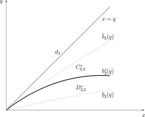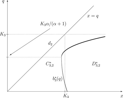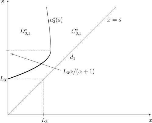holds (see Figures 1-4 below for the computer drawings of the boundary estimates ${\overline{a}}_1$, ${\underset{\_}{b}}_1$ and ${\overline{a}}_2(s)$, ${\underset{\_}{b}}_2(q)$).

(ii) Let us now describe the structure of the continuation regions in (34(34) $C_{i,1}^{\ast }=\{(x,s)\in E_1|V_i^{\ast }(x,s)>0\}$(34) ) and (35(35) $C_{i,2}^{\ast }=\{(x,q)\in E_2|U_i^{\ast }(x,q)>0\}$(35) ). For this purpose, we provide an analysis of the reward functionals of the optimal stopping problems from (25(25) $V_i^{\ast }(x,s)=\underset{\tau }{sup}{E}_{x,s}[{\int }_0^{\tau }{\mathrm{e}}^{-ru}{H}_{i,1}(X_u,S_u)\mathrm{d}u+{\int }_0^{\tau }{\mathrm{e}}^{-ru}{\mathrm{\partial }}_s{G}_i(S_u,S_u)\mathrm{d}{S}_u]$(25) ) and (26(26) $U_i^{\ast }(x,q)=\underset{\zeta }{sup}{E}_{x,q}[{\int }_0^{\zeta }{\mathrm{e}}^{-ru}{H}_{i,2}(X_u,Q_u)\mathrm{d}u+{\int }_0^{\zeta }{\mathrm{e}}^{-ru}{\mathrm{\partial }}_q{F}_i(Q_u,Q_u)\mathrm{d}{Q}_u]$(26) ). On the one hand, we observe that the function $H_{1,1}(x,s)=({\delta }^{\mathrm{\prime }}x-r{L}_1)(s/x{)}^{\alpha }$ decreases in x on the interval $(0,{\underset{\_}{a}}_1)$, and then, it increases in x on the interval $({\underset{\_}{a}}_1,s)$ with ${\underset{\_}{a}}_1=r{L}_1\alpha /({\delta }^{\mathrm{\prime }}(\alpha -1))<r{L}_1/{\delta }^{\mathrm{\prime }}={\overline{a}}_1$, under $\alpha <0$, for each $s>{\underset{\_}{s}}_1$ fixed and some $0\le {\underset{\_}{s}}_1\le {\overline{a}}_1$. In this case, the function $H_{1,1}(x,s)$ attains its global minimum at $x={\underset{\_}{a}}_1$, for any $s>{\underset{\_}{s}}_1$. According to the comparison results for strong solutions of (one-dimensional) stochastic differential equations (see, e.g. [13, Theorem 1]), this fact means that the process $(H_{1,1}(X_t,S_t){)}_{t\ge 0}$ started at the point $H_{1,1}({\underset{\_}{a}}_1,s)$ has the smallest sample paths than the one started at any other point $H_{1,1}(x,s)$, for any 0<x<s such that $x\ne {\underset{\_}{a}}_1$ and $s>{\underset{\_}{s}}_1$. In this respect, we may conclude that the point $({\underset{\_}{a}}_1,s)$ belongs to the stopping region $D_{i,1}^{\ast }$, for i = 1, which has the form: (36) $D_{i,1}^{\ast }=\{(x,s)\in E_1|V_i^{\ast }(x,s)=0\}$(36) for every i = 1, 2, 3 (see, e.g. [41, Chapter I, Subsection 2.2]), since otherwise, all the points $(x,s)$ such that 0<x<s, for any $s>{\underset{\_}{s}}_1$, would belong to the continuation region $C_{1,1}^{\ast }$ from (34(34) $C_{i,1}^{\ast }=\{(x,s)\in E_1|V_i^{\ast }(x,s)>0\}$(34) ) too. The latter fact contradicts the obvious property that it is better to stop the process $(X,S)$ at time zero than do not stop the process at all during the infinite time interval, under the assumption that $\alpha <0$. Therefore, taking into account the fact that the function $H_{1,1}(x,s)$ is negative on the interval $(0,{\underset{\_}{a}}_1)$, we see that all the points $(x,s)$ such that $0<x\le {\underset{\_}{a}}_1\wedge s$, for any $s>{\underset{\_}{s}}_1$, belong to the stopping region $D_{1,1}^{\ast }$ from (36(36) $D_{i,1}^{\ast }=\{(x,s)\in E_1|V_i^{\ast }(x,s)=0\}$(36) ) as well.

Note that similar arguments applied for the function $H_{2,1}(x,s)=({\delta }^{\mathrm{\prime }}{L}_{2}x-rs)(s/x{)}^{\alpha }$ show that all the points $(x,s)$ such that $0<x\le {\underset{\_}{a}}_2(s)\wedge s$, with ${\underset{\_}{a}}_2(s)=rs\alpha /({\delta }^{\mathrm{\prime }}{L}_2(\alpha -1))<rs/({\delta }^{\mathrm{\prime }}{L}_2)={\overline{a}}_2(s)$, under $\alpha <0$, for each $s>{\underset{\_}{s}}_2=0$ fixed, belong to the stopping region $D_{2,1}^{\ast }$ from (36(36) $D_{i,1}^{\ast }=\{(x,s)\in E_1|V_i^{\ast }(x,s)=0\}$(36) ). Moreover, it follows from the property that the function $H_{3,1}(x,s)=r(L_3-s)(s/x{)}^{\alpha }$ increases in x on the interval $(0,s)$, under $\alpha <0$, that, for each $s>{\underset{\_}{s}}_3=L_3$ fixed, there exists a sufficiently small x>0 such that the point $(x,s)$ belongs to the stopping region $D_{3,1}^{\ast }$ from (36(36) $D_{i,1}^{\ast }=\{(x,s)\in E_1|V_i^{\ast }(x,s)=0\}$(36) ). According to arguments similar to the ones applied in [9, Subsection 3.3] and [37, Subsection 3.3], the latter properties can be explained by the fact that the costs of waiting until the process X comes from such a small x>0 to the current value of the maximum S may be too high, due to the presence of the discounting factor in the reward functional of (25(25) $V_i^{\ast }(x,s)=\underset{\tau }{sup}{E}_{x,s}[{\int }_0^{\tau }{\mathrm{e}}^{-ru}{H}_{i,1}(X_u,S_u)\mathrm{d}u+{\int }_0^{\tau }{\mathrm{e}}^{-ru}{\mathrm{\partial }}_s{G}_i(S_u,S_u)\mathrm{d}{S}_u]$(25) ), one should stop at this x>0 immediately.

On the other hand, we observe that the function $H_{1,2}(x,q)=(r{K}_1-{\delta }^{\mathrm{\prime }}x)(q/x{)}^{\alpha }$ decreases in x on the interval $(q,{\overline{b}}_1)$, and then, it increases in x on the interval $({\overline{b}}_1,\mathrm{\infty })$ with ${\overline{b}}_1=r{K}_1\alpha /({\delta }^{\mathrm{\prime }}(\alpha -1))>r{K}_1/{\delta }^{\mathrm{\prime }}={\underset{\_}{b}}_1$, under $\alpha >1$, for each $q<{\overline{q}}_1$ fixed and some ${\overline{q}}_1\ge {\underset{\_}{b}}_1$. In this case, the function $H_{1,2}(x,q)$ attains its global minimum at $x={\overline{b}}_1$, for any $q<{\overline{q}}_1$. According to the comparison results for strong solutions of (one-dimensional) stochastic differential equations, this fact means that the process $(H_{1,2}(X_t,Q_t){)}_{t\ge 0}$ started at the point $H_{1,2}({\overline{b}}_1,q)$ has the smallest sample paths than the one started at any other point $H_{1,2}(x,q)$, for any x>q such that $x\ne {\overline{b}}_1$ and $q<{\overline{q}}_1$. In this respect, we may conclude that the point $({\overline{b}}_1,q)$ belongs to the stopping region $D_{i,2}^{\ast }$, for i = 1, which has the form: (37) $D_{i,2}^{\ast }=\{(x,q)\in E_2|U_i^{\ast }(x,q)=0\}$(37) for i = 1, 2, 3, respectively, since otherwise, all the points $(x,q)$ such that x>q, for any $q<{\overline{q}}_1$, would belong to the continuation region $C_{1,2}^{\ast }$ from (35(35) $C_{i,2}^{\ast }=\{(x,q)\in E_2|U_i^{\ast }(x,q)>0\}$(35) ) too. The latter fact contradicts the obvious property that it is better to stop the process $(X,Q)$ at time zero than do not stop the process at all during the infinite time interval, under the assumption that $\alpha >1$. Therefore, taking into account the fact that the function $H_{1,2}(x,q)$ is negative on the interval $({\overline{b}}_1,\mathrm{\infty })$, we see that all the points $(x,q)$ such that $x\ge {\overline{b}}_1\vee q$, for any $q<{\overline{q}}_1$, belong to the stopping region $D_{1,2}^{\ast }$ from (37(37) $D_{i,2}^{\ast }=\{(x,q)\in E_2|U_i^{\ast }(x,q)=0\}$(37) ) as well.

Note that similar arguments applied for the function $H_{2,2}(x,q)=(rq-{\delta }^{\mathrm{\prime }}{K}_{2}x)(q/x{)}^{\alpha }$ show that all the points $(x,q)$ such that $x\ge {\overline{b}}_2(q)\vee q$, with ${\overline{b}}_2(q)=rq\alpha /({\delta }^{\mathrm{\prime }}{K}_2(\alpha -1))>rq/({\delta }^{\mathrm{\prime }}{K}_2)={\underset{\_}{b}}_2(q)$, under $\alpha >1$, for each $q<{\overline{q}}_2=\mathrm{\infty }$ fixed, belong to the stopping region $D_{2,2}^{\ast }$ from (37(37) $D_{i,2}^{\ast }=\{(x,q)\in E_2|U_i^{\ast }(x,q)=0\}$(37) ). Moreover, it follows from the fact that the function $H_{3,2}(x,q)=r(q-K_3)(q/x{)}^{\alpha }$ is strictly increasing in x on the interval $(q,\mathrm{\infty })$, under $\alpha >0$, that, for each $q<{\overline{q}}_3=K_3$ fixed, there exists a sufficiently large x>0 such that the point $(x,q)$ belongs to the stopping region $D_{3,2}^{\ast }$ from (37(37) $D_{i,2}^{\ast }=\{(x,q)\in E_2|U_i^{\ast }(x,q)=0\}$(37) ). The same arguments based on the strict increase of the functions $H_{i,2}(x,q)$, for i = 1, 2, in x on the interval $(q,\mathrm{\infty })$, under $0<\alpha \le 1$, for each $q<{\overline{q}}_i$ fixed, for i = 1, 2, with some ${\overline{q}}_1>{\underset{\_}{b}}_1$ and ${\overline{q}}_2=\mathrm{\infty }$, show that, there exists a sufficiently large x>0 such that the point $(x,q)$ belongs to the stopping regions $D_{i,2}^{\ast }$, for i = 1, 2, from (37(37) $D_{i,2}^{\ast }=\{(x,q)\in E_2|U_i^{\ast }(x,q)=0\}$(37) ). The latter properties can be explained by the fact that the costs of waiting until the process X comes from such a large x>0 to the current value of the minimum Q may be too high, due to the presence of the discounting factor in the reward functional of (26(26) $U_i^{\ast }(x,q)=\underset{\zeta }{sup}{E}_{x,q}[{\int }_0^{\zeta }{\mathrm{e}}^{-ru}{H}_{i,2}(X_u,Q_u)\mathrm{d}u+{\int }_0^{\zeta }{\mathrm{e}}^{-ru}{\mathrm{\partial }}_q{F}_i(Q_u,Q_u)\mathrm{d}{Q}_u]$(26) ), one should stop at this x>0 immediately. In this view, we can set ${\overline{b}}_1=\mathrm{\infty }$ and ${\overline{b}}_2(q)=\mathrm{\infty }$, for q>0, under $0<\alpha \le 1$ (see Figures 1–4 below for the computer drawings of the boundary estimates ${\underset{\_}{a}}_1$, ${\overline{b}}_1$ and ${\underset{\_}{a}}_2(s)$, ${\overline{b}}_2(q)$).

Figure 1. A computer drawing of the continuation and stopping regions $C_{1,1}^{\ast }$ and $D_{1,1}^{\ast }$ formed by the optimal exercise boundary $a_1^{\ast }(s)$ and its estimates ${\underset{\_}{a}}_1$ and ${\overline{a}}_1$.

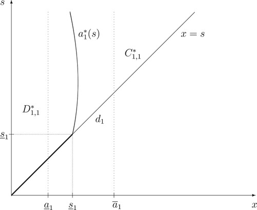
Figure 2. A computer drawing of the continuation and stopping regions $C_{1,2}^{\ast }$ and $D_{1,2}^{\ast }$ formed by the optimal exercise boundary $b_1^{\ast }(s)$ and its estimates ${\underset{\_}{b}}_1$ and ${\overline{b}}_1$.

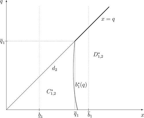
Figure 3. A computer drawing of the continuation and stopping regions $C_{2,1}^{\ast }$ and $D_{2,1}^{\ast }$ formed by the optimal exercise boundary $a_2^{\ast }(s)$ and its estimates ${\underset{\_}{a}}_2(s)$ and ${\overline{a}}_2(s)$.

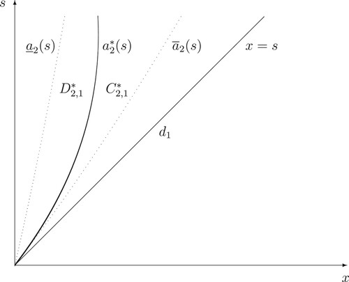
Figure 4. A computer drawing of the continuation and stopping regions $C_{2,2}^{\ast }$ and $D_{2,2}^{\ast }$ formed by the optimal exercise boundary $b_2^{\ast }(q)$ and its estimates ${\underset{\_}{b}}_2(q)$ and ${\overline{b}}_2(q)$.

It is seen from the results of Theorem 4.1 proved below that the value functions $V_i^{\ast }(x,s)$ and $U_i^{\ast }(x,q)$ are continuous, so that the sets $C_{i,1}^{\ast }$ and $C_{i,2}^{\ast }$ in (34(34) $C_{i,1}^{\ast }=\{(x,s)\in E_1|V_i^{\ast }(x,s)>0\}$(34) ) and (35(35) $C_{i,2}^{\ast }=\{(x,q)\in E_2|U_i^{\ast }(x,q)>0\}$(35) ) are open, while the sets $D_{i,1}^{\ast }$ and $D_{i,2}^{\ast }$ in (36(36) $D_{i,1}^{\ast }=\{(x,s)\in E_1|V_i^{\ast }(x,s)=0\}$(36) ) and (37(37) $D_{i,2}^{\ast }=\{(x,q)\in E_2|U_i^{\ast }(x,q)=0\}$(37) ) are closed, for every i = 1, 2, 3 (see Figures 1–6 for the computer drawings of the continuation and stopping regions $C_{i,j}^{\ast }$ and $D_{i,j}^{\ast }$, for i = 1, 2, 3 and j = 1, 2).

Figure 6. A computer drawing of the continuation and stopping regions $C_{3,2}^{\ast }$ and $D_{3,2}^{\ast }$ formed by the optimal exercise boundary $b_3^{\ast }(q)$ and the points $K_3$ and $K_3\alpha /(\alpha +1)$.

(iii) Now, we observe that, if we take some $(x,s)\in D_{i,1}^{\ast }$ from (36(36) $D_{i,1}^{\ast }=\{(x,s)\in E_1|V_i^{\ast }(x,s)=0\}$(36) ) such that $x>{\underset{\_}{a}}_i(s)$ with ${\underset{\_}{a}}_i(s)$ specified above and use the fact that the process $(X,S)$ started at some $(x^{\mathrm{\prime }},s)$ such that ${\underset{\_}{a}}_i(s)\le x^{\mathrm{\prime }}<x$ passes through the point $(x,s)$ before hitting the diagonal $d_1=\{(x,s)\in E_1|x=s\}$, then the equality in (25(25) $V_i^{\ast }(x,s)=\underset{\tau }{sup}{E}_{x,s}[{\int }_0^{\tau }{\mathrm{e}}^{-ru}{H}_{i,1}(X_u,S_u)\mathrm{d}u+{\int }_0^{\tau }{\mathrm{e}}^{-ru}{\mathrm{\partial }}_s{G}_i(S_u,S_u)\mathrm{d}{S}_u]$(25) ) implies that $V_i^{\ast }(x^{\mathrm{\prime }},s)\le V_i^{\ast }(x,s)=0$ holds, so that $(x^{\mathrm{\prime }},s)\in D_{i,1}^{\ast }$, for i = 1, 2, 3. Moreover, if we take some $(x,q)\in D_{i,2}^{\ast }$ from (37(37) $D_{i,2}^{\ast }=\{(x,q)\in E_2|U_i^{\ast }(x,q)=0\}$(37) ) such that $x<{\overline{b}}_i(q)$ with ${\overline{b}}_i(q)$ specified above and use the fact that the process $(X,Q)$ started at some $(x^{\mathrm{\prime }},q)$ such that ${\overline{b}}_i(q)\ge x^{\mathrm{\prime }}>x$ passes through the point $(x,q)$ before hitting the diagonal $d_2=\{(x,q)\in E_2|x=q\}$, then the equality in (26(26) $U_i^{\ast }(x,q)=\underset{\zeta }{sup}{E}_{x,q}[{\int }_0^{\zeta }{\mathrm{e}}^{-ru}{H}_{i,2}(X_u,Q_u)\mathrm{d}u+{\int }_0^{\zeta }{\mathrm{e}}^{-ru}{\mathrm{\partial }}_q{F}_i(Q_u,Q_u)\mathrm{d}{Q}_u]$(26) ) implies that $U_i^{\ast }(x^{\mathrm{\prime }},q)\le U_i^{\ast }(x,q)=0$ holds, so that $(x^{\mathrm{\prime }},q)\in D_{i,2}^{\ast }$, for i = 1, 2, 3.

On the other hand, if take some $(x,s)\in C_{i,1}^{\ast }$ from (34(34) $C_{i,1}^{\ast }=\{(x,s)\in E_1|V_i^{\ast }(x,s)>0\}$(34) ) and use the fact that the process $(X,S)$ started at $(x,s)$ passes through some point $(x^{\mathrm{\prime }\mathrm{\prime }},s)$ such that $x^{\mathrm{\prime }\mathrm{\prime }}>x$ before hitting the diagonal $d_1$, then the equality in (25(25) $V_i^{\ast }(x,s)=\underset{\tau }{sup}{E}_{x,s}[{\int }_0^{\tau }{\mathrm{e}}^{-ru}{H}_{i,1}(X_u,S_u)\mathrm{d}u+{\int }_0^{\tau }{\mathrm{e}}^{-ru}{\mathrm{\partial }}_s{G}_i(S_u,S_u)\mathrm{d}{S}_u]$(25) ) yields that $V_i^{\ast }(x^{\mathrm{\prime }\mathrm{\prime }},s)\ge V_i^{\ast }(x,s)>0$ holds, so that $(x^{\mathrm{\prime }\mathrm{\prime }},s)\in C_{i,1}^{\ast }$, for i = 1, 2, 3. Moreover, if we take some $(x,q)\in C_{i,2}^{\ast }$ from (35(35) $C_{i,2}^{\ast }=\{(x,q)\in E_2|U_i^{\ast }(x,q)>0\}$(35) ) and use the fact that the process $(X,Q)$ started at $(x,q)$ passes through some point $(x^{\mathrm{\prime }\mathrm{\prime }},q)$ such that $x^{\mathrm{\prime }\mathrm{\prime }}<x$ before hitting the diagonal $d_2$, then the equality in (26(26) $U_i^{\ast }(x,q)=\underset{\zeta }{sup}{E}_{x,q}[{\int }_0^{\zeta }{\mathrm{e}}^{-ru}{H}_{i,2}(X_u,Q_u)\mathrm{d}u+{\int }_0^{\zeta }{\mathrm{e}}^{-ru}{\mathrm{\partial }}_q{F}_i(Q_u,Q_u)\mathrm{d}{Q}_u]$(26) ) yields that $U_i^{\ast }(x^{\mathrm{\prime }\mathrm{\prime }},q)\ge U_i^{\ast }(x,q)>0$ holds, so that $(x^{\mathrm{\prime }\mathrm{\prime }},q)\in C_{i,2}^{\ast }$.

Hence, we may conclude that there exist functions $a_i^{\ast }(s)$ and $b_i^{\ast }(q)$ satisfying the inequalities $a_i^{\ast }(s)<{\overline{a}}_i(s)\wedge s$, for all $s>{\underset{\_}{s}}_i$, and $b_i^{\ast }(q)>{\underset{\_}{b}}_i(q)\vee q$, for all $q<{\overline{q}}_i$, as well as the equalities $a_1^{\ast }(s)=s$, $a_3^{\ast }(s)=0$, for all $s\le {\underset{\_}{s}}_i$, and $b_1^{\ast }(q)=q$, $b_3^{\ast }(q)=\mathrm{\infty }$, for all $q\ge {\overline{q}}_i$, such that the continuation regions $C_{i,j}^{\ast }$, for $j=1,2$, in (34(34) $C_{i,1}^{\ast }=\{(x,s)\in E_1|V_i^{\ast }(x,s)>0\}$(34) ) and (35(35) $C_{i,2}^{\ast }=\{(x,q)\in E_2|U_i^{\ast }(x,q)>0\}$(35) ) have the form: (38) $C_{i,1}^{\ast }=\{(x,s)\in E_1|a_i^{\ast }(s)<x\le s\}\mathrm{and}{C}_{i,2}^{\ast }=\{(x,q)\in E_2|q\le x<b_i^{\ast }(q)\}$(38) while the stopping regions $D_{i,j}^{\ast }$, for j = 1, 2, in (36(36) $D_{i,1}^{\ast }=\{(x,s)\in E_1|V_i^{\ast }(x,s)=0\}$(36) ) and (37(37) $D_{i,2}^{\ast }=\{(x,q)\in E_2|U_i^{\ast }(x,q)=0\}$(37) ) are given by: (39) $D_{i,1}^{\ast }=\{(x,s)\in E_1|x\le a_i^{\ast }(s)\}\mathrm{and}{D}_{i,2}^{\ast }=\{(x,q)\in E_2|x\ge b_i^{\ast }(q)\}$(39) for every i = 1, 2, 3, respectively (see Figures 1–6 for the computer drawings of the optimal stopping boundaries $a_i^{\ast }(s)$ and $b_i^{\ast }(q)$, for i = 1, 2, 3).

(iv) We finally specify the behaviour of the optimal exercise boundaries $a_3^{\ast }(s)$ and $b_3^{\ast }(q)$. For the ease of presentation, in the rest of this section, we indicate by $(X^{(x)},S^{(s,x)})$ and $(X^{(x)},Q^{(q,x)})$ the dependence of the processes $(X,S)$ and $(X,Q)$ defined in (1(1) $X_t=x\exp ((r-\delta -{\sigma }^2/2)t+\sigma B_t)$(1) ) and (5(5) $S_t=s\vee \left(\underset{0\le u\le t}{max}{X}_u\right)\mathrm{and}{Q}_t=q\wedge \left(\underset{0\le u\le t}{min}{X}_u\right)$(5) ) from their starting points $(x,s)\in E_1$ and $(x,q)\in E_2$. Let us first fix some $(x,s)\in C_{3,1}^{\ast }$ such that $L_3={\underset{\_}{s}}_3<s<L_3\alpha /(\alpha +1)$, under $\alpha <-1$, so that $V_3^{\ast }(x,s)>0$ holds. Then, consider the optimal stopping time ${\tau }_3^{\ast }={\tau }_3^{\ast }(x,s)$ for the problem (25(25) $V_i^{\ast }(x,s)=\underset{\tau }{sup}{E}_{x,s}[{\int }_0^{\tau }{\mathrm{e}}^{-ru}{H}_{i,1}(X_u,S_u)\mathrm{d}u+{\int }_0^{\tau }{\mathrm{e}}^{-ru}{\mathrm{\partial }}_s{G}_i(S_u,S_u)\mathrm{d}{S}_u]$(25) ), for i = 3, for this starting point $(x,s)$ of the process $(X,S)$ from (1(1) $X_t=x\exp ((r-\delta -{\sigma }^2/2)t+\sigma B_t)$(1) ) and (5(5) $S_t=s\vee \left(\underset{0\le u\le t}{max}{X}_u\right)\mathrm{and}{Q}_t=q\wedge \left(\underset{0\le u\le t}{min}{X}_u\right)$(5) ). Then, using the property that the function $H_{3,1}(x,s)=r(L_3-s)(s/x{)}^{\alpha }$ is decreasing in s on $(L_3,L_3\alpha /(\alpha +1))$, under $\alpha <-1$, for each x>0 fixed, and the fact that ${\mathrm{\partial }}_s{G}_3(s,s)=1$, by virtue of the structure of the running maximum $S^{(s,x)}$ of the process $X^{(x)}$, for any other starting point $(x,s^{\mathrm{\prime }})\in E_1$ such that $L_3<s^{\mathrm{\prime }}<s<L_3\alpha /(\alpha +1)$, we have: (40) $\begin{array}{rl}{V}_3^{\ast }(x,s^{\mathrm{\prime }})& \ge E[{\int }_0^{{\tau }_3^{\ast }}{\mathrm{e}}^{-ru}{H}_{3,1}(X_u^{(x)},S_u^{(s^{\mathrm{\prime }},x)})\mathrm{d}u+{\int }_0^{{\tau }_3^{\ast }}{\mathrm{e}}^{-ru}\mathrm{d}{S}_u^{(s^{\mathrm{\prime }},x)}]\\ & \ge E[{\int }_0^{{\tau }_3^{\ast }}{\mathrm{e}}^{-ru}{H}_{3,1}(X_u^{(x)},S_u^{(s,x)})\mathrm{d}u+{\int }_0^{{\tau }_3^{\ast }}{\mathrm{e}}^{-ru}\mathrm{d}{S}_u^{(s,x)}]=V_3^{\ast }(x,s)>0\end{array}$(40) so that $(x,s^{\mathrm{\prime }})\in C_{3,1}^{\ast }$ too. Thus, we may conclude that the left-hand boundary $a_3^{\ast }(s)$ is increasing on $(L_3,L_3\alpha /(\alpha +1))$, under $\alpha <-1$. Moreover, for any starting point $(x,s)\in C_{3,1}^{\ast }$ such that $s>{\underset{\_}{s}}_3=L_3$, using the fact that the function $H_{3,1}(x,s)$ is decreasing in s on $(L_3,\mathrm{\infty })$, under $-1\le \alpha <0$, for each x>0 fixed, by means of arguments similar to the ones used above, we may conclude that $V_3^{\ast }(x,s^{\mathrm{\prime }})\ge V_3^{\ast }(x,s)>0$ holds, for all $s>s^{\mathrm{\prime }}>L_3$, and thus, we have $(x,s^{\mathrm{\prime }})\in C_{3,1}^{\ast }$, and the boundary $a_3^{\ast }(s)$ is increasing on $(L_3,\mathrm{\infty })$, under $-1\le \alpha <0$.

Let us now fix some $(x,q)\in C_{3,2}^{\ast }$ such that $K_3\alpha /(\alpha +1)<q<{\overline{q}}_3=K_3$, under $\alpha >0$, so that $U_3^{\ast }(x,q)>0$ holds. Then, using the fact that the function $H_{3,2}(x,q)=r(q-K_3)(q/x{)}^{\alpha }$ is increasing in q on $(K_3\alpha /(\alpha +1),K_3)$, under $\alpha >0$, for each x>0 fixed, by virtue of the structure of the running minimum $Q^{(q,x)}$ of the process $X^{(x)}$, for any other starting point $(x,q^{\mathrm{\prime }})\in E_2$ such that $K_3<q<q^{\mathrm{\prime }}<K_3\alpha /(\alpha +1)$, we have: (41) $\begin{array}{rl}{U}_3^{\ast }(x,q^{\mathrm{\prime }})& \ge E[{\int }_0^{{\zeta }_3^{\ast }}{\mathrm{e}}^{-ru}{H}_{3,2}(X_u^{(x)},Q_u^{(q^{\mathrm{\prime }},x)})\mathrm{d}u-{\int }_0^{{\zeta }_3^{\ast }}{\mathrm{e}}^{-ru}\mathrm{d}{Q}_u^{(q^{\mathrm{\prime }},x)}]\\ & \ge E[{\int }_0^{{\zeta }_3^{\ast }}{\mathrm{e}}^{-ru}{H}_{3,2}(X_u^{(x)},Q_u^{(q,x)})\mathrm{d}u-{\int }_0^{{\zeta }_3^{\ast }}{\mathrm{e}}^{-ru}\mathrm{d}{Q}_u^{(q,x)}]=U_3^{\ast }(x,q)>0\end{array}$(41) so that $(x,q^{\mathrm{\prime }})\in C_{3,2}^{\ast }$ too. Thus, we may conclude that the right-hand boundary $b_3^{\ast }(q)$ is increasing on $(K_3\alpha /(\alpha +1),K_3)$, under $\alpha >0$ (see Figures 5 and 6 for the computer drawings of locations of the optimal stopping boundaries $a_3^{\ast }(s)$ and $b_3^{\ast }(q)$ with respect to the points $L_3$, $L_3\alpha /(\alpha +1)$ and $K_3$, $K_3\alpha /(\alpha +1)$).

Figure 5. A computer drawing of the continuation and stopping regions $C_{3,1}^{\ast }$ and $D_{3,1}^{\ast }$ formed by the optimal exercise boundary $a_3^{\ast }(s)$ and the points $L_3$ and $L_3\alpha /(\alpha +1)$.

2.3. The free-boundary problems

By means of standard arguments based on the application of Itô's formula, it is shown that the infinitesimal operator $\mathbb{L}$ of the process $(X,S)$ or $(X,Q)$ from (2(2) $\mathrm{d}{X}_t=(r-\delta )X_t\mathrm{d}t+\sigma X_t\mathrm{d}{B}_t(X_0=x)$(2) ) and (5(5) $S_t=s\vee \left(\underset{0\le u\le t}{max}{X}_u\right)\mathrm{and}{Q}_t=q\wedge \left(\underset{0\le u\le t}{min}{X}_u\right)$(5) ) has the form: (42) $\begin{array}{rl}& \mathbb{L}=(r-\delta )x{\mathrm{\partial }}_x+\frac{{\sigma }^2{x}^2}{2}{\mathrm{\partial }}_{xx}\mathrm{in}0<x<s\mathrm{or}0<q<x\end{array}$(42) (43) $\begin{array}{rl}& {\mathrm{\partial }}_s=0\mathrm{at}0<x=s\mathrm{or}{\mathrm{\partial }}_q=0\mathrm{at}0<x=q\end{array}$(43) (see, e.g. [37, Subsection 3.1]). In order to find analytic expressions for the unknown value functions $V_i^{\ast }(x,s)$ and $U_i^{\ast }(x,q)$ from (25(25) $V_i^{\ast }(x,s)=\underset{\tau }{sup}{E}_{x,s}[{\int }_0^{\tau }{\mathrm{e}}^{-ru}{H}_{i,1}(X_u,S_u)\mathrm{d}u+{\int }_0^{\tau }{\mathrm{e}}^{-ru}{\mathrm{\partial }}_s{G}_i(S_u,S_u)\mathrm{d}{S}_u]$(25) ) and (26(26) $U_i^{\ast }(x,q)=\underset{\zeta }{sup}{E}_{x,q}[{\int }_0^{\zeta }{\mathrm{e}}^{-ru}{H}_{i,2}(X_u,Q_u)\mathrm{d}u+{\int }_0^{\zeta }{\mathrm{e}}^{-ru}{\mathrm{\partial }}_q{F}_i(Q_u,Q_u)\mathrm{d}{Q}_u]$(26) ) and the unknown boundaries $a_i^{\ast }(s)$ and $b_i^{\ast }(q)$ from (38(38) $C_{i,1}^{\ast }=\{(x,s)\in E_1|a_i^{\ast }(s)<x\le s\}\mathrm{and}{C}_{i,2}^{\ast }=\{(x,q)\in E_2|q\le x<b_i^{\ast }(q)\}$(38) ) and (39(39) $D_{i,1}^{\ast }=\{(x,s)\in E_1|x\le a_i^{\ast }(s)\}\mathrm{and}{D}_{i,2}^{\ast }=\{(x,q)\in E_2|x\ge b_i^{\ast }(q)\}$(39) ), for every i = 1, 2, 3, we apply the results of general theory for solving optimal stopping problems for Markov processes presented in [41, Chapter IV, Section 8] among others (see also [41, Chapter V, Sections 15-20] for optimal stopping problems for maxima processes and other related references). More precisely, for the original optimal stopping problems in (25(25) $V_i^{\ast }(x,s)=\underset{\tau }{sup}{E}_{x,s}[{\int }_0^{\tau }{\mathrm{e}}^{-ru}{H}_{i,1}(X_u,S_u)\mathrm{d}u+{\int }_0^{\tau }{\mathrm{e}}^{-ru}{\mathrm{\partial }}_s{G}_i(S_u,S_u)\mathrm{d}{S}_u]$(25) ) and (26(26) $U_i^{\ast }(x,q)=\underset{\zeta }{sup}{E}_{x,q}[{\int }_0^{\zeta }{\mathrm{e}}^{-ru}{H}_{i,2}(X_u,Q_u)\mathrm{d}u+{\int }_0^{\zeta }{\mathrm{e}}^{-ru}{\mathrm{\partial }}_q{F}_i(Q_u,Q_u)\mathrm{d}{Q}_u]$(26) ), we formulate the associated free-boundary problems (see, e.g. [41, Chapter IV, Section 8]) and then verify in Theorem 4.1 below that the appropriate candidate solutions of the latter problems coincide with the solutions of the original problems. In other words, we reduce the optimal stopping problems of (25(25) $V_i^{\ast }(x,s)=\underset{\tau }{sup}{E}_{x,s}[{\int }_0^{\tau }{\mathrm{e}}^{-ru}{H}_{i,1}(X_u,S_u)\mathrm{d}u+{\int }_0^{\tau }{\mathrm{e}}^{-ru}{\mathrm{\partial }}_s{G}_i(S_u,S_u)\mathrm{d}{S}_u]$(25) ) and (26(26) $U_i^{\ast }(x,q)=\underset{\zeta }{sup}{E}_{x,q}[{\int }_0^{\zeta }{\mathrm{e}}^{-ru}{H}_{i,2}(X_u,Q_u)\mathrm{d}u+{\int }_0^{\zeta }{\mathrm{e}}^{-ru}{\mathrm{\partial }}_q{F}_i(Q_u,Q_u)\mathrm{d}{Q}_u]$(26) ) to the following equivalent free-boundary problems: (44) $\begin{array}{rl}& (\mathbb{L}{V}_i-r{V}_i)(x,s)=-H_{i,1}(x,s)\mathrm{for}(x,s)\in C_{i,1}\setminus \{(x,s)\in E_1|x=s\}\end{array}$(44) (45) $\begin{array}{rl}& (\mathbb{L}{U}_i-r{U}_i)(x,q)=-H_{i,2}(x,q)\mathrm{for}(x,q)\in C_{i,2}\setminus \{(x,q)\in E_2|x=q\}\end{array}$(45) (46) $\begin{array}{rl}& V_i(x,s){|}_{x=a_i(s)+}=0\mathrm{and}{U}_i(x,q){|}_{x=b_i(q)-}=0\end{array}$(46) (47) $\begin{array}{rl}& {\mathrm{\partial }}_x{V}_i(x,s){|}_{x=a_i(s)+}=0\mathrm{and}{\mathrm{\partial }}_x{U}_i(x,q){|}_{x=b_i(q)-}=0\end{array}$(47) (48) $\begin{array}{rl}& {\mathrm{\partial }}_s{V}_i(x,s){|}_{x=s-}=-{\mathrm{\partial }}_s{G}_i(s,s)\mathrm{and}{\mathrm{\partial }}_q{U}_i(x,q){|}_{x=q+}=-{\mathrm{\partial }}_q{F}_i(q,q)\end{array}$(48) (49) $\begin{array}{rl}& V_i(x,s)=0\mathrm{for}(x,s)\in D_{i,1}\mathrm{and}{U}_i(x,q)=0\mathrm{for}(x,q)\in D_{i,2}\end{array}$(49) (50) $\begin{array}{rl}& V_i(x,s)>0\mathrm{for}(x,s)\in C_{i,1}\mathrm{and}{U}_i(x,q)>0\mathrm{for}(x,q)\in C_{i,2}\end{array}$(50) (51) $\begin{array}{rl}& (\mathbb{L}{V}_i-r{V}_i)(x,s)<-H_{i,1}(x,s)\mathrm{for}(x,s)\in D_{i,1}\end{array}$(51) (52) $\begin{array}{rl}& (\mathbb{L}{U}_i-r{U}_i)(x,q)<-H_{i,2}(x,q)\mathrm{for}(x,q)\in D_{i,2}\end{array}$(52) where $C_{i,j}$ and $D_{i,j}$ are defined as $C_{i,j}^{\ast }$ and $D_{i,j}^{\ast }$, for j = 1, 2, in (38(38) $C_{i,1}^{\ast }=\{(x,s)\in E_1|a_i^{\ast }(s)<x\le s\}\mathrm{and}{C}_{i,2}^{\ast }=\{(x,q)\in E_2|q\le x<b_i^{\ast }(q)\}$(38) ) and (39(39) $D_{i,1}^{\ast }=\{(x,s)\in E_1|x\le a_i^{\ast }(s)\}\mathrm{and}{D}_{i,2}^{\ast }=\{(x,q)\in E_2|x\ge b_i^{\ast }(q)\}$(39) ) with the unknown functions $a_i(s)$ and $b_i(q)$ instead of $a_i^{\ast }(s)$ and $b_i^{\ast }(q)$, where the functions $H_{i,1}(x,s)$ and $H_{i,2}(x,q)$, for every i = 1, 2, 3, are defined in (23(23) $H_{i,1}(x,s)=({\mathrm{\partial }}_x{G}_i(x,s)(r-{\delta }^{\mathrm{\prime }})x-r{G}_i(x,s))(s/x{)}^{\alpha }$(23) ) and (24(24) $H_{i,2}(x,q)=({\mathrm{\partial }}_x{F}_i(x,q)(r-{\delta }^{\mathrm{\prime }})x-r{F}_i(x,q))(q/x{)}^{\alpha }$(24) ), respectively. Here, the instantaneous-stopping as well as the smooth-fit and normal-reflection conditions of (46(46) $\begin{array}{rl}& V_i(x,s){|}_{x=a_i(s)+}=0\mathrm{and}{U}_i(x,q){|}_{x=b_i(q)-}=0\end{array}$(46) )–(48(48) $\begin{array}{rl}& {\mathrm{\partial }}_s{V}_i(x,s){|}_{x=s-}=-{\mathrm{\partial }}_s{G}_i(s,s)\mathrm{and}{\mathrm{\partial }}_q{U}_i(x,q){|}_{x=q+}=-{\mathrm{\partial }}_q{F}_i(q,q)\end{array}$(48) ) are satisfied, for all $s>{\underset{\_}{s}}_i$ and $q<{\overline{q}}_i$, for i = 1, 2, 3, with some $0\le {\underset{\_}{s}}_1\le {\overline{a}}_1=r{L}_1/{\delta }^{\mathrm{\prime }}$ and ${\overline{q}}_1\ge {\underset{\_}{b}}_1=r{K}_1/{\delta }^{\mathrm{\prime }}$, as well as ${\underset{\_}{s}}_2=0$, ${\underset{\_}{s}}_3=L_3$ and ${\overline{q}}_2=\mathrm{\infty }$, ${\overline{q}}_3=K_3$. Observe that the superharmonic characterization of the value function (see, e.g. [41, Chapter IV, Section 9]) implies that $V_i^{\ast }(x,s)$ and $U_i^{\ast }(x,q)$ are the smallest functions satisfying (44(44) $\begin{array}{rl}& (\mathbb{L}{V}_i-r{V}_i)(x,s)=-H_{i,1}(x,s)\mathrm{for}(x,s)\in C_{i,1}\setminus \{(x,s)\in E_1|x=s\}\end{array}$(44) )–(46(46) $\begin{array}{rl}& V_i(x,s){|}_{x=a_i(s)+}=0\mathrm{and}{U}_i(x,q){|}_{x=b_i(q)-}=0\end{array}$(46) ) and (49(49) $\begin{array}{rl}& V_i(x,s)=0\mathrm{for}(x,s)\in D_{i,1}\mathrm{and}{U}_i(x,q)=0\mathrm{for}(x,q)\in D_{i,2}\end{array}$(49) )–(50(50) $\begin{array}{rl}& V_i(x,s)>0\mathrm{for}(x,s)\in C_{i,1}\mathrm{and}{U}_i(x,q)>0\mathrm{for}(x,q)\in C_{i,2}\end{array}$(50) ) with the boundaries $a_i^{\ast }(s)$ and $b_i^{\ast }(q)$, for every i = 1, 2, 3, respectively. Note that the inequalities in (51(51) $\begin{array}{rl}& (\mathbb{L}{V}_i-r{V}_i)(x,s)<-H_{i,1}(x,s)\mathrm{for}(x,s)\in D_{i,1}\end{array}$(51) ) and (52(52) $\begin{array}{rl}& (\mathbb{L}{U}_i-r{U}_i)(x,q)<-H_{i,2}(x,q)\mathrm{for}(x,q)\in D_{i,2}\end{array}$(52) ) follow directly from the arguments of parts (ii)–(iii) of Subsection 2.2 above.

3. Solutions to the free-boundary problems

In this section, we obtain solutions to the free-boundary problems in (44(44) $\begin{array}{rl}& (\mathbb{L}{V}_i-r{V}_i)(x,s)=-H_{i,1}(x,s)\mathrm{for}(x,s)\in C_{i,1}\setminus \{(x,s)\in E_1|x=s\}\end{array}$(44) )–(52(52) $\begin{array}{rl}& (\mathbb{L}{U}_i-r{U}_i)(x,q)<-H_{i,2}(x,q)\mathrm{for}(x,q)\in D_{i,2}\end{array}$(52) ) and derive first-order nonlinear ordinary differential equations for the candidate optimal stopping boundaries.

3.1. The candidate value functions

It is shown that the second-order ordinary differential equations in (44(44) $\begin{array}{rl}& (\mathbb{L}{V}_i-r{V}_i)(x,s)=-H_{i,1}(x,s)\mathrm{for}(x,s)\in C_{i,1}\setminus \{(x,s)\in E_1|x=s\}\end{array}$(44) ) and (45(45) $\begin{array}{rl}& (\mathbb{L}{U}_i-r{U}_i)(x,q)=-H_{i,2}(x,q)\mathrm{for}(x,q)\in C_{i,2}\setminus \{(x,q)\in E_2|x=q\}\end{array}$(45) ) have the general solutions: (53) $V_i(x,s)=C_{i,1}(s)x^{{\gamma }_1}+C_{i,2}(s)x^{{\gamma }_2}+A_{i,1}(s)x^{1-\alpha }{s}^{\alpha }+A_{i,2}(s)x^{-\alpha }{s}^{\alpha }$(53) when $\alpha <0$, for $0<x\le s$, and (54) $U_i(x,q)=D_{i,1}(q)x^{{\gamma }_1}+D_{i,2}(q)x^{{\gamma }_2}+B_{i,1}(q)x^{1-\alpha }{q}^{\alpha }+B_{i,2}(q)x^{-\alpha }{q}^{\alpha }$(54) when $\alpha >0$, for $0<q\le x$, respectively. Here, $C_{i,j}(s)$ and $D_{i,j}(q)$, for $i=1,2,3$ and j = 1, 2, are some arbitrary (continuously differentiable) functions, and ${\gamma }_j$, for j = 1, 2, are given by: (55) ${\gamma }_j=\frac{1}{2}-\frac{r-\delta }{{\sigma }^2}-(-1{)}^j\sqrt{{(\frac{1}{2}-\frac{r-\delta }{{\sigma }^2})}^2+\frac{2r}{{\sigma }^2}}$(55) so that ${\gamma }_2<0<1<{\gamma }_1$ holds. The functions $A_{i,j}(s)$ and $B_{i,j}(q)$, for $i=1,2,3$ and j = 1, 2, are specified by $A_{1,1}(s)=1$, $A_{1,2}(s)=-L_1$, $A_{2,1}(s)=L_2$, $A_{2,2}(s)=-s$, $A_{3,1}(s)=0$, $A_{3,2}(s)=L_3-s$, and $B_{1,1}(q)=-1$, $B_{1,2}(q)=K_1$, $B_{2,1}(q)=-K_2$, $B_{2,2}(q)=q$, $B_{3,1}(q)=0$, $B_{3,2}(q)=q-K_3$. Then, by applying the conditions of (46(46) $\begin{array}{rl}& V_i(x,s){|}_{x=a_i(s)+}=0\mathrm{and}{U}_i(x,q){|}_{x=b_i(q)-}=0\end{array}$(46) )–(48(48) $\begin{array}{rl}& {\mathrm{\partial }}_s{V}_i(x,s){|}_{x=s-}=-{\mathrm{\partial }}_s{G}_i(s,s)\mathrm{and}{\mathrm{\partial }}_q{U}_i(x,q){|}_{x=q+}=-{\mathrm{\partial }}_q{F}_i(q,q)\end{array}$(48) ) to the functions in (53(53) $V_i(x,s)=C_{i,1}(s)x^{{\gamma }_1}+C_{i,2}(s)x^{{\gamma }_2}+A_{i,1}(s)x^{1-\alpha }{s}^{\alpha }+A_{i,2}(s)x^{-\alpha }{s}^{\alpha }$(53) ) and (54(54) $U_i(x,q)=D_{i,1}(q)x^{{\gamma }_1}+D_{i,2}(q)x^{{\gamma }_2}+B_{i,1}(q)x^{1-\alpha }{q}^{\alpha }+B_{i,2}(q)x^{-\alpha }{q}^{\alpha }$(54) ), we obtain the equalities: (56) $\begin{array}{rl}& C_{i,1}(s)a_i^{{\gamma }_1}(s)+C_{i,2}(s)a_i^{{\gamma }_2}(s)+A_{i,1}(s)a_i^{1-\alpha }(s)s^{\alpha }+A_{i,2}(s)a_i^{-\alpha }(s)s^{\alpha }=0\end{array}$(56) (57) $\begin{array}{rl}& {\gamma }_1{C}_{i,1}(s)a_i^{{\gamma }_1}(s)+{\gamma }_2{C}_{i,2}(s)a_i^{{\gamma }_2}(s)+A_{i,1}(s)(1-\alpha )a_i^{1-\alpha }(s)s^{\alpha }-A_{i,2}(s)\alpha a_i^{-\alpha }(s)s^{\alpha }=0\end{array}$(57) (58) $\begin{array}{rl}& C_{i,1}^{\mathrm{\prime }}(s)s^{{\gamma }_1}+C_{i,2}^{\mathrm{\prime }}(s)s^{{\gamma }_2}+A_{i,1}^{\mathrm{\prime }}(s)s+A_{i,1}(s)\alpha +A_{i,2}^{\mathrm{\prime }}(s)+A_{i,2}(s)\alpha /s=-{\mathrm{\partial }}_s{G}_i(s,s)\end{array}$(58) for all $s>{\underset{\_}{s}}_i$, and (59) $\begin{array}{rl}& D_{i,1}(q)b_i^{{\gamma }_1}(q)+D_{i,2}(q)b_i^{{\gamma }_2}(q)+B_{i,1}(q)b_i^{1-\alpha }(q)q^{\alpha }+B_{i,2}(q)b_i^{-\alpha }(q)q^{\alpha }=0\end{array}$(59) (60) $\begin{array}{rl}& {\gamma }_1{D}_{i,1}(q)b_i^{{\gamma }_1}(q)+{\gamma }_2{D}_{i,2}(q)b_i^{{\gamma }_2}(q)+B_{i,1}(q)(1-\alpha )b_i^{1-\alpha }(q)q^{\alpha }-B_{i,2}(q)\alpha b_i^{-\alpha }(q)q^{\alpha }=0\end{array}$(60) (61) $\begin{array}{rl}& D_{i,1}^{\mathrm{\prime }}(q)q^{{\gamma }_1}+D_{i,2}^{\mathrm{\prime }}(q)q^{{\gamma }_2}+B_{i,1}^{\mathrm{\prime }}(q)q+B_{i,1}(q)\alpha +B_{i,2}^{\mathrm{\prime }}(q)+B_{i,2}(q)\alpha /q=-{\mathrm{\partial }}_q{F}_i(q,q)\end{array}$(61) for all $q<{\overline{q}}_i$, respectively. Hence, by solving the systems of equations in (56(56) $\begin{array}{rl}& C_{i,1}(s)a_i^{{\gamma }_1}(s)+C_{i,2}(s)a_i^{{\gamma }_2}(s)+A_{i,1}(s)a_i^{1-\alpha }(s)s^{\alpha }+A_{i,2}(s)a_i^{-\alpha }(s)s^{\alpha }=0\end{array}$(56) )–(57(57) $\begin{array}{rl}& {\gamma }_1{C}_{i,1}(s)a_i^{{\gamma }_1}(s)+{\gamma }_2{C}_{i,2}(s)a_i^{{\gamma }_2}(s)+A_{i,1}(s)(1-\alpha )a_i^{1-\alpha }(s)s^{\alpha }-A_{i,2}(s)\alpha a_i^{-\alpha }(s)s^{\alpha }=0\end{array}$(57) ) and (59(59) $\begin{array}{rl}& D_{i,1}(q)b_i^{{\gamma }_1}(q)+D_{i,2}(q)b_i^{{\gamma }_2}(q)+B_{i,1}(q)b_i^{1-\alpha }(q)q^{\alpha }+B_{i,2}(q)b_i^{-\alpha }(q)q^{\alpha }=0\end{array}$(59) )–(60(60) $\begin{array}{rl}& {\gamma }_1{D}_{i,1}(q)b_i^{{\gamma }_1}(q)+{\gamma }_2{D}_{i,2}(q)b_i^{{\gamma }_2}(q)+B_{i,1}(q)(1-\alpha )b_i^{1-\alpha }(q)q^{\alpha }-B_{i,2}(q)\alpha b_i^{-\alpha }(q)q^{\alpha }=0\end{array}$(60) ), we obtain that the candidate value functions admit the representations: (62) $V_i(x,s;a_i(s))=C_{i,1}(s;a_i(s))x^{{\gamma }_1}+C_{i,2}(s;a_i(s))x^{{\gamma }_2}+A_{i,1}(s)x^{1-\alpha }{s}^{\alpha }+A_{i,2}(s)x^{-\alpha }{s}^{\alpha }$(62) for $a_i(s)<x\le s$ and $s>{\underset{\_}{s}}_i$, with (63) $C_{i,j}(s;a_i(s))=\frac{A_{i,1}(s)({\gamma }_{3-j}+\alpha -1)a_i(s)+A_{i,2}(s)({\gamma }_{3-j}+\alpha )}{({\gamma }_j-{\gamma }_{3-j})a_i^{{\gamma }_j+\alpha }(s)s^{-\alpha }}$(63) for j = 1, 2, and (64) $U_i(x,q;b_i(q))=D_{i,1}(q;b_i(q))x^{{\gamma }_1}+D_{i,2}(q;b_i(q))x^{{\gamma }_2}+B_{i,1}(q)x^{1-\alpha }{q}^{\alpha }+B_{i,2}(q)x^{-\alpha }{q}^{\alpha }$(64) for $q\le x<b_i(q)$ and $q<{\overline{q}}_i$, with (65) $D_{i,j}(q;b_i(q))=\frac{B_{i,1}(q)({\gamma }_{3-j}+\alpha -1)b_i(q)+B_{i,2}(q)({\gamma }_{3-j}+\alpha )}{({\gamma }_j-{\gamma }_{3-j})b_i^{{\gamma }_j+\alpha }(q)q^{-\alpha }}$(65) for i = 1, 2, 3 and j = 1, 2, respectively. Moreover, by means of straightforward computations, it can be deduced from the expressions in (62(62) $V_i(x,s;a_i(s))=C_{i,1}(s;a_i(s))x^{{\gamma }_1}+C_{i,2}(s;a_i(s))x^{{\gamma }_2}+A_{i,1}(s)x^{1-\alpha }{s}^{\alpha }+A_{i,2}(s)x^{-\alpha }{s}^{\alpha }$(62) ) and (64(64) $U_i(x,q;b_i(q))=D_{i,1}(q;b_i(q))x^{{\gamma }_1}+D_{i,2}(q;b_i(q))x^{{\gamma }_2}+B_{i,1}(q)x^{1-\alpha }{q}^{\alpha }+B_{i,2}(q)x^{-\alpha }{q}^{\alpha }$(64) ) that the first- and second-order partial derivatives ${\mathrm{\partial }}_x{V}_i(x,s;a_i(s))$ and ${\mathrm{\partial }}_{xx}{V}_i(x,s;a_i(s))$ of the function $V_i(x,s;a_i(s))$ take the form: (66) $\begin{array}{rl}{\mathrm{\partial }}_x{V}_i(x,s;a_i(s))& =C_{i,1}(s;a_i(s)){\gamma }_1{x}^{{\gamma }_1-1}+C_{i,2}(s;a_i(s)){\gamma }_2{x}^{{\gamma }_2-1}\\ & +A_{i,1}(s)(1-\alpha )x^{-\alpha }{s}^{\alpha }-A_{i,2}(s)\alpha x^{-\alpha -1}{s}^{\alpha }\end{array}$(66) and (67) $\begin{array}{rl}{\mathrm{\partial }}_{xx}{V}_i(x,s;a_i(s))& =C_{i,1}(s;a_i(s)){\gamma }_1({\gamma }_1-1)x^{{\gamma }_1-2}+C_{i,2}(s;a_i(s)){\gamma }_2({\gamma }_2-1)x^{{\gamma }_2-2}\\ & -A_{i,1}(s)(1-\alpha )\alpha x^{-\alpha -1}{s}^{\alpha }+A_{i,2}(s)\alpha (\alpha +1)x^{-\alpha -2}{s}^{\alpha }\end{array}$(67) on the interval $a_i(s)<x\le s$, for each $s>{\underset{\_}{s}}_i$ and every i = 1, 2, 3 fixed, while the first- and second-order partial derivatives ${\mathrm{\partial }}_x{U}_i(x,q;b_i(q))$ and ${\mathrm{\partial }}_{xx}{U}_i(x,q;b_i(q))$ of the function $U_i(x,q;b_i(q))$ take the form: (68) $\begin{array}{rl}{\mathrm{\partial }}_x{U}_i(x,q;b_i(q))& =D_{i,1}(q;b_i(q)){\gamma }_1{x}^{{\gamma }_1-1}+D_{i,2}(q;b_i(q)){\gamma }_2{x}^{{\gamma }_2-1}\\ & +B_{i,1}(q)(1-\alpha )x^{-\alpha }{q}^{\alpha }-B_{i,2}(q)\alpha x^{-\alpha -1}{q}^{\alpha }\end{array}$(68) and (69) $\begin{array}{rl}{\mathrm{\partial }}_{xx}{U}_i(x,q;b_i(q))& =D_{i,1}(q;b_i(q)){\gamma }_1({\gamma }_1-1)x^{{\gamma }_1-2}+D_{i,2}(q;b_i(q)){\gamma }_2({\gamma }_2-1)x^{{\gamma }_2-2}\\ & -B_{i,1}(q)(1-\alpha )\alpha x^{-\alpha -1}{q}^{\alpha }+B_{i,2}(q)\alpha (\alpha +1)x^{-\alpha -2}{q}^{\alpha }\end{array}$(69) on the interval $q\le x<b_i(q)$, for each $q<{\overline{q}}_i$ and every i = 1, 2, 3 fixed.

3.2. The candidate stopping boundaries

By applying the conditions of (58(58) $\begin{array}{rl}& C_{i,1}^{\mathrm{\prime }}(s)s^{{\gamma }_1}+C_{i,2}^{\mathrm{\prime }}(s)s^{{\gamma }_2}+A_{i,1}^{\mathrm{\prime }}(s)s+A_{i,1}(s)\alpha +A_{i,2}^{\mathrm{\prime }}(s)+A_{i,2}(s)\alpha /s=-{\mathrm{\partial }}_s{G}_i(s,s)\end{array}$(58) ) and (61(61) $\begin{array}{rl}& D_{i,1}^{\mathrm{\prime }}(q)q^{{\gamma }_1}+D_{i,2}^{\mathrm{\prime }}(q)q^{{\gamma }_2}+B_{i,1}^{\mathrm{\prime }}(q)q+B_{i,1}(q)\alpha +B_{i,2}^{\mathrm{\prime }}(q)+B_{i,2}(q)\alpha /q=-{\mathrm{\partial }}_q{F}_i(q,q)\end{array}$(61) ) to the functions in (63(63) $C_{i,j}(s;a_i(s))=\frac{A_{i,1}(s)({\gamma }_{3-j}+\alpha -1)a_i(s)+A_{i,2}(s)({\gamma }_{3-j}+\alpha )}{({\gamma }_j-{\gamma }_{3-j})a_i^{{\gamma }_j+\alpha }(s)s^{-\alpha }}$(63) ) and (65(65) $D_{i,j}(q;b_i(q))=\frac{B_{i,1}(q)({\gamma }_{3-j}+\alpha -1)b_i(q)+B_{i,2}(q)({\gamma }_{3-j}+\alpha )}{({\gamma }_j-{\gamma }_{3-j})b_i^{{\gamma }_j+\alpha }(q)q^{-\alpha }}$(65) ), we conclude that the candidate boundaries satisfy the first-order nonlinear ordinary differential equations: (70) $a_i^{\mathrm{\prime }}(s)=\frac{{\mathrm{\Psi }}_{i,1,1}(s,a_i(s))s^{{\gamma }_1}+{\mathrm{\Psi }}_{i,1,2}(s,a_i(s))s^{{\gamma }_2}-{\mathrm{\Xi }}_{i,1}(s)}{{\mathrm{\Phi }}_{i,1,1}(s,a_i(s))s^{{\gamma }_1}+{\mathrm{\Phi }}_{i,1,2}(s,a_i(s))s^{{\gamma }_2}}$(70) for $s>{\underset{\_}{s}}_i$, and (71) $b_i^{\mathrm{\prime }}(q)=\frac{{\mathrm{\Psi }}_{i,2,1}(q,b_i(q))q^{{\gamma }_1}+{\mathrm{\Psi }}_{i,2,2}(q,b_i(q))q^{{\gamma }_2}-{\mathrm{\Xi }}_{i,2}(q)}{{\mathrm{\Phi }}_{i,2,1}(q,b_i(q))q^{{\gamma }_1}+{\mathrm{\Phi }}_{i,2,2}(q,b_i(q))q^{{\gamma }_2}}$(71) for $q<{\overline{q}}_i$, respectively. Here, the functions ${\mathrm{\Phi }}_{1,j}(s,a_i(s))$, ${\mathrm{\Psi }}_{1,j}(s,a_i(s))$ and ${\mathrm{\Phi }}_{2,j}(q,b_i(q))$, ${\mathrm{\Psi }}_{2,j}(q,b_i(q))$ are defined by: (72) $\begin{array}{rl}{\mathrm{\Phi }}_{i,1,j}(s,a_i(s))& =\frac{({\gamma }_j+\alpha -1)({\gamma }_{3-j}+\alpha -1)A_{i,1}(s)a_i(s)+({\gamma }_j+\alpha )({\gamma }_{3-j}+\alpha )A_{i,2}(s)}{({\gamma }_j-{\gamma }_{3-j})a_i^{{\gamma }_j+\alpha +1}(s)s^{-\alpha }}\end{array}$(72) (73) $\begin{array}{rl}{\mathrm{\Psi }}_{i,1,j}(s,a_i(s))& =\frac{(A_{i,1}^{\mathrm{\prime }}(s)s+A_{i,1}(s)\alpha )({\gamma }_{3-j}+\alpha -1)a_i(s)+(A_{i,2}^{\mathrm{\prime }}(s)s+A_{i,2}(s)\alpha )({\gamma }_{3-j}+\alpha )}{({\gamma }_j-{\gamma }_{3-j})a_i^{{\gamma }_j+\alpha }(s)s^{1-\alpha }}\end{array}$(73) (74) $\begin{array}{rl}{\mathrm{\Xi }}_{i,1}(s)& ={\mathrm{\partial }}_s{G}_i(s,s)+A_{i,1}^{\mathrm{\prime }}(s)s+A_{i,1}(s)\alpha +A_{i,2}^{\mathrm{\prime }}(s)+A_{i,2}(s)\alpha /s\end{array}$(74) for $s>{\underset{\_}{s}}_i$, and (75) $\begin{array}{rl}& {\mathrm{\Phi }}_{i,2,j}(q,b_i(q))=\frac{({\gamma }_j+\alpha -1)({\gamma }_{3-j}+\alpha -1)B_{i,1}(q)b_i(q)+({\gamma }_j+\alpha )({\gamma }_{3-j}+\alpha )B_{i,2}(q)}{({\gamma }_j-{\gamma }_{3-j})b_i^{{\gamma }_j+\alpha +1}(q)q^{-\alpha }}\end{array}$(75) (76) $\begin{array}{rl}& {\mathrm{\Psi }}_{i,2,j}(q,b_i(q))\\ & =\frac{(B_{i,1}^{\mathrm{\prime }}(q)q+B_{i,1}(q)\alpha )({\gamma }_{3-j}+\alpha -1)b_i(q)+(B_{i,2}^{\mathrm{\prime }}(q)q+B_{i,2}(q)\alpha )({\gamma }_{3-j}+\alpha )}{({\gamma }_j-{\gamma }_{3-j})b_i^{{\gamma }_j+\alpha }(q)q^{1-\alpha }}\end{array}$(76) (77) $\begin{array}{rl}& {\mathrm{\Xi }}_{i,2}(q)={\mathrm{\partial }}_q{F}_i(q,q)+B_{i,1}^{\mathrm{\prime }}(q)q+B_{i,1}(q)\alpha +B_{i,2}^{\mathrm{\prime }}(q)+B_{i,2}(q)\alpha /q\end{array}$(77) for $q<{\overline{q}}_i$, and every i = 1, 2, 3 and j = 1, 2.

3.3. The maximal and minimal admissible solutions $a_i^{\ast }(s)$ and $b_i^{\ast }(q)$, i = 1, 2, 3

We further consider the maximal and minimal admissible solutions of first-order nonlinear ordinary differential equations as the largest and smallest possible solutions $a_i^{\ast }(s)$ and $b_i^{\ast }(q)$ of the equations in (70(70) $a_i^{\mathrm{\prime }}(s)=\frac{{\mathrm{\Psi }}_{i,1,1}(s,a_i(s))s^{{\gamma }_1}+{\mathrm{\Psi }}_{i,1,2}(s,a_i(s))s^{{\gamma }_2}-{\mathrm{\Xi }}_{i,1}(s)}{{\mathrm{\Phi }}_{i,1,1}(s,a_i(s))s^{{\gamma }_1}+{\mathrm{\Phi }}_{i,1,2}(s,a_i(s))s^{{\gamma }_2}}$(70) ) and (71(71) $b_i^{\mathrm{\prime }}(q)=\frac{{\mathrm{\Psi }}_{i,2,1}(q,b_i(q))q^{{\gamma }_1}+{\mathrm{\Psi }}_{i,2,2}(q,b_i(q))q^{{\gamma }_2}-{\mathrm{\Xi }}_{i,2}(q)}{{\mathrm{\Phi }}_{i,2,1}(q,b_i(q))q^{{\gamma }_1}+{\mathrm{\Phi }}_{i,2,2}(q,b_i(q))q^{{\gamma }_2}}$(71) ) with (72(72) $\begin{array}{rl}{\mathrm{\Phi }}_{i,1,j}(s,a_i(s))& =\frac{({\gamma }_j+\alpha -1)({\gamma }_{3-j}+\alpha -1)A_{i,1}(s)a_i(s)+({\gamma }_j+\alpha )({\gamma }_{3-j}+\alpha )A_{i,2}(s)}{({\gamma }_j-{\gamma }_{3-j})a_i^{{\gamma }_j+\alpha +1}(s)s^{-\alpha }}\end{array}$(72) )–(73(73) $\begin{array}{rl}{\mathrm{\Psi }}_{i,1,j}(s,a_i(s))& =\frac{(A_{i,1}^{\mathrm{\prime }}(s)s+A_{i,1}(s)\alpha )({\gamma }_{3-j}+\alpha -1)a_i(s)+(A_{i,2}^{\mathrm{\prime }}(s)s+A_{i,2}(s)\alpha )({\gamma }_{3-j}+\alpha )}{({\gamma }_j-{\gamma }_{3-j})a_i^{{\gamma }_j+\alpha }(s)s^{1-\alpha }}\end{array}$(73) ) and (75(75) $\begin{array}{rl}& {\mathrm{\Phi }}_{i,2,j}(q,b_i(q))=\frac{({\gamma }_j+\alpha -1)({\gamma }_{3-j}+\alpha -1)B_{i,1}(q)b_i(q)+({\gamma }_j+\alpha )({\gamma }_{3-j}+\alpha )B_{i,2}(q)}{({\gamma }_j-{\gamma }_{3-j})b_i^{{\gamma }_j+\alpha +1}(q)q^{-\alpha }}\end{array}$(75) )–(76(76) $\begin{array}{rl}& {\mathrm{\Psi }}_{i,2,j}(q,b_i(q))\\ & =\frac{(B_{i,1}^{\mathrm{\prime }}(q)q+B_{i,1}(q)\alpha )({\gamma }_{3-j}+\alpha -1)b_i(q)+(B_{i,2}^{\mathrm{\prime }}(q)q+B_{i,2}(q)\alpha )({\gamma }_{3-j}+\alpha )}{({\gamma }_j-{\gamma }_{3-j})b_i^{{\gamma }_j+\alpha }(q)q^{1-\alpha }}\end{array}$(76) ) which satisfy the inequalities $a_i^{\ast }(s)<s\wedge {\overline{a}}_i(s)$ and $b_i^{\ast }(q)>q\vee {\underset{\_}{b}}_i(q)$, for all $s>{\underset{\_}{s}}_i$ and $q<{\overline{q}}_i$, and every i = 1, 2, 3, with some $0\le {\underset{\_}{s}}_1\le {\overline{a}}_1$ and ${\overline{q}}_1\ge {\underset{\_}{b}}_1$ as well as ${\underset{\_}{s}}_2=0$, ${\underset{\_}{s}}_3=L_3$ and ${\overline{q}}_2=\mathrm{\infty }$, ${\overline{q}}_3=K_3$. Here, we recall that ${\overline{a}}_1(s)\equiv {\overline{a}}_1=r{L}_1/{\delta }^{\mathrm{\prime }}$ and ${\underset{\_}{b}}_1(q)\equiv {\underset{\_}{b}}_1=r{K}_1/{\delta }^{\mathrm{\prime }}$ as well as ${\overline{a}}_2(s)=rs/({\delta }^{\mathrm{\prime }}{L}_2)$ and ${\underset{\_}{b}}_2(q)=rq/({\delta }^{\mathrm{\prime }}{K}_2)$, while ${\overline{a}}_3(s)=s$ and ${\underset{\_}{b}}_3=q$, for all s>0 and $q>0$. By virtue of the classical results on the existence and uniqueness of solutions for first-order nonlinear ordinary differential equations, we may conclude that these equations admit (locally) unique solutions, in view of the facts that the right-hand sides in (70(70) $a_i^{\mathrm{\prime }}(s)=\frac{{\mathrm{\Psi }}_{i,1,1}(s,a_i(s))s^{{\gamma }_1}+{\mathrm{\Psi }}_{i,1,2}(s,a_i(s))s^{{\gamma }_2}-{\mathrm{\Xi }}_{i,1}(s)}{{\mathrm{\Phi }}_{i,1,1}(s,a_i(s))s^{{\gamma }_1}+{\mathrm{\Phi }}_{i,1,2}(s,a_i(s))s^{{\gamma }_2}}$(70) ) and (71(71) $b_i^{\mathrm{\prime }}(q)=\frac{{\mathrm{\Psi }}_{i,2,1}(q,b_i(q))q^{{\gamma }_1}+{\mathrm{\Psi }}_{i,2,2}(q,b_i(q))q^{{\gamma }_2}-{\mathrm{\Xi }}_{i,2}(q)}{{\mathrm{\Phi }}_{i,2,1}(q,b_i(q))q^{{\gamma }_1}+{\mathrm{\Phi }}_{i,2,2}(q,b_i(q))q^{{\gamma }_2}}$(71) ) with (72(72) $\begin{array}{rl}{\mathrm{\Phi }}_{i,1,j}(s,a_i(s))& =\frac{({\gamma }_j+\alpha -1)({\gamma }_{3-j}+\alpha -1)A_{i,1}(s)a_i(s)+({\gamma }_j+\alpha )({\gamma }_{3-j}+\alpha )A_{i,2}(s)}{({\gamma }_j-{\gamma }_{3-j})a_i^{{\gamma }_j+\alpha +1}(s)s^{-\alpha }}\end{array}$(72) )–(74(74) $\begin{array}{rl}{\mathrm{\Xi }}_{i,1}(s)& ={\mathrm{\partial }}_s{G}_i(s,s)+A_{i,1}^{\mathrm{\prime }}(s)s+A_{i,1}(s)\alpha +A_{i,2}^{\mathrm{\prime }}(s)+A_{i,2}(s)\alpha /s\end{array}$(74) ) and (75(75) $\begin{array}{rl}& {\mathrm{\Phi }}_{i,2,j}(q,b_i(q))=\frac{({\gamma }_j+\alpha -1)({\gamma }_{3-j}+\alpha -1)B_{i,1}(q)b_i(q)+({\gamma }_j+\alpha )({\gamma }_{3-j}+\alpha )B_{i,2}(q)}{({\gamma }_j-{\gamma }_{3-j})b_i^{{\gamma }_j+\alpha +1}(q)q^{-\alpha }}\end{array}$(75) )–(77(77) $\begin{array}{rl}& {\mathrm{\Xi }}_{i,2}(q)={\mathrm{\partial }}_q{F}_i(q,q)+B_{i,1}^{\mathrm{\prime }}(q)q+B_{i,1}(q)\alpha +B_{i,2}^{\mathrm{\prime }}(q)+B_{i,2}(q)\alpha /q\end{array}$(77) ) are (locally) continuous in $(s,a_i(s))$ and $(q,b_i(q))$ and (locally) Lipschitz in $a_i(s)$ and $b_i(q)$, for each $s>{\underset{\_}{s}}_i$ and $q<{\overline{q}}_i$ fixed, and every i = 1, 2, 3 (see also [37, Subsection 3.9] for similar arguments based on the analysis of other first-order nonlinear ordinary differential equations). Then, it is shown by means of technical arguments based on Picard's method of successive approximations that there exist unique solutions $a_i(s)$ and $b_i(q)$ to the equations in (70(70) $a_i^{\mathrm{\prime }}(s)=\frac{{\mathrm{\Psi }}_{i,1,1}(s,a_i(s))s^{{\gamma }_1}+{\mathrm{\Psi }}_{i,1,2}(s,a_i(s))s^{{\gamma }_2}-{\mathrm{\Xi }}_{i,1}(s)}{{\mathrm{\Phi }}_{i,1,1}(s,a_i(s))s^{{\gamma }_1}+{\mathrm{\Phi }}_{i,1,2}(s,a_i(s))s^{{\gamma }_2}}$(70) ) and (71(71) $b_i^{\mathrm{\prime }}(q)=\frac{{\mathrm{\Psi }}_{i,2,1}(q,b_i(q))q^{{\gamma }_1}+{\mathrm{\Psi }}_{i,2,2}(q,b_i(q))q^{{\gamma }_2}-{\mathrm{\Xi }}_{i,2}(q)}{{\mathrm{\Phi }}_{i,2,1}(q,b_i(q))q^{{\gamma }_1}+{\mathrm{\Phi }}_{i,2,2}(q,b_i(q))q^{{\gamma }_2}}$(71) ) with (72(72) $\begin{array}{rl}{\mathrm{\Phi }}_{i,1,j}(s,a_i(s))& =\frac{({\gamma }_j+\alpha -1)({\gamma }_{3-j}+\alpha -1)A_{i,1}(s)a_i(s)+({\gamma }_j+\alpha )({\gamma }_{3-j}+\alpha )A_{i,2}(s)}{({\gamma }_j-{\gamma }_{3-j})a_i^{{\gamma }_j+\alpha +1}(s)s^{-\alpha }}\end{array}$(72) )–(73(73) $\begin{array}{rl}{\mathrm{\Psi }}_{i,1,j}(s,a_i(s))& =\frac{(A_{i,1}^{\mathrm{\prime }}(s)s+A_{i,1}(s)\alpha )({\gamma }_{3-j}+\alpha -1)a_i(s)+(A_{i,2}^{\mathrm{\prime }}(s)s+A_{i,2}(s)\alpha )({\gamma }_{3-j}+\alpha )}{({\gamma }_j-{\gamma }_{3-j})a_i^{{\gamma }_j+\alpha }(s)s^{1-\alpha }}\end{array}$(73) ) and (75(75) $\begin{array}{rl}& {\mathrm{\Phi }}_{i,2,j}(q,b_i(q))=\frac{({\gamma }_j+\alpha -1)({\gamma }_{3-j}+\alpha -1)B_{i,1}(q)b_i(q)+({\gamma }_j+\alpha )({\gamma }_{3-j}+\alpha )B_{i,2}(q)}{({\gamma }_j-{\gamma }_{3-j})b_i^{{\gamma }_j+\alpha +1}(q)q^{-\alpha }}\end{array}$(75) )–(76(76) $\begin{array}{rl}& {\mathrm{\Psi }}_{i,2,j}(q,b_i(q))\\ & =\frac{(B_{i,1}^{\mathrm{\prime }}(q)q+B_{i,1}(q)\alpha )({\gamma }_{3-j}+\alpha -1)b_i(q)+(B_{i,2}^{\mathrm{\prime }}(q)q+B_{i,2}(q)\alpha )({\gamma }_{3-j}+\alpha )}{({\gamma }_j-{\gamma }_{3-j})b_i^{{\gamma }_j+\alpha }(q)q^{1-\alpha }}\end{array}$(76) ), for $s>{\underset{\_}{s}}_i$ and $q<{\overline{q}}_i$, started at some points $({\overline{a}}_i(s_{i,0}),s_{i,0})$ and $({\underset{\_}{b}}_i(q_{i,0}),q_{i,0})$, for $i=1,2,3$, such that $s_{i,0}>{\underset{\_}{s}}_i$ and $q_{i,0}<{\overline{q}}_i$, for every $i=1,2,3$ (see also [23, Subsection 3.2] and [37, Example 4.4] for similar arguments based on the analysis of other first-order nonlinear ordinary differential equations).

Hence, in order to construct the appropriate functions $a_i^{\ast }(s)$ and $b_i^{\ast }(q)$ which satisfy the equations in (70(70) $a_i^{\mathrm{\prime }}(s)=\frac{{\mathrm{\Psi }}_{i,1,1}(s,a_i(s))s^{{\gamma }_1}+{\mathrm{\Psi }}_{i,1,2}(s,a_i(s))s^{{\gamma }_2}-{\mathrm{\Xi }}_{i,1}(s)}{{\mathrm{\Phi }}_{i,1,1}(s,a_i(s))s^{{\gamma }_1}+{\mathrm{\Phi }}_{i,1,2}(s,a_i(s))s^{{\gamma }_2}}$(70) ) and (71(71) $b_i^{\mathrm{\prime }}(q)=\frac{{\mathrm{\Psi }}_{i,2,1}(q,b_i(q))q^{{\gamma }_1}+{\mathrm{\Psi }}_{i,2,2}(q,b_i(q))q^{{\gamma }_2}-{\mathrm{\Xi }}_{i,2}(q)}{{\mathrm{\Phi }}_{i,2,1}(q,b_i(q))q^{{\gamma }_1}+{\mathrm{\Phi }}_{i,2,2}(q,b_i(q))q^{{\gamma }_2}}$(71) ) and stays strictly above and below the appropriate diagonal, for $s>{\underset{\_}{s}}_i$ and $q<{\overline{q}}_i$, and every i = 1, 2, 3, respectively, we can follow the arguments from [40, Subsection 3.5] (among others) which are based on the construction of sequences of the so-called bad-good solutions which intersect the upper or lower bounds or diagonals. For this purpose, for any sequences $(s_{i,l}{)}_{l\in \mathbb{N}}$ and $(q_{i,l}{)}_{l\in \mathbb{N}}$ such that $s_{i,l}>{\underset{\_}{s}}_i$ and $q_{i,l}<{\overline{q}}_i$ as well as $s_{i,l}\uparrow \mathrm{\infty }$ and $q_{i,l}\downarrow 0$ as $l\to \mathrm{\infty }$, we can construct the sequence of solutions $a_{i,l}(s)$ and $b_{i,l}(q)$, $l\in \mathbb{N}$, to the equations (70(70) $a_i^{\mathrm{\prime }}(s)=\frac{{\mathrm{\Psi }}_{i,1,1}(s,a_i(s))s^{{\gamma }_1}+{\mathrm{\Psi }}_{i,1,2}(s,a_i(s))s^{{\gamma }_2}-{\mathrm{\Xi }}_{i,1}(s)}{{\mathrm{\Phi }}_{i,1,1}(s,a_i(s))s^{{\gamma }_1}+{\mathrm{\Phi }}_{i,1,2}(s,a_i(s))s^{{\gamma }_2}}$(70) ) and (71(71) $b_i^{\mathrm{\prime }}(q)=\frac{{\mathrm{\Psi }}_{i,2,1}(q,b_i(q))q^{{\gamma }_1}+{\mathrm{\Psi }}_{i,2,2}(q,b_i(q))q^{{\gamma }_2}-{\mathrm{\Xi }}_{i,2}(q)}{{\mathrm{\Phi }}_{i,2,1}(q,b_i(q))q^{{\gamma }_1}+{\mathrm{\Phi }}_{i,2,2}(q,b_i(q))q^{{\gamma }_2}}$(71) ), for all $s>{\underset{\_}{s}}_i$ and $q<{\overline{q}}_i$ such that $a_{i,l}(s_{i,l})={\overline{a}}_i(s_{i,l})$ and $b_{i,l}(q_{i,l})={\underset{\_}{b}}_i(q_{i,l})$ holds, for every i = 1, 2, 3 and each $l\in \mathbb{N}$. It follows from the structure of the equations in (70(70) $a_i^{\mathrm{\prime }}(s)=\frac{{\mathrm{\Psi }}_{i,1,1}(s,a_i(s))s^{{\gamma }_1}+{\mathrm{\Psi }}_{i,1,2}(s,a_i(s))s^{{\gamma }_2}-{\mathrm{\Xi }}_{i,1}(s)}{{\mathrm{\Phi }}_{i,1,1}(s,a_i(s))s^{{\gamma }_1}+{\mathrm{\Phi }}_{i,1,2}(s,a_i(s))s^{{\gamma }_2}}$(70) ) and (71(71) $b_i^{\mathrm{\prime }}(q)=\frac{{\mathrm{\Psi }}_{i,2,1}(q,b_i(q))q^{{\gamma }_1}+{\mathrm{\Psi }}_{i,2,2}(q,b_i(q))q^{{\gamma }_2}-{\mathrm{\Xi }}_{i,2}(q)}{{\mathrm{\Phi }}_{i,2,1}(q,b_i(q))q^{{\gamma }_1}+{\mathrm{\Phi }}_{i,2,2}(q,b_i(q))q^{{\gamma }_2}}$(71) ) as well as the functions in (72(72) $\begin{array}{rl}{\mathrm{\Phi }}_{i,1,j}(s,a_i(s))& =\frac{({\gamma }_j+\alpha -1)({\gamma }_{3-j}+\alpha -1)A_{i,1}(s)a_i(s)+({\gamma }_j+\alpha )({\gamma }_{3-j}+\alpha )A_{i,2}(s)}{({\gamma }_j-{\gamma }_{3-j})a_i^{{\gamma }_j+\alpha +1}(s)s^{-\alpha }}\end{array}$(72) )–(73(73) $\begin{array}{rl}{\mathrm{\Psi }}_{i,1,j}(s,a_i(s))& =\frac{(A_{i,1}^{\mathrm{\prime }}(s)s+A_{i,1}(s)\alpha )({\gamma }_{3-j}+\alpha -1)a_i(s)+(A_{i,2}^{\mathrm{\prime }}(s)s+A_{i,2}(s)\alpha )({\gamma }_{3-j}+\alpha )}{({\gamma }_j-{\gamma }_{3-j})a_i^{{\gamma }_j+\alpha }(s)s^{1-\alpha }}\end{array}$(73) ) and (75(75) $\begin{array}{rl}& {\mathrm{\Phi }}_{i,2,j}(q,b_i(q))=\frac{({\gamma }_j+\alpha -1)({\gamma }_{3-j}+\alpha -1)B_{i,1}(q)b_i(q)+({\gamma }_j+\alpha )({\gamma }_{3-j}+\alpha )B_{i,2}(q)}{({\gamma }_j-{\gamma }_{3-j})b_i^{{\gamma }_j+\alpha +1}(q)q^{-\alpha }}\end{array}$(75) )–(76(76) $\begin{array}{rl}& {\mathrm{\Psi }}_{i,2,j}(q,b_i(q))\\ & =\frac{(B_{i,1}^{\mathrm{\prime }}(q)q+B_{i,1}(q)\alpha )({\gamma }_{3-j}+\alpha -1)b_i(q)+(B_{i,2}^{\mathrm{\prime }}(q)q+B_{i,2}(q)\alpha )({\gamma }_{3-j}+\alpha )}{({\gamma }_j-{\gamma }_{3-j})b_i^{{\gamma }_j+\alpha }(q)q^{1-\alpha }}\end{array}$(76) ) that the inequalities $a_{i,l}^{\mathrm{\prime }}(s_{i,l})<{\overline{a}}_i^{\mathrm{\prime }}(s_{i,l})\wedge 1$ and $b_{i,l}^{\mathrm{\prime }}(q_{i,l})<{\underset{\_}{b}}_i^{\mathrm{\prime }}(q_{i,l})\vee 1$ should hold for the derivatives of the appropriate functions, for each $l\in \mathbb{N}$ (see also [36, pages 979-982] for the analysis of solutions of another first-order nonlinear differential equation). Observe that, by virtue of the uniqueness of solutions mentioned above, we know that each two curves $s\mapsto a_{i,l}(s)$ and $s\mapsto a_{i,m}(s)$ as well as $q\mapsto b_{i,l}(q)$ and $q\mapsto b_{i,m}(q)$ cannot intersect, for $l,m\in \mathbb{N}$, $l\ne m$, and thus, we see that the sequence $(a_{i,l}(s){)}_{l\in \mathbb{N}}$ is increasing and the sequence $(b_{i,l}(q){)}_{l\in \mathbb{N}}$ is decreasing, so that the limits $a_i^{\ast }(s)=\underset{l\to \mathrm{\infty }}{lim}{a}_{i,l}(s)$ and $b_i^{\ast }(q)=\underset{l\to \mathrm{\infty }}{lim}{b}_{i,l}(q)$ exist, for each $s>{\underset{\_}{s}}_i$ and $q<{\overline{q}}_i$, and every i = 1, 2, 3, respectively. We may therefore conclude that $a_i^{\ast }(s)$ and $b_i^{\ast }(q)$ provides the maximal and minimal solutions to the equations in (70(70) $a_i^{\mathrm{\prime }}(s)=\frac{{\mathrm{\Psi }}_{i,1,1}(s,a_i(s))s^{{\gamma }_1}+{\mathrm{\Psi }}_{i,1,2}(s,a_i(s))s^{{\gamma }_2}-{\mathrm{\Xi }}_{i,1}(s)}{{\mathrm{\Phi }}_{i,1,1}(s,a_i(s))s^{{\gamma }_1}+{\mathrm{\Phi }}_{i,1,2}(s,a_i(s))s^{{\gamma }_2}}$(70) ) and (71(71) $b_i^{\mathrm{\prime }}(q)=\frac{{\mathrm{\Psi }}_{i,2,1}(q,b_i(q))q^{{\gamma }_1}+{\mathrm{\Psi }}_{i,2,2}(q,b_i(q))q^{{\gamma }_2}-{\mathrm{\Xi }}_{i,2}(q)}{{\mathrm{\Phi }}_{i,2,1}(q,b_i(q))q^{{\gamma }_1}+{\mathrm{\Phi }}_{i,2,2}(q,b_i(q))q^{{\gamma }_2}}$(71) ) such that $a_i^{\ast }(s)<{\overline{a}}_i(s)\wedge s$ and $b_i^{\ast }(q)>{\underset{\_}{b}}_i(q)\vee q$ holds, for all $s>{\underset{\_}{s}}_i$ and $q<{\overline{q}}_i$, with some $0\le {\underset{\_}{s}}_1\le {\overline{a}}_1=r{L}_1/{\delta }^{\mathrm{\prime }}$ and ${\overline{q}}_1\ge {\underset{\_}{b}}_1=r{K}_1/{\delta }^{\mathrm{\prime }}$, as well as ${\underset{\_}{s}}_2=0$, ${\underset{\_}{s}}_3=L_3$ and ${\overline{q}}_2=\mathrm{\infty }$, ${\overline{q}}_3=K_3$.

Moreover, since the right-hand sides of the first-order nonlinear ordinary differential equations in (70(70) $a_i^{\mathrm{\prime }}(s)=\frac{{\mathrm{\Psi }}_{i,1,1}(s,a_i(s))s^{{\gamma }_1}+{\mathrm{\Psi }}_{i,1,2}(s,a_i(s))s^{{\gamma }_2}-{\mathrm{\Xi }}_{i,1}(s)}{{\mathrm{\Phi }}_{i,1,1}(s,a_i(s))s^{{\gamma }_1}+{\mathrm{\Phi }}_{i,1,2}(s,a_i(s))s^{{\gamma }_2}}$(70) ) and (71(71) $b_i^{\mathrm{\prime }}(q)=\frac{{\mathrm{\Psi }}_{i,2,1}(q,b_i(q))q^{{\gamma }_1}+{\mathrm{\Psi }}_{i,2,2}(q,b_i(q))q^{{\gamma }_2}-{\mathrm{\Xi }}_{i,2}(q)}{{\mathrm{\Phi }}_{i,2,1}(q,b_i(q))q^{{\gamma }_1}+{\mathrm{\Phi }}_{i,2,2}(q,b_i(q))q^{{\gamma }_2}}$(71) ) with (72(72) $\begin{array}{rl}{\mathrm{\Phi }}_{i,1,j}(s,a_i(s))& =\frac{({\gamma }_j+\alpha -1)({\gamma }_{3-j}+\alpha -1)A_{i,1}(s)a_i(s)+({\gamma }_j+\alpha )({\gamma }_{3-j}+\alpha )A_{i,2}(s)}{({\gamma }_j-{\gamma }_{3-j})a_i^{{\gamma }_j+\alpha +1}(s)s^{-\alpha }}\end{array}$(72) )–(73(73) $\begin{array}{rl}{\mathrm{\Psi }}_{i,1,j}(s,a_i(s))& =\frac{(A_{i,1}^{\mathrm{\prime }}(s)s+A_{i,1}(s)\alpha )({\gamma }_{3-j}+\alpha -1)a_i(s)+(A_{i,2}^{\mathrm{\prime }}(s)s+A_{i,2}(s)\alpha )({\gamma }_{3-j}+\alpha )}{({\gamma }_j-{\gamma }_{3-j})a_i^{{\gamma }_j+\alpha }(s)s^{1-\alpha }}\end{array}$(73) ) and (75(75) $\begin{array}{rl}& {\mathrm{\Phi }}_{i,2,j}(q,b_i(q))=\frac{({\gamma }_j+\alpha -1)({\gamma }_{3-j}+\alpha -1)B_{i,1}(q)b_i(q)+({\gamma }_j+\alpha )({\gamma }_{3-j}+\alpha )B_{i,2}(q)}{({\gamma }_j-{\gamma }_{3-j})b_i^{{\gamma }_j+\alpha +1}(q)q^{-\alpha }}\end{array}$(75) )–(76(76) $\begin{array}{rl}& {\mathrm{\Psi }}_{i,2,j}(q,b_i(q))\\ & =\frac{(B_{i,1}^{\mathrm{\prime }}(q)q+B_{i,1}(q)\alpha )({\gamma }_{3-j}+\alpha -1)b_i(q)+(B_{i,2}^{\mathrm{\prime }}(q)q+B_{i,2}(q)\alpha )({\gamma }_{3-j}+\alpha )}{({\gamma }_j-{\gamma }_{3-j})b_i^{{\gamma }_j+\alpha }(q)q^{1-\alpha }}\end{array}$(76) ) are (locally) Lipschitz in s and q, respectively, one can deduce by means of Gronwall's inequality that the functions $a_{i,l}(s)$ and $b_{i,l}(q)$, $l\in \mathbb{N}$, are continuous, so that the functions $a_i^{\ast }(s)$ and $b_i^{\ast }(q)$ are continuous too, for every $i=1,2,3$. The appropriate maximal admissible solutions of first-order nonlinear ordinary differential equations and the associated maximality principle for solutions of optimal stopping problems which is equivalent to the superharmonic characterization of the payoff functions were established in [37] and further developed in [5,14,17–20,22–25,30,35,36,39,40,43] among other subsequent papers (see also [41, Chapter I; Chapter V, Section 17] for other references).

4. Main results and proofs

In this section, based on the expressions computed above, we formulate and prove the main results of the paper.

Theorem 4.1

Let the processes $(X,S)$ and $(X,Q)$ be given by (1(1) $X_t=x\exp ((r-\delta -{\sigma }^2/2)t+\sigma B_t)$(1) ) and (5(5) $S_t=s\vee \left(\underset{0\le u\le t}{max}{X}_u\right)\mathrm{and}{Q}_t=q\wedge \left(\underset{0\le u\le t}{min}{X}_u\right)$(5) ), with some r>0, $\delta >0$, and $\sigma >0$, and the inequality ${\delta }^{\mathrm{\prime }}\equiv 2r-\delta -{\sigma }^2>0$ be satisfied. Suppose that the random times θ and η are defined by (4(4) $\theta =sup\{t\ge 0|X_t=S_t\}\mathrm{and}\eta =sup\{t\ge 0|X_t=Q_t\}$(4) ). Then, the value functions of the perpetual American withdrawable standard and lookback put and call options from (25(25) $V_i^{\ast }(x,s)=\underset{\tau }{sup}{E}_{x,s}[{\int }_0^{\tau }{\mathrm{e}}^{-ru}{H}_{i,1}(X_u,S_u)\mathrm{d}u+{\int }_0^{\tau }{\mathrm{e}}^{-ru}{\mathrm{\partial }}_s{G}_i(S_u,S_u)\mathrm{d}{S}_u]$(25) ) and (26(26) $U_i^{\ast }(x,q)=\underset{\zeta }{sup}{E}_{x,q}[{\int }_0^{\zeta }{\mathrm{e}}^{-ru}{H}_{i,2}(X_u,Q_u)\mathrm{d}u+{\int }_0^{\zeta }{\mathrm{e}}^{-ru}{\mathrm{\partial }}_q{F}_i(Q_u,Q_u)\mathrm{d}{Q}_u]$(26) ) admit the expressions: (78) $V_i^{\ast }(x,s)=\{\begin{array}{ll}{V}_i(x,s;a_i^{\ast }(s)),& if{a}_i^{\ast }(s)<x\le sands>{\underset{\_}{s}}_i\\ 0,& if0<x\le a_i^{\ast }(s)ands>{\underset{\_}{s}}_i\\ 0,& if0<x\le s\le {\underset{\_}{s}}_i\end{array}$(78) whenever $\alpha \equiv 2(r-\delta )/{\sigma }^2-1<0$, and (79) $U_i^{\ast }(x,q)=\{\begin{array}{ll}{U}_i(x,q;b_i^{\ast }(q)),& ifq\le x<b_i^{\ast }(q)and0<q<{\overline{q}}_i\\ 0,& ifx\ge b_i^{\ast }(q)and0<q<{\overline{q}}_i\\ 0,& ifx\ge q\ge {\overline{q}}_i\end{array}$(79) whenever $\alpha >0$.

Here, the function $V_i(x,s;a_i(s))$ is given by (62(62) $V_i(x,s;a_i(s))=C_{i,1}(s;a_i(s))x^{{\gamma }_1}+C_{i,2}(s;a_i(s))x^{{\gamma }_2}+A_{i,1}(s)x^{1-\alpha }{s}^{\alpha }+A_{i,2}(s)x^{-\alpha }{s}^{\alpha }$(62) ) with (63(63) $C_{i,j}(s;a_i(s))=\frac{A_{i,1}(s)({\gamma }_{3-j}+\alpha -1)a_i(s)+A_{i,2}(s)({\gamma }_{3-j}+\alpha )}{({\gamma }_j-{\gamma }_{3-j})a_i^{{\gamma }_j+\alpha }(s)s^{-\alpha }}$(63) ), whenever $\alpha <0$, and the optimal exercise boundary $a_i^{\ast }(s)$ provides the maximal solution of the first-order nonlinear ordinary differential equation in (70(70) $a_i^{\mathrm{\prime }}(s)=\frac{{\mathrm{\Psi }}_{i,1,1}(s,a_i(s))s^{{\gamma }_1}+{\mathrm{\Psi }}_{i,1,2}(s,a_i(s))s^{{\gamma }_2}-{\mathrm{\Xi }}_{i,1}(s)}{{\mathrm{\Phi }}_{i,1,1}(s,a_i(s))s^{{\gamma }_1}+{\mathrm{\Phi }}_{i,1,2}(s,a_i(s))s^{{\gamma }_2}}$(70) ) with (72(72) $\begin{array}{rl}{\mathrm{\Phi }}_{i,1,j}(s,a_i(s))& =\frac{({\gamma }_j+\alpha -1)({\gamma }_{3-j}+\alpha -1)A_{i,1}(s)a_i(s)+({\gamma }_j+\alpha )({\gamma }_{3-j}+\alpha )A_{i,2}(s)}{({\gamma }_j-{\gamma }_{3-j})a_i^{{\gamma }_j+\alpha +1}(s)s^{-\alpha }}\end{array}$(72) )–(74(74) $\begin{array}{rl}{\mathrm{\Xi }}_{i,1}(s)& ={\mathrm{\partial }}_s{G}_i(s,s)+A_{i,1}^{\mathrm{\prime }}(s)s+A_{i,1}(s)\alpha +A_{i,2}^{\mathrm{\prime }}(s)+A_{i,2}(s)\alpha /s\end{array}$(74) ) satisfying the inequalities $[{\underset{\_}{a}}_i(s)<]a_i^{\ast }(s)<{\overline{a}}_i(s)\wedge s$, for all $s>{\underset{\_}{s}}_i$ and every i = 1, 2, 3, where ${\underset{\_}{a}}_1(s)=r{L}_1\alpha /({\delta }^{\mathrm{\prime }}(\alpha -1))$ and ${\overline{a}}_1(s)=r{L}_1/{\delta }^{\mathrm{\prime }}$, ${\underset{\_}{a}}_2(s)=rs\alpha /({\delta }^{\mathrm{\prime }}{L}_2(\alpha -1))$ and ${\overline{a}}_2(s)=rs/({\delta }^{\mathrm{\prime }}{L}_2)$, while ${\underset{\_}{a}}_i(s)=0$ and ${\overline{a}}_3(s)=s$, under $\alpha <0$, with some $0\le {\underset{\_}{s}}_1\le {\overline{a}}_1$ as well as ${\underset{\_}{s}}_2=0$ and ${\underset{\_}{s}}_3=L_3$.

The function $U_i(x,q;b_i(q))$ is given by (64(64) $U_i(x,q;b_i(q))=D_{i,1}(q;b_i(q))x^{{\gamma }_1}+D_{i,2}(q;b_i(q))x^{{\gamma }_2}+B_{i,1}(q)x^{1-\alpha }{q}^{\alpha }+B_{i,2}(q)x^{-\alpha }{q}^{\alpha }$(64) ) with (65(65) $D_{i,j}(q;b_i(q))=\frac{B_{i,1}(q)({\gamma }_{3-j}+\alpha -1)b_i(q)+B_{i,2}(q)({\gamma }_{3-j}+\alpha )}{({\gamma }_j-{\gamma }_{3-j})b_i^{{\gamma }_j+\alpha }(q)q^{-\alpha }}$(65) ), whenever $\alpha >0$, and the optimal exercise boundary $b_i^{\ast }(q)$ provides the minimal solution of the first-order nonlinear ordinary differential equation in (71(71) $b_i^{\mathrm{\prime }}(q)=\frac{{\mathrm{\Psi }}_{i,2,1}(q,b_i(q))q^{{\gamma }_1}+{\mathrm{\Psi }}_{i,2,2}(q,b_i(q))q^{{\gamma }_2}-{\mathrm{\Xi }}_{i,2}(q)}{{\mathrm{\Phi }}_{i,2,1}(q,b_i(q))q^{{\gamma }_1}+{\mathrm{\Phi }}_{i,2,2}(q,b_i(q))q^{{\gamma }_2}}$(71) ) with (75(75) $\begin{array}{rl}& {\mathrm{\Phi }}_{i,2,j}(q,b_i(q))=\frac{({\gamma }_j+\alpha -1)({\gamma }_{3-j}+\alpha -1)B_{i,1}(q)b_i(q)+({\gamma }_j+\alpha )({\gamma }_{3-j}+\alpha )B_{i,2}(q)}{({\gamma }_j-{\gamma }_{3-j})b_i^{{\gamma }_j+\alpha +1}(q)q^{-\alpha }}\end{array}$(75) )–(77(77) $\begin{array}{rl}& {\mathrm{\Xi }}_{i,2}(q)={\mathrm{\partial }}_q{F}_i(q,q)+B_{i,1}^{\mathrm{\prime }}(q)q+B_{i,1}(q)\alpha +B_{i,2}^{\mathrm{\prime }}(q)+B_{i,2}(q)\alpha /q\end{array}$(77) ) satisfying the inequalities ${\underset{\_}{b}}_i(q)\vee q<b_i^{\ast }(q)[<{\overline{b}}_i(q)]$, for all $q<{\overline{q}}_i$ and every i = 1, 2, 3, where ${\underset{\_}{b}}_1(q)=r{K}_1/{\delta }^{\mathrm{\prime }}$ and ${\overline{b}}_1(q)=r{K}_1\alpha /({\delta }^{\mathrm{\prime }}(\alpha -1))$, ${\underset{\_}{b}}_2(q)=rq/({\delta }^{\mathrm{\prime }}{K}_2)$ and ${\overline{b}}_2(q)=rq\alpha /({\delta }^{\mathrm{\prime }}{K}_2(\alpha -1))$, under $\alpha >1$, as well as ${\overline{b}}_1(q)=\mathrm{\infty }$ and ${\overline{b}}_2(q)=\mathrm{\infty }$, under $0<\alpha \le 1$, while ${\underset{\_}{b}}_3(q)=q$ and ${\overline{b}}_3(q)=\mathrm{\infty }$, with some ${\overline{q}}_1\ge {\underset{\_}{b}}_1$ as well as ${\overline{q}}_2=\mathrm{\infty }$ and ${\overline{q}}_3=K_3$.

Since both parts of the assertion stated above are proved using similar arguments, we only give a proof for the case of the two-dimensional optimal stopping problem of (26(26) $U_i^{\ast }(x,q)=\underset{\zeta }{sup}{E}_{x,q}[{\int }_0^{\zeta }{\mathrm{e}}^{-ru}{H}_{i,2}(X_u,Q_u)\mathrm{d}u+{\int }_0^{\zeta }{\mathrm{e}}^{-ru}{\mathrm{\partial }}_q{F}_i(Q_u,Q_u)\mathrm{d}{Q}_u]$(26) ) related to the perpetual American withdrawable standard and lookback call options. Observe that we can put s = x and q = x to obtain the values of the original perpetual American withdrawable standard and lookback put and call option pricing problems of (21(21) ${\overline{V}}_i=G_i(x,x)+\underset{\tau }{sup}E[{\int }_0^{\tau }{\mathrm{e}}^{-ru}{H}_{i,1}(X_u,S_u)\mathrm{d}u+{\int }_0^{\tau }{\mathrm{e}}^{-ru}{\mathrm{\partial }}_s{G}_i(S_u,S_u)\mathrm{d}{S}_u]$(21) ) and (22(22) ${\overline{U}}_i=F_i(x,x)+\underset{\zeta }{sup}E[{\int }_0^{\zeta }{\mathrm{e}}^{-ru}{H}_{i,2}(X_u,Q_u)\mathrm{d}u+{\int }_0^{\zeta }{\mathrm{e}}^{-ru}{\mathrm{\partial }}_q{F}_i(X_u,Q_u)\mathrm{d}{Q}_u]$(22) ) from the values of the optimal stopping problems of (25(25) $V_i^{\ast }(x,s)=\underset{\tau }{sup}{E}_{x,s}[{\int }_0^{\tau }{\mathrm{e}}^{-ru}{H}_{i,1}(X_u,S_u)\mathrm{d}u+{\int }_0^{\tau }{\mathrm{e}}^{-ru}{\mathrm{\partial }}_s{G}_i(S_u,S_u)\mathrm{d}{S}_u]$(25) ) and (26(26) $U_i^{\ast }(x,q)=\underset{\zeta }{sup}{E}_{x,q}[{\int }_0^{\zeta }{\mathrm{e}}^{-ru}{H}_{i,2}(X_u,Q_u)\mathrm{d}u+{\int }_0^{\zeta }{\mathrm{e}}^{-ru}{\mathrm{\partial }}_q{F}_i(Q_u,Q_u)\mathrm{d}{Q}_u]$(26) ).

Proof.

In order to verify the assertion stated above, it remains for us to show that the function defined in (79(79) $U_i^{\ast }(x,q)=\{\begin{array}{ll}{U}_i(x,q;b_i^{\ast }(q)),& ifq\le x<b_i^{\ast }(q)and0<q<{\overline{q}}_i\\ 0,& ifx\ge b_i^{\ast }(q)and0<q<{\overline{q}}_i\\ 0,& ifx\ge q\ge {\overline{q}}_i\end{array}$(79) ) coincides with the value function in (26(26) $U_i^{\ast }(x,q)=\underset{\zeta }{sup}{E}_{x,q}[{\int }_0^{\zeta }{\mathrm{e}}^{-ru}{H}_{i,2}(X_u,Q_u)\mathrm{d}u+{\int }_0^{\zeta }{\mathrm{e}}^{-ru}{\mathrm{\partial }}_q{F}_i(Q_u,Q_u)\mathrm{d}{Q}_u]$(26) ) and that the stopping time ${\zeta }_i^{\ast }$ in (27(27) ${\tau }_i^{\ast }=inf\{t\ge 0|X_t\le a_i^{\ast }(S_t)\}\mathrm{and}{\zeta }_i^{\ast }=inf\{t\ge 0|X_t\ge b_i^{\ast }(Q_t)\}$(27) ) is optimal with the boundary $b_i^{\ast }(q)$ specified above. For this purpose, let $b_i(q)$ be any solution of the ordinary differential equation in (71(71) $b_i^{\mathrm{\prime }}(q)=\frac{{\mathrm{\Psi }}_{i,2,1}(q,b_i(q))q^{{\gamma }_1}+{\mathrm{\Psi }}_{i,2,2}(q,b_i(q))q^{{\gamma }_2}-{\mathrm{\Xi }}_{i,2}(q)}{{\mathrm{\Phi }}_{i,2,1}(q,b_i(q))q^{{\gamma }_1}+{\mathrm{\Phi }}_{i,2,2}(q,b_i(q))q^{{\gamma }_2}}$(71) ) satisfying the inequality $b_i(q)>{\underset{\_}{b}}_i(q)\vee q$, for all $q<{\overline{q}}_i$ and every i = 1, 2, 3, where ${\underset{\_}{b}}_1(q)\equiv {\underset{\_}{b}}_1=r{K}_1/{\delta }^{\mathrm{\prime }}$, ${\underset{\_}{b}}_2(q)=rq/({\delta }^{\mathrm{\prime }}{K}_2)$, and ${\underset{\_}{b}}_3(q)=q$, with some ${\overline{q}}_1\ge {\underset{\_}{b}}_1$ as well as ${\overline{q}}_2=\mathrm{\infty }$ and ${\overline{q}}_3=K_3$. Let us also denote by $U_i^{b_i}(x,q)$ the right-hand side of the expression in (79(79) $U_i^{\ast }(x,q)=\{\begin{array}{ll}{U}_i(x,q;b_i^{\ast }(q)),& ifq\le x<b_i^{\ast }(q)and0<q<{\overline{q}}_i\\ 0,& ifx\ge b_i^{\ast }(q)and0<q<{\overline{q}}_i\\ 0,& ifx\ge q\ge {\overline{q}}_i\end{array}$(79) ) associated with $b_i(q)$, for every i = 1, 2, 3. Then, it is shown by means of straightforward calculations from the previous section that the function $U_i^{b_i}(x,q)$ solves the system of (45(45) $\begin{array}{rl}& (\mathbb{L}{U}_i-r{U}_i)(x,q)=-H_{i,2}(x,q)\mathrm{for}(x,q)\in C_{i,2}\setminus \{(x,q)\in E_2|x=q\}\end{array}$(45) ) with the right-hand sides of (49(49) $\begin{array}{rl}& V_i(x,s)=0\mathrm{for}(x,s)\in D_{i,1}\mathrm{and}{U}_i(x,q)=0\mathrm{for}(x,q)\in D_{i,2}\end{array}$(49) )–(50(50) $\begin{array}{rl}& V_i(x,s)>0\mathrm{for}(x,s)\in C_{i,1}\mathrm{and}{U}_i(x,q)>0\mathrm{for}(x,q)\in C_{i,2}\end{array}$(50) ) and (52(52) $\begin{array}{rl}& (\mathbb{L}{U}_i-r{U}_i)(x,q)<-H_{i,2}(x,q)\mathrm{for}(x,q)\in D_{i,2}\end{array}$(52) ) and satisfies the right-hand conditions of (46(46) $\begin{array}{rl}& V_i(x,s){|}_{x=a_i(s)+}=0\mathrm{and}{U}_i(x,q){|}_{x=b_i(q)-}=0\end{array}$(46) )–(48(48) $\begin{array}{rl}& {\mathrm{\partial }}_s{V}_i(x,s){|}_{x=s-}=-{\mathrm{\partial }}_s{G}_i(s,s)\mathrm{and}{\mathrm{\partial }}_q{U}_i(x,q){|}_{x=q+}=-{\mathrm{\partial }}_q{F}_i(q,q)\end{array}$(48) ). Recall that the function $U_i^{b_i}(x,q)$ is $C^{2,1}$ on the closure ${\overline{C}}_{i,2}$ of $C_{i,2}$ and is equal to zero on $D_{i,2}$, which are defined as ${\overline{C}}_{i,2}^{\ast }$, $C_{i,2}^{\ast }$ and $D_{i,2}^{\ast }$ in (38(38) $C_{i,1}^{\ast }=\{(x,s)\in E_1|a_i^{\ast }(s)<x\le s\}\mathrm{and}{C}_{i,2}^{\ast }=\{(x,q)\in E_2|q\le x<b_i^{\ast }(q)\}$(38) ) and (39(39) $D_{i,1}^{\ast }=\{(x,s)\in E_1|x\le a_i^{\ast }(s)\}\mathrm{and}{D}_{i,2}^{\ast }=\{(x,q)\in E_2|x\ge b_i^{\ast }(q)\}$(39) ) with $b_i(q)$ instead of $b_i^{\ast }(q)$, for i = 1, 2, 3, respectively. Hence, taking into account the assumption that the boundary $b_i(q)$ is continuously differentiable, for all $q<{\overline{q}}_i$, by applying the change-of-variable formula from [38, Theorem 3.1] to the process ${\mathrm{e}}^{-rt}{U}_i^{b_i}(X_t,Q_t)$ (see also [41, Chapter II, Section 3.5] for a summary of the related results and further references), we obtain the expression: (80) $\begin{array}{rl}& {\mathrm{e}}^{-rt}{U}_i^{b_i}(X_t,Q_t)\\ & =U_i^{b_i}(x,q)+{\int }_0^t{\mathrm{e}}^{-ru}(\mathbb{L}{U}_i^{b_i}-r{U}_i^{b_i})(X_u,Q_u)I(X_u\ne b_i(Q_u),X_u\ne Q_u)\mathrm{d}u\\ & +{\int }_0^t{\mathrm{e}}^{-ru}{\mathrm{\partial }}_q{U}_i^{b_i}(X_u,Q_u)I(X_u=Q_u)\mathrm{d}{Q}_u+M_t^i\end{array}$(80) for all $t\ge 0$, for every i = 1, 2, 3. Here, the process $M^i=(M_t^i{)}_{t\ge 0}$ defined by: (81) $M_t^i={\int }_0^t{\mathrm{e}}^{-ru}{\mathrm{\partial }}_x{U}_i^{b_i}(X_u,Q_u)I(X_u\ne Q_u)\sigma X_u\mathrm{d}{B}_u$(81) is a continuous local martingale with respect to the probability measure $P_{x,q}$. Note that, since the time spent by the process $(X,Q)$ at the boundary surface $\mathrm{\partial }{C}_{i,2}=\{(x,q)\in E_2|x=b_i(q)\}$ as well as at the diagonal $d_2=\{(x,q)\in E_2|x=q\}$ is of the Lebesgue measure zero (see, e.g. [7, Chapter II, Section 1]), the indicators in the second line of the formula in (80(80) $\begin{array}{rl}& {\mathrm{e}}^{-rt}{U}_i^{b_i}(X_t,Q_t)\\ & =U_i^{b_i}(x,q)+{\int }_0^t{\mathrm{e}}^{-ru}(\mathbb{L}{U}_i^{b_i}-r{U}_i^{b_i})(X_u,Q_u)I(X_u\ne b_i(Q_u),X_u\ne Q_u)\mathrm{d}u\\ & +{\int }_0^t{\mathrm{e}}^{-ru}{\mathrm{\partial }}_q{U}_i^{b_i}(X_u,Q_u)I(X_u=Q_u)\mathrm{d}{Q}_u+M_t^i\end{array}$(80) ) as well as in the expression of (81(81) $M_t^i={\int }_0^t{\mathrm{e}}^{-ru}{\mathrm{\partial }}_x{U}_i^{b_i}(X_u,Q_u)I(X_u\ne Q_u)\sigma X_u\mathrm{d}{B}_u$(81) ) can be ignored. Moreover, since the component Q decreases only when the process $(X,Q)$ is located on the diagonal $d_2=\{(x,q)\in E_2|x=q\}$, the indicator in the third line of (80(80) $\begin{array}{rl}& {\mathrm{e}}^{-rt}{U}_i^{b_i}(X_t,Q_t)\\ & =U_i^{b_i}(x,q)+{\int }_0^t{\mathrm{e}}^{-ru}(\mathbb{L}{U}_i^{b_i}-r{U}_i^{b_i})(X_u,Q_u)I(X_u\ne b_i(Q_u),X_u\ne Q_u)\mathrm{d}u\\ & +{\int }_0^t{\mathrm{e}}^{-ru}{\mathrm{\partial }}_q{U}_i^{b_i}(X_u,Q_u)I(X_u=Q_u)\mathrm{d}{Q}_u+M_t^i\end{array}$(80) ) can also be set equal to one. Observe that the integral in the third line of (80(80) $\begin{array}{rl}& {\mathrm{e}}^{-rt}{U}_i^{b_i}(X_t,Q_t)\\ & =U_i^{b_i}(x,q)+{\int }_0^t{\mathrm{e}}^{-ru}(\mathbb{L}{U}_i^{b_i}-r{U}_i^{b_i})(X_u,Q_u)I(X_u\ne b_i(Q_u),X_u\ne Q_u)\mathrm{d}u\\ & +{\int }_0^t{\mathrm{e}}^{-ru}{\mathrm{\partial }}_q{U}_i^{b_i}(X_u,Q_u)I(X_u=Q_u)\mathrm{d}{Q}_u+M_t^i\end{array}$(80) ) will actually be compensated accordingly, due to the fact that the candidate value function $U_i^{b_i}(x,q)$ satisfies the modified normal-reflection condition of the right-hand part of (48(48) $\begin{array}{rl}& {\mathrm{\partial }}_s{V}_i(x,s){|}_{x=s-}=-{\mathrm{\partial }}_s{G}_i(s,s)\mathrm{and}{\mathrm{\partial }}_q{U}_i(x,q){|}_{x=q+}=-{\mathrm{\partial }}_q{F}_i(q,q)\end{array}$(48) ) at the diagonal $d_2$.

It follows from straightforward calculations and the arguments of the previous section that the function $U_i^{b_i}(x,q)$ satisfies the second-order ordinary differential equation in (45(45) $\begin{array}{rl}& (\mathbb{L}{U}_i-r{U}_i)(x,q)=-H_{i,2}(x,q)\mathrm{for}(x,q)\in C_{i,2}\setminus \{(x,q)\in E_2|x=q\}\end{array}$(45) ), which together with the right-hand conditions of (46(46) $\begin{array}{rl}& V_i(x,s){|}_{x=a_i(s)+}=0\mathrm{and}{U}_i(x,q){|}_{x=b_i(q)-}=0\end{array}$(46) )–(47(47) $\begin{array}{rl}& {\mathrm{\partial }}_x{V}_i(x,s){|}_{x=a_i(s)+}=0\mathrm{and}{\mathrm{\partial }}_x{U}_i(x,q){|}_{x=b_i(q)-}=0\end{array}$(47) ) and (49(49) $\begin{array}{rl}& V_i(x,s)=0\mathrm{for}(x,s)\in D_{i,1}\mathrm{and}{U}_i(x,q)=0\mathrm{for}(x,q)\in D_{i,2}\end{array}$(49) ) as well as the fact that the inequality in (52(52) $\begin{array}{rl}& (\mathbb{L}{U}_i-r{U}_i)(x,q)<-H_{i,2}(x,q)\mathrm{for}(x,q)\in D_{i,2}\end{array}$(52) ) holds imply that the inequality $(\mathbb{L}{U}_i^{b_i}-r{U}_i^{b_i})(x,q)\le -H_{i,2}(x,q)$ is satisfied with $H_{i,2}(x,q)$ given by (24(24) $H_{i,2}(x,q)=({\mathrm{\partial }}_x{F}_i(x,q)(r-{\delta }^{\mathrm{\prime }})x-r{F}_i(x,q))(q/x{)}^{\alpha }$(24) ), for all 0<q<x such that $x\ne b_i(q)$, and i = 1, 2, 3. Moreover, we observe directly from the expressions in (64(64) $U_i(x,q;b_i(q))=D_{i,1}(q;b_i(q))x^{{\gamma }_1}+D_{i,2}(q;b_i(q))x^{{\gamma }_2}+B_{i,1}(q)x^{1-\alpha }{q}^{\alpha }+B_{i,2}(q)x^{-\alpha }{q}^{\alpha }$(64) ) and (68(68) $\begin{array}{rl}{\mathrm{\partial }}_x{U}_i(x,q;b_i(q))& =D_{i,1}(q;b_i(q)){\gamma }_1{x}^{{\gamma }_1-1}+D_{i,2}(q;b_i(q)){\gamma }_2{x}^{{\gamma }_2-1}\\ & +B_{i,1}(q)(1-\alpha )x^{-\alpha }{q}^{\alpha }-B_{i,2}(q)\alpha x^{-\alpha -1}{q}^{\alpha }\end{array}$(68) ) and (69(69) $\begin{array}{rl}{\mathrm{\partial }}_{xx}{U}_i(x,q;b_i(q))& =D_{i,1}(q;b_i(q)){\gamma }_1({\gamma }_1-1)x^{{\gamma }_1-2}+D_{i,2}(q;b_i(q)){\gamma }_2({\gamma }_2-1)x^{{\gamma }_2-2}\\ & -B_{i,1}(q)(1-\alpha )\alpha x^{-\alpha -1}{q}^{\alpha }+B_{i,2}(q)\alpha (\alpha +1)x^{-\alpha -2}{q}^{\alpha }\end{array}$(69) ) with (65(65) $D_{i,j}(q;b_i(q))=\frac{B_{i,1}(q)({\gamma }_{3-j}+\alpha -1)b_i(q)+B_{i,2}(q)({\gamma }_{3-j}+\alpha )}{({\gamma }_j-{\gamma }_{3-j})b_i^{{\gamma }_j+\alpha }(q)q^{-\alpha }}$(65) ) that the function $U_i^{b_i}(x,q)$ is convex and decreases to zero, because its first-order partial derivative ${\mathrm{\partial }}_x{U}_i^{b_i}(x,q)$ is negative and increases to zero, while its second-order partial derivative ${\mathrm{\partial }}_{xx}{U}_i^{b_i}(x,q)$ is positive, on the interval $q\le x<b_i(q)$, under $\alpha >0$, for each $q<{\overline{q}}_i$ and every $i=1,2,3$ fixed. Thus, we may conclude that the right-hand inequality in (50(50) $\begin{array}{rl}& V_i(x,s)>0\mathrm{for}(x,s)\in C_{i,1}\mathrm{and}{U}_i(x,q)>0\mathrm{for}(x,q)\in C_{i,2}\end{array}$(50) ) holds, which together with the right-hand conditions of (46(46) $\begin{array}{rl}& V_i(x,s){|}_{x=a_i(s)+}=0\mathrm{and}{U}_i(x,q){|}_{x=b_i(q)-}=0\end{array}$(46) )–(47(47) $\begin{array}{rl}& {\mathrm{\partial }}_x{V}_i(x,s){|}_{x=a_i(s)+}=0\mathrm{and}{\mathrm{\partial }}_x{U}_i(x,q){|}_{x=b_i(q)-}=0\end{array}$(47) ) and (49(49) $\begin{array}{rl}& V_i(x,s)=0\mathrm{for}(x,s)\in D_{i,1}\mathrm{and}{U}_i(x,q)=0\mathrm{for}(x,q)\in D_{i,2}\end{array}$(49) ) imply that the inequality $U_i^{b_i}(x,q)\ge 0$ is satisfied, for all $(x,q)\in E_2$. Let $({\kappa }_{i,n}{)}_{n\in \mathbb{N}}$ be the localizing sequence of stopping times for the process $M^i$ from (81(81) $M_t^i={\int }_0^t{\mathrm{e}}^{-ru}{\mathrm{\partial }}_x{U}_i^{b_i}(X_u,Q_u)I(X_u\ne Q_u)\sigma X_u\mathrm{d}{B}_u$(81) ) such that ${\kappa }_{i,n}=inf\{t\ge 0||M_t^i|\ge n\}$, for each $n\in \mathbb{N}$. It therefore follows from the expression in (80(80) $\begin{array}{rl}& {\mathrm{e}}^{-rt}{U}_i^{b_i}(X_t,Q_t)\\ & =U_i^{b_i}(x,q)+{\int }_0^t{\mathrm{e}}^{-ru}(\mathbb{L}{U}_i^{b_i}-r{U}_i^{b_i})(X_u,Q_u)I(X_u\ne b_i(Q_u),X_u\ne Q_u)\mathrm{d}u\\ & +{\int }_0^t{\mathrm{e}}^{-ru}{\mathrm{\partial }}_q{U}_i^{b_i}(X_u,Q_u)I(X_u=Q_u)\mathrm{d}{Q}_u+M_t^i\end{array}$(80) ) that the inequalities: (82) $\begin{array}{rl}& {\int }_0^{\zeta \wedge {\kappa }_{i,n}}{\mathrm{e}}^{-ru}{H}_{i,2}(X_u,Q_u)\mathrm{d}u+{\int }_0^{\zeta \wedge {\kappa }_{i,n}}{\mathrm{e}}^{-ru}{\mathrm{\partial }}_q{F}_i(Q_u,Q_u)\mathrm{d}{Q}_u\\ & \le {\mathrm{e}}^{-r(\zeta \wedge {\kappa }_{i,n})}{U}_i(X_{\zeta \wedge {\kappa }_{i,n}},Q_{\zeta \wedge {\kappa }_{i,n}})\\ & +{\int }_0^{\zeta \wedge {\kappa }_{i,n}}{\mathrm{e}}^{-ru}{H}_{i,2}(X_u,Q_u)\mathrm{d}u+{\int }_0^{\zeta \wedge {\kappa }_{i,n}}{\mathrm{e}}^{-ru}{\mathrm{\partial }}_q{F}_i(Q_u,Q_u)\mathrm{d}{Q}_u\\ & \le U_i^{b_i}(x,q)+M_{\tau \wedge {\kappa }_{i,n}}^i\end{array}$(82) hold, for any stopping time ζ of the process X and each $n\in \mathbb{N}$ fixed. Then, taking the expectation with respect to $P_{x,q}$ in (82(82) $\begin{array}{rl}& {\int }_0^{\zeta \wedge {\kappa }_{i,n}}{\mathrm{e}}^{-ru}{H}_{i,2}(X_u,Q_u)\mathrm{d}u+{\int }_0^{\zeta \wedge {\kappa }_{i,n}}{\mathrm{e}}^{-ru}{\mathrm{\partial }}_q{F}_i(Q_u,Q_u)\mathrm{d}{Q}_u\\ & \le {\mathrm{e}}^{-r(\zeta \wedge {\kappa }_{i,n})}{U}_i(X_{\zeta \wedge {\kappa }_{i,n}},Q_{\zeta \wedge {\kappa }_{i,n}})\\ & +{\int }_0^{\zeta \wedge {\kappa }_{i,n}}{\mathrm{e}}^{-ru}{H}_{i,2}(X_u,Q_u)\mathrm{d}u+{\int }_0^{\zeta \wedge {\kappa }_{i,n}}{\mathrm{e}}^{-ru}{\mathrm{\partial }}_q{F}_i(Q_u,Q_u)\mathrm{d}{Q}_u\\ & \le U_i^{b_i}(x,q)+M_{\tau \wedge {\kappa }_{i,n}}^i\end{array}$(82) ), by means of Doob's optional sampling theorem, we get: (83) $\begin{array}{rl}& E_{x,q}[{\int }_0^{\zeta \wedge {\kappa }_{i,n}}{\mathrm{e}}^{-ru}{H}_{i,2}(X_u,Q_u)\mathrm{d}u+{\int }_0^{\zeta \wedge {\kappa }_{i,n}}{\mathrm{e}}^{-ru}{\mathrm{\partial }}_q{F}_i(Q_u,Q_u)\mathrm{d}{Q}_u]\\ & \le E_{x,q}[{\mathrm{e}}^{-r(\zeta \wedge {\kappa }_{i,n})}{U}_i^{b_i}(X_{\zeta \wedge {\kappa }_{i,n}},Q_{\zeta \wedge {\kappa }_{i,n}})\phantom{{\int }_0^{\zeta \wedge {\kappa }_{i,n}}}\\ & +{\int }_0^{\zeta \wedge {\kappa }_{i,n}}{\mathrm{e}}^{-ru}{H}_{i,2}(X_u,Q_u)\mathrm{d}u+{\int }_0^{\zeta \wedge {\kappa }_{i,n}}{\mathrm{e}}^{-ru}{\mathrm{\partial }}_q{F}_i(Q_u,Q_u)\mathrm{d}{Q}_u]\\ & \le U_i^{b_i}(x,q)+E_{x,q}[M_{\zeta \wedge {\kappa }_{i,n}}^i]=U_i^{b_i}(x,q)\end{array}$(83) for all $0<q\le x$ and every i = 1, 2, 3, and each $n\in \mathbb{N}$. Hence, letting n go to infinity and using Fatou's lemma, we obtain from the expressions in (83(83) $\begin{array}{rl}& E_{x,q}[{\int }_0^{\zeta \wedge {\kappa }_{i,n}}{\mathrm{e}}^{-ru}{H}_{i,2}(X_u,Q_u)\mathrm{d}u+{\int }_0^{\zeta \wedge {\kappa }_{i,n}}{\mathrm{e}}^{-ru}{\mathrm{\partial }}_q{F}_i(Q_u,Q_u)\mathrm{d}{Q}_u]\\ & \le E_{x,q}[{\mathrm{e}}^{-r(\zeta \wedge {\kappa }_{i,n})}{U}_i^{b_i}(X_{\zeta \wedge {\kappa }_{i,n}},Q_{\zeta \wedge {\kappa }_{i,n}})\phantom{{\int }_0^{\zeta \wedge {\kappa }_{i,n}}}\\ & +{\int }_0^{\zeta \wedge {\kappa }_{i,n}}{\mathrm{e}}^{-ru}{H}_{i,2}(X_u,Q_u)\mathrm{d}u+{\int }_0^{\zeta \wedge {\kappa }_{i,n}}{\mathrm{e}}^{-ru}{\mathrm{\partial }}_q{F}_i(Q_u,Q_u)\mathrm{d}{Q}_u]\\ & \le U_i^{b_i}(x,q)+E_{x,q}[M_{\zeta \wedge {\kappa }_{i,n}}^i]=U_i^{b_i}(x,q)\end{array}$(83) ) that the inequalities: (84) $\begin{array}{rl}& E_{x,q}[{\int }_0^{\zeta }{\mathrm{e}}^{-ru}{H}_{i,2}(X_u,Q_u)\mathrm{d}u+{\int }_0^{\zeta }{\mathrm{e}}^{-ru}{\mathrm{\partial }}_q{F}_i(Q_u,Q_u)\mathrm{d}{Q}_u]\\ & \le E_{x,q}[{\mathrm{e}}^{-r\zeta }{U}_i^{b_i}(X_{\zeta },Q_{\zeta })+{\int }_0^{\zeta }{\mathrm{e}}^{-ru}{H}_{i,2}(X_u,Q_u)\mathrm{d}u+{\int }_0^{\zeta }{\mathrm{e}}^{-ru}{\mathrm{\partial }}_q{F}_i(Q_u,Q_u)\mathrm{d}{Q}_u]\\ & \le U_i^{b_i}(x,q)\end{array}$(84) are satisfied, for any stopping time ζ and all $0<q\le x$ such that $q<{\overline{q}}_i$, for i = 1, 2, 3. Thus, taking the supremum over all stopping times ζ and then the infimum over all boundaries b in the expressions of (84(84) $\begin{array}{rl}& E_{x,q}[{\int }_0^{\zeta }{\mathrm{e}}^{-ru}{H}_{i,2}(X_u,Q_u)\mathrm{d}u+{\int }_0^{\zeta }{\mathrm{e}}^{-ru}{\mathrm{\partial }}_q{F}_i(Q_u,Q_u)\mathrm{d}{Q}_u]\\ & \le E_{x,q}[{\mathrm{e}}^{-r\zeta }{U}_i^{b_i}(X_{\zeta },Q_{\zeta })+{\int }_0^{\zeta }{\mathrm{e}}^{-ru}{H}_{i,2}(X_u,Q_u)\mathrm{d}u+{\int }_0^{\zeta }{\mathrm{e}}^{-ru}{\mathrm{\partial }}_q{F}_i(Q_u,Q_u)\mathrm{d}{Q}_u]\\ & \le U_i^{b_i}(x,q)\end{array}$(84) ), we may therefore conclude that the inequalities: (85) $\begin{array}{rl}& \underset{\zeta }{sup}{E}_{x,q}[{\int }_0^{\zeta }{\mathrm{e}}^{-ru}{H}_{i,2}(X_u,Q_u)\mathrm{d}u+{\int }_0^{\zeta }{\mathrm{e}}^{-ru}{\mathrm{\partial }}_q{F}_i(Q_u,Q_u)\mathrm{d}{Q}_u]\\ & \le \underset{b_i}{inf}{U}_i^{b_i}(x,q)=U_i^{b_i^{\ast }}(x,q)\end{array}$(85) hold, for all $0<q\le x$, where $b_i^{\ast }(q)$ is the minimal solution of the ordinary differential equation in (71(71) $b_i^{\mathrm{\prime }}(q)=\frac{{\mathrm{\Psi }}_{i,2,1}(q,b_i(q))q^{{\gamma }_1}+{\mathrm{\Psi }}_{i,2,2}(q,b_i(q))q^{{\gamma }_2}-{\mathrm{\Xi }}_{i,2}(q)}{{\mathrm{\Phi }}_{i,2,1}(q,b_i(q))q^{{\gamma }_1}+{\mathrm{\Phi }}_{i,2,2}(q,b_i(q))q^{{\gamma }_2}}$(71) ) as well as satisfying the inequality $b_i^{\ast }(q)>{\underset{\_}{b}}_i(q)\vee q$, for all $q<{\overline{q}}_i$ and every i = 1, 2, 3. By using the fact that the function $U_i^{b_i}(x,q)$ is (strictly) increasing in the value $b_i(q)$, for each $q<{\overline{q}}_i$ fixed, we see that the infimum in (85(85) $\begin{array}{rl}& \underset{\zeta }{sup}{E}_{x,q}[{\int }_0^{\zeta }{\mathrm{e}}^{-ru}{H}_{i,2}(X_u,Q_u)\mathrm{d}u+{\int }_0^{\zeta }{\mathrm{e}}^{-ru}{\mathrm{\partial }}_q{F}_i(Q_u,Q_u)\mathrm{d}{Q}_u]\\ & \le \underset{b_i}{inf}{U}_i^{b_i}(x,q)=U_i^{b_i^{\ast }}(x,q)\end{array}$(85) ) is attained over any sequence of solutions $(b_{i,m}(q){)}_{m\in \mathbb{N}}$ to (71(71) $b_i^{\mathrm{\prime }}(q)=\frac{{\mathrm{\Psi }}_{i,2,1}(q,b_i(q))q^{{\gamma }_1}+{\mathrm{\Psi }}_{i,2,2}(q,b_i(q))q^{{\gamma }_2}-{\mathrm{\Xi }}_{i,2}(q)}{{\mathrm{\Phi }}_{i,2,1}(q,b_i(q))q^{{\gamma }_1}+{\mathrm{\Phi }}_{i,2,2}(q,b_i(q))q^{{\gamma }_2}}$(71) ) satisfying the inequality $b_{i,m}(q)>{\underset{\_}{b}}_i(q)\vee q$, for all $q<{\overline{q}}_i$, for each $m\in \mathbb{N}$ and every i = 1, 2, 3, and such that $b_{i,m}(q)\downarrow b_i^{\ast }(q)$ as $m\to \mathrm{\infty }$, for each $q<{\overline{q}}_i$ fixed, and every i = 1, 2, 3. It follows from the (local) uniqueness of the solutions to the first-order (nonlinear) ordinary differential equation in (71(71) $b_i^{\mathrm{\prime }}(q)=\frac{{\mathrm{\Psi }}_{i,2,1}(q,b_i(q))q^{{\gamma }_1}+{\mathrm{\Psi }}_{i,2,2}(q,b_i(q))q^{{\gamma }_2}-{\mathrm{\Xi }}_{i,2}(q)}{{\mathrm{\Phi }}_{i,2,1}(q,b_i(q))q^{{\gamma }_1}+{\mathrm{\Phi }}_{i,2,2}(q,b_i(q))q^{{\gamma }_2}}$(71) ) that no distinct solutions intersect, so that the sequence $(b_{i,m}(q){)}_{m\in \mathbb{N}}$ is decreasing and the limit $b_i^{\ast }(q)=\underset{m\to \mathrm{\infty }}{lim}{b}_{i,m}(q)$ exists, for each $q<{\overline{q}}_i$ fixed. Since the inequalities in (84(84) $\begin{array}{rl}& E_{x,q}[{\int }_0^{\zeta }{\mathrm{e}}^{-ru}{H}_{i,2}(X_u,Q_u)\mathrm{d}u+{\int }_0^{\zeta }{\mathrm{e}}^{-ru}{\mathrm{\partial }}_q{F}_i(Q_u,Q_u)\mathrm{d}{Q}_u]\\ & \le E_{x,q}[{\mathrm{e}}^{-r\zeta }{U}_i^{b_i}(X_{\zeta },Q_{\zeta })+{\int }_0^{\zeta }{\mathrm{e}}^{-ru}{H}_{i,2}(X_u,Q_u)\mathrm{d}u+{\int }_0^{\zeta }{\mathrm{e}}^{-ru}{\mathrm{\partial }}_q{F}_i(Q_u,Q_u)\mathrm{d}{Q}_u]\\ & \le U_i^{b_i}(x,q)\end{array}$(84) ) hold for $b_i^{\ast }(q)$ too, we see that the expression in (85(85) $\begin{array}{rl}& \underset{\zeta }{sup}{E}_{x,q}[{\int }_0^{\zeta }{\mathrm{e}}^{-ru}{H}_{i,2}(X_u,Q_u)\mathrm{d}u+{\int }_0^{\zeta }{\mathrm{e}}^{-ru}{\mathrm{\partial }}_q{F}_i(Q_u,Q_u)\mathrm{d}{Q}_u]\\ & \le \underset{b_i}{inf}{U}_i^{b_i}(x,q)=U_i^{b_i^{\ast }}(x,q)\end{array}$(85) ) holds, for $b_i^{\ast }(q)$ and $(x,q)\in E_2$, as well. We also note from the inequality in (83(83) $\begin{array}{rl}& E_{x,q}[{\int }_0^{\zeta \wedge {\kappa }_{i,n}}{\mathrm{e}}^{-ru}{H}_{i,2}(X_u,Q_u)\mathrm{d}u+{\int }_0^{\zeta \wedge {\kappa }_{i,n}}{\mathrm{e}}^{-ru}{\mathrm{\partial }}_q{F}_i(Q_u,Q_u)\mathrm{d}{Q}_u]\\ & \le E_{x,q}[{\mathrm{e}}^{-r(\zeta \wedge {\kappa }_{i,n})}{U}_i^{b_i}(X_{\zeta \wedge {\kappa }_{i,n}},Q_{\zeta \wedge {\kappa }_{i,n}})\phantom{{\int }_0^{\zeta \wedge {\kappa }_{i,n}}}\\ & +{\int }_0^{\zeta \wedge {\kappa }_{i,n}}{\mathrm{e}}^{-ru}{H}_{i,2}(X_u,Q_u)\mathrm{d}u+{\int }_0^{\zeta \wedge {\kappa }_{i,n}}{\mathrm{e}}^{-ru}{\mathrm{\partial }}_q{F}_i(Q_u,Q_u)\mathrm{d}{Q}_u]\\ & \le U_i^{b_i}(x,q)+E_{x,q}[M_{\zeta \wedge {\kappa }_{i,n}}^i]=U_i^{b_i}(x,q)\end{array}$(83) ) that the function $U_i^{b_i}(x,q)$ is superharmonic for the Markov process $(X,Q)$ on $E_2$. Hence, taking into account the facts that $U_i^{b_i}(x,q)$ is increasing in $b_i(q)>{\underset{\_}{b}}_i(q)\vee q$, for all $q<{\overline{q}}_i$ and every i = 1, 2, 3, and the inequality $U_i^{b_i}(x,q)\ge 0$ holds, for all $(x,q)\in E_2$, we observe that the selection of the minimal solution $b_i^{\ast }(q)$ which stays strictly above the diagonal $d_2=\{(x,q)\in E_2|x=q\}$ and the curve $x={\underset{\_}{b}}_i(q)$, for i = 1, 2, 3, is equivalent to the implementation of the superharmonic characterization of the value function as the smallest superharmonic function dominating the payoff function (cf. [37] or [41, Chapter I and Chapter V, Section 17]).

In order to prove the fact that the boundary $b_i^{\ast }(q)$ is optimal, we consider the sequence of stopping times ${\zeta }_{i,m}$, $m\in \mathbb{N}$, defined as in the right-hand part of (27(27) ${\tau }_i^{\ast }=inf\{t\ge 0|X_t\le a_i^{\ast }(S_t)\}\mathrm{and}{\zeta }_i^{\ast }=inf\{t\ge 0|X_t\ge b_i^{\ast }(Q_t)\}$(27) ) with $b_{i,m}(q)$ instead of $b_i^{\ast }(q)$, where $b_{i,m}(q)$ is a solution to the first-order ordinary differential equation in (71(71) $b_i^{\mathrm{\prime }}(q)=\frac{{\mathrm{\Psi }}_{i,2,1}(q,b_i(q))q^{{\gamma }_1}+{\mathrm{\Psi }}_{i,2,2}(q,b_i(q))q^{{\gamma }_2}-{\mathrm{\Xi }}_{i,2}(q)}{{\mathrm{\Phi }}_{i,2,1}(q,b_i(q))q^{{\gamma }_1}+{\mathrm{\Phi }}_{i,2,2}(q,b_i(q))q^{{\gamma }_2}}$(71) ) and such that $b_{i,m}(q)\downarrow b_i^{\ast }(q)$ as $m\to \mathrm{\infty }$, for each $q<{\overline{q}}_i$ and every i = 1, 2, 3 fixed. Then, by virtue of the fact that the function $U_i^{b_{i,m}}(x,q)$ from the right-hand side of the expression in (79(79) $U_i^{\ast }(x,q)=\{\begin{array}{ll}{U}_i(x,q;b_i^{\ast }(q)),& ifq\le x<b_i^{\ast }(q)and0<q<{\overline{q}}_i\\ 0,& ifx\ge b_i^{\ast }(q)and0<q<{\overline{q}}_i\\ 0,& ifx\ge q\ge {\overline{q}}_i\end{array}$(79) ) associated with the boundary $b_{i,m}(q)$ satisfies the equation of (45(45) $\begin{array}{rl}& (\mathbb{L}{U}_i-r{U}_i)(x,q)=-H_{i,2}(x,q)\mathrm{for}(x,q)\in C_{i,2}\setminus \{(x,q)\in E_2|x=q\}\end{array}$(45) ) and the right-hand condition of (46(46) $\begin{array}{rl}& V_i(x,s){|}_{x=a_i(s)+}=0\mathrm{and}{U}_i(x,q){|}_{x=b_i(q)-}=0\end{array}$(46) ), and taking into account the structure of ${\zeta }_i^{\ast }$ in (27(27) ${\tau }_i^{\ast }=inf\{t\ge 0|X_t\le a_i^{\ast }(S_t)\}\mathrm{and}{\zeta }_i^{\ast }=inf\{t\ge 0|X_t\ge b_i^{\ast }(Q_t)\}$(27) ), it follows from the expression which is equivalent to the one in (80(80) $\begin{array}{rl}& {\mathrm{e}}^{-rt}{U}_i^{b_i}(X_t,Q_t)\\ & =U_i^{b_i}(x,q)+{\int }_0^t{\mathrm{e}}^{-ru}(\mathbb{L}{U}_i^{b_i}-r{U}_i^{b_i})(X_u,Q_u)I(X_u\ne b_i(Q_u),X_u\ne Q_u)\mathrm{d}u\\ & +{\int }_0^t{\mathrm{e}}^{-ru}{\mathrm{\partial }}_q{U}_i^{b_i}(X_u,Q_u)I(X_u=Q_u)\mathrm{d}{Q}_u+M_t^i\end{array}$(80) ) that the equalities: (86) $\begin{array}{rl}& {\int }_0^{{\zeta }_{i,m}\wedge {\kappa }_{i,n}}{\mathrm{e}}^{-ru}{H}_{i,2}(X_u,Q_u)\mathrm{d}u+{\int }_0^{{\zeta }_{i,m}\wedge {\kappa }_{i,n}}{\mathrm{e}}^{-ru}{\mathrm{\partial }}_q{F}_i(Q_u,Q_u)\mathrm{d}{Q}_u\\ & ={\mathrm{e}}^{-r({\zeta }_{i,m}\wedge {\kappa }_{i,n})}{U}_i^{b_{i,m}}(X_{{\zeta }_{i,m}\wedge {\kappa }_{i,n}},Q_{{\zeta }_{i,m}\wedge {\kappa }_{i,n}})\\ & +{\int }_0^{{\zeta }_{i,m}\wedge {\kappa }_{i,n}}{\mathrm{e}}^{-ru}{H}_{i,2}(X_u,Q_u)\mathrm{d}u+{\int }_0^{{\zeta }_{i,m}\wedge {\kappa }_{i,n}}{\mathrm{e}}^{-ru}{\mathrm{\partial }}_q{F}_i(Q_u,Q_u)\mathrm{d}{Q}_u\\ & =U_i^{b_{i,m}}(x,q)+M_{{\zeta }_{i,m}\wedge {\kappa }_{i,n}}^i\end{array}$(86) hold, for all $0<q\le x$ such that $q<{\overline{q}}_i$, for each $n,m\in \mathbb{N}$ and every $i=1,2,3$. Observe that, by virtue of the arguments from [45, Chapter VIII, Section 2a], the property: (87) $E_{x,q}\left[\underset{t\ge 0}{sup}({\int }_0^{{\zeta }_i^{\ast }\wedge t}{\mathrm{e}}^{-ru}{H}_{i,2}(X_u,Q_u)\mathrm{d}u+{\int }_0^{{\zeta }_i^{\ast }\wedge t}{\mathrm{e}}^{-ru}{\mathrm{\partial }}_q{F}_i(Q_u,Q_u)\mathrm{d}{Q}_u)\right]<\mathrm{\infty }$(87) holds, for all $(x,q)\in E_2$. Hence, letting m and n go to infinity and using the condition of (46(46) $\begin{array}{rl}& V_i(x,s){|}_{x=a_i(s)+}=0\mathrm{and}{U}_i(x,q){|}_{x=b_i(q)-}=0\end{array}$(46) ) as well as the property ${\zeta }_{i,m}\downarrow {\zeta }_i^{\ast }$ ($P_{x,q}$-a.s.) as $m\to \mathrm{\infty }$, we can apply the Lebesgue dominated convergence theorem to the appropriate (diagonal) subsequence in the expression of (86(86) $\begin{array}{rl}& {\int }_0^{{\zeta }_{i,m}\wedge {\kappa }_{i,n}}{\mathrm{e}}^{-ru}{H}_{i,2}(X_u,Q_u)\mathrm{d}u+{\int }_0^{{\zeta }_{i,m}\wedge {\kappa }_{i,n}}{\mathrm{e}}^{-ru}{\mathrm{\partial }}_q{F}_i(Q_u,Q_u)\mathrm{d}{Q}_u\\ & ={\mathrm{e}}^{-r({\zeta }_{i,m}\wedge {\kappa }_{i,n})}{U}_i^{b_{i,m}}(X_{{\zeta }_{i,m}\wedge {\kappa }_{i,n}},Q_{{\zeta }_{i,m}\wedge {\kappa }_{i,n}})\\ & +{\int }_0^{{\zeta }_{i,m}\wedge {\kappa }_{i,n}}{\mathrm{e}}^{-ru}{H}_{i,2}(X_u,Q_u)\mathrm{d}u+{\int }_0^{{\zeta }_{i,m}\wedge {\kappa }_{i,n}}{\mathrm{e}}^{-ru}{\mathrm{\partial }}_q{F}_i(Q_u,Q_u)\mathrm{d}{Q}_u\\ & =U_i^{b_{i,m}}(x,q)+M_{{\zeta }_{i,m}\wedge {\kappa }_{i,n}}^i\end{array}$(86) ) to obtain the equality: (88) $E_{x,q}[{\int }_0^{{\zeta }_i^{\ast }}{\mathrm{e}}^{-ru}{H}_{i,2}(X_u,Q_u)\mathrm{d}u+{\int }_0^{{\zeta }_i^{\ast }}{\mathrm{e}}^{-ru}{\mathrm{\partial }}_q{F}_i(Q_u,Q_u)\mathrm{d}{Q}_u]=U_i^{b_i^{\ast }}(x,q)$(88) for all $0<x\le q$ such that $q<{\overline{q}}_i$ and every i = 1, 2, 3, which together with the inequalities in (85(85) $\begin{array}{rl}& \underset{\zeta }{sup}{E}_{x,q}[{\int }_0^{\zeta }{\mathrm{e}}^{-ru}{H}_{i,2}(X_u,Q_u)\mathrm{d}u+{\int }_0^{\zeta }{\mathrm{e}}^{-ru}{\mathrm{\partial }}_q{F}_i(Q_u,Q_u)\mathrm{d}{Q}_u]\\ & \le \underset{b_i}{inf}{U}_i^{b_i}(x,q)=U_i^{b_i^{\ast }}(x,q)\end{array}$(85) ) directly implies the desired assertion. We finally recall that the results of part (ii) of the proof of Theorem 2.1 above, which are obtained by standard comparison arguments applied to the value functions of the appropriate optimal stopping problems, show that the inequality $b_i^{\ast }(q)<{\overline{b}}_i(q)$, for all $0<q<{\overline{q}}_i$ and every i = 1, 2, 3, should hold for the optimal exercise boundary, that completes the verification.

Acknowledgements

The authors are grateful to the Editor and two anonymous Referees for their valuable suggestions which helped to improve the presentation of the paper.

Disclosure statement

No potential conflict of interest was reported by the author(s).

References

- S. Asmussen, F. Avram, and M. Pistorius, Russian and American put options under exponential phase-type Lévy models, Stochastic Process. Appl. 109 (2003), pp. 79–111.
- F. Avram, A.E. Kyprianou, and M. Pistorius, Exit problems for spectrally negative Lévy processes and applications to (Canadized) Russian options, Ann. Appl. Probab. 14(1) (2004), pp. 215–238.
- E.J. Baurdoux and A.E. Kyprianou, Further calculations for Israeli options, Stochastics 76 (2004), pp. 549–569.
- E.J. Baurdoux and A.E. Kyprianou, The McKean stochastic game driven by a spectrally negative Lévy process, Electron. J. Probab. 8 (2008), pp. 173–197.
- E.J. Baurdoux and A.E. Kyprianou, The Shepp-Shiryaev stochastic game driven by a spectrally negative Lévy process, Theory Probab. Appl. 53 (2009), pp. 481–499.
- E.J. Baurdoux, A.E. Kyprianou, and J.C. Pardo, The Gapeev-Kühn stochastic game driven by a spectrally positive Lévy process, Stochastic Process. Appl. 121(6) (2011), pp. 1266–1289.
- A.N. Borodin and P. Salminen, Handbook of Brownian Motion, 2nd ed, Birkhäuser, Basel, 2002.
- J. Detemple, American-Style Derivatives: Valuation and Computation, Chapman and Hall/CRC, Boca Raton, 2006.
- L. Dubins, L.A. Shepp, and A.N. Shiryaev, Optimal stopping rules and maximal inequalities for Bessel processes, Theory Probab. Appl. 38(2) (1993), pp. 226–261.
- M. Egami, T. Leung, and K. Yamazaki, Default swap games driven by spectrally negative Lévy processes, Stochastic Process. Appl. 123(2) (2013), pp. 347–384.
- E. Ekström and G. Peskir, Optimal stopping games for Markov processes, SIAM J. Control Optim. 47(2) (2008), pp. 684–702.
- E. Ekström and S. Villeneuve, On the value of optimal stopping games, Ann. Appl. Probab. 16(3) (2006), pp. 1576–1596.
- G. Ferreyra and P. Sundar, Comparison of solutions of stochastic differential eqations and applications, Stochastic Anal. Appl. 18 (2000), pp. 211–229.
- P.V. Gapeev, Discounted optimal stopping for maxima of some jump-diffusion processes, J. Appl. Probab. 44 (2007), pp. 713–731.
- P.V. Gapeev and H. Al Motairi, Discounted optimal stopping problems in first-passage time models with random thresholds, (2021), to appear in J. Appl. Probab., 20 pp.
- P.V. Gapeev and L. Li, Perpetual American defaultable standard and lookback options in models with incomplete information, (2021), submitted, 30 pp.
- P.V. Gapeev and N. Rodosthenous, Optimal stopping problems in diffusion-type models with running maxima and drawdowns, J. Appl. Probab. 51(3) (2014), pp. 799–817.
- P.V. Gapeev and N. Rodosthenous, On the drawdowns and drawups in diffusion-type models with running maxima and minima, J. Math. Anal. Appl. 434(1) (2015), pp. 413–431.
- P.V. Gapeev and N. Rodosthenous, Perpetual American options in diffusion-type models with running maxima and drawdowns, Stochastic Process. Appl. 126(7) (2016), pp. 2038–2061.
- P.V. Gapeev, P.M. Kort, and M.N. Lavrutich, Discounted optimal stopping problems for maxima of geometric Brownian motions with switching payoffs, Adv. Appl. Probab. 53(1) (2021), pp. 189–219.
- P.V. Gapeev, L. Li, and Z. Wu, Perpetual American cancellable standard options in models with last passage times, Algorithms 14(1) (2021), p. 3.
- K. Glover, H. Hulley, and G. Peskir, Three-dimensional Brownian motion and the golden ratio rule, Ann. Appl. Probab. 23 (2013), pp. 895–922.
- S.E. Graversen and G. Peskir, Optimal stopping and maximal inequalities for geometric Brownian motion, J. Appl. Probab. 35(4) (1998), pp. 856–872.
- X. Guo and L.A. Shepp, Some optimal stopping problems with nontrivial boundaries for pricing exotic options, J. Appl. Probab. 38(3) (2001), pp. 647–658.
- X. Guo and M. Zervos, π options, Stochastic Process. Appl. 120(7) (2010), pp. 1033–1059.
- J. Kallsen and C. Kühn, Pricing derivatives of American and game type in incomplete markets, Finance Stoch. 8(2) (2004), pp. 261–284.
- Y. Kifer, Game options, Finance Stoch. 4 (2000), pp. 443–463.
- C. Kühn and A.E. Kyprianou, Callable puts as composite exotic options, Math. Finance 17(4) (2007), pp. 487–502.
- A.E. Kyprianou, Some calculations for Israeli options, Finance Stoch. 8(1) (2004), pp. 73–86.
- A.E. Kyprianou and C. Ott, A capped optimal stopping problem for the maximum process, Acta Appl. Math. 129 (2014), pp. 147–174.
- T. Leung and K. Yamazaki, American step-up and step-down default swaps under Lévy models, Quant. Finance 13(1) (2013), pp. 137–157.
- B. Li, N.L. Vu, and X. Zhou, Exit problems for general draw-down times of spectrally negative Lévy processes, J. Appl. Probab. 56(2) (2019), pp. 441–457.
- R. Mansuy and M. Yor, Random Times and Enlargements of Filtration in a Brownian Setting, Lecture Notes in Mathematics 1873, Springer, Berlin, 2006.
- A. Nikeghbali and M. Yor, Doob's maximal identity, multiplicative decomposition and enlargement of filtrations, Illinois J. Math. 50(4) (2006), pp. 791–814.
- C. Ott, Optimal stopping problems for the maximum process with upper and lower caps, Ann. Appl. Probab. 23 (2013), pp. 2327–2356.
- J.L. Pedersen, Discounted optimal stopping problems for the maximum process, J. Appl. Probab. 37(4) (2000), pp. 972–983.
- G. Peskir, Optimal stopping of the maximum process: The maximality principle, Ann. Probab. 26(4) (1998), pp. 1614–1640.
- G. Peskir, A change-of-variable formula with local time on surfaces, in Séminaire de Probabilité XL, Lecture Notes in Mathematics 1899, Springer, Berlin, 2007, pp. 69–96.
- G. Peskir, Optimal detection of a hidden target: The median rule, Stochastic Process. Appl. 122 (2012), pp. 2249–2263.
- G. Peskir, Quickest detection of a hidden target and extremal surfaces, Ann. Appl. Probab. 24(6) (2014), pp. 2340–2370.
- G. Peskir and A.N. Shiryaev, Optimal Stopping and Free-Boundary Problems, Birkhäuser, Basel, 2006.
- D. Revuz and M. Yor, Continuous Martingales and Brownian Motion, Springer, Berlin, 1999.
- N. Rodosthenous and M. Zervos, Watermark options, Finance Stoch. 21(1) (2017), pp. 157–186.
- L.A. Shepp and A.N. Shiryaev, The Russian option: Reduced regret, Ann. Appl. Probab. 3(3) (1993), pp. 631–640.
- A.N. Shiryaev, Essentials of Stochastic Finance, World Scientific, Singapore, 1999.