Different topological solution structures in a two-dimensional controlled ruin problem depending on the optimization criterion

Abstract

We consider two insurance companies with wealth processes given by independent Brownian motions with controllable non-negative drift. The drift rates sum up to 1. The companies aim at finding a strategy for the drift rates to maximize the probability that at least one of them survives forever. We prove that the strategy, where the company with higher wealth obtains the maximal drift rate, is optimal. Our result differs considerably from the numerical result of McKean and Shepp in [H.P. McKean and L.A. Shepp, The advantage of capitalism vs. socialism depends on the criterion, J. Math. Sci. 139(3) (2006), pp. 6589–6594].

Furthermore, we numerically obtain candidates for the optimal strategy if the common aim of the two companies is to maximize a convex combination of the probability that both firms survive and the probability that exactly one firm survives forever. Our numerical results indicate that in general it is optimal to assign the maximal drift rate to one company but whether it is the company with higher or less wealth depends on the size of both wealth processes.

Keywords:

• Ruin probabilities
• optimal control problem
• collaboration
• two-dimensional Brownian motion

2020 MSCS:

• Primary 49J20
• 35R35
• Secondary 91B70

1. Introduction

We consider two insurance companies whose wealth processes are given by independent Brownian motions with controllable non-negative drift, where the drift rates sum up to 1. The controller aims at maximizing the probability that at least one of the firms survives forever, i.e. that the wealth process of at least one company never falls below zero.

We now present two different economic interpretations: in the first, given by McKean and Shepp in [20], a government can influence the drift rates of the wealth processes by a certain tax policy which allows for a total drift of 1. Here the aim of the government is that at least one firm should survive. In the second, two companies collaborate by transfer payments, which are assumed to be absolutely continuous with respect to the Lebesgue measure and to be bounded, and thus, the companies can control the drift rates to maximize the probability that at least one of them survives (see [11, Section 2] for more details). The collaboration of two companies was considered in Actuarial Mathematics recently with different objectives, e.g. to maximize expected discounted dividends until ruin, see, e.g. [10,16], or to maximize the joint survival probability, see, e.g. [1,11].

To maximize the probability that at least one company survives, we show that it is optimal to choose the strategy, where the company with higher wealth obtains the maximal drift rate. This strategy is called push-top strategy. Of course, since one firm should survive and nothing is gained if in addition also the other firm survives, it seems very reasonable that the push-top strategy is optimal, but we are not able to give a simple proof. If one could identify the value function of this control problem as in [20] or [11], then it would be easy to deduce the optimal strategy.

In our proof, we show that the positive quadrant can be separated into two connected sets, where on the one set the drift is fully assigned to one company and on the other set the other company receives the maximal drift rate 1. These two sets are separated by a $C^1$ - curve, which turns out to be the first median because the control problem is symmetric in the initial wealth and the same drift rates are implementable for both firms. Moreover, identifying on which of these sets the first company obtains the maximal drift rate, we conclude that push-top is optimal.

To prove that the positive quadrant can be separated in this way, we follow the ideas and arguments from [13], where the maximal joint survival probability of two companies with wealth processes given by Brownian motions with different volatilities and controlled non-negative drift is analyzed. Maximizing the joint survival probability or equivalently minimizing the ruin probability is a more common objective than maximizing the probability that at least one firm survives. In particular, if the Brownian motions have the same volatility and the drift rates can take values in the same bounded interval, for maximizing the joint survival probability it is optimal to use the so-called push-bottom strategy, where the company with less wealth receives the maximal drift rate, see [20]; and [11] for the case where only transfer payments are admissible for which each company keeps a given minimal positive drift rate. Also if the Brownian motions are correlated the push-bottom strategy is optimal, cf. [14]. If the volatility of one process is small compared to the other one, methods from singular perturbation theory allow to explicitly provide a function $\hat{V}$ which approximates the value function arbitrarily well. An admissible strategy with target functional $\hat{V}$ exploits the separation of the state space into two connected sets, where on each set exactly one firm has maximal drift rate, and the non-linear separating $C^1$- curve can be stated explicitly, cf. [12].

Furthermore, as in [20], we consider a more general problem where we assign different weights to the probabilities that exactly one or both firms survive forever. More precisely, the two firms aim at choosing an optimal allocation of the available drift rate to maximize a convex combination of the probability that both firms survive forever and the probability that exactly one firm survives. Their target functional is given by (1) $\begin{array}{r}\alpha \mathbb{P}\left[\text{exactly one firm survives forever}\right]+(1-\alpha )\mathbb{P}\left[\text{both firms survive forever}\right]\end{array}$(1) for $\alpha \in [0,\frac{1}{2}]$. Here we require that $\alpha \in [0,\frac{1}{2}]$ because for $\alpha >\frac{1}{2}$ it is better if exactly one firm survives instead of both, which seems unnatural in our economic interpretation. Note that (1(1) $\begin{array}{r}\alpha \mathbb{P}\left[\text{exactly one firm survives forever}\right]+(1-\alpha )\mathbb{P}\left[\text{both firms survive forever}\right]\end{array}$(1) ) is equal, up to a factor, to a convex combination of the probability that at least one company survives and the probability that both survive. In particular, the problems of maximizing the joint survival probability and the probability that at least one firm survives forever are obtained from (1(1) $\begin{array}{r}\alpha \mathbb{P}\left[\text{exactly one firm survives forever}\right]+(1-\alpha )\mathbb{P}\left[\text{both firms survive forever}\right]\end{array}$(1) ) for $\alpha =0$ and $\alpha =\frac{1}{2}$. Moreover, for $\alpha =\frac{1}{3}$ we obtain the problem of maximizing the expected number of surviving firms and even more generally, (1(1) $\begin{array}{r}\alpha \mathbb{P}\left[\text{exactly one firm survives forever}\right]+(1-\alpha )\mathbb{P}\left[\text{both firms survive forever}\right]\end{array}$(1) ) covers the problem of maximizing the γ - moment of the number of surviving firms (up to a factor) with $\gamma >0$ for $\alpha =(1+2^{\gamma }{)}^{-1}$. In [20], McKean and Shepp show that the push-bottom strategy is optimal for $\alpha =0$ and for $\alpha =\frac{1}{2}$ we prove in this paper that push-top is optimal. Using policy iteration and successive over-relaxation, we numerically derive candidates for the optimal strategy for different $\alpha \in [0,\frac{1}{2}]$. Our results suggest that except for $\alpha =0$ and $\alpha =\frac{1}{2},$ it is optimal to use push-top if both wealth processes are sufficiently small and to implement push-bottom whenever at least one wealth process is large enough. Here the notion of small and large depends on α. Nevertheless, we observe that the region where push-top seems to be optimal is increasing in α.

Even though the ruin probability is one of the most important evaluation criteria for insurance companies, the literature dealing with two or more companies is rather scarce. In [7], simple bounds for the ruin probability in a two-dimensional model are obtained by using results from the one-dimensional case. The Laplace transform in the initial endowments of the probability that at least one company is ruined in finite time in a two-dimensional Cramér–Lundberg model, where claims and premia are divided in some fixed proportions, is derived in [2]. Using techniques of convex analysis, Collamore [8] investigates the probability that a d-dimensional discrete process hits a d-dimensional set A and derives some large deviation results. For specific choices of the set A the hitting probability can be interpreted as a ruin probability. In [3], the asymptotic behaviour of the ruin probability if the initial endowments tend to infinity along a ray under a light-tails assumption on the claim size distribution is analyzed with the help of a change of measure and one-dimensional results.

The paper is organized as follows. In Section 2, we introduce our model. Before proving that the push-top strategy is optimal in Section 3.3, we provide regularity results for the value function (see Section 3.1) and show that the positive quadrant can be divided into two simply connected sets, where on one set the first company receives the maximal drift rate whereas the maximal drift rate is assigned to the second company on the complement (see Section 3.2). In Section 3.4, we discuss some of our model assumptions. Finally, in Section 4, we present candidates for an optimal strategy in a more general problem and explain how we derived them numerically.

2. The model

We consider the following two-dimensional controlled ruin problem. The wealth processes $(X_t^{x;u}{)}_{t\in [0,\mathrm{\infty })}$ and $(Y_t^{y;u}{)}_{t\in [0,\mathrm{\infty })}$ of two companies are described by the corresponding two-dimensional stochastic process $(Z_t^{x,y;u}{)}_{t\in [0,\mathrm{\infty })}$ with (2) $\begin{array}{r}{Z}_t^{x,y;u}=\left(\begin{array}{c}{X}_t^{x;u}\\ Y_t^{y;u}\end{array}\right)=\left(\begin{array}{c}x+B_t+{\int }_0^t{u}_s^{\left(1\right)}\mathrm{d}s\\ y+{\hat{B}}_t+{\int }_0^t{u}_s^{\left(2\right)}\mathrm{d}s\end{array}\right),t\in [0,\mathrm{\infty }),\end{array}$(2) where $x,y$ denote the initial wealth of the companies, $(B_t,{\hat{B}}_t{)}_{t\in [0,\mathrm{\infty })}$ is a two-dimensional Brownian motion and $(u_s{)}_{s\in [0,\mathrm{\infty })}$ with $u_s=(u_s^{\left(1\right)},u_s^{\left(2\right)})$ is the control process.

Denote by $G=(0,\mathrm{\infty })\times (0,\mathrm{\infty })$ the positive quadrant and let $A=\left\{\right(x,0):x\ge 0\}$ and $B=\left\{\right(0,y):y>0\}$ be the rays forming the boundary of G. We first define the ruin time of the first and second company when the control u is used, respectively; more precisely, let $\begin{array}{rl}{\tau }_X(x;u)& =inf\{t\in [0,\mathrm{\infty }):X_t^{x;u}\le 0\}=inf\{t\in [0,\mathrm{\infty }):Z_t^{x,y;u}\in B\},\\ {\tau }_Y(y;u)& =inf\{t\in [0,\mathrm{\infty }):Y_t^{y;u}\le 0\}=inf\{t\in [0,\mathrm{\infty }):Z_t^{x,y;u}\in A\},\end{array}$where we use the convention that $inf\mathrm{\varnothing }=\mathrm{\infty }$. Furthermore, let $\begin{array}{rl}\tau (x,y;u)& ={\tau }_X(x;u)\wedge {\tau }_Y(y;u)=inf\{t\in [0,\mathrm{\infty }):Z_t^{x,y;u}\notin G\},\\ \nu (x,y;u)& ={\tau }_X(x;u)\vee {\tau }_Y(y;u)\end{array}$be the first time at which one of the companies respectively both companies are ruined, where $a\wedge b=min\{a,b\}$ and $a\vee b=max\{a,b\}$ for $a,b\in \mathbb{R}\cup \left\{\mathrm{\infty }\right\}$. To define the process $(Z_t^{x,y;u}{)}_{t\in [0,\mathrm{\infty })}$ for all times, we set $\begin{array}{rl}{X}_t^{x;u}& =0,\text{on }\{t\ge {\tau }_X(x;u)\},\\ Y_t^{y;u}& =0,\text{on }\{t\ge {\tau }_Y(y;u)\},\\ Z_t^{x,y;u}& =0,\text{on }\{t\ge \nu (x,y;u)\}.\end{array}$Our set of admissible controls ${\mathcal{U}}_{x,y}$ is given by $\begin{array}{r}{\mathcal{U}}_{x,y}=\left\{\begin{array}{ll}& u_s=\hat{u}\left(Z_s^{x,y;u}\right)\text{ for a Borel measurable function }\\ & \hat{u}:\overline{G}\to [0,1{]}^2\text{ with }\\ & \bullet {\hat{u}}^{\left(2\right)}(x,y)=1-{\hat{u}}^{\left(1\right)}(x,y)\text{ for }(x,y)\in G\\ & (u_s{)}_{s\in [0,\mathrm{\infty })}:\\ & \bullet \hat{u}(x,y)=(1,0)\text{ for }(x,y)\in A\mathrm{\setminus }\left\{\right(0,0\left)\right\}\\ & \bullet \hat{u}(x,y)=(0,1)\text{ for }(x,y)\in B\\ & \bullet \hat{u}(0,0)=(0,0)\end{array}\right\},\end{array}$where $\overline{G}=[0,\mathrm{\infty })\times [0,\mathrm{\infty })$ denotes the closure of G in ${\mathbb{R}}^2$. In particular, for a strategy $u\in {\mathcal{U}}_{x,y}$ it is sufficient to specify ${\hat{u}}^{\left(1\right)}$ on G, which is done in the following without further mentioning.

By [24], the stochastic differential equation (2(2) $\begin{array}{r}{Z}_t^{x,y;u}=\left(\begin{array}{c}{X}_t^{x;u}\\ Y_t^{y;u}\end{array}\right)=\left(\begin{array}{c}x+B_t+{\int }_0^t{u}_s^{\left(1\right)}\mathrm{d}s\\ y+{\hat{B}}_t+{\int }_0^t{u}_s^{\left(2\right)}\mathrm{d}s\end{array}\right),t\in [0,\mathrm{\infty }),\end{array}$(2) ) has a unique solution for all admissible strategies $u\in {\mathcal{U}}_{x,y}$. In addition, we only allow for strategies such that a total drift of 1 is divided between both companies as long as no company has been ruined, i.e. both wealth processes have been positive so far. If one company is ruined, then the maximal drift rate 1 is assigned to the surviving company and if both companies are ruined, the drift is set to 0 afterwards.

Our aim is to maximize the probability that at least one company survives forever, i.e. our target functional is $\begin{array}{r}J(x,y;u)=\mathbb{P}\left[\nu \right(x,y;u)=\mathrm{\infty }]\end{array}$and the value function is (3) $\begin{array}{r}V(x,y)=\underset{u\in {\mathcal{U}}_{x,y}}{sup}J(x,y;u).\end{array}$(3) The Hamilton–Jacobi–Bellman (HJB) equation and the boundary conditions for the optimal control problem (3(3) $\begin{array}{r}V(x,y)=\underset{u\in {\mathcal{U}}_{x,y}}{sup}J(x,y;u).\end{array}$(3) ) are given by (4) $\begin{array}{rl}(\frac{1}{2}{V}_{xx}+\frac{1}{2}{V}_{yy}+max\{V_x,V_y\left\}\right)(x,y)& =0,(x,y)\in G,\end{array}$(4) (5) $\begin{array}{rl}V(x,0)& =1-e^{-2x},x\in [0,\mathrm{\infty }),\\ V(0,y)& =1-e^{-2y},y\in [0,\mathrm{\infty }),\\ \underset{x,y\to \mathrm{\infty }}{lim}V(x,y)& =1.\end{array}$(5) For the first two boundary conditions in (5(5) $\begin{array}{rl}V(x,0)& =1-e^{-2x},x\in [0,\mathrm{\infty }),\\ V(0,y)& =1-e^{-2y},y\in [0,\mathrm{\infty }),\\ \underset{x,y\to \mathrm{\infty }}{lim}V(x,y)& =1.\end{array}$(5) ), we use that the probability that a Brownian motion with unit drift starting in z never hits zero equals $1-e^{-2z}$, see formula 1.2.4(1) in part II, chapter 2 in [6].

Moreover, if V is sufficiently smooth we can deduce that an optimal strategy $u^{\ast }=(u^{\ast ,\left(1\right)},u^{\ast ,\left(2\right)})$ $\in {\mathcal{U}}_{x,y}$ for $V(x,y)$ with $(x,y)\in G$ is given by $\begin{array}{rl}{u}_s^{\ast ,\left(1\right)}& ={\tilde{u}}^{\ast }(X_s^{x;u^{\ast }},Y_s^{y;u^{\ast }}),\\ u_s^{\ast ,\left(2\right)}& =1-u_s^{\ast ,\left(1\right)},\end{array}$where for $(v,w)\in G$ (6) $\begin{array}{r}{\tilde{u}}^{\ast }(v,w)={\text{𝟙}}_{\left\{V_x\right(v,w)-V_y(v,w)\ge 0\}}.\end{array}$(6) In this paper, we show that it is optimal to choose the strategy, where the company with higher wealth obtains the maximal drift rate. This we call the push-top strategy. More precisely,

Theorem 2.1

The optimal strategy $(u_s^{\ast }{)}_{s\in [0,\mathrm{\infty })}$ for (3(3) $\begin{array}{r}V(x,y)=\underset{u\in {\mathcal{U}}_{x,y}}{sup}J(x,y;u).\end{array}$(3) ) is given by the push-top strategy, i.e.  $\begin{array}{rl}{u}_s^{\ast ,\left(1\right)}& ={\hat{u}}^{\ast }(X_s^{x;u^{\ast }},Y_s^{y;u^{\ast }})={\text{𝟙}}_{\{X_s^{x;u^{\ast }}\ge Y_s^{y;u^{\ast }}\}},\\ u_s^{\ast ,\left(2\right)}& =1-u_s^{\ast ,\left(1\right)}={\text{𝟙}}_{\{X_s^{x;u^{\ast }}<Y_s^{y;u^{\ast }}\}},\end{array}$where ${\hat{u}}^{\ast }(x,y)={\text{𝟙}}_{\{x\ge y\}}.$

We prove Theorem 2.1 in the following section with the help of several propositions and lemmas.

Remark 2.2

To prove Theorem 2.1, we show $\begin{array}{rl}\{(x,y)\in G:V_x(x,y)-V_y(x,y)>0\}& =\{(x,y)\in G:x>y\},\\ \{(x,y)\in G:V_x(x,y)-V_y(x,y)<0\}& =\{(x,y)\in G:x<y\},\\ \{(x,y)\in G:V_x(x,y)-V_y(x,y)=0\}& =\{(x,y)\in G:x=y\}.\end{array}$And hence, by (6(6) $\begin{array}{r}{\tilde{u}}^{\ast }(v,w)={\text{𝟙}}_{\left\{V_x\right(v,w)-V_y(v,w)\ge 0\}}.\end{array}$(6) ) we conclude that ${\tilde{u}}^{\ast }(x,y)={\text{𝟙}}_{\{x\ge y\}}$.

Remark 2.3

The function ${\hat{u}}^{\ast }$ from Theorem 2.1 defining the optimal strategy $u^{\ast }$ is unique up to changes on the set $G_{=}:=\left\{\right(x,y)\in G:x=y\}$. Indeed, we can change the definition of ${\hat{u}}^{\ast }$ on $G_{=}$ and obtain indistinguishable processes $(X_t^{\ast },Y_t^{\ast })$, $t\in [0,\mathrm{\infty })$, because with probability one the set $\{t\in [0,\mathrm{\infty }):X_t^{\ast }-Y_t^{\ast }=0\}$ has Lebesgue measure zero, for details see Appendix C in [4].

Remark 2.4

Observe that if we maximize the probability that both firms survive forever, i.e.  (7) $\begin{array}{r}{V}^{\text{joint}}(x,y):=\underset{v\in {\mathcal{U}}_{x,y}}{sup}\mathbb{P}\left[\tau \right(x,y;v)=\mathrm{\infty }],\end{array}$(7) then McKean and Shepp show in [20] that $\begin{array}{r}{V}^{\text{joint}}(x,y)=1-e^{-2min\{x,y\}}-2min\{x,y\}{e}^{-x-y}\end{array}$and it is optimal to implement the strategy, where the company with less wealth receives the maximal drift rate 1, i.e. $v^{\ast }=(v^{\ast ,\left(1\right)},v^{\ast ,\left(2\right)})$ with $\begin{array}{rl}{v}_s^{\ast ,\left(1\right)}:=1-u_s^{\ast ,\left(1\right)}& ={\text{𝟙}}_{\{X_s^{x;u^{\ast }}<Y_s^{y;u^{\ast }}\}},\\ v_s^{\ast ,\left(2\right)}=1-v_s^{\ast ,\left(1\right)}& ={\text{𝟙}}_{\{X_s^{x;u^{\ast }}\ge Y_s^{y;u^{\ast }}\}},\end{array}$is optimal in (7(7) $\begin{array}{r}{V}^{\text{joint}}(x,y):=\underset{v\in {\mathcal{U}}_{x,y}}{sup}\mathbb{P}\left[\tau \right(x,y;v)=\mathrm{\infty }],\end{array}$(7) ). The strategy $(v_s^{\ast }{)}_{s\in [0,\mathrm{\infty })}$ is called push-bottom strategy.

Remark 2.5

McKean and Shepp [20] also consider the problem of finding an optimal strategy maximizing the probability that at least one company survives ($\alpha =\frac{1}{2}$ in their setting). Using numerical methods they obtain a region close to the origin where push-top is chosen and push-bottom is used if the wealth of at least one company is sufficiently large, see Figure 2 in [20]. Note that their result contradicts our Theorem 2.1.

3. The optimal strategy for the drift rates

In this section, we prove Theorem 2.1. Our main steps are:

• We show that V is the unique bounded solution of (4(4) $\begin{array}{rl}(\frac{1}{2}{V}_{xx}+\frac{1}{2}{V}_{yy}+max\{V_x,V_y\left\}\right)(x,y)& =0,(x,y)\in G,\end{array}$(4) ) with boundary conditions (5(5) $\begin{array}{rl}V(x,0)& =1-e^{-2x},x\in [0,\mathrm{\infty }),\\ V(0,y)& =1-e^{-2y},y\in [0,\mathrm{\infty }),\\ \underset{x,y\to \mathrm{\infty }}{lim}V(x,y)& =1.\end{array}$(5) ) and $V\in C^2\left(\overline{G}\mathrm{\setminus }\right\{(0,0)\left\}\right)$, see Section 3.1.

• We prove that G is separated into two simply connected sets, where on the one set the maximal drift rate is assigned to one company and on the other set the other company obtains the maximal drift rate 1. These sets are separated by a $C^1$ – curve (see Section 3.2).

• Finally, we conclude in Section 3.3 that using the push-top strategy is optimal in (3(3) $\begin{array}{r}V(x,y)=\underset{u\in {\mathcal{U}}_{x,y}}{sup}J(x,y;u).\end{array}$(3) ).

Sections 3.1 and 3.2 follow the ideas and arguments from [9] and [13]. We state all the results needed but in the proofs we often only provide the changes to be made in our setting.

3.1. Preliminary results

We derive as in Theorem 3.1, Proposition 3.1 and Proposition 3.2 of [9] that the HJB equation (4(4) $\begin{array}{rl}(\frac{1}{2}{V}_{xx}+\frac{1}{2}{V}_{yy}+max\{V_x,V_y\left\}\right)(x,y)& =0,(x,y)\in G,\end{array}$(4) ) with boundary conditions (5(5) $\begin{array}{rl}V(x,0)& =1-e^{-2x},x\in [0,\mathrm{\infty }),\\ V(0,y)& =1-e^{-2y},y\in [0,\mathrm{\infty }),\\ \underset{x,y\to \mathrm{\infty }}{lim}V(x,y)& =1.\end{array}$(5) ) has a bounded solution which coincides with the value function V of problem (3(3) $\begin{array}{r}V(x,y)=\underset{u\in {\mathcal{U}}_{x,y}}{sup}J(x,y;u).\end{array}$(3) ) and V is sufficiently smooth. More precisely, we have

Theorem 3.1

There exists a bounded solution $W\in C\left(\overline{G}\right)\cap C^2\left(G\right)$ of the HJB equation (4(4) $\begin{array}{rl}(\frac{1}{2}{V}_{xx}+\frac{1}{2}{V}_{yy}+max\{V_x,V_y\left\}\right)(x,y)& =0,(x,y)\in G,\end{array}$(4) ) with boundary conditions (5(5) $\begin{array}{rl}V(x,0)& =1-e^{-2x},x\in [0,\mathrm{\infty }),\\ V(0,y)& =1-e^{-2y},y\in [0,\mathrm{\infty }),\\ \underset{x,y\to \mathrm{\infty }}{lim}V(x,y)& =1.\end{array}$(5) ).

Proposition 3.2

The function W derived in Theorem 3.1 is the value function V of our maximization problem (3(3) $\begin{array}{r}V(x,y)=\underset{u\in {\mathcal{U}}_{x,y}}{sup}J(x,y;u).\end{array}$(3) ).

Proposition 3.3

The value function V satisfies $V\in C^2\left(\overline{G}\mathrm{\setminus }\right\{(0,0)\left\}\right)$.

The proofs are quite similar to the proofs in [9]: For proving Theorem 3.1 we follow the proof of Theorem 3.1 in [9] with the only difference that we use the functions $\begin{array}{rl}w(x,y)& =1-e^{-2x}-e^{-2y},\\ v(x,y)& =1-e^{-x}-e^{-y}\end{array}$and for the proof of Proposition 3.2 we apply the arguments of the proof of Proposition 3.1 in [9] but in the second to last part we use $\underset{x,y\to \mathrm{\infty }}{lim}W(x,y)=1$ to obtain ${\text{𝟙}}_{\{\tau =\mathrm{\infty }\}}$ instead of $2{\text{𝟙}}_{\{\tau =\mathrm{\infty }\}}$. Proposition 3.3 can be proven exactly as Proposition 3.2 in [9].

3.2. Separating G into two simply connected sets

In this section, we show that G can be divided into two simply connected sets, where company 1 receives the maximal drift rate on one set and company 2 obtains the maximal drift rate on the complement. Here we follow the arguments from [13] and provide all the statements adjusted to our setting.

First we introduce some sets and functions we need later on. $\begin{array}{rl}D(x,y)& :=V_x(x,y)-V_y(x,y),\\ G^{\ast }& :=\overline{G}\mathrm{\setminus }\left\{\right(0,0\left)\right\},\\ P& :=\{(x,y)\in G^{\ast }:D(x,y)>0\},R:=\{(x,y)\in G^{\ast }:D(x,y)\ge 0\},\\ N& :=\{(x,y)\in G^{\ast }:D(x,y)<0\},S:=\{(x,y)\in G^{\ast }:D(x,y)\le 0\},\\ C& :=R\cap \overline{N},\end{array}$where the closure of N is taken in $G^{\ast }$. Note that it is not clear so far whether $\overline{P}=R$ or $\overline{N}=S$ and thus, whether $C=\left\{\right(x,y)\in G^{\ast }:D(x,y)=0\}$ holds true.

These sets have the following interpretations: On $R\cap G$ ($N\cap G$) the first (second) company obtains the maximal drift rate. Here we choose R (N) without loss of generality; it is also possible to take P (S), since on $\left\{\right(x,y)\in G:D(x,y)=0\}$ all non-negative drift rates which sum up to 1 can be chosen. On the set $C\cap G,$ the strategy is changed which means that for any $z\in C\cap G$ both types of strategies can be found in the neighbourhood of z.

In the following, all topological notions are understood in the trace topology on $G^{\ast }$ with respect to ${\mathbb{R}}^2$ unless otherwise stated.

Our main result (Theorem 2.1) is based on the next theorem.

Theorem 3.4

It holds that

(a)	N and P are simply connected sets.
(b)	$\left\{\right(x,y)\in G^{\ast }:D(x,y)=0\}\subset \overline{N}\cap \overline{P}$ and therefore, $C=\left\{\right(x,y)\in G^{\ast }:D(x,y)=0\}$.
(c)	C is a $C^1$ – curve in $G^{\ast }$, i.e. for each point z in C we can describe the set C locally by a $C^1$ – function, either $c\left(x\right)$ or $c\left(y\right)$.

The proof of Theorem 3.4 follows from several lemmas. Most of them can be proven using the arguments from [13] with some slight modifications. However, the proof of the next lemma requires a different line of arguments.

Lemma 3.5

On the boundary of $G^{\ast }$ we have $\begin{array}{rl}\{(0,y):y>0\}& \subset N,\\ \{(x,0):x>0\}& \subset P.\end{array}$

Remark 3.6

By Lemma 3.5, the interpretation of the sets $R\cap G$ and $N\cap G$ given at the beginning of this section can be extended to R and N.

Proof

Proof of Lemma 3.5

Due to the symmetry of our problem (3(3) $\begin{array}{r}V(x,y)=\underset{u\in {\mathcal{U}}_{x,y}}{sup}J(x,y;u).\end{array}$(3) ) and of the value function V, we only show $\begin{array}{r}{V}_x(0,y)<V_y(0,y)\text{for all }y>0,\end{array}$i.e. the first relation.

Let y>0. Since $V(0,y)=1-e^{-2y}$ it holds that $V_y(0,y)=2e^{-2y}$. In the following, we derive a positive function g such that for sufficiently small $ϵ>0$ and any admissible strategy $u\in {\mathcal{U}}_{ϵ,y}$ (8) $\begin{array}{r}J(ϵ,y;u)\le 1-e^{-2ϵ-2y}-ϵe^{-2ϵ}g\left(y\right)+o\left(ϵ\right).\end{array}$(8) In particular, (9) $\begin{array}{r}V(ϵ,y)\le 1-e^{-2ϵ-2y}-ϵe^{-2ϵ}g\left(y\right)+o\left(ϵ\right).\end{array}$(9) Using (9(9) $\begin{array}{r}V(ϵ,y)\le 1-e^{-2ϵ-2y}-ϵe^{-2ϵ}g\left(y\right)+o\left(ϵ\right).\end{array}$(9) ), $V(0,y)=1-e^{-2y}$ and $V\in C^2\left(\overline{G}\mathrm{\setminus }\right\{(0,0)\left\}\right)$ implies $\begin{array}{r}{V}_x(0,y)=\underset{ϵ\downarrow 0}{lim}\frac{V(ϵ,y)-V(0,y)}{ϵ}\le 2e^{-2y}-g\left(y\right).\end{array}$Since g is positive and $V_y(0,y)=2e^{-2y}$, the claim follows.

To find g in (8(8) $\begin{array}{r}J(ϵ,y;u)\le 1-e^{-2ϵ-2y}-ϵe^{-2ϵ}g\left(y\right)+o\left(ϵ\right).\end{array}$(8) ) let $y>ϵ>0$ and observe that for all admissible strategies $u\in {\mathcal{U}}_{ϵ,y}$ it holds that (10) $\begin{array}{rl}\mathbb{P}[\nu (ϵ,y;u)<\mathrm{\infty }]& =\mathbb{P}[\nu (ϵ,y;u)<\mathrm{\infty },\tau (ϵ,y;u)<\mathrm{\infty }]\\ & =\mathbb{E}\left[\mathbb{E}\left[{\text{𝟙}}_{\left\{\nu \right(ϵ,y;u)<\mathrm{\infty },\tau <\mathrm{\infty }\}}\right]|{\mathcal{F}}_{\tau }\right]\\ & =\mathbb{E}[{\text{𝟙}}_{\{\tau <\mathrm{\infty }\}}\exp (-2(X_{\tau }+Y_{\tau }))],\end{array}$(10) where $\tau =\tau (ϵ,y;u)$ and the last equality follows from the fact that on $\left\{\tau \right(ϵ,y;u)<\mathrm{\infty }\}$ the surviving firm obtains a drift of 1 after τ and the probability that it is also ruined, i.e. that $\nu (ϵ,y;u)<\mathrm{\infty }$, is given by $\exp (-2max\{X_{\tau },Y_{\tau }\left\}\right)$ which equals $\exp (-2(X_{\tau }+Y_{\tau }\left)\right)$ as $min\{X_{\tau },Y_{\tau }\}=0$ by the definition of τ.

Now let $p\in (1,2)$, q>2 such that $\frac{1}{p}+\frac{1}{q}=1$ and $K=\frac{4}{p^2}-\frac{2}{p}$. By the Hölder inequality, we obtain (11) $\begin{array}{r}\mathbb{E}[\exp (-\frac{2}{p}(X_{\tau }+Y_{\tau })-K\tau )]\le \mathbb{E}{[\exp (-2(X_{\tau }+Y_{\tau }))]}^{\frac{1}{p}}\mathbb{E}{[\exp (-qK\tau )]}^{\frac{1}{q}}.\end{array}$(11) Using that for every $a\in [1,\mathrm{\infty })$ the process $(\exp (-a(B_t+{\hat{B}}_t)-a^{2}t){)}_{t\in [0,\mathrm{\infty })}$ is a martingale, which is bounded on $[0,\tau ]$, the optional sampling theorem implies that (12) $\begin{array}{rl}\mathbb{E}[\exp (-\frac{2}{p}(X_{\tau }+Y_{\tau })-K\tau )]& =\mathbb{E}[\exp (-\frac{2}{p}(ϵ+y+B_{\tau }+{\hat{B}}_{\tau })-\frac{4}{p^2}\tau )]\\ & =e^{-\frac{2}{p}ϵ-\frac{2}{p}y}.\end{array}$(12) Combining (11(11) $\begin{array}{r}\mathbb{E}[\exp (-\frac{2}{p}(X_{\tau }+Y_{\tau })-K\tau )]\le \mathbb{E}{[\exp (-2(X_{\tau }+Y_{\tau }))]}^{\frac{1}{p}}\mathbb{E}{[\exp (-qK\tau )]}^{\frac{1}{q}}.\end{array}$(11) ) and (12(12) $\begin{array}{rl}\mathbb{E}[\exp (-\frac{2}{p}(X_{\tau }+Y_{\tau })-K\tau )]& =\mathbb{E}[\exp (-\frac{2}{p}(ϵ+y+B_{\tau }+{\hat{B}}_{\tau })-\frac{4}{p^2}\tau )]\\ & =e^{-\frac{2}{p}ϵ-\frac{2}{p}y}.\end{array}$(12) ) results in $\begin{array}{r}{e}^{-\frac{2}{p}ϵ-\frac{2}{p}y}\le \mathbb{E}{[\exp (-2(X_{\tau }+Y_{\tau }))]}^{\frac{1}{p}}\mathbb{E}{[\exp (-qK\tau )]}^{\frac{1}{q}}.\end{array}$In particular, for $p=\sqrt{2}$ it holds that $qK=2$ and therefore, $\begin{array}{r}\mathbb{E}[\exp (-2(X_{\tau }+Y_{\tau }))]\ge \frac{e^{-2ϵ-2y}}{\mathbb{E}{\left[e^{-2\tau (ϵ,y;u)}\right]}^{\sqrt{2}-1}}.\end{array}$Moreover, let $\begin{array}{r}\hat{\tau }=\hat{\tau }(ϵ,y)=inf\{t\in [0,\mathrm{\infty }):ϵ+B_t\le 0\text{ or }y+{\hat{B}}_t\le 0\}.\end{array}$Then we have $\hat{\tau }=\tau (ϵ,y;(0,0\left)\right)$. Observe that $v=(0,0)$ is not an admissible strategy but it helps to construct the auxiliary stopping time $\hat{\tau }$. Since $\hat{\tau }\le \tau (ϵ,y;u)$ we have $\begin{array}{r}\mathbb{E}\left[e^{-2\tau (ϵ,y;u)}\right]\le \mathbb{E}\left[e^{-2\hat{\tau }}\right].\end{array}$From equation (25) and the following equation in [9] we conclude that $\begin{array}{r}\mathbb{E}\left[e^{-2\hat{\tau }}\right]=1-ϵh\left(y\right)+o\left(ϵ\right),\end{array}$where $\begin{array}{r}h\left(y\right)=\sqrt{\frac{8}{\pi }}{\int }_0^{\mathrm{\infty }}\frac{1}{\sqrt{t}}{e}^{-2t}(2\mathrm{\Phi }\left(\frac{y}{\sqrt{t}}\right)-1)\mathrm{d}t\end{array}$and Φ denotes the cumulative distribution function of a standard normal distribution.

To sum up, it holds that (13) $\begin{array}{rl}\mathbb{E}[\exp (-2(X_{\tau }+Y_{\tau }))]& \ge \frac{e^{-2ϵ-2y}}{(1-ϵh\left(y\right)+o\left(ϵ\right){)}^{\sqrt{2}-1}}\\ & =\frac{e^{-2ϵ-2y}}{1-(\sqrt{2}-1)ϵh\left(y\right)+o\left(ϵ\right)}\\ & =e^{-2ϵ-2y}(1+(\sqrt{2}-1)ϵh\left(y\right)+o\left(ϵ\right))\\ & =e^{-2ϵ-2y}+ϵe^{-2ϵ}g\left(y\right)+o\left(ϵ\right),\end{array}$(13) where $\begin{array}{r}g\left(y\right)=(\sqrt{2}-1)e^{-2y}h\left(y\right)\end{array}$and $g\left(y\right)>0$ for all $y\in (0,\mathrm{\infty })$ by the definition of h.

By (10(10) $\begin{array}{rl}\mathbb{P}[\nu (ϵ,y;u)<\mathrm{\infty }]& =\mathbb{P}[\nu (ϵ,y;u)<\mathrm{\infty },\tau (ϵ,y;u)<\mathrm{\infty }]\\ & =\mathbb{E}\left[\mathbb{E}\left[{\text{𝟙}}_{\left\{\nu \right(ϵ,y;u)<\mathrm{\infty },\tau <\mathrm{\infty }\}}\right]|{\mathcal{F}}_{\tau }\right]\\ & =\mathbb{E}[{\text{𝟙}}_{\{\tau <\mathrm{\infty }\}}\exp (-2(X_{\tau }+Y_{\tau }))],\end{array}$(10) ), we have for all $u\in {\mathcal{U}}_{ϵ,y}$ $\begin{array}{rl}J(ϵ,y;u)& =\mathbb{P}\left[\nu \right(ϵ,y;u)=\mathrm{\infty }]=1-\mathbb{P}\left[\nu \right(ϵ,y;u)<\mathrm{\infty }]\\ & =1-\mathbb{E}[{\text{𝟙}}_{\{\tau <\mathrm{\infty }\}}\exp (-2(X_{\tau }+Y_{\tau }))].\end{array}$The law of iterated logarithm implies that on $\{\tau =\mathrm{\infty }\}$ it holds that $\begin{array}{r}\exp (-2(X_{\tau }+Y_{\tau }))=0.\end{array}$Together with (13(13) $\begin{array}{rl}\mathbb{E}[\exp (-2(X_{\tau }+Y_{\tau }))]& \ge \frac{e^{-2ϵ-2y}}{(1-ϵh\left(y\right)+o\left(ϵ\right){)}^{\sqrt{2}-1}}\\ & =\frac{e^{-2ϵ-2y}}{1-(\sqrt{2}-1)ϵh\left(y\right)+o\left(ϵ\right)}\\ & =e^{-2ϵ-2y}(1+(\sqrt{2}-1)ϵh\left(y\right)+o\left(ϵ\right))\\ & =e^{-2ϵ-2y}+ϵe^{-2ϵ}g\left(y\right)+o\left(ϵ\right),\end{array}$(13) ) this implies $\begin{array}{r}J(ϵ,y;u)=1-\mathbb{E}[\exp (-2(X_{\tau }+Y_{\tau }))]\le 1-e^{-2ϵ-2y}-ϵe^{-2ϵ}g\left(y\right)+o\left(ϵ\right)\end{array}$and the claim follows since g>0.

Next we characterize the behaviour of $D(x,y)$ for large values of x or y.

Lemma 3.7

It holds that $\begin{array}{r}\underset{(x,y)\to \mathrm{\infty }}{lim}D(x,y)=0,\end{array}$where $(x,y)\to \mathrm{\infty }$ stands for either $x\to \mathrm{\infty }$ or $y\to \mathrm{\infty }$.

Proof.

Consider a sequence $(x_n,y_n{)}_{n\in \mathbb{N}}$ with $(x_n,y_n)\to \mathrm{\infty }$ as $n\to \mathrm{\infty }$. If either

• $x_n,y_n\to \mathrm{\infty }$ as $n\to \mathrm{\infty }$,

• $\underset{n\to \mathrm{\infty }}{lim}{x}_n=\mathrm{\infty }$ and $\underset{n\to \mathrm{\infty }}{lim inf}{y}_n=\gamma >0$ or

• $\underset{n\to \mathrm{\infty }}{lim}{y}_n=\mathrm{\infty }$ and $\underset{n\to \mathrm{\infty }}{lim inf}{x}_n=\gamma >0,$

then the claim follows directly from Lemma A.2 in the appendix. To show that $D(x_n,y_n)\to 0$ as $n\to \mathrm{\infty }$ if

• $\underset{n\to \mathrm{\infty }}{lim}{x}_n=\mathrm{\infty }$ and $\underset{n\to \mathrm{\infty }}{lim inf}{y}_n=0$ or

• $\underset{n\to \mathrm{\infty }}{lim}{y}_n=\mathrm{\infty }$ and $\underset{n\to \mathrm{\infty }}{lim inf}{x}_n=0$

we combine arguments from the proof of Lemmas A.2 and A.3. Due to the symmetry of V, we assume without loss of generality that $\underset{n\to \mathrm{\infty }}{lim}{x}_n=\mathrm{\infty }$ and $\underset{n\to \mathrm{\infty }}{lim inf}{y}_n=0$. Moreover, we only show that $V_x(x_n,y_n)\to 0$ as $n\to \mathrm{\infty }$. Similar arguments can be used to prove $V_y(x_n,y_n)\to 0$ as $n\to \mathrm{\infty }$.

Let $ϵ>0$. Let $\delta \in (0,\frac{1}{2})$ such that

• $\delta \le min\{\frac{ϵ}{6},\frac{ϵ}{18C}\}$, where C>0 is the constant arising in (A2(A2) $\begin{array}{rl}\underset{(x,y)\in B(x_0,y_0;\frac{r_0}{2})}{sup}|{\tilde{V}}_x(x,y)|& \le \frac{2}{r_0}Cϵ,\\ \underset{(x,y)\in B(x_0,y_0;\frac{r_0}{2})}{sup}|{\tilde{V}}_y(x,y)|& \le \frac{2}{r_0}Cϵ.\end{array}$(A2) ) in the proof of Lemma A.2 and

• $\mathbb{P}[{\tau }_1<{\tau }_2^{\delta }]\le \frac{ϵ}{18}$, where $\begin{array}{rl}{\tau }_1& =inf\{t\in [0,\mathrm{\infty }):1+B_t=0\},\\ {\tau }_2^{\delta }& =inf\{t\in [0,\mathrm{\infty }):\delta +t+{\hat{B}}_t=0\}.\end{array}$Note that $\mathbb{P}[{\tau }_1<{\tau }_2^{\delta }]\to 0$ as $\delta \to 0$.

In addition, let $K>max\{-\log (\delta ),2\}$. Since $x_n\to \mathrm{\infty }$ as $n\to \mathrm{\infty }$ there exists $N\in \mathbb{N}$ such that $x_n\ge K$ for all $n\ge N$. Moreover, we have (14) $\begin{array}{r}{V}_x(x_n,y_n)={\text{𝟙}}_{\{y_n>\delta \}}{V}_x(x_n,y_n)+{\text{𝟙}}_{\{y_n\le \delta \}}{V}_x(x_n,y_n).\end{array}$(14) Now let $n\ge N$. For the first summand in (14(14) $\begin{array}{r}{V}_x(x_n,y_n)={\text{𝟙}}_{\{y_n>\delta \}}{V}_x(x_n,y_n)+{\text{𝟙}}_{\{y_n\le \delta \}}{V}_x(x_n,y_n).\end{array}$(14) ) we use estimate (A2(A2) $\begin{array}{rl}\underset{(x,y)\in B(x_0,y_0;\frac{r_0}{2})}{sup}|{\tilde{V}}_x(x,y)|& \le \frac{2}{r_0}Cϵ,\\ \underset{(x,y)\in B(x_0,y_0;\frac{r_0}{2})}{sup}|{\tilde{V}}_y(x,y)|& \le \frac{2}{r_0}Cϵ.\end{array}$(A2) ) from the proof of Lemma A.2 to obtain $\begin{array}{r}{\text{𝟙}}_{\{y_n>\delta \}}{V}_x(x_n,y_n)\le \frac{2C}{\delta }{e}^{-2x_n+2(y_n\wedge \frac{1}{2})},\end{array}$where C>0 is independent of δ, $x_n$ and $y_n$.

For the second summand in (14(14) $\begin{array}{r}{V}_x(x_n,y_n)={\text{𝟙}}_{\{y_n>\delta \}}{V}_x(x_n,y_n)+{\text{𝟙}}_{\{y_n\le \delta \}}{V}_x(x_n,y_n).\end{array}$(14) ), equation (A4(A4) $\begin{array}{rl}0\le V_x(x,y)& =\underset{ϵ\downarrow 0}{lim}\frac{V(x,y)-V(x-ϵ,y)}{ϵ}\le \underset{ϵ\downarrow 0}{lim}\{4\mathbb{P}[{\tau }_1<{\tau }_2]+\frac{e^{2ϵ}-1}{ϵ}(e^{-x}+\mathbb{P}[{\tau }_1<{\tau }_2])\}\\ & \le 6\mathbb{P}[{\tau }_1<{\tau }_2]+2e^{-x}.\end{array}$(A4) ) in the proof of Lemma A.3 implies $\begin{array}{r}{\text{𝟙}}_{\{y_n\le \delta \}}{V}_x(x_n,y_n)\le 6\mathbb{P}[{\tau }_1<{\tau }_2^{\delta }]+2e^{-x_n}.\end{array}$Hence, for all $n\ge N$ we have $\begin{array}{rl}0\le V_x(x_n,y_n)& \le \frac{2C}{\delta }{e}^{-2x_n+2(y_n\wedge \frac{1}{2})}+6\mathbb{P}[{\tau }_1<{\tau }_2^{\delta }]+2e^{-x_n}\\ & \le \frac{6C}{\delta }{e}^{-2K}+\frac{ϵ}{3}+2e^{-K}\\ & \le 6C\delta +\frac{ϵ}{3}+2\delta \\ & \le ϵ.\end{array}$

We now present additional properties of the function D.

Lemma 3.8

Let $M\subset G^{\ast }$ be open in ${\mathbb{R}}^2$ and simply connected. Then the function D is a distributional solution of $\begin{array}{r}\frac{1}{2}{D}_{xx}+\frac{1}{2}{D}_{yy}+{\text{𝟙}}_R{D}_x+{\text{𝟙}}_N{D}_y=0\text{on}M.\end{array}$Moreover, if $M\subset G^{\ast }$ is open in ${\mathbb{R}}^2$, simply connected and bounded then we have $D\in W_{\mathrm{l}\mathrm{o}\mathrm{c}}^{2,p}\left(M\right)$, $1<p<\mathrm{\infty }$.

Proof.

Mimicking the proof of [13, Lemma 4.3], where we set $\sigma =1$ and replace ${\mathrm{\Delta }}^{\left(\sigma \right)}$ by the Laplace operator $\mathrm{\Delta }=\frac{{\mathrm{\partial }}^2}{\mathrm{\partial }{x}^2}+\frac{{\mathrm{\partial }}^2}{\mathrm{\partial }{y}^2}$, yields the claim.

In the following, we show that the sets N and P are pathwise connected. First observe that N and P are locally pathwise connected because they are strict sub- and superlevel sets of the continuous function D. Hence, their connected components and connected path components are the same, see, e.g. [21, Theorem 25.5]. Denote by $N_1$ and $P_1$ the connected component of N containing $\left\{\right(0,y):y>0\}$ and of P containing $\left\{\right(x,0):x>0\}$, respectively.

Lemma 3.9

It holds that $G^{\ast }=P_1\cup N_1\cup \left\{\right(x,y)\in G^{\ast }:D(x,y)=0\}$. In particular, it holds that $N=N_1$ and $P=P_1$ and thus, N and P are pathwise connected.

Proof.

The proof of Lemma 4.4 in [13] applies here if we replace ${\mathrm{\Delta }}^{\left(\sigma \right)}$ by the Laplace operator Δ and use our Lemma 3.7 to control the behaviour of D for large values of either x or y.

Now we can prove Theorem 3.4.

Proof

Proof of Theorem 3.4

(a)	To show that N and P are simply connected one can proceed as in the proof of Proposition 4.1 in [13] with the only difference that in the interior of the curve γ the partial differential equation of Lemma 3.8 holds.
(b)	Here the proof of Proposition 4.2 in [13] can be used if the anisotropic Laplacian ${\mathrm{\Delta }}^{\left(\sigma \right)}$ is replaced by the Laplace operator Δ.
(c)	On can adopt the proof of Proposition 4.3 in [13] with the only difference that the sets N and P have to be interchanged, because in our setting $\begin{array}{r}\{(x,0):x>0\}\subset P,\{(0,y):y>0\}\subset N.\end{array}$

3.3. The push-top strategy is optimal

Lemma 3.10

We have $C=\left\{\right(x,x):x>0\}$.

Proof.

The symmetry of the value function V implies that $D(x,x)=0$ for all x>0 and thus, by Theorem 3.4b) $\begin{array}{r}\{(x,x):x>0\}\subset C.\end{array}$Moreover, since N and P are simply connected by Theorem 3.4a) and using Lemma 3.5 we conclude that $\begin{array}{rl}D(x,y)\ge 0& \text{on }{G}_{>}^{\ast }:=\{(x,y)\in G^{\ast }:x>y\},\\ D(x,y)\le 0& \text{on }{G}_{<}^{\ast }:=\{(x,y)\in G^{\ast }:x<y\}.\end{array}$Assume that there exists $(x_0,y_0)\in C$ with $x_0\ne y_0$. Without loss of generality we assume that $(x_0,y_0)\in G_{>}^{\ast }$. By Theorem 3.4c) in a sufficiently small ball around $(x_0,y_0)$ the set C is a $C^1$ – curve in $G_{>}^{\ast }$ which does not intersect $\left\{\right(x,x):x>0\}$. But this contradicts the first part of Theorem 3.4b). Hence, $\begin{array}{r}C=\{(x,x):x>0\}.\end{array}$

Finally, we can prove that the push-top strategy is optimal when maximizing the probability that at least one firm survives.

Proof

Proof of Theorem 2.1

The stated HJB equation (4(4) $\begin{array}{rl}(\frac{1}{2}{V}_{xx}+\frac{1}{2}{V}_{yy}+max\{V_x,V_y\left\}\right)(x,y)& =0,(x,y)\in G,\end{array}$(4) ) for the control problem (3(3) $\begin{array}{r}V(x,y)=\underset{u\in {\mathcal{U}}_{x,y}}{sup}J(x,y;u).\end{array}$(3) ) is already the simplified version of the equation $\begin{array}{r}\frac{1}{2}{V}_{xx}(x,y)+\frac{1}{2}{V}_{yy}(x,y)+\underset{u\in [0,1]}{sup}\left\{u{V}_x\right(x,y)+(1-u\left)V_y\right(x,y\left)\right\}=0,(x,y)\in G,\end{array}$which allows us to read off the optimal strategy $u^{\ast }$ with $\begin{array}{rl}{u}_s^{\ast ,\left(1\right)}& ={\hat{u}}^{\ast }(X_s^{x;u^{\ast }},Y_s^{y;u^{\ast }}),\\ u_s^{\ast ,\left(2\right)}& =1-u_s^{\ast ,\left(1\right)},\end{array}$where $\begin{array}{r}{\hat{u}}^{\ast }(x,y)={\text{𝟙}}_{\left\{V_x\right(x,y)-V_y(x,y)\ge 0\}}={\text{𝟙}}_{\left\{D\right(x,y)\ge 0\}}={\text{𝟙}}_{P\cup C}(x,y).\end{array}$Also recall (6(6) $\begin{array}{r}{\tilde{u}}^{\ast }(v,w)={\text{𝟙}}_{\left\{V_x\right(v,w)-V_y(v,w)\ge 0\}}.\end{array}$(6) ). From Lemma 3.10 we know that $N=G_{<}^{\ast }$ and $P=G_{>}^{\ast }$ and therefore, the push-top strategy is optimal.

3.4. Remarks on the model assumptions

In this section, we discuss some of the model assumptions.

In our model, the companies aim at finding a strategy maximizing the probability that at least one of them never falls below 0. The benchmark level is set to 0 for convenience. Maximizing the probability that at least one of the companies never falls below a given level $\kappa >0$, i.e. does not become too small, can also be considered since the dynamics (2(2) $\begin{array}{r}{Z}_t^{x,y;u}=\left(\begin{array}{c}{X}_t^{x;u}\\ Y_t^{y;u}\end{array}\right)=\left(\begin{array}{c}x+B_t+{\int }_0^t{u}_s^{\left(1\right)}\mathrm{d}s\\ y+{\hat{B}}_t+{\int }_0^t{u}_s^{\left(2\right)}\mathrm{d}s\end{array}\right),t\in [0,\mathrm{\infty }),\end{array}$(2) ) and the set of admissible controls allow for shifted processes.

For simplicity, we assume that a total drift of 1 can be divided among the firms. This can be generalized to a total drift $\mu >0$ and, moreover, we could also require that each firm obtains a minimal drift rate $\lambda \in (0,\frac{\mu }{2})$.

In our model, we consider companies with any initial positive wealth. It may be more realistic to exclude huge insurance companies from our analysis since ruin of these can have a big influence on the whole financial system and may be prevented by the government/ has to be prevented by regulatory guidelines. As in Section 4, where we solve a more general problem numerically, one could assume that a company with a wealth exceeding a threshold M>0 always survives because it is too big to fail. The remaining company then obtains the whole drift rate. In particular, in this case the probability that at least one firm survives forever is 1. But this assumption may lead to technical problems as in a first step we have to analyze the PDE (4(4) $\begin{array}{rl}(\frac{1}{2}{V}_{xx}+\frac{1}{2}{V}_{yy}+max\{V_x,V_y\left\}\right)(x,y)& =0,(x,y)\in G,\end{array}$(4) ) with a discontinuous boundary condition. Therefore, we decided to keep the model simpler but solvable.

Ruin of a company may not be desirable because of either the company is ‘too big to fail’ (see above) or regulatory preventions. In this case, different models can be considered. For instance, to measure the risk of an insurance company one could consider the minimal amount of capital injections needed to keep the wealth processes always positive, see, e.g. [19] for a one-dimensional model, where the discounted dividend payments D minus the penalized discounted capital injections Z are maximized, more precisely, Kulenko and Schmidli consider (15) $\begin{array}{r}\underset{(D,Z)\in {\mathcal{S}}_x}{sup}{\mathbb{E}}_x[{\int }_{0-}^{\mathrm{\infty }}{e}^{-\delta t}\text{d}{D}_t-\varphi {\int }_{0-}^{\mathrm{\infty }}{e}^{-\delta t}\text{d}{Z}_t],\end{array}$(15) where $\varphi >1$ is a penalization factor, $\delta >0$ is a discount factor and ${\mathcal{S}}_x$ denotes the set of all admissible strategies for the initial capital x, i.e. the set of all strategies such that $\begin{array}{r}{\mathbb{P}}_x[X_t-D_t+Z_t\ge 0\text{for all}t\in [0,\mathrm{\infty })]=1,\end{array}$where X−D+Z is the surplus process for the strategy $(D,Z)$ and X is the risk process.

To extend this model to a two-dimensional setting, one could investigate two companies with risk processes X and Y, accumulated dividend processes $D^X$ and $D^Y$ and allow not only for capital injections $Z^X$ and $Z^Y$ for X and Y , respectively, but also for transfer payments T between the two companies. Then, similar to (15(15) $\begin{array}{r}\underset{(D,Z)\in {\mathcal{S}}_x}{sup}{\mathbb{E}}_x[{\int }_{0-}^{\mathrm{\infty }}{e}^{-\delta t}\text{d}{D}_t-\varphi {\int }_{0-}^{\mathrm{\infty }}{e}^{-\delta t}\text{d}{Z}_t],\end{array}$(15) ), one can aim at finding the processes $(D^X,D^Y,Z^X,Z^Y,T)$ to maximize the expected discounted dividend payments $D^X+D^Y$ minus the penalized discounted capital injections $Z^X+Z^Y$ and minus the cost for the transfer payments T subject to the condition that the surplus processes $X-D^X+Z^X+T$ and $Y-D^Y+Z^Y-T$ are always non-negative. We leave this problem for further research.

4. A more general problem

As in [20], we now generalize the control problems (3(3) $\begin{array}{r}V(x,y)=\underset{u\in {\mathcal{U}}_{x,y}}{sup}J(x,y;u).\end{array}$(3) ) and (7(7) $\begin{array}{r}{V}^{\text{joint}}(x,y):=\underset{v\in {\mathcal{U}}_{x,y}}{sup}\mathbb{P}\left[\tau \right(x,y;v)=\mathrm{\infty }],\end{array}$(7) ) in the following way. Denote by ${\mathrm{\Gamma }}^{x,y;u}$ the number of companies which never go bankrupt under strategy u with initial wealth $(x,y)$. We want to maximize the weighted sum of the probabilities that exactly one and both companies survive forever. For this purpose, let $\alpha \in [0,\frac{1}{2}]$ and define (16) $\begin{array}{r}{V}^{\alpha }(x,y)=\underset{u\in {\mathcal{U}}_{x,y}}{sup}(\alpha \mathbb{P}[{\mathrm{\Gamma }}^{x,y;u}=1]+(1-\alpha )\mathbb{P}[{\mathrm{\Gamma }}^{x,y;u}=2]).\end{array}$(16) In particular, for the cases $\alpha =0$ and $\alpha =\frac{1}{2}$ we can already identify the optimal strategy for (16(16) $\begin{array}{r}{V}^{\alpha }(x,y)=\underset{u\in {\mathcal{U}}_{x,y}}{sup}(\alpha \mathbb{P}[{\mathrm{\Gamma }}^{x,y;u}=1]+(1-\alpha )\mathbb{P}[{\mathrm{\Gamma }}^{x,y;u}=2]).\end{array}$(16) ) and in the first case also the value function is known. More precisely,

• $\alpha =0$: $V^0(x,y)=1-e^{-2min\{x,y\}}-2min\{x,y\}{e}^{-x-y}$ and push-bottom is optimal, see [20].

• $\alpha =\frac{1}{2}$: $V^{\frac{1}{2}}(x,y)=\frac{1}{2}V(x,y)$ and push-top is optimal (see Theorem 2.1).

Note that for $\alpha =\frac{1}{3}$ the generalized problem (16(16) $\begin{array}{r}{V}^{\alpha }(x,y)=\underset{u\in {\mathcal{U}}_{x,y}}{sup}(\alpha \mathbb{P}[{\mathrm{\Gamma }}^{x,y;u}=1]+(1-\alpha )\mathbb{P}[{\mathrm{\Gamma }}^{x,y;u}=2]).\end{array}$(16) ) corresponds to the problem of maximizing the expected number of surviving firms, see [9] for more details. In addition, we obtain the problem of maximizing the γ - moment $\mathbb{E}\left[\right({\mathrm{\Gamma }}^{x,y;u}{)}^{\gamma }]$ of the number of surviving firms (up to a factor) with $\gamma >0$ for $\alpha =(1+2^{\gamma }{)}^{-1}$ in (16(16) $\begin{array}{r}{V}^{\alpha }(x,y)=\underset{u\in {\mathcal{U}}_{x,y}}{sup}(\alpha \mathbb{P}[{\mathrm{\Gamma }}^{x,y;u}=1]+(1-\alpha )\mathbb{P}[{\mathrm{\Gamma }}^{x,y;u}=2]).\end{array}$(16) ).

Remark 4.1

In (16(16) $\begin{array}{r}{V}^{\alpha }(x,y)=\underset{u\in {\mathcal{U}}_{x,y}}{sup}(\alpha \mathbb{P}[{\mathrm{\Gamma }}^{x,y;u}=1]+(1-\alpha )\mathbb{P}[{\mathrm{\Gamma }}^{x,y;u}=2]).\end{array}$(16) ) we only allow for $\alpha \in [0,\frac{1}{2}]$ because for $\alpha >\frac{1}{2}$ it is better if only one firm survives instead of both which does not really make sense in our economic interpretation.

The HJB equation associated to (16(16) $\begin{array}{r}{V}^{\alpha }(x,y)=\underset{u\in {\mathcal{U}}_{x,y}}{sup}(\alpha \mathbb{P}[{\mathrm{\Gamma }}^{x,y;u}=1]+(1-\alpha )\mathbb{P}[{\mathrm{\Gamma }}^{x,y;u}=2]).\end{array}$(16) ) is given by (17) $\begin{array}{rl}\frac{1}{2}{V}_{xx}^{\alpha }+\frac{1}{2}{V}_{yy}^{\alpha }+\underset{u\in [0,1]}{sup}\{u{V}_x^{\alpha }+(1-u)V_y^{\alpha }\}& =\frac{1}{2}{V}_{xx}^{\alpha }+\frac{1}{2}{V}_{yy}^{\alpha }+max\{V_x^{\alpha },V_y^{\alpha }\}=0\text{on}G,\\ V^{\alpha }(x,0)& =\alpha (1-e^{-2x}),x\in [0,\mathrm{\infty }),\\ V^{\alpha }(0,y)& =\alpha (1-e^{-2y}),y\in [0,\mathrm{\infty }),\\ \underset{x,y\to \mathrm{\infty }}{lim}{V}^{\alpha }(x,y)& =1-\alpha .\end{array}$(17) Also in this generalized setting an optimal strategy $u^{\alpha }$ for $V^{\alpha }$ is given by $u_s^{\alpha }={\hat{u}}^{\alpha }(X_s^{x;u^{\alpha }},Y_s^{y;u^{\alpha }})$, where ${\hat{u}}^{\alpha }(x,y)={\text{𝟙}}_{\left\{V_x^{\alpha }\right(x,y)-V_y^{\alpha }(x,y)\ge 0\}}$, cf. equation (6(6) $\begin{array}{r}{\tilde{u}}^{\ast }(v,w)={\text{𝟙}}_{\left\{V_x\right(v,w)-V_y(v,w)\ge 0\}}.\end{array}$(6) ).

Using numerical methods, which are explained in the next section, we obtain a candidate for the optimal strategy for $V^{\alpha }$. For $\alpha =0$ and $\alpha =\frac{1}{2}$ this strategy coincides with the theoretical optimal strategy, i.e. push-bottom and push-top, respectively, see Figure 1. These are the two special cases where only push-bottom respectively push-top is optimal.

Figure 1. The candidates for an optimal strategy for $\alpha =0$ and $\alpha =\frac{1}{2}$ with $x_{max}=10$ and N=400. In the white regions push-bottom is optimal and we use black for the regions where push-top is optimal. Here we already know that push-bottom respectively push-top is optimal. Observe that on the diagonal y=x both companies can be pushed. For large values of x and y numerical effects can effect our strategy, see Figure 2 for more details. For details on the numerical methods, see Section 4.1.

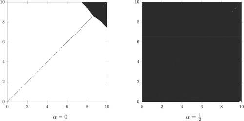
Figure 2. The candidates for an optimal strategy for $\alpha =0.3$ for different $x_{max}$ and N such that $\mathrm{\Delta }x=0.025$. In the white regions push-bottom is optimal and we use black for the regions where push-top is optimal. In the upper right corner numerical effects appear due to the imposed boundary conditions and the discretization. For increasing $x_{max}$, the region where these numerical effects happen move to the upper right corner. These effects do not influence the strategy in regions which are sufficiently far away.

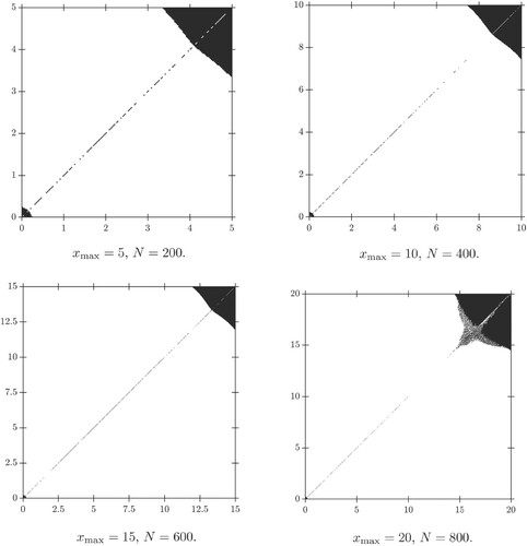
For $\alpha \in (0,\frac{1}{2}),$ we find that if the wealth of both companies is small (small depends on α), then the company with higher wealth should obtain the maximal drift rate (i.e. use push-top) whereas if the wealth process of at least one company is sufficiently large then the maximal drift rate 1 is assigned to the company with less wealth (i.e. use push-bottom). Hence, we can split our state space G into two regions, in one push-top is optimal and in the other push-bottom. Observe that the region where it is optimal to use push-top is increasing in α. This is due to the fact that if α increases the probability that exactly one firm survives is given more weight and the probability that none of the firms goes bankrupt has less influence.

Figures 3 and 4 show our candidates for the optimal strategy for different α. In the white regions push-bottom is optimal and we use black for the regions where push-top is optimal.

Figure 3. The candidates for an optimal strategy for $\alpha \in \{0.2,0.25,0.3,\frac{1}{3},0.35,0.4\}$ with $x_{max}=5$, N=400 and $w=\frac{3}{2}$. Here we only plot the strategies on $[0,1]\times [0,1]$ to focus on the black regions where push-top is chosen.

Figure 4. The candidates for an optimal strategy for $\alpha \in \{0.45,0.49,0.499,0.4999\}$ with $x_{max}=10$, N=800 and $w=\frac{3}{2}$. Here we only plot the strategies on the smaller set $[0,6]\times [0,6]$ to focus on the black regions where push-top is chosen.

Remark 4.2

Note that also McKean and Shepp in [20] obtain candidates for optimal strategies for $V^{\alpha }$. Since the description on how they obtain their results is a bit short, we provide a detailed explanation of our numerical method in the next section.

4.1. Numerical method: policy iteration and successive over-relaxation

Here we describe the numerical method we use to obtain the candidate for the optimal strategy. We combine two methods:

• policy iteration

• successive over-relaxation.

The idea of policy iteration used in reinforcement learning (cf. [5,23] for more details) is to start with an initial strategy (Step 0), compute the value of this strategy (Step 1) and improve the strategy appropriately (Step 2). Steps 1 and 2 are then repeated until a fixed point is found (or the value of the new strategy is very close to the value of the old strategy). In particular, a sequence of strategies with increasing values is constructed. For Step 1 observe that the value $J(x,y;u)$ of a given strategy $u=u(x,y)$ satisfies the linear partial differential equation (PDE) (18) $\begin{array}{r}\frac{1}{2}{J}_{xx}+\frac{1}{2}{J}_{yy}+u{J}_x+(1-u)J_y=0\text{on }G.\end{array}$(18) Note that the PDE for $V^{\alpha }$ given in (17(17) $\begin{array}{rl}\frac{1}{2}{V}_{xx}^{\alpha }+\frac{1}{2}{V}_{yy}^{\alpha }+\underset{u\in [0,1]}{sup}\{u{V}_x^{\alpha }+(1-u)V_y^{\alpha }\}& =\frac{1}{2}{V}_{xx}^{\alpha }+\frac{1}{2}{V}_{yy}^{\alpha }+max\{V_x^{\alpha },V_y^{\alpha }\}=0\text{on}G,\\ V^{\alpha }(x,0)& =\alpha (1-e^{-2x}),x\in [0,\mathrm{\infty }),\\ V^{\alpha }(0,y)& =\alpha (1-e^{-2y}),y\in [0,\mathrm{\infty }),\\ \underset{x,y\to \mathrm{\infty }}{lim}{V}^{\alpha }(x,y)& =1-\alpha .\end{array}$(17) ) is non-linear. To find J we restrict (18(18) $\begin{array}{r}\frac{1}{2}{J}_{xx}+\frac{1}{2}{J}_{yy}+u{J}_x+(1-u)J_y=0\text{on }G.\end{array}$(18) ) to a bounded state space and impose additional boundary conditions, discretize the new state space and the derivatives and solve the corresponding linear system of equations using successive over-relaxation, which is a variant of the Gauss–Seidel method and often has an improved convergence rate (see, e.g. [25, chapter 6]). For improving a strategy u in Step 2 we use the optimality criterion from the HJB equation (17(17) $\begin{array}{rl}\frac{1}{2}{V}_{xx}^{\alpha }+\frac{1}{2}{V}_{yy}^{\alpha }+\underset{u\in [0,1]}{sup}\{u{V}_x^{\alpha }+(1-u)V_y^{\alpha }\}& =\frac{1}{2}{V}_{xx}^{\alpha }+\frac{1}{2}{V}_{yy}^{\alpha }+max\{V_x^{\alpha },V_y^{\alpha }\}=0\text{on}G,\\ V^{\alpha }(x,0)& =\alpha (1-e^{-2x}),x\in [0,\mathrm{\infty }),\\ V^{\alpha }(0,y)& =\alpha (1-e^{-2y}),y\in [0,\mathrm{\infty }),\\ \underset{x,y\to \mathrm{\infty }}{lim}{V}^{\alpha }(x,y)& =1-\alpha .\end{array}$(17) ) and set $\begin{array}{r}{u}_{\text{new}}(x,y)={\text{𝟙}}_{\left\{J_x\right(x,y;u)\ge J_y(x,y;u\left)\right\}}.\end{array}$

Now we describe our method in more detail: we restrict ourselves to the bounded state space $S=[0,x_{max}]\times [0,y_{max}]$, where $x_{max}$ and $y_{max}$ are chosen sufficiently large. Due to the symmetry of our problem (16(16) $\begin{array}{r}{V}^{\alpha }(x,y)=\underset{u\in {\mathcal{U}}_{x,y}}{sup}(\alpha \mathbb{P}[{\mathrm{\Gamma }}^{x,y;u}=1]+(1-\alpha )\mathbb{P}[{\mathrm{\Gamma }}^{x,y;u}=2]).\end{array}$(16) ) we set $y_{max}=x_{max}$. We then obtain an approximation $V_S^{\alpha }$ for $V^{\alpha }$ on S as follows: for $(X_t^{x;u},Y_t^{y;u})\in (0,x_{max})\times (0,x_{max})$ divide a total drift of 1 among both companies in order to maximize the weighted probabilities in (16(16) $\begin{array}{r}{V}^{\alpha }(x,y)=\underset{u\in {\mathcal{U}}_{x,y}}{sup}(\alpha \mathbb{P}[{\mathrm{\Gamma }}^{x,y;u}=1]+(1-\alpha )\mathbb{P}[{\mathrm{\Gamma }}^{x,y;u}=2]).\end{array}$(16) ). If the wealth process of the first or second company exceeds $x_{max}$, then we consider this firm to survive forever and the other firm obtains a drift rate of 1. In particular, for $(x,y)\in S$ we set $\begin{array}{r}{V}_S^{\alpha }(x,x_{max})=\alpha e^{-2x}+(1-\alpha )(1-e^{-2x}),\\ V_S^{\alpha }(x_{max},y)=\alpha e^{-2y}+(1-\alpha )(1-e^{-2y}),\end{array}$where we use that the probability that a Brownian motion with unit drift starting in x hits zero equals $e^{-2x}$, see formula 1.2.4(1) in part II, chapter 2 in [6]. Moreover, let $\begin{array}{r}{V}_S^{\alpha }(x_{max},x_{max})=\alpha e^{-2x_{max}}+(1-\alpha )(1-e^{-2x_{max}}).\end{array}$Here we do not impose that $V(x_{max},x_{max})=1-\alpha$ to guarantee a boundary condition that is continuous in $(x_{max},x_{max})$. But observe that the boundary condition is not continuous in $(0,x_{max})$ and $(x_{max},0)$. Note that $V_S^{\alpha }\ge V^{\alpha }$ on S.

Step 0: To compute $V_S^{\alpha }$ we use policy iteration and thus, start with an initial guess $u_0$ for the optimal strategy for $V_S^{\alpha }$.

Step 1: The value $J(x,y;u_0)$ for this particular strategy satisfies (18(18) $\begin{array}{r}\frac{1}{2}{J}_{xx}+\frac{1}{2}{J}_{yy}+u{J}_x+(1-u)J_y=0\text{on }G.\end{array}$(18) ) on $(0,x_{max})\times (0,x_{max})$, where u is replaced by $u_0$. We discretize our state space S using an equidistant grid with $(N+1)\times (N+1)$ grid points and mesh size $\mathrm{\Delta }x=\frac{x_{max}}{N}$. For $i,j\in \{0,\dots ,N\}$ let $\begin{array}{rl}{\tilde{J}}_{i,j}& =J(i\mathrm{\Delta }x,j\mathrm{\Delta }x;u_0),\\ {\tilde{u}}_0(i,j)& =u_0(i\mathrm{\Delta }x,j\mathrm{\Delta }x).\end{array}$Then we have the following boundary conditions for $\tilde{J}$: $\begin{array}{rlrl}{\tilde{J}}_{0,j}& =\alpha (1-e^{-2j\mathrm{\Delta }x}),& & j=0,\dots ,N-1,\\ {\tilde{J}}_{i,0}& =\alpha (1-e^{-2i\mathrm{\Delta }x}),& & i=0,\dots ,N-1,\\ {\tilde{J}}_{N,j}& =\alpha e^{-2j\mathrm{\Delta }x}+(1-\alpha )(1-e^{-2j\mathrm{\Delta }x}),& & j=0,\dots ,N,\\ {\tilde{J}}_{i,N}& =\alpha e^{-2i\mathrm{\Delta }x}+(1-\alpha )(1-e^{-2i\mathrm{\Delta }x}),& & i=0,\dots ,N.\end{array}$Using central finite difference quotients for (18(18) $\begin{array}{r}\frac{1}{2}{J}_{xx}+\frac{1}{2}{J}_{yy}+u{J}_x+(1-u)J_y=0\text{on }G.\end{array}$(18) ) we observe that our approximation $\tilde{J}$ satisfies $\begin{array}{r}{\tilde{J}}_{i,j}=c_1{\tilde{J}}_{i+1,j}+c_2{\tilde{J}}_{i-1,j}+c_3{\tilde{J}}_{i,j+1}+c_4{\tilde{J}}_{i,j-1}\end{array}$for $i,j=1,\dots ,N-1$, where $\begin{array}{rlrl}{c}_1& =\frac{1}{4}[1+\mathrm{\Delta }x{\tilde{u}}_0(i,j\left)\right],& & c_2=\frac{1}{4}[1-\mathrm{\Delta }x{\tilde{u}}_0(i,j\left)\right],\\ c_3& =\frac{1}{4}[1+\mathrm{\Delta }x(1-{\tilde{u}}_0(i,j\left))\right],& & c_4=\frac{1}{4}[1-\mathrm{\Delta }x(1-{\tilde{u}}_0(i,j\left))\right].\end{array}$To solve this system of $(N-1{)}^2$ linear equations, we use successive over-relaxation (SOR): we start with an initial guess $J_{i,j}^{\left(0\right)}$, $i,j=1,\dots ,N-1$, and define iteratively $\begin{array}{r}{J}_{i,j}^{(k+1)}=(1-w)J_{i,j}^{\left(k\right)}+w\{c_1{J}_{i+1,j}^{\left(k\right)}+c_2{J}_{i-1,j}^{(k+1)}+c_3{J}_{i,j+1}^{\left(k\right)}+c_4{J}_{i,j-1}^{(k+1)}\}\end{array}$for $i,j=1,\dots ,N-1$ and $k\in \mathbb{N}$, where $w\in (0,2)$ is the so-called relaxation parameter, see, e.g. [25] for a detailed analysis of the SOR method and [15,17,18] for an overview. For w=1 one obtains the Gauss–Seidel method. We continue until $\Vert J^{(k+1)}-J^{\left(k\right)}{\Vert }_{\mathrm{\infty }}\le ϵ$ for a given approximation error $ϵ>0$ and then set $\tilde{J}=J^{(k+1)}$. This is our approximation for the value $J(.,.;u_0)$ of the strategy $u_0$ on the grid $\left\{\right(i\mathrm{\Delta }x,j\mathrm{\Delta }x){\}}_{i,j=0,\dots ,N}$.

Step 2: To improve the strategy $u_0$, we use the discretized optimality condition from the HJB equation (17(17) $\begin{array}{rl}\frac{1}{2}{V}_{xx}^{\alpha }+\frac{1}{2}{V}_{yy}^{\alpha }+\underset{u\in [0,1]}{sup}\{u{V}_x^{\alpha }+(1-u)V_y^{\alpha }\}& =\frac{1}{2}{V}_{xx}^{\alpha }+\frac{1}{2}{V}_{yy}^{\alpha }+max\{V_x^{\alpha },V_y^{\alpha }\}=0\text{on}G,\\ V^{\alpha }(x,0)& =\alpha (1-e^{-2x}),x\in [0,\mathrm{\infty }),\\ V^{\alpha }(0,y)& =\alpha (1-e^{-2y}),y\in [0,\mathrm{\infty }),\\ \underset{x,y\to \mathrm{\infty }}{lim}{V}^{\alpha }(x,y)& =1-\alpha .\end{array}$(17) ) for $V^{\alpha }$. More precisely, for $i,j=1,\dots ,N-1$ define $\begin{array}{r}{\tilde{u}}_{\text{new}}(i,j)=\{\begin{array}{lc}1,& {\tilde{J}}_{i+1,j}-{\tilde{J}}_{i-1,j}\ge {\tilde{J}}_{i,j+1}-{\tilde{J}}_{i,j-1},\\ 0,& \text{else}\end{array}\end{array}$and for the grid points on the boundary we use forward or backward difference quotients and set ${\tilde{u}}_{\text{new}}(i,j)=1$ if

with $i,j=1,\dots ,N-1$. Otherwise we set ${\tilde{u}}_{\text{new}}(i,j)=0.$ For $i,j=0,\dots ,N$ define $\begin{array}{r}{u}_{\text{new}}(i\mathrm{\Delta }x,j\mathrm{\Delta }x)={\tilde{u}}_{\text{new}}(i,j).\end{array}$We then continue with Steps 1 and 2 for the new strategy $u_{\text{new}}$ and proceed until we obtain a policy $u_{\ell +1}$ with $\Vert J(.,.;u_{\ell +1})-J(.,.;u_{\ell }){\Vert }_{\mathrm{\infty }}\le \delta$ for a given approximation error $\delta >0$. Finally, our approximation for $V_S^{\alpha }$ is given by $J(.,.;u_{\ell +1})$ and $u_{\ell +1}$ is a candidate for the optimal strategy for $V^{\alpha }$.

Observe that we only construct a candidate for the optimal strategy on the grid $\begin{array}{r}\{(i\mathrm{\Delta }x,j\mathrm{\Delta }x){\}}_{i,j=0,\dots ,N}.\end{array}$

Remark 4.3

1. For every strategy $u_{\ell }$ in the policy iteration procedure we have to compute its value and therefore, use successive over-relaxation for any of these strategies separately.

2. For deriving the value of the initial strategy $u_0$ we choose $J_{i,j}^{\left(0\right)}=0$ for all $i,j=1,\dots ,N-1$ as initialization for the successive over-relaxation. For every updated strategy $u_{\ell }$ afterwards we use the approximation for the value $J(.,.;u_{\ell -1})$ of the old strategy $u_{\ell -1}$ as initial guess.

3. In our setting, different relaxation parameters w yield the same candidate for the optimal strategy (except for some differences on the set $\{x=y\}$ which is not surprising because both companies can be pushed on this set). Nevertheless, the speed of convergence heavily depends on w.

Acknowledgments

We thank two anonymous referees for carefully reading the manuscript and highly appreciate their comments, which contributed to improve our paper.

Disclosure statement

No potential conflict of interest was reported by the authors.

Additional information

Funding

Both authors gratefully acknowledge the partial support by the Austrian Science Fund (Fonds zur Förderung der wissenschaftlichen Forschung) under grant P30864-N35.

Appendix

In this appendix, we prove auxiliary statements for the results in Section 3. The following results describe the behaviour of V and its derivatives for large x or y. Their proofs are based on the proofs of Lemma 4.2, Lemma 6.1 and Lemma 6.2 in [13]. Since in our setting the proofs use similar ideas but are shorter we present them in detail.

Lemma A.1

It holds that $\begin{array}{rl}& \underset{y\to \mathrm{\infty }}{lim}V(x,y)=1,\text{uniformly in }x\ge 0,\\ & \underset{x\to \mathrm{\infty }}{lim}V(x,y)=1,\text{uniformly in }y\ge 0.\end{array}$

Proof.

Due to the symmetry of the value function V we only show the first claim. Let $x\ge 0$ and y>0. Using the strategy $\tilde{u}$ with ${\tilde{u}}^{\left(1\right)}\equiv 0$ we obtain a lower bound for V . More precisely, $\begin{array}{r}V(x,y)\ge J(x,y;\tilde{u})=1-e^{-2y},\end{array}$

because the first company is ruined almost surely and the survival probability of a Brownian motion with unit drift starting in y>0 equals $1-e^{-2y}$. Since $V\le 1$, the claim follows.

Lemma A.2

One has $\begin{array}{r}\underset{x\to \mathrm{\infty }}{lim}{V}_x(x,y)=0\text{and}\underset{x\to \mathrm{\infty }}{lim}{V}_y(x,y)=0\end{array}$for y>0 and uniformly for $y\ge \underset{\_}{y}$ for all $\underset{\_}{y}>0$. In addition, $\begin{array}{r}\underset{y\to \mathrm{\infty }}{lim}{V}_x(x,y)=0\text{and}\underset{y\to \mathrm{\infty }}{lim}{V}_y(x,y)=0\end{array}$for x>0 and uniformly for $x\ge \underset{\_}{x}$ for all $\underset{\_}{x}>0$.

Proof.

Let $\tilde{V}(x,y)=V(x,y)-1$. Then by Lemma A.1 it follows that $\underset{(x,y)\to \mathrm{\infty }}{lim}\tilde{V}(x,y)=0$. Let $(x_0,y_0)\in G$ and denote by $B=B(x_0,y_0;\frac{1}{2}\wedge x_0\wedge y_0)$ the open ball around $(x_0,y_0)$ with radius $r_0:=\frac{1}{2}\wedge x_0\wedge y_0$. Let $ϵ>0$. For $\Vert (x_0,y_0)\Vert =\sqrt{x_0^2+y_0^2}$ sufficiently large it holds that (A1) $\begin{array}{r}\underset{(x,y)\in B}{sup}|\tilde{V}(x,y)|\le ϵ.\end{array}$(A1) Observe that $\tilde{V}$ satisfies $\begin{array}{r}F(x,y,\tilde{V},D\tilde{V},D^2\tilde{V}):=\frac{1}{2}{\tilde{V}}_{xx}+\frac{1}{2}{\tilde{V}}_{yy}+max\{{\tilde{V}}_x,{\tilde{V}}_y\}=0.\end{array}$We now restrict $\tilde{V}$ to B. To apply Theorem 3.1 in [22] note that one can easily check that Conditions (F0), (F1), (F3), (F4), and the first part of (F2) are fulfilled. It remains to show the Lipschitz property of F in $(\tilde{V},D\tilde{V})$. For this purpose observe that $\begin{array}{r}|F(x,y,\tilde{V},D\tilde{V},D^2\tilde{V})-F(x,y,U,DU,D^2\tilde{V})|=|max\{{\tilde{V}}_x,{\tilde{V}}_y\}-max\{U_x,U_y\}|.\end{array}$Now we distinguish several cases:

For $\boxed{{\displaystyle {\tilde{V}}_x\ge {\tilde{V}}_y,U_x\ge U_y}}$ we have $\begin{array}{r}|max\{{\tilde{V}}_x,{\tilde{V}}_y\}-max\{U_x,U_y\left\}\right|=|{\tilde{V}}_x-U_x|.\end{array}$If $\boxed{{\displaystyle {\tilde{V}}_x\ge {\tilde{V}}_y,U_x\le U_y}}$ it holds that $\begin{array}{rl}|max\{{\tilde{V}}_x,{\tilde{V}}_y\}-max\{U_x,U_y\left\}\right|& =|{\tilde{V}}_x-U_y|\le |{\tilde{V}}_x-U_x|+|U_x-U_y|=|{\tilde{V}}_x-U_x|+U_y-U_x\\ & \le 2|{\tilde{V}}_x-U_x|+|{\tilde{V}}_y-U_y|+{\tilde{V}}_y-{\tilde{V}}_x\\ & \le 2|{\tilde{V}}_x-U_x|+|{\tilde{V}}_y-U_y|.\end{array}$The cases $\boxed{{\displaystyle {\tilde{V}}_x\le {\tilde{V}}_y,U_x\le U_y}}$ and $\boxed{{\displaystyle {\tilde{V}}_x\le {\tilde{V}}_y,U_x\ge U_y}}$ can be treated similarly. Hence, $\begin{array}{r}|F(x,y,\tilde{V},D\tilde{V},D^2\tilde{V})-F(x,y,U,DU,D^2\tilde{V})|\le 2|{\tilde{V}}_x-U_x|+|{\tilde{V}}_y-U_y|\end{array}$and therefore, Condition (F2) is fulfilled for K=2.

Theorem 3.1 in [22] now implies that for all $\alpha \in (0,\overline{\alpha })$ for some $\overline{\alpha }\in (0,1)$ it holds that $\begin{array}{r}\Vert \tilde{V}{\Vert }_{2,\alpha ;B}^{\left(0\right)}\le Cϵ,\end{array}$where ε is an upper bound for $|\tilde{V}|$ on B, see (A1(A1) $\begin{array}{r}\underset{(x,y)\in B}{sup}|\tilde{V}(x,y)|\le ϵ.\end{array}$(A1) ), and $C=C\left(\alpha \right)>0$. For the definition of $\Vert .{\Vert }_{2,\alpha ;B}^{\left(0\right)}$ see Section 2 in [22]. In particular, this implies (A2) $\begin{array}{rl}\underset{(x,y)\in B(x_0,y_0;\frac{r_0}{2})}{sup}|{\tilde{V}}_x(x,y)|& \le \frac{2}{r_0}Cϵ,\\ \underset{(x,y)\in B(x_0,y_0;\frac{r_0}{2})}{sup}|{\tilde{V}}_y(x,y)|& \le \frac{2}{r_0}Cϵ.\end{array}$(A2) With $V_x={\tilde{V}}_x$ and $V_y={\tilde{V}}_y$ the claim follows.

Note that we cannot conclude that the convergence is uniformly in $x_0$ or $y_0$ because the right-hand side of (A2(A2) $\begin{array}{rl}\underset{(x,y)\in B(x_0,y_0;\frac{r_0}{2})}{sup}|{\tilde{V}}_x(x,y)|& \le \frac{2}{r_0}Cϵ,\\ \underset{(x,y)\in B(x_0,y_0;\frac{r_0}{2})}{sup}|{\tilde{V}}_y(x,y)|& \le \frac{2}{r_0}Cϵ.\end{array}$(A2) ) explodes e.g. for $x_0\to 0$ and $y_0$ sufficiently large.

Lemma A.3

If either

• $\underset{n\to \mathrm{\infty }}{lim}{x}_n=\mathrm{\infty }$ and $\underset{n\to \mathrm{\infty }}{lim}{y}_n=0$ or

• $\underset{n\to \mathrm{\infty }}{lim}{y}_n=\mathrm{\infty }$ and $\underset{n\to \mathrm{\infty }}{lim}{x}_n=0$

then $\begin{array}{r}\underset{n\to \mathrm{\infty }}{lim}D(x_n,y_n)=0.\end{array}$

Proof.

Due to the symmetry of the value function V we only consider the case where $\underset{n\to \mathrm{\infty }}{lim}{x}_n$ $=\mathrm{\infty }$ and $\underset{n\to \mathrm{\infty }}{lim}{y}_n=0$. Moreover, we only show $\begin{array}{r}\underset{n\to \mathrm{\infty }}{lim}{V}_x(x_n,y_n)=0\end{array}$because similar arguments can be used for deriving $\underset{n\to \mathrm{\infty }}{lim}{V}_y(x_n,y_n)=0$.

Let $\delta ,K>0$ and $N\in \mathbb{N}$ such that $x_n\ge K$ and $y_n\le \delta$ for all $n\ge N$. Now let $x\ge K$ and $y\in (0,\delta ]$. Let $ϵ\in (0,\frac{x}{2})$. As in the proof of Lemma 4.2 in [13] let $u^{\ast }$ be a strategy that is optimal in (3(3) $\begin{array}{r}V(x,y)=\underset{u\in {\mathcal{U}}_{x,y}}{sup}J(x,y;u).\end{array}$(3) ) for starting in $(x,y)$; in particular $u_s^{\ast }={\hat{u}}^{\ast }(X_s^{x;u^{\ast }},Y_s^{y;u^{\ast }}),s\in [0,\mathrm{\infty }),$ for some Borel measurable ${\hat{u}}^{\ast }$. If no optimal strategy exists we use an η – optimal strategy for $\eta >0$ and proceed similarly. We now define a strategy $\tilde{u}$ for the process started in $(x-ϵ,y)$ in such a way that the paths of the two processes $(X^{x;u^{\ast }},Y^{y;u^{\ast }})$ and $(X^{x-ϵ;\tilde{u}},Y^{y;\tilde{u}})$ move parallel having distance ε in the first component. For this purpose let $\begin{array}{r}{\tilde{u}}_s={\hat{u}}^{\ast }(X_s^{x;u^{\ast }},Y_s^{y;u^{\ast }})={\hat{u}}^{\ast }(X_s^{x-ϵ;\tilde{u}}+ϵ,Y_s^{y;\tilde{u}}).\end{array}$Observe that using $\tilde{u}$ the process started in $(x-ϵ,y)$ is ruined not later than the optimally controlled process started in $(x,y)$ and can be ruined earlier with positive probability. Hence, we modify $\tilde{u}$ after the first ruin time $\tau (x-ϵ,y;\tilde{u})$ in such a way that it becomes admissible, i.e. $\tilde{u}\in {\mathcal{U}}_{x-ϵ,y}$, which means that after the first ruin time the surviving process obtains the maximal drift rate until it hits zero. If both processes are ruined, then ${\tilde{u}}_s$ is set to $(0,0)$ afterwards.

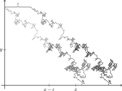
To sum up, by the definition of strategy $\tilde{u}$ it holds that $\begin{array}{r}(X_s^{x;\tilde{u}},Y_s^{y;\tilde{u}})=(X_s^{x;u^{\ast }}-ϵ,Y_s^{y;u^{\ast }})\text{on}[0,\tau (x-ϵ,y;\tilde{u})].\end{array}$Figure A1 depicts two different trajectories for our controlled process started in $(x,y)$ and the corresponding shifted trajectories for the process started in $(x-ϵ,y)$ until one firm is ruined when started in $(x-ϵ,y)$.

Figure A1. Two different trajectories for the controlled process started in $(x,y)$ and the corresponding shifted trajectories for the process started in $(x-ϵ,y)$ until one firm is ruined when started in $(x-ϵ,y)$, see the proof of Lemma A.3.

Now let $\tau =\tau (x-ϵ,y;\tilde{u})$ be the first time at which one company is ruined if the initial endowment is given by $(x-ϵ,y)$ and strategy $\tilde{u}$ is used. Then $V(x-ϵ,y)\ge J(x-ϵ,y;\tilde{u})$ and the optimality of $u^{\ast }$ for $V(x,y)$ yield (A3) $\begin{array}{rl}V(x,y)-V(x-ϵ,y)& \le \mathbb{P}[\tau <\mathrm{\infty },X_{\tau }^{x-ϵ;\tilde{u}}=0]\int [V(ϵ,z)-V(0,z)]\mathrm{d}{F}^{ϵ}\left(z\right)\\ & +\mathbb{P}[\tau <\mathrm{\infty },Y_{\tau }^{y;\tilde{u}}=0]\int \mathbb{P}[\underset{t\in [0,\mathrm{\infty })}{inf}\{B_t+t\}\in (-z,-z+ϵ\left]\right]\mathrm{d}{G}^{ϵ}\left(z\right),\end{array}$(A3) where $\text{d}{F}^{ϵ}$ denotes the conditional distribution of $Y_{\tau }^{y;\tilde{u}}=Y_{\tau }^{y;u^{\ast }}$ given $\{\tau <\mathrm{\infty },X_{\tau }^{x-ϵ;\tilde{u}}=0\}$ and $\text{d}{G}^{ϵ}$ denotes the conditional distribution of $X_{\tau }^{x;u^{\ast }}$ conditioned on $\{\tau <\mathrm{\infty },Y_{\tau }^{y;\tilde{u}}=0\}$.

From Lemma 3.5, we know that $V_x(0,z)<V_y(0,z)=2e^{-2z}$ for all z>0 and hence, $\begin{array}{r}\underset{ϵ\downarrow 0}{lim}\frac{V(ϵ,z)-V(0,z)}{ϵ}=V_x(0,z)\in [0,2e^{-2z}].\end{array}$ In particular, $V(ϵ,z)-V(0,z)\le 4ϵ$ for all $ϵ>0$ sufficiently small. Moreover, it holds that $\begin{array}{r}\mathbb{P}[\tau <\mathrm{\infty },X_{\tau }^{x-ϵ;\tilde{u}}=0]\le \mathbb{P}[{\tau }_1<{\tau }_2],\end{array}$where $\begin{array}{rl}{\tau }_1& =inf\{t\in [0,\mathrm{\infty }):\frac{x}{2}+B_t=0\},\\ {\tau }_2& =inf\{t\in [0,\mathrm{\infty }):\delta +t+{\hat{B}}_t=0\}.\end{array}$Using formula 1.2.4(1) in part II, chapter 2 in [6] for the second summand on the right-hand side of (A3(A3) $\begin{array}{rl}V(x,y)-V(x-ϵ,y)& \le \mathbb{P}[\tau <\mathrm{\infty },X_{\tau }^{x-ϵ;\tilde{u}}=0]\int [V(ϵ,z)-V(0,z)]\mathrm{d}{F}^{ϵ}\left(z\right)\\ & +\mathbb{P}[\tau <\mathrm{\infty },Y_{\tau }^{y;\tilde{u}}=0]\int \mathbb{P}[\underset{t\in [0,\mathrm{\infty })}{inf}\{B_t+t\}\in (-z,-z+ϵ\left]\right]\mathrm{d}{G}^{ϵ}\left(z\right),\end{array}$(A3) ) yields $\begin{array}{rl}& \mathbb{P}[\tau <\mathrm{\infty },Y_{\tau }^{y;\tilde{u}}=0]\int \mathbb{P}[\underset{t\in [0,\mathrm{\infty })}{inf}\{B_t+t\}\in (-z,-z+ϵ\left]\right]\mathrm{d}{G}^{ϵ}\left(z\right)\\ & =\mathbb{P}[\tau <\mathrm{\infty },Y_{\tau }^{y;\tilde{u}}=0](e^{2ϵ}-1)\int e^{-2z}\mathrm{d}{G}^{ϵ}\left(z\right)\\ & \le \mathbb{P}[\tau <\mathrm{\infty },Y_{\tau }^{y;\tilde{u}}=0](e^{2ϵ}-1)(e^{-x}+\mathbb{P}[X_{\tau }^{x;u^{\ast }}<\frac{x}{2}|\tau <\mathrm{\infty },Y_{\tau }^{y;\tilde{u}}=0])\\ & \le (e^{2ϵ}-1)(e^{-x}+\mathbb{P}[X_{\tau }^{x;u^{\ast }}<\frac{x}{2},\tau <\mathrm{\infty },Y_{\tau }^{y;\tilde{u}}=0])\\ & \le (e^{2ϵ}-1)(e^{-x}+\mathbb{P}[{\tau }_1<{\tau }_2]).\end{array}$To sum up, we have (A4) $\begin{array}{rl}0\le V_x(x,y)& =\underset{ϵ\downarrow 0}{lim}\frac{V(x,y)-V(x-ϵ,y)}{ϵ}\le \underset{ϵ\downarrow 0}{lim}\{4\mathbb{P}[{\tau }_1<{\tau }_2]+\frac{e^{2ϵ}-1}{ϵ}(e^{-x}+\mathbb{P}[{\tau }_1<{\tau }_2])\}\\ & \le 6\mathbb{P}[{\tau }_1<{\tau }_2]+2e^{-x}.\end{array}$(A4) Since $\mathbb{P}[{\tau }_1<{\tau }_2]\to 0$ as $\delta \downarrow 0$ uniformly in $x\ge K$ we conclude that $\begin{array}{r}\underset{n\to \mathrm{\infty }}{lim}{V}_x(x_n,y_n)=0.\end{array}$

References

- S. Ankirchner, R. Hesse, and M. Klein, On the joint survival probability of two collaborating firms, J. Appl. Probab. (2023), pp. 1–16.
- F. Avram, Z. Palmowski, and M. Pistorius, A two-dimensional ruin problem on the positive quadrant, Insurance Math. Econom. 42(1) (2008), pp. 227–234.
- F. Avram, Z. Palmowski, and M. Pistorius, Exit problem of a two-dimensional risk process from the quadrant: exact and asymptotic results, Ann. Appl. Probab. 18(6) (2008), pp. 2421–2449.
- V.E. Beneš, Full “bang” to reduce predicted miss is optimal, SIAM J. Control Optim. 14(1) (1976), pp. 62–84.
- D.P. Bertsekas, Reinforcement Learning and Optimal Control, Athena Scientific Optimization and Computation Series, Athena Scientific, 2019.
- A.N. Borodin and P. Salminen, Handbook of Brownian Motion – Facts and Formulae, 2nd ed., Probability and its Applications, Birkhäuser Verlag, Basel, 2002.
- W.-S. Chan, H. Yang, and L. Zhang, Some results on ruin probabilities in a two-dimensional risk model, Insurance Math. Econom. 32(3) (2003), pp. 345–358.
- J.F. Collamore, Hitting probabilities and large deviations, Ann. Probab. 24(4) (1996), pp. 2065–2078.
- P. Grandits, A ruin problem for a two-dimensional Brownian motion with controllable drift in the positive quadrant, Teor. Veroyatn. Primen. 64(4) (2019), pp. 811–823.
- P. Grandits, A two-dimensional dividend problem for collaborating companies and an optimal stopping problem, Scand. Actuar. J. 2019(1) (2019), pp. 80–96.
- P. Grandits, On the gain of collaboration in a two dimensional ruin problem, Eur. Actuar. J. 9(2) (2019), pp. 635–644.
- P. Grandits, A singular perturbed ruin problem for a two dimensional Brownian motion in the positive quadrant. https://fam.tuwien.ac.at/~pgrand/sing_pert.pdf, preprint, 2020.
- P. Grandits, Some global topological properties of a free boundary problem appearing in a two dimensional controlled ruin problem, Math. Control Signals Syst. 35 (2023), pp. 927–949.
- P. Grandits and M. Klein, Ruin probability in a two-dimensional model with correlated Brownian motions, Scand. Actuar. J. 2021(5) (2021), pp. 362–379.
- A. Greenbaum, Iterative Methods for Solving Linear Systems, Frontiers in Applied Mathematics; Vol. 17, Society for Industrial and Applied Mathematics (SIAM), Philadelphia, PA, 1997.
- J.-W. Gu, M. Steffensen, and H. Zheng, Optimal dividend strategies of two collaborating businesses in the diffusion approximation model, Math. Oper. Res. 43(2) (2018), pp. 377–398.
- W. Hackbusch, Iterative Solution of Large Sparse Systems of Equations, 2nd ed., Applied Mathematical Sciences; Vol. 95, Springer, 2016.
- A. Iserles, A First Course in the Numerical Analysis of Differential Equations, Cambridge Texts in Applied Mathematics, Cambridge University Press, Cambridge, 1996.
- N. Kulenko and H. Schmidli, Optimal dividend strategies in a Cramér-Lundberg model with capital injections, Insurance Math. Econom. 43(2) (2008), pp. 270–278.
- H.P. McKean and L.A. Shepp, The advantage of capitalism vs. socialism depends on the criterion, J. Math. Sci. 139(3) (2006), pp. 6589–6594.
- J.R. Munkres, Topology, Prentice Hall, Inc., Upper Saddle River, NJ, 2000.
- M. Safonov, On the boundary value problems for fully nonlinear elliptic equations of second order. Math. Res. Report No. MMR 049-94, Austral. Nat. Univ., Canberra, 1994.
- R.S. Sutton and A.G. Barto, Reinforcement Learning: An Introduction, 2nd ed., Adaptive Computation and Machine Learning, MIT Press, Cambridge, MA, 2018.
- A.Y. Veretennikov, On the criteria for existence of a strong solution of a stochastic equation, Theory Probab. Appl. 27(3) (1983), pp. 441–449.
- D.M. Young, Iterative Solution of Large Linear Systems, Academic Press, New York-London, 1971.