Discounted nonzero-sum optimal stopping games under Poisson random intervention times

Abstract

We present solutions to some discounted nonzero-sum optimal stopping games of two players related to the perpetual game-type contingent claims with payoffs representing linear functions of the running values of a geometric Brownian motion. It is assumed that the underlying process can be stopped by the both players only at certain random intervention times which coincide with the jump times of the two appropriate independent Poisson processes. The optimal stopping times forming a Nash equilibrium are shown to be the first times at which the underlying process is either below or above certain lower or upper constant boundaries at the jump times of the appropriate Poisson processes. The proof is based on the reductions of the original games to the associated coupled free-boundary problems and the solutions to the latter problems by means of the smooth-fit conditions at the optimal boundaries for every player. We show that the optimal stopping constant lower and upper boundaries are determined as (possibly multiple) solutions to the equivalent coupled systems of arithmetic equations. The obtained results can be interpreted as the rational valuation of some perpetual randomized Bermudian game-type contingent claims in the Black-Merton-Scholes model.

Keywords:

• Nonzero-sum optimal stopping game
• Brownian motion
• Poisson process
• random intervention times
• free-boundary problem
• instantaneous stopping and smooth fit
• perpetual randomized Bermudian contingent claims
• a local time-space formula

2020 Mathematics Subject Classifications:

• Primary 60G40
• 34K10
• 91G20
• Secondary 60J60
• 34L30
• 91B25

1. Introduction

The main aim of this paper is to present solutions to the discounted nonzero-sum optimal stopping game formulated in (3(3) $\begin{array}{r}{J}_1(\tau ,\zeta )=E[{\int }_0^{\tau \wedge \zeta }{e}^{-\mathrm{rs}}{X}_s\mathrm{d}s+e^{-\mathrm{r\tau }}\frac{L_1}{r}I(\tau \le \zeta )+e^{-\mathrm{r\zeta }}\frac{K_1}{r}I(\zeta <\tau )]\end{array}$(3) )–(5(5) $\begin{array}{r}{J}_1(\tau ,{\zeta }_{\ast })\le J_1({\tau }_{\ast },{\zeta }_{\ast })\mathrm{and}{J}_2({\zeta }_{\ast },{\tau }_{\ast })\le J_2(\zeta ,{\tau }_{\ast })\end{array}$(5) ) for the geometric Brownian motion $X=(X_t{)}_{t\ge 0}$ defined in (1(1) $\begin{array}{r}{X}_t=\mathrm{xexp}((r-\delta -{\sigma }^2/2)t+\sigma B_t)\end{array}$(1) ) and (2(2) $\begin{array}{r}\mathrm{d}{X}_t=(r-\delta )X_t\mathrm{d}t+\sigma X_t\mathrm{d}{B}_t(X_0=x)\end{array}$(2) ) observed by the two players at the jump times of two independent Poisson processes. Here, for a precise formulation of the problem, let us consider a probability space $(\mathrm{\Omega },\mathcal{F},P)$ with a standard Brownian motion $B=(B_t{)}_{t\ge 0}$. We assume that the process $X=(X_t{)}_{t\ge 0}$ is a geometric Brownian motion defined by: (1) $\begin{array}{r}{X}_t=\mathrm{xexp}((r-\delta -{\sigma }^2/2)t+\sigma B_t)\end{array}$(1) which solves the stochastic differential equation: (2) $\begin{array}{r}\mathrm{d}{X}_t=(r-\delta )X_t\mathrm{d}t+\sigma X_t\mathrm{d}{B}_t(X_0=x)\end{array}$(2) where r>0, $\delta >0$, and $\sigma >0$ are given constants, and x>0 is fixed. Suppose that there exist Poisson processes $N^i=(N_t^i{)}_{t\ge 0}$, for i = 1, 2, such that $N^1$ has the intensity $\lambda >0$ and $N^2$ has the intensity $\varkappa >0$, which are independent of each other as well as of the driving standard Brownian motion B. Denote by $({\tau }_l{)}_{l\in \mathbb{N}}$ and $({\zeta }_k{)}_{k\in \mathbb{N}}$ the sets of jump times of the processes $N^i$, for i = 1, 2, so that the differences ${\tau }_1,{\tau }_2-{\tau }_1,\dots ,{\tau }_l-{\tau }_{l-1},\dots$ and ${\zeta }_1,{\zeta }_2-{\zeta }_1,\dots ,{\zeta }_k-{\zeta }_{k-1},\dots$, for $l,k\in \mathbb{N}$, are independent exponential random variables with the means $1/\lambda$ and $1/\varkappa$, respectively. We now define the filtrations $({\mathcal{G}}_{{\tau }_l}{)}_{l\in \mathbb{N}}$ and $({\mathcal{H}}_{{\zeta }_k}{)}_{k\in \mathbb{N}}$ as ${\mathcal{G}}_{{\tau }_l}=\sigma (X_{{\tau }_1},\dots ,X_{{\tau }_l})$ and ${\mathcal{H}}_{{\zeta }_k}=\sigma (X_{{\zeta }_1},\dots ,X_{{\zeta }_k})$, for each $l,k\in \mathbb{N}$, and denote by $T(\lambda )$ and $Z(\varkappa )$ the sets of stopping times with respect to the filtrations $({\mathcal{G}}_{{\tau }_l}{)}_{l\in \mathbb{N}}$ and $({\mathcal{H}}_{{\zeta }_k}{)}_{k\in \mathbb{N}}$, respectively.

Assume that the process X represents the price of a risky asset in a financial market, while the supremum and infimum in (8(8) $\begin{array}{r}{V}_{\ast }(x)=\underset{\tau \in T(\lambda )}{sup}{E}_x[e^{-\mathrm{r\tau }}(\frac{L_1}{r}-\frac{X_{\tau }}{\delta })I(\tau \le {\zeta }_{\ast })+e^{-r{\zeta }_{\ast }}(\frac{K_1}{r}-\frac{X_{{\zeta }_{\ast }}}{\delta })I({\zeta }_{\ast }<\tau )]\end{array}$(8) ) and (9(9) $\begin{array}{r}{U}_{\ast }(x)=\underset{\zeta \in Z(\varkappa )}{inf}{E}_x[e^{-\mathrm{r\zeta }}(\frac{K_2}{r}-\frac{X_{\zeta }}{\delta })I(\zeta \le {\tau }_{\ast })+e^{-r{\tau }_{\ast }}(\frac{L_2}{r}-\frac{X_{{\tau }_{\ast }}}{\delta })I({\tau }_{\ast }<\zeta )]\end{array}$(9) ) as in the equivalent reformulation of the nonzero-sum optimal stopping game of (3(3) $\begin{array}{r}{J}_1(\tau ,\zeta )=E[{\int }_0^{\tau \wedge \zeta }{e}^{-\mathrm{rs}}{X}_s\mathrm{d}s+e^{-\mathrm{r\tau }}\frac{L_1}{r}I(\tau \le \zeta )+e^{-\mathrm{r\zeta }}\frac{K_1}{r}I(\zeta <\tau )]\end{array}$(3) )–(5(5) $\begin{array}{r}{J}_1(\tau ,{\zeta }_{\ast })\le J_1({\tau }_{\ast },{\zeta }_{\ast })\mathrm{and}{J}_2({\zeta }_{\ast },{\tau }_{\ast })\le J_2(\zeta ,{\tau }_{\ast })\end{array}$(5) ) are taken over all stopping times τ and ζ from the sets $T(\lambda )$ and $Z(\varkappa )$, as well as the expectations there are taken with respect to the (unique) risk-neutral (or martingale) probability measure P. In this case, it follows from the natural extensions of the results of [30,33] that the values $V_{\ast }(x)$ and $U_{\ast }(x)$ from (8(8) $\begin{array}{r}{V}_{\ast }(x)=\underset{\tau \in T(\lambda )}{sup}{E}_x[e^{-\mathrm{r\tau }}(\frac{L_1}{r}-\frac{X_{\tau }}{\delta })I(\tau \le {\zeta }_{\ast })+e^{-r{\zeta }_{\ast }}(\frac{K_1}{r}-\frac{X_{{\zeta }_{\ast }}}{\delta })I({\zeta }_{\ast }<\tau )]\end{array}$(8) ) and (9(9) $\begin{array}{r}{U}_{\ast }(x)=\underset{\zeta \in Z(\varkappa )}{inf}{E}_x[e^{-\mathrm{r\zeta }}(\frac{K_2}{r}-\frac{X_{\zeta }}{\delta })I(\zeta \le {\tau }_{\ast })+e^{-r{\tau }_{\ast }}(\frac{L_2}{r}-\frac{X_{{\tau }_{\ast }}}{\delta })I({\tau }_{\ast }<\zeta )]\end{array}$(9) ) can be interpreted as the rational (or no-arbitrage) prices of a (randomised Bermudian) game-type contingent claim described below with the strikes $0<L_i<K_j$, for every i, j = 1, 2, in the Black-Merton-Scholes model, respectively. Note that, when $L_1=L_2$ and $K_1=K_2$ holds, the original nonzero-sum optimal stopping game degenerates into a zero-sum one, so that the equality $V_{\ast }(x)=U_{\ast }(x)$ holds for the value functions in (8(8) $\begin{array}{r}{V}_{\ast }(x)=\underset{\tau \in T(\lambda )}{sup}{E}_x[e^{-\mathrm{r\tau }}(\frac{L_1}{r}-\frac{X_{\tau }}{\delta })I(\tau \le {\zeta }_{\ast })+e^{-r{\zeta }_{\ast }}(\frac{K_1}{r}-\frac{X_{{\zeta }_{\ast }}}{\delta })I({\zeta }_{\ast }<\tau )]\end{array}$(8) ) and (9(9) $\begin{array}{r}{U}_{\ast }(x)=\underset{\zeta \in Z(\varkappa )}{inf}{E}_x[e^{-\mathrm{r\zeta }}(\frac{K_2}{r}-\frac{X_{\zeta }}{\delta })I(\zeta \le {\tau }_{\ast })+e^{-r{\tau }_{\ast }}(\frac{L_2}{r}-\frac{X_{{\tau }_{\ast }}}{\delta })I({\tau }_{\ast }<\zeta )]\end{array}$(9) ). Such game-type contingent claims (but associated with some zero-sum optimal stopping games) were introduced and studied by Kifer [33] and further developed by Kyprianou [36], Kühn and Kyprianou [35], Kallsen and Kühn [30], Baurdoux and Kyprianou [1–3], Gapeev and Kühn [23], Gapeev [19], Ekström and Villeneuve [16], and Baurdoux, Kyprianou, and Pardo [5] among others. We also refer to Shiryaev [52, Chapter VIII; Section 2a], Peskir and Shiryaev [47, Chapter VII; Section 25], and Detemple [12] for extensive overviews of the related to American option pricing problems as well as other results on optimal stopping problems in financial mathematics.

The studies of stochastic differential games in which the participants look for their optimal stopping times were initiated by Dynkin [14]. The martingale approach for the analysis of such problems was developed in Neveu [42], Krylov [34], Bismut [9], Stettner [53], and Lepeltier and Mainguenau [38] among others. The general analytic theory of nonzero-sum stochastic differential games with stopping times was developed in Friedman [18] and Bensoussan and Friedman [7,8] in Markovian diffusion models. The latter approach, dealing with the analysis of the value functions and saddle points of such games, was based on using the theory of nonlinear variational inequalities and free-boundary problems for partial differential equations. Cvitanić and Karatzas [11] established a connection between the values of optimal stopping games and the solutions of (doubly) reflected backward stochastic differential equations with general (random) coefficients and provided a pathwise approach to these games. Karatzas and Wang [32] studied such games in a more general non-Markovian setting and connected them with bounded-variation optimal control problems. More recently, Ekström and Peskir [15] and Peskir [45,46] proved that the value function of a general zero-sum optimal stopping game for a right-continuous (strong) Markov process is measurable, and found necessary and sufficient conditions for the existence of Stackelberg and Nash equilibria in such a game. Bayraktar and Sîrbu [4] applied the stochastic Perron's method and verification without smoothness using viscosity comparisons for solving obstacle problems and optimal stopping (or Dynkin) games.

In the present paper, we derive solutions to the nonzero-sum optimal stopping game associated with the problem of pricing of game-type contingent claims in the Black-Merton-Scholes model under Poisson random intervention times on the infinite time horizon. These results extend the solutions to the optimal stopping zero-sum games associated with the perpetual spread game options obtained in Gapeev [19] and Lerche and Stich [40] as well as the nonzero-sum game associated with the perpetual double spread game option recently derived in Gapeev [20]. We actually extend the arguments from Beibel and Lerche [6] and Gapeev and Lerche [24] developed for the solutions of systems of arithmetic power equations arising from optimal stopping problems for one-dimensional diffusion processes (particularly the perpetual American strangle option problem for geometric Brownian motions). We also establish certain analytic properties of the value functions associated with the nonzero-sum optimal stopping game for the case in which the stopping is allowed only at the jump times of the Poisson processes but not at time zero. More precisely, we observe that the value functions turn out to be twice continuously differentiable at the optimal exercise boundaries of the appropriate players but only once continuously differentiable at the optimal boundaries of the counter players, when the exercise is not allowed at time zero. We also show that the value functions and optimal exercise boundaries of the optimal stopping problem in the considered model with exercises at random intervention times converge to the appropriate ones in the classical model with continuous exercises given that the intensities of the Poisson processes tend to infinity. Note that optimal stopping problems (or games of one player) as well as zero-sum optimal stopping games (of two players) with reward functionals similar but different to the ones considered in (8(8) $\begin{array}{r}{V}_{\ast }(x)=\underset{\tau \in T(\lambda )}{sup}{E}_x[e^{-\mathrm{r\tau }}(\frac{L_1}{r}-\frac{X_{\tau }}{\delta })I(\tau \le {\zeta }_{\ast })+e^{-r{\zeta }_{\ast }}(\frac{K_1}{r}-\frac{X_{{\zeta }_{\ast }}}{\delta })I({\zeta }_{\ast }<\tau )]\end{array}$(8) ) and (9(9) $\begin{array}{r}{U}_{\ast }(x)=\underset{\zeta \in Z(\varkappa )}{inf}{E}_x[e^{-\mathrm{r\zeta }}(\frac{K_2}{r}-\frac{X_{\zeta }}{\delta })I(\zeta \le {\tau }_{\ast })+e^{-r{\tau }_{\ast }}(\frac{L_2}{r}-\frac{X_{{\tau }_{\ast }}}{\delta })I({\tau }_{\ast }<\zeta )]\end{array}$(9) ) below were studied in Gapeev [21,22] in the appropriate hidden Markov extension of the classical Black-Merton-Scholes model without introducing the intervention times.

The optimal stopping problems in which stopping can be made only at the times at which (independent) Poisson processes have jumps have been considered in the previous literature. Rogers and Zane [49] studied the investment problem of an agent who may invest in a riskless bank account and a share, but may only move money between the two assets at the jump times of an independent Poisson process. Although closed-form solutions could not be derived in that situation, the authors established certain qualitative features and asymptotic expansions of the solutions in such a simplified model with liquidity effects. Dupuis and Wang [13] and Guo and Liu [25] derived closed-form solutions to the perpetual American standard call and lookback put option pricing problems in a model with a geometric Brownian motion which can be stopped only at the times of jumps of an independent Poisson process, respectively. The former authors observed that the value function is only continuous across the optimal boundary when stopping is allowed at time zero, but twice continuously differentiable otherwise, that contradicts the usual necessary and sufficient smoothness conditions for the value functions at the optimal stopping boundaries. They also provided the asymptotic expansions of the value function and the optimal exercise boundary as the intensity of the Poisson process tends to infinity, so that the model converges to the appropriate classical one with continuous observations. The latter authors recognized the randomized Bermudian feature of the considered contingent claim and established the property that the structure of the optimal exercise times may differ under various intensity values of the Poisson process. Some zero-sum optimal stopping games with stopping under Poisson random intervention times were recently studied in the literature. Liang and Sun [39] characterized the value function of such a zero-sum optimal stopping game and the associated optimal stopping strategy as a solution to a backward stochastic differential equation. Lempa and Saarinen [37] gave a weak and easily verifiable set of sufficient conditions under which a semi-explicit solution to such a game was derived in terms of the minimal r-excessive functions of the diffusion. Hobson [29] studied the shape of the value function of the general optimal stopping problem under Poisson random intervention times by means of stochastic coupling techniques. We study the nonzero-sum optimal stopping stopping game equivalently reformulated in (8(8) $\begin{array}{r}{V}_{\ast }(x)=\underset{\tau \in T(\lambda )}{sup}{E}_x[e^{-\mathrm{r\tau }}(\frac{L_1}{r}-\frac{X_{\tau }}{\delta })I(\tau \le {\zeta }_{\ast })+e^{-r{\zeta }_{\ast }}(\frac{K_1}{r}-\frac{X_{{\zeta }_{\ast }}}{\delta })I({\zeta }_{\ast }<\tau )]\end{array}$(8) ) and (9(9) $\begin{array}{r}{U}_{\ast }(x)=\underset{\zeta \in Z(\varkappa )}{inf}{E}_x[e^{-\mathrm{r\zeta }}(\frac{K_2}{r}-\frac{X_{\zeta }}{\delta })I(\zeta \le {\tau }_{\ast })+e^{-r{\tau }_{\ast }}(\frac{L_2}{r}-\frac{X_{{\tau }_{\ast }}}{\delta })I({\tau }_{\ast }<\zeta )]\end{array}$(9) ) under Poisson random intervention times by means of the analysis of the associated coupled free-boundary problem stated in (30(30) $\begin{array}{rl}& (\mathbb{L}V-(r+\lambda )V)(x)+\frac{\lambda L_1}{r}-\frac{\mathrm{\lambda x}}{\delta }=0\mathrm{for}x<a\mathrm{and}\end{array}$(30) )–(39(39) $\begin{array}{rl}& V(x)<\frac{L_1}{r}-\frac{x}{\delta }\mathrm{for}x<a\mathrm{and}U(x)>\frac{K_2}{r}-\frac{x}{\delta }\mathrm{for}x>b\end{array}$(39) ).

The paper is organized as follows. In Section 2, we formulate the nonzero-sum optimal stopping game under Poisson random intervention times for the continuous Markov process X and reduce it to the associated coupled ordinary differential free-boundary problem for the equivalent value functions $V_{\ast }(x)$ and $U_{\ast }(x)$ from (8(8) $\begin{array}{r}{V}_{\ast }(x)=\underset{\tau \in T(\lambda )}{sup}{E}_x[e^{-\mathrm{r\tau }}(\frac{L_1}{r}-\frac{X_{\tau }}{\delta })I(\tau \le {\zeta }_{\ast })+e^{-r{\zeta }_{\ast }}(\frac{K_1}{r}-\frac{X_{{\zeta }_{\ast }}}{\delta })I({\zeta }_{\ast }<\tau )]\end{array}$(8) ) and (9(9) $\begin{array}{r}{U}_{\ast }(x)=\underset{\zeta \in Z(\varkappa )}{inf}{E}_x[e^{-\mathrm{r\zeta }}(\frac{K_2}{r}-\frac{X_{\zeta }}{\delta })I(\zeta \le {\tau }_{\ast })+e^{-r{\tau }_{\ast }}(\frac{L_2}{r}-\frac{X_{{\tau }_{\ast }}}{\delta })I({\tau }_{\ast }<\zeta )]\end{array}$(9) ), which satisfy the smooth-fit conditions at the stopping boundaries $a_{\ast }$ and $b_{\ast }$, respectively. In Section 3, we derive explicit expressions for the candidate value functions given the (unknown) optimal stopping boundaries and obtain an equivalent system of arithmetic power equations for the candidate stopping boundaries as solutions to the coupled free-boundary problem. We particularly show that the candidates for the value functions $V_{\ast }(x)$ and $U_{\ast }(x)$ are twice continuously differentiable at the optimal boundaries $a_{\ast }$ and $b_{\ast }$ of the appropriate players, but just once continuously differentiable at the optimal boundaries $b_{\ast }$ and $a_{\ast }$ of the counter players. In Section 4, by applying the local time-space formula from Peskir [44], it is verified that the resulting (possibly multiple) solutions to the coupled free-boundary problem (whenever they exist) provide the value functions and the optimal stopping boundaries for the underlying asset price process X in the original problem. In Section 5, it is shown that, when the intensities of the Poisson processes λ and ϰ tend to infinity, the solution of the nonzero-sum optimal stopping model with random intervention times converges to the appropriate solution in the associated classical model with continuous observations. In Section 6, we show that the equivalent system of arithmetic power equations for the candidate stopping boundaries admits a unique solution in the case $L_1=L_2$ and $K_1=K_2$ (whenever it exists) in which the original nonzero-sum optimal stopping game degenerates into the appropriate zero-sum one. The main results of the paper are Theorem 4.1 and Corollary 5.1.

2. Preliminaries

In this section, we give a setting and notation of the nonzero-sum optimal stopping game under Poisson random intervention times arising from the problem of pricing of the perpetual (randomised Bermudian) game options and formulate the associated coupled ordinary differential free-boundary problem.

2.1. The optimal stopping game and Nash equilibria

Suppose that a trader on a financial market issues a perpetual game-type contingent claim which consists of two parts and has the following structure. The trader sells the first (convertable) part of the contract at time 0 to an investor (called holder), who collects the cumulative coupon payments based on the firm value process X [up to time $\tau \wedge \zeta$] and receives the amount $L_1/r$ from the trader, when the holder exercises (converts) at time $\tau [\le \zeta ]$ which they can choose. The same trader buys the second (defaultable) part of the contract at time 0 from another investor (called writer), who also collects the same cumulative coupon payments based on the firm value process X [up to time $\tau \wedge \zeta$] and pays the amount $K_2/r$ to the trader, when the writer exercises (defaults) at time $\zeta [\le \tau ]$ which they can choose. Moreover, it is agreed the trader pays the amount $K_1/r$ to the holder, when the writer exercises their part of the contract at time $\zeta [<\tau ]$, and receives the amount $L_2/r$ from the writer, when the holder exercises their part of the contract at time $\tau [<\zeta ]$. In this respect, the holder and writer of the appropriate parts of the game-type contingent claim formulated above look for the exercise times ${\tau }_{\ast }$ and ${\zeta }_{\ast }$ maximizing and minimizing the total expected reward functionals received from and paid to the trader given by: (3) $\begin{array}{r}{J}_1(\tau ,\zeta )=E[{\int }_0^{\tau \wedge \zeta }{e}^{-\mathrm{rs}}{X}_s\mathrm{d}s+e^{-\mathrm{r\tau }}\frac{L_1}{r}I(\tau \le \zeta )+e^{-\mathrm{r\zeta }}\frac{K_1}{r}I(\zeta <\tau )]\end{array}$(3) and (4) $\begin{array}{r}{J}_2(\zeta ,\tau )=E[{\int }_0^{\tau \wedge \zeta }{e}^{-\mathrm{rs}}{X}_s\mathrm{d}s+e^{-\mathrm{r\zeta }}\frac{K_2}{r}I(\zeta \le \tau )+e^{-\mathrm{r\tau }}\frac{L_2}{r}I(\tau <\zeta )]\end{array}$(4) which means that the inequalities: (5) $\begin{array}{r}{J}_1(\tau ,{\zeta }_{\ast })\le J_1({\tau }_{\ast },{\zeta }_{\ast })\mathrm{and}{J}_2({\zeta }_{\ast },{\tau }_{\ast })\le J_2(\zeta ,{\tau }_{\ast })\end{array}$(5) should hold, for any exercise times τ and ζ from the sets $T(\lambda )$ and $Z(\varkappa )$, respectively. Here, we assume that $0<L_i<K_j$ holds, for every i, j = 1, 2, and denote by $I(\cdot )$ the indicator function. Such a couple ${\tau }_{\ast }$ and ${\zeta }_{\ast }$ satisfying the inequalities in (5(5) $\begin{array}{r}{J}_1(\tau ,{\zeta }_{\ast })\le J_1({\tau }_{\ast },{\zeta }_{\ast })\mathrm{and}{J}_2({\zeta }_{\ast },{\tau }_{\ast })\le J_2(\zeta ,{\tau }_{\ast })\end{array}$(5) ) with (3(3) $\begin{array}{r}{J}_1(\tau ,\zeta )=E[{\int }_0^{\tau \wedge \zeta }{e}^{-\mathrm{rs}}{X}_s\mathrm{d}s+e^{-\mathrm{r\tau }}\frac{L_1}{r}I(\tau \le \zeta )+e^{-\mathrm{r\zeta }}\frac{K_1}{r}I(\zeta <\tau )]\end{array}$(3) ) and (4(4) $\begin{array}{r}{J}_2(\zeta ,\tau )=E[{\int }_0^{\tau \wedge \zeta }{e}^{-\mathrm{rs}}{X}_s\mathrm{d}s+e^{-\mathrm{r\zeta }}\frac{K_2}{r}I(\zeta \le \tau )+e^{-\mathrm{r\tau }}\frac{L_2}{r}I(\tau <\zeta )]\end{array}$(4) ) is called a Nash equilibrium of the nonzero-sum optimal stopping game under Poisson random intervention times (see, e.g. [8] as well as [15,45] for a precise definition of this notion also in the context of nonzero-sum and zero-sum optimal stopping games in the associated classical models under continuous observations). We further assume that the exercises (convertion and default) are allowed only at the intervention times $({\tau }_l{)}_{l\in \mathbb{N}}$ and $({\zeta }_k{)}_{k\in \mathbb{N}}$ that assigns the so-called randomized Bermudian feature to the game-type contingent claim formulated above.

It follows from a standard application of Itô's formula (see, e.g. [41, Chapter IV, Theorem 4.4] or [50, Chapter IV, Theorem 3.3]) to the expressions in (1(1) $\begin{array}{r}{X}_t=\mathrm{xexp}((r-\delta -{\sigma }^2/2)t+\sigma B_t)\end{array}$(1) ) and (2(2) $\begin{array}{r}\mathrm{d}{X}_t=(r-\delta )X_t\mathrm{d}t+\sigma X_t\mathrm{d}{B}_t(X_0=x)\end{array}$(2) ) that the equality: (6) $\begin{array}{r}{e}^{-\mathrm{rt}}\frac{X_t}{\delta }=\frac{x}{\delta }-{\int }_0^t{e}^{-\mathrm{rs}}{X}_s\mathrm{d}s+\frac{\sigma }{\delta }{\int }_0^t{e}^{-\mathrm{rs}}{X}_s\mathrm{d}{B}_s\end{array}$(6) holds, for all $t\ge 0$. Then, inserting $\tau \wedge \zeta$ in place of t in (6(6) $\begin{array}{r}{e}^{-\mathrm{rt}}\frac{X_t}{\delta }=\frac{x}{\delta }-{\int }_0^t{e}^{-\mathrm{rs}}{X}_s\mathrm{d}s+\frac{\sigma }{\delta }{\int }_0^t{e}^{-\mathrm{rs}}{X}_s\mathrm{d}{B}_s\end{array}$(6) ) and using the fact that the stochastic integral there is a square integrable martingale, by means of Doob's optional sampling theorem (see, e.g. [41, Chapter III, Theorem 3.6] or [50, Chapter II, Theorem 3.2]), we get: (7) $\begin{array}{r}E\left[{\int }_0^{\tau \wedge \zeta }{e}^{-\mathrm{rs}}{X}_s\mathrm{d}s\right]=\frac{x}{\delta }-E\left[e^{-r(\tau \wedge \zeta )}\frac{X_{\tau \wedge \zeta }}{\delta }\right]\end{array}$(7) for any stopping times τ and ζ with respect to $({\mathcal{G}}_{{\tau }_l}{)}_{l\in \mathbb{N}}$ and $({\mathcal{H}}_{{\zeta }_k}{)}_{k\in \mathbb{N}}$, respectively. Hence, taking into account the expression in (7(7) $\begin{array}{r}E\left[{\int }_0^{\tau \wedge \zeta }{e}^{-\mathrm{rs}}{X}_s\mathrm{d}s\right]=\frac{x}{\delta }-E\left[e^{-r(\tau \wedge \zeta )}\frac{X_{\tau \wedge \zeta }}{\delta }\right]\end{array}$(7) ), we conclude that the problem formulated in (5(5) $\begin{array}{r}{J}_1(\tau ,{\zeta }_{\ast })\le J_1({\tau }_{\ast },{\zeta }_{\ast })\mathrm{and}{J}_2({\zeta }_{\ast },{\tau }_{\ast })\le J_2(\zeta ,{\tau }_{\ast })\end{array}$(5) ) with (3(3) $\begin{array}{r}{J}_1(\tau ,\zeta )=E[{\int }_0^{\tau \wedge \zeta }{e}^{-\mathrm{rs}}{X}_s\mathrm{d}s+e^{-\mathrm{r\tau }}\frac{L_1}{r}I(\tau \le \zeta )+e^{-\mathrm{r\zeta }}\frac{K_1}{r}I(\zeta <\tau )]\end{array}$(3) ) and (4(4) $\begin{array}{r}{J}_2(\zeta ,\tau )=E[{\int }_0^{\tau \wedge \zeta }{e}^{-\mathrm{rs}}{X}_s\mathrm{d}s+e^{-\mathrm{r\zeta }}\frac{K_2}{r}I(\zeta \le \tau )+e^{-\mathrm{r\tau }}\frac{L_2}{r}I(\tau <\zeta )]\end{array}$(4) ) is equivalent to the nonzero-sum optimal stopping game for the (time-homogeneous strong) Markov process X under Poisson random intervention times with the value functions $V_{\ast }(x)\equiv V_{\ast }(x;{\zeta }_{\ast })$ and $U_{\ast }(x)\equiv U_{\ast }(x;{\tau }_{\ast })$ given by: (8) $\begin{array}{r}{V}_{\ast }(x)=\underset{\tau \in T(\lambda )}{sup}{E}_x[e^{-\mathrm{r\tau }}(\frac{L_1}{r}-\frac{X_{\tau }}{\delta })I(\tau \le {\zeta }_{\ast })+e^{-r{\zeta }_{\ast }}(\frac{K_1}{r}-\frac{X_{{\zeta }_{\ast }}}{\delta })I({\zeta }_{\ast }<\tau )]\end{array}$(8) and (9) $\begin{array}{r}{U}_{\ast }(x)=\underset{\zeta \in Z(\varkappa )}{inf}{E}_x[e^{-\mathrm{r\zeta }}(\frac{K_2}{r}-\frac{X_{\zeta }}{\delta })I(\zeta \le {\tau }_{\ast })+e^{-r{\tau }_{\ast }}(\frac{L_2}{r}-\frac{X_{{\tau }_{\ast }}}{\delta })I({\tau }_{\ast }<\zeta )]\end{array}$(9) for some given constants $0<L_i<K_j$, for every i, j = 1, 2. Here, the supremum and infimum are taken over all stopping times τ and ζ from the sets $T(\lambda )$ and $Z(\varkappa )$, respectively, while ${\tau }_{\ast }$ and ${\zeta }_{\ast }$ from $T(\lambda )$ and $Z(\varkappa )$ are the optimal stopping times such that the inequalities of (5(5) $\begin{array}{r}{J}_1(\tau ,{\zeta }_{\ast })\le J_1({\tau }_{\ast },{\zeta }_{\ast })\mathrm{and}{J}_2({\zeta }_{\ast },{\tau }_{\ast })\le J_2(\zeta ,{\tau }_{\ast })\end{array}$(5) ) with (3(3) $\begin{array}{r}{J}_1(\tau ,\zeta )=E[{\int }_0^{\tau \wedge \zeta }{e}^{-\mathrm{rs}}{X}_s\mathrm{d}s+e^{-\mathrm{r\tau }}\frac{L_1}{r}I(\tau \le \zeta )+e^{-\mathrm{r\zeta }}\frac{K_1}{r}I(\zeta <\tau )]\end{array}$(3) ) and (4(4) $\begin{array}{r}{J}_2(\zeta ,\tau )=E[{\int }_0^{\tau \wedge \zeta }{e}^{-\mathrm{rs}}{X}_s\mathrm{d}s+e^{-\mathrm{r\zeta }}\frac{K_2}{r}I(\zeta \le \tau )+e^{-\mathrm{r\tau }}\frac{L_2}{r}I(\tau <\zeta )]\end{array}$(4) ) are satisfied. We denote by $E_x$ the expectation with respect to the (unique) risk-neutral (or martingale) probability measure P (see, e.g. [52, Chapter VII, Section 3g]), under the assumption that the process X defined in (1(1) $\begin{array}{r}{X}_t=\mathrm{xexp}((r-\delta -{\sigma }^2/2)t+\sigma B_t)\end{array}$(1) ) and (2(2) $\begin{array}{r}\mathrm{d}{X}_t=(r-\delta )X_t\mathrm{d}t+\sigma X_t\mathrm{d}{B}_t(X_0=x)\end{array}$(2) ) starts at x>0. For this reason, we may conclude that the value functions $V_{\ast }(x)\equiv V_{\ast }(x;{\zeta }_{\ast })$ and $U_{\ast }(x)\equiv U_{\ast }(x;{\tau }_{\ast })$ in (8(8) $\begin{array}{r}{V}_{\ast }(x)=\underset{\tau \in T(\lambda )}{sup}{E}_x[e^{-\mathrm{r\tau }}(\frac{L_1}{r}-\frac{X_{\tau }}{\delta })I(\tau \le {\zeta }_{\ast })+e^{-r{\zeta }_{\ast }}(\frac{K_1}{r}-\frac{X_{{\zeta }_{\ast }}}{\delta })I({\zeta }_{\ast }<\tau )]\end{array}$(8) ) and (9(9) $\begin{array}{r}{U}_{\ast }(x)=\underset{\zeta \in Z(\varkappa )}{inf}{E}_x[e^{-\mathrm{r\zeta }}(\frac{K_2}{r}-\frac{X_{\zeta }}{\delta })I(\zeta \le {\tau }_{\ast })+e^{-r{\tau }_{\ast }}(\frac{L_2}{r}-\frac{X_{{\tau }_{\ast }}}{\delta })I({\tau }_{\ast }<\zeta )]\end{array}$(9) ) represent rational (or no-arbitrage) prices of the appropriate parts of the game-type contingent claim described above. Observe that the functions $V_{\ast }(x)\equiv V_{\ast }(x;{\zeta }_{\ast })$ and $U_{\ast }(x)\equiv U_{\ast }(x;{\tau }_{\ast })$ in (8(8) $\begin{array}{r}{V}_{\ast }(x)=\underset{\tau \in T(\lambda )}{sup}{E}_x[e^{-\mathrm{r\tau }}(\frac{L_1}{r}-\frac{X_{\tau }}{\delta })I(\tau \le {\zeta }_{\ast })+e^{-r{\zeta }_{\ast }}(\frac{K_1}{r}-\frac{X_{{\zeta }_{\ast }}}{\delta })I({\zeta }_{\ast }<\tau )]\end{array}$(8) ) and (9(9) $\begin{array}{r}{U}_{\ast }(x)=\underset{\zeta \in Z(\varkappa )}{inf}{E}_x[e^{-\mathrm{r\zeta }}(\frac{K_2}{r}-\frac{X_{\zeta }}{\delta })I(\zeta \le {\tau }_{\ast })+e^{-r{\tau }_{\ast }}(\frac{L_2}{r}-\frac{X_{{\tau }_{\ast }}}{\delta })I({\tau }_{\ast }<\zeta )]\end{array}$(9) ) also represent the value functions associated with the Nash equilibria of the non-zero sum stochastic differential game of (5(5) $\begin{array}{r}{J}_1(\tau ,{\zeta }_{\ast })\le J_1({\tau }_{\ast },{\zeta }_{\ast })\mathrm{and}{J}_2({\zeta }_{\ast },{\tau }_{\ast })\le J_2(\zeta ,{\tau }_{\ast })\end{array}$(5) ) with (3(3) $\begin{array}{r}{J}_1(\tau ,\zeta )=E[{\int }_0^{\tau \wedge \zeta }{e}^{-\mathrm{rs}}{X}_s\mathrm{d}s+e^{-\mathrm{r\tau }}\frac{L_1}{r}I(\tau \le \zeta )+e^{-\mathrm{r\zeta }}\frac{K_1}{r}I(\zeta <\tau )]\end{array}$(3) ) and (4(4) $\begin{array}{r}{J}_2(\zeta ,\tau )=E[{\int }_0^{\tau \wedge \zeta }{e}^{-\mathrm{rs}}{X}_s\mathrm{d}s+e^{-\mathrm{r\zeta }}\frac{K_2}{r}I(\zeta \le \tau )+e^{-\mathrm{r\tau }}\frac{L_2}{r}I(\tau <\zeta )]\end{array}$(4) ) for the case in which the optimal stopping times are sought among Poisson random intervention times (see, e.g. [8, Subsection 1.5, Theorem 1.2] for the analogues of such value functions for the nonzero-sum optimal stopping games in the associated classical models under continuous observations as well as Section 5 below for further explanations).

Along with the functions in (8(8) $\begin{array}{r}{V}_{\ast }(x)=\underset{\tau \in T(\lambda )}{sup}{E}_x[e^{-\mathrm{r\tau }}(\frac{L_1}{r}-\frac{X_{\tau }}{\delta })I(\tau \le {\zeta }_{\ast })+e^{-r{\zeta }_{\ast }}(\frac{K_1}{r}-\frac{X_{{\zeta }_{\ast }}}{\delta })I({\zeta }_{\ast }<\tau )]\end{array}$(8) ) and (9(9) $\begin{array}{r}{U}_{\ast }(x)=\underset{\zeta \in Z(\varkappa )}{inf}{E}_x[e^{-\mathrm{r\zeta }}(\frac{K_2}{r}-\frac{X_{\zeta }}{\delta })I(\zeta \le {\tau }_{\ast })+e^{-r{\tau }_{\ast }}(\frac{L_2}{r}-\frac{X_{{\tau }_{\ast }}}{\delta })I({\tau }_{\ast }<\zeta )]\end{array}$(9) ), we further consider the following auxiliary value functions ${\overline{V}}_{\ast }(x)\equiv {\overline{V}}_{\ast }(x;{\zeta }_{\ast })$ and ${\overline{U}}_{\ast }(x)\equiv {\overline{U}}_{\ast }(x;{\tau }_{\ast })$ of the nonzero-sum optimal stopping game of (5(5) $\begin{array}{r}{J}_1(\tau ,{\zeta }_{\ast })\le J_1({\tau }_{\ast },{\zeta }_{\ast })\mathrm{and}{J}_2({\zeta }_{\ast },{\tau }_{\ast })\le J_2(\zeta ,{\tau }_{\ast })\end{array}$(5) ) with (3(3) $\begin{array}{r}{J}_1(\tau ,\zeta )=E[{\int }_0^{\tau \wedge \zeta }{e}^{-\mathrm{rs}}{X}_s\mathrm{d}s+e^{-\mathrm{r\tau }}\frac{L_1}{r}I(\tau \le \zeta )+e^{-\mathrm{r\zeta }}\frac{K_1}{r}I(\zeta <\tau )]\end{array}$(3) ) and (4(4) $\begin{array}{r}{J}_2(\zeta ,\tau )=E[{\int }_0^{\tau \wedge \zeta }{e}^{-\mathrm{rs}}{X}_s\mathrm{d}s+e^{-\mathrm{r\zeta }}\frac{K_2}{r}I(\zeta \le \tau )+e^{-\mathrm{r\tau }}\frac{L_2}{r}I(\tau <\zeta )]\end{array}$(4) ) given by: (10) $\begin{array}{r}{\overline{V}}_{\ast }(x)=\underset{\tau \in \overline{T}(\lambda )}{sup}{E}_x[e^{-\mathrm{r\tau }}(\frac{L_1}{r}-\frac{X_{\tau }}{\delta })I(\tau \le {\zeta }_{\ast })+e^{-r{\zeta }_{\ast }}(\frac{K_1}{r}-\frac{X_{{\zeta }_{\ast }}}{\delta })I({\zeta }_{\ast }<\tau )]\end{array}$(10) and (11) $\begin{array}{r}{\overline{U}}_{\ast }(x)=\underset{\zeta \in \overline{Z}(\varkappa )}{inf}{E}_x[e^{-\mathrm{r\zeta }}(\frac{K_2}{r}-\frac{X_{\zeta }}{\delta })I(\zeta \le {\tau }_{\ast })+e^{-r{\tau }_{\ast }}(\frac{L_2}{r}-\frac{X_{{\tau }_{\ast }}}{\delta })I({\tau }_{\ast }<\zeta )]\end{array}$(11) where the supremum and infimum are taken over all stopping times from the sets $\overline{T}(\lambda )$ and $\overline{Z}(\varkappa )$, while ${\tau }_{\ast }$ and ${\zeta }_{\ast }$ from $T(\lambda )$ and $Z(\varkappa )$ are the optimal stopping times such that the inequalities in (5(5) $\begin{array}{r}{J}_1(\tau ,{\zeta }_{\ast })\le J_1({\tau }_{\ast },{\zeta }_{\ast })\mathrm{and}{J}_2({\zeta }_{\ast },{\tau }_{\ast })\le J_2(\zeta ,{\tau }_{\ast })\end{array}$(5) ) with (3(3) $\begin{array}{r}{J}_1(\tau ,\zeta )=E[{\int }_0^{\tau \wedge \zeta }{e}^{-\mathrm{rs}}{X}_s\mathrm{d}s+e^{-\mathrm{r\tau }}\frac{L_1}{r}I(\tau \le \zeta )+e^{-\mathrm{r\zeta }}\frac{K_1}{r}I(\zeta <\tau )]\end{array}$(3) ) and (4(4) $\begin{array}{r}{J}_2(\zeta ,\tau )=E[{\int }_0^{\tau \wedge \zeta }{e}^{-\mathrm{rs}}{X}_s\mathrm{d}s+e^{-\mathrm{r\zeta }}\frac{K_2}{r}I(\zeta \le \tau )+e^{-\mathrm{r\tau }}\frac{L_2}{r}I(\tau <\zeta )]\end{array}$(4) ) are satisfied. Here, we denote by $\overline{T}(\lambda )$ and $\overline{Z}(\varkappa )$ the sets of stopping times with respect to the filtrations $({\mathcal{G}}_{{\tau }_l}{)}_{l\in \overline{\mathbb{N}}}$ and $({\mathcal{H}}_{{\zeta }_k}{)}_{k\in \overline{\mathbb{N}}}$, where we put ${\tau }_0={\zeta }_0=0$ and ${\mathcal{G}}_0={\mathcal{H}}_0=\{\mathrm{\Omega },\mathrm{\varnothing }\}$ as well as $\overline{\mathbb{N}}=\mathbb{N}\cup \{0\}$, respectively. Observe that in the case in which $L_1=L_2$ and $K_1=K_2$ holds, the original nonzero-sum optimal stopping game of (8(8) $\begin{array}{r}{V}_{\ast }(x)=\underset{\tau \in T(\lambda )}{sup}{E}_x[e^{-\mathrm{r\tau }}(\frac{L_1}{r}-\frac{X_{\tau }}{\delta })I(\tau \le {\zeta }_{\ast })+e^{-r{\zeta }_{\ast }}(\frac{K_1}{r}-\frac{X_{{\zeta }_{\ast }}}{\delta })I({\zeta }_{\ast }<\tau )]\end{array}$(8) ) and (9(9) $\begin{array}{r}{U}_{\ast }(x)=\underset{\zeta \in Z(\varkappa )}{inf}{E}_x[e^{-\mathrm{r\zeta }}(\frac{K_2}{r}-\frac{X_{\zeta }}{\delta })I(\zeta \le {\tau }_{\ast })+e^{-r{\tau }_{\ast }}(\frac{L_2}{r}-\frac{X_{{\tau }_{\ast }}}{\delta })I({\tau }_{\ast }<\zeta )]\end{array}$(9) ) with (10(10) $\begin{array}{r}{\overline{V}}_{\ast }(x)=\underset{\tau \in \overline{T}(\lambda )}{sup}{E}_x[e^{-\mathrm{r\tau }}(\frac{L_1}{r}-\frac{X_{\tau }}{\delta })I(\tau \le {\zeta }_{\ast })+e^{-r{\zeta }_{\ast }}(\frac{K_1}{r}-\frac{X_{{\zeta }_{\ast }}}{\delta })I({\zeta }_{\ast }<\tau )]\end{array}$(10) ) and (11(11) $\begin{array}{r}{\overline{U}}_{\ast }(x)=\underset{\zeta \in \overline{Z}(\varkappa )}{inf}{E}_x[e^{-\mathrm{r\zeta }}(\frac{K_2}{r}-\frac{X_{\zeta }}{\delta })I(\zeta \le {\tau }_{\ast })+e^{-r{\tau }_{\ast }}(\frac{L_2}{r}-\frac{X_{{\tau }_{\ast }}}{\delta })I({\tau }_{\ast }<\zeta )]\end{array}$(11) ) degenerates into a zero-sum one, so that the equalities $V_{\ast }(x)=U_{\ast }(x)$ and ${\overline{V}}_{\ast }(x)={\overline{U}}_{\ast }(x)$ hold for the value functions in (8(8) $\begin{array}{r}{V}_{\ast }(x)=\underset{\tau \in T(\lambda )}{sup}{E}_x[e^{-\mathrm{r\tau }}(\frac{L_1}{r}-\frac{X_{\tau }}{\delta })I(\tau \le {\zeta }_{\ast })+e^{-r{\zeta }_{\ast }}(\frac{K_1}{r}-\frac{X_{{\zeta }_{\ast }}}{\delta })I({\zeta }_{\ast }<\tau )]\end{array}$(8) ) and (11(11) $\begin{array}{r}{\overline{U}}_{\ast }(x)=\underset{\zeta \in \overline{Z}(\varkappa )}{inf}{E}_x[e^{-\mathrm{r\zeta }}(\frac{K_2}{r}-\frac{X_{\zeta }}{\delta })I(\zeta \le {\tau }_{\ast })+e^{-r{\tau }_{\ast }}(\frac{L_2}{r}-\frac{X_{{\tau }_{\ast }}}{\delta })I({\tau }_{\ast }<\zeta )]\end{array}$(11) ). Such zero-sum optimal stopping games with stopping under Poisson random intervention times were recently studied in [37,39] among others.

It can be shown by means of arguments similar to the ones used for the proof of the results in [17,28] based on the solutions of the associated systems of coupled reflected backward stochastic differential equations that the game-type optimal stopping problems as (8(8) $\begin{array}{r}{V}_{\ast }(x)=\underset{\tau \in T(\lambda )}{sup}{E}_x[e^{-\mathrm{r\tau }}(\frac{L_1}{r}-\frac{X_{\tau }}{\delta })I(\tau \le {\zeta }_{\ast })+e^{-r{\zeta }_{\ast }}(\frac{K_1}{r}-\frac{X_{{\zeta }_{\ast }}}{\delta })I({\zeta }_{\ast }<\tau )]\end{array}$(8) ) and (9(9) $\begin{array}{r}{U}_{\ast }(x)=\underset{\zeta \in Z(\varkappa )}{inf}{E}_x[e^{-\mathrm{r\zeta }}(\frac{K_2}{r}-\frac{X_{\zeta }}{\delta })I(\zeta \le {\tau }_{\ast })+e^{-r{\tau }_{\ast }}(\frac{L_2}{r}-\frac{X_{{\tau }_{\ast }}}{\delta })I({\tau }_{\ast }<\zeta )]\end{array}$(9) ) with (10(10) $\begin{array}{r}{\overline{V}}_{\ast }(x)=\underset{\tau \in \overline{T}(\lambda )}{sup}{E}_x[e^{-\mathrm{r\tau }}(\frac{L_1}{r}-\frac{X_{\tau }}{\delta })I(\tau \le {\zeta }_{\ast })+e^{-r{\zeta }_{\ast }}(\frac{K_1}{r}-\frac{X_{{\zeta }_{\ast }}}{\delta })I({\zeta }_{\ast }<\tau )]\end{array}$(10) ) and (11(11) $\begin{array}{r}{\overline{U}}_{\ast }(x)=\underset{\zeta \in \overline{Z}(\varkappa )}{inf}{E}_x[e^{-\mathrm{r\zeta }}(\frac{K_2}{r}-\frac{X_{\zeta }}{\delta })I(\zeta \le {\tau }_{\ast })+e^{-r{\tau }_{\ast }}(\frac{L_2}{r}-\frac{X_{{\tau }_{\ast }}}{\delta })I({\tau }_{\ast }<\zeta )]\end{array}$(11) ) with continuous observations have values. (Note that, in our setting, we have the change in the killing measure, by adding the intensity of the appropriate Poisson process to the exponent, rather than reflection for the associate backward stochastic differential equations, since we consider stopping of the process X at the jump times of the independent Poisson processes $N^i$, for i = 1, 2, of the intensity λ and ϰ, respectively.) Similar results on the existence of values of zero-sum stochastic differential games with stopping times as solutions of the associated (doubly) reflected backward stochastic differential equations were provided in [11,26,27] in the case of continuous observations. We further establish the existence and describe the structure of the stopping times ${\tau }_{\ast }$ and ${\zeta }_{\ast }$ forming Nash equilibria in the nonzero-sum optimal stopping game of (5(5) $\begin{array}{r}{J}_1(\tau ,{\zeta }_{\ast })\le J_1({\tau }_{\ast },{\zeta }_{\ast })\mathrm{and}{J}_2({\zeta }_{\ast },{\tau }_{\ast })\le J_2(\zeta ,{\tau }_{\ast })\end{array}$(5) ) with (3(3) $\begin{array}{r}{J}_1(\tau ,\zeta )=E[{\int }_0^{\tau \wedge \zeta }{e}^{-\mathrm{rs}}{X}_s\mathrm{d}s+e^{-\mathrm{r\tau }}\frac{L_1}{r}I(\tau \le \zeta )+e^{-\mathrm{r\zeta }}\frac{K_1}{r}I(\zeta <\tau )]\end{array}$(3) ) and (4(4) $\begin{array}{r}{J}_2(\zeta ,\tau )=E[{\int }_0^{\tau \wedge \zeta }{e}^{-\mathrm{rs}}{X}_s\mathrm{d}s+e^{-\mathrm{r\zeta }}\frac{K_2}{r}I(\zeta \le \tau )+e^{-\mathrm{r\tau }}\frac{L_2}{r}I(\tau <\zeta )]\end{array}$(4) ) which is equivalently reformulated as in (8(8) $\begin{array}{r}{V}_{\ast }(x)=\underset{\tau \in T(\lambda )}{sup}{E}_x[e^{-\mathrm{r\tau }}(\frac{L_1}{r}-\frac{X_{\tau }}{\delta })I(\tau \le {\zeta }_{\ast })+e^{-r{\zeta }_{\ast }}(\frac{K_1}{r}-\frac{X_{{\zeta }_{\ast }}}{\delta })I({\zeta }_{\ast }<\tau )]\end{array}$(8) ) and (9(9) $\begin{array}{r}{U}_{\ast }(x)=\underset{\zeta \in Z(\varkappa )}{inf}{E}_x[e^{-\mathrm{r\zeta }}(\frac{K_2}{r}-\frac{X_{\zeta }}{\delta })I(\zeta \le {\tau }_{\ast })+e^{-r{\tau }_{\ast }}(\frac{L_2}{r}-\frac{X_{{\tau }_{\ast }}}{\delta })I({\tau }_{\ast }<\zeta )]\end{array}$(9) ) with (10(10) $\begin{array}{r}{\overline{V}}_{\ast }(x)=\underset{\tau \in \overline{T}(\lambda )}{sup}{E}_x[e^{-\mathrm{r\tau }}(\frac{L_1}{r}-\frac{X_{\tau }}{\delta })I(\tau \le {\zeta }_{\ast })+e^{-r{\zeta }_{\ast }}(\frac{K_1}{r}-\frac{X_{{\zeta }_{\ast }}}{\delta })I({\zeta }_{\ast }<\tau )]\end{array}$(10) ) and (11(11) $\begin{array}{r}{\overline{U}}_{\ast }(x)=\underset{\zeta \in \overline{Z}(\varkappa )}{inf}{E}_x[e^{-\mathrm{r\zeta }}(\frac{K_2}{r}-\frac{X_{\zeta }}{\delta })I(\zeta \le {\tau }_{\ast })+e^{-r{\tau }_{\ast }}(\frac{L_2}{r}-\frac{X_{{\tau }_{\ast }}}{\delta })I({\tau }_{\ast }<\zeta )]\end{array}$(11) ).

Finally, we observe from the structure of the value functions in (8(8) $\begin{array}{r}{V}_{\ast }(x)=\underset{\tau \in T(\lambda )}{sup}{E}_x[e^{-\mathrm{r\tau }}(\frac{L_1}{r}-\frac{X_{\tau }}{\delta })I(\tau \le {\zeta }_{\ast })+e^{-r{\zeta }_{\ast }}(\frac{K_1}{r}-\frac{X_{{\zeta }_{\ast }}}{\delta })I({\zeta }_{\ast }<\tau )]\end{array}$(8) )-(9) and (10)-(11(11) $\begin{array}{r}{\overline{U}}_{\ast }(x)=\underset{\zeta \in \overline{Z}(\varkappa )}{inf}{E}_x[e^{-\mathrm{r\zeta }}(\frac{K_2}{r}-\frac{X_{\zeta }}{\delta })I(\zeta \le {\tau }_{\ast })+e^{-r{\tau }_{\ast }}(\frac{L_2}{r}-\frac{X_{{\tau }_{\ast }}}{\delta })I({\tau }_{\ast }<\zeta )]\end{array}$(11) ) that the equalities: (12) $\begin{array}{r}{\overline{V}}_{\ast }(x)=\{\begin{array}{ll}{L}_1/r-x/\delta ,& \mathrm{if}{V}_{\ast }(x)\le L_1/r-x/\delta \\ V_{\ast }(x),& \mathrm{if}{V}_{\ast }(x)>L_1/r-x/\delta \end{array}\end{array}$(12) and (13) $\begin{array}{r}{\overline{U}}_{\ast }(x)=\{\begin{array}{ll}{K}_2/r-x/\delta ,& \mathrm{if}{U}_{\ast }(x)\ge K_2/r-x/\delta \\ U_{\ast }(x),& \mathrm{if}{U}_{\ast }(x)<K_2/r-x/\delta \end{array}\end{array}$(13) as well as (14) $\begin{array}{r}{V}_{\ast }(x)=E_x[e^{-r{\tau }_1}{\overline{V}}_{\ast }(X_{{\tau }_1})I({\tau }_1\le {\zeta }_{\ast })+e^{-r{\zeta }_{\ast }}({\overline{U}}_{\ast }(X_{{\zeta }_{\ast }})-\frac{K_2-K_1}{r})I({\zeta }_{\ast }<{\tau }_1)]\end{array}$(14) and (15) $\begin{array}{r}{U}_{\ast }(x)=E_x[e^{-r{\zeta }_1}{\overline{U}}_{\ast }(X_{{\zeta }_1})I({\zeta }_1\le {\tau }_{\ast })+e^{-r{\tau }_{\ast }}({\overline{V}}_{\ast }(X_{{\tau }_{\ast }})-\frac{L_1-L_2}{r})I({\tau }_{\ast }<{\zeta }_1)]\end{array}$(15) should hold, for all x>0 (see also [13,25,49] among others for similar arguments). Here, we recall that the random times ${\tau }_1$ and ${\zeta }_1$ are independent of each other as well as of the driving standard Brownian motion B and exponentially distributed with the means $1/\lambda$ and $1/\varkappa$, respectively.

2.2. The structure of optimal stopping times

Let us first determine the structure of the stopping times forming a Nash equilibrium in the optimal stopping games of (8(8) $\begin{array}{r}{V}_{\ast }(x)=\underset{\tau \in T(\lambda )}{sup}{E}_x[e^{-\mathrm{r\tau }}(\frac{L_1}{r}-\frac{X_{\tau }}{\delta })I(\tau \le {\zeta }_{\ast })+e^{-r{\zeta }_{\ast }}(\frac{K_1}{r}-\frac{X_{{\zeta }_{\ast }}}{\delta })I({\zeta }_{\ast }<\tau )]\end{array}$(8) )-(9) and (10)-(11(11) $\begin{array}{r}{\overline{U}}_{\ast }(x)=\underset{\zeta \in \overline{Z}(\varkappa )}{inf}{E}_x[e^{-\mathrm{r\zeta }}(\frac{K_2}{r}-\frac{X_{\zeta }}{\delta })I(\zeta \le {\tau }_{\ast })+e^{-r{\tau }_{\ast }}(\frac{L_2}{r}-\frac{X_{{\tau }_{\ast }}}{\delta })I({\tau }_{\ast }<\zeta )]\end{array}$(11) ).

1. It follows from the general theory of optimal stopping problems for Markov processes (see, e.g. [47, Chapter I, Section 2.2]) and optimal stopping games for Markov processes (see, e.g. [45,46]) that the optimal stopping times in the problems of (8(8) $\begin{array}{r}{V}_{\ast }(x)=\underset{\tau \in T(\lambda )}{sup}{E}_x[e^{-\mathrm{r\tau }}(\frac{L_1}{r}-\frac{X_{\tau }}{\delta })I(\tau \le {\zeta }_{\ast })+e^{-r{\zeta }_{\ast }}(\frac{K_1}{r}-\frac{X_{{\zeta }_{\ast }}}{\delta })I({\zeta }_{\ast }<\tau )]\end{array}$(8) ) and (9(9) $\begin{array}{r}{U}_{\ast }(x)=\underset{\zeta \in Z(\varkappa )}{inf}{E}_x[e^{-\mathrm{r\zeta }}(\frac{K_2}{r}-\frac{X_{\zeta }}{\delta })I(\zeta \le {\tau }_{\ast })+e^{-r{\tau }_{\ast }}(\frac{L_2}{r}-\frac{X_{{\tau }_{\ast }}}{\delta })I({\tau }_{\ast }<\zeta )]\end{array}$(9) ) as well as (10(10) $\begin{array}{r}{\overline{V}}_{\ast }(x)=\underset{\tau \in \overline{T}(\lambda )}{sup}{E}_x[e^{-\mathrm{r\tau }}(\frac{L_1}{r}-\frac{X_{\tau }}{\delta })I(\tau \le {\zeta }_{\ast })+e^{-r{\zeta }_{\ast }}(\frac{K_1}{r}-\frac{X_{{\zeta }_{\ast }}}{\delta })I({\zeta }_{\ast }<\tau )]\end{array}$(10) ) and (11(11) $\begin{array}{r}{\overline{U}}_{\ast }(x)=\underset{\zeta \in \overline{Z}(\varkappa )}{inf}{E}_x[e^{-\mathrm{r\zeta }}(\frac{K_2}{r}-\frac{X_{\zeta }}{\delta })I(\zeta \le {\tau }_{\ast })+e^{-r{\tau }_{\ast }}(\frac{L_2}{r}-\frac{X_{{\tau }_{\ast }}}{\delta })I({\tau }_{\ast }<\zeta )]\end{array}$(11) ) are given by: (16) $\begin{array}{r}{\tau }_{\ast }=inf\{{\tau }_n\in T(\lambda )|V_{\ast }(X_{{\tau }_n})\le \frac{L_1}{r}-\frac{X_{{\tau }_n}}{\delta },\mathrm{for}n\in \mathbb{N}\}\end{array}$(16) and (17) $\begin{array}{r}{\zeta }_{\ast }=inf\{{\zeta }_n\in Z(\varkappa )|U_{\ast }(X_{{\zeta }_n})\ge \frac{K_2}{r}-\frac{X_{{\zeta }_n}}{\delta },\mathrm{for}n\in \mathbb{N}\}\end{array}$(17) as well as (18) $\begin{array}{r}{\overline{\tau }}_{\ast }=inf\{{\tau }_n\in \overline{T}(\lambda )|{\overline{V}}_{\ast }(X_{{\tau }_n})\le \frac{L_1}{r}-\frac{X_{{\tau }_n}}{\delta },\mathrm{for}n\in \overline{\mathbb{N}}\}\end{array}$(18) and (19) $\begin{array}{r}{\overline{\zeta }}_{\ast }=inf\{{\zeta }_n\in \overline{Z}(\varkappa )|{\overline{U}}_{\ast }(X_{{\zeta }_n})\ge \frac{K_2}{r}-\frac{X_{{\zeta }_n}}{\delta },\mathrm{for}n\in \overline{\mathbb{N}}\}\end{array}$(19) where we recall that ${\tau }_0={\zeta }_0=0$ and $\overline{\mathbb{N}}=\mathbb{N}\cup \{0\}$, so that the continuation and stopping regions associated with the both problems of (8(8) $\begin{array}{r}{V}_{\ast }(x)=\underset{\tau \in T(\lambda )}{sup}{E}_x[e^{-\mathrm{r\tau }}(\frac{L_1}{r}-\frac{X_{\tau }}{\delta })I(\tau \le {\zeta }_{\ast })+e^{-r{\zeta }_{\ast }}(\frac{K_1}{r}-\frac{X_{{\zeta }_{\ast }}}{\delta })I({\zeta }_{\ast }<\tau )]\end{array}$(8) )-(9) and (10)-(11(11) $\begin{array}{r}{\overline{U}}_{\ast }(x)=\underset{\zeta \in \overline{Z}(\varkappa )}{inf}{E}_x[e^{-\mathrm{r\zeta }}(\frac{K_2}{r}-\frac{X_{\zeta }}{\delta })I(\zeta \le {\tau }_{\ast })+e^{-r{\tau }_{\ast }}(\frac{L_2}{r}-\frac{X_{{\tau }_{\ast }}}{\delta })I({\tau }_{\ast }<\zeta )]\end{array}$(11) ) have the form: (20) $\begin{array}{r}{C}_{\ast }=\{x>0|V_{\ast }(x)>\frac{L_1}{r}-\frac{x}{\delta }\mathrm{and}{U}_{\ast }(x)<\frac{K_2}{r}-\frac{x}{\delta }\}\end{array}$(20) and (21) $\begin{array}{r}{D}_{\ast }=\{x>0|\mathrm{either}{V}_{\ast }(x)\le \frac{L_1}{r}-\frac{x}{\delta }\mathrm{or}{U}_{\ast }(x)\ge \frac{K_2}{r}-\frac{x}{\delta }\}\end{array}$(21) respectively. It is seen from the results of Theorem 4.1 below that the value functions $V_{\ast }(x)$ and $U_{\ast }(x)$ as well as ${\overline{V}}_{\ast }(x)$ and ${\overline{U}}_{\ast }(x)$ are continuous, so that the set $C_{\ast }$ is open and the set $D_{\ast }$ is closed.

2. We first observe that, by means of straightforward computations, it is shown that the expressions: (22) $\begin{array}{rl}& E_x[e^{-\mathrm{r\tau }}(\frac{L_1}{r}-\frac{X_{\tau }}{\delta })I(\tau \le \zeta )+e^{-\mathrm{r\zeta }}(\frac{K_1}{r}-\frac{X_{\zeta }}{\delta })I(\zeta <\tau )]\\ & =\frac{L_1}{r}-\frac{x}{\delta }+E_x[{\int }_0^{\tau \wedge \zeta }{e}^{-\mathrm{rs}}(X_s-L_1)\mathrm{d}s+e^{-\mathrm{r\zeta }}\frac{K_1-L_1}{r}I(\zeta <\tau )]\end{array}$(22) and (23) $\begin{array}{rl}& E_x[e^{-\mathrm{r\zeta }}(\frac{K_2}{r}-\frac{X_{\zeta }}{\delta })I(\zeta \le \tau )+e^{-\mathrm{r\tau }}(\frac{L_2}{r}-\frac{X_{\tau }}{\delta })I(\tau <\zeta )]\\ & =\frac{K_2}{r}-\frac{x}{\delta }+E_x[{\int }_0^{\tau \wedge \zeta }{e}^{-\mathrm{rs}}(X_s-K_2)\mathrm{d}s-e^{-\mathrm{r\tau }}\frac{K_2-L_2}{r}I(\tau <\zeta )]\end{array}$(23) hold, for any stopping times τ and ζ from the sets $\overline{T}(\lambda )$ and $\overline{Z}(\varkappa )$. Then, it follows from the expressions in (22(22) $\begin{array}{rl}& E_x[e^{-\mathrm{r\tau }}(\frac{L_1}{r}-\frac{X_{\tau }}{\delta })I(\tau \le \zeta )+e^{-\mathrm{r\zeta }}(\frac{K_1}{r}-\frac{X_{\zeta }}{\delta })I(\zeta <\tau )]\\ & =\frac{L_1}{r}-\frac{x}{\delta }+E_x[{\int }_0^{\tau \wedge \zeta }{e}^{-\mathrm{rs}}(X_s-L_1)\mathrm{d}s+e^{-\mathrm{r\zeta }}\frac{K_1-L_1}{r}I(\zeta <\tau )]\end{array}$(22) ) and (23(23) $\begin{array}{rl}& E_x[e^{-\mathrm{r\zeta }}(\frac{K_2}{r}-\frac{X_{\zeta }}{\delta })I(\zeta \le \tau )+e^{-\mathrm{r\tau }}(\frac{L_2}{r}-\frac{X_{\tau }}{\delta })I(\tau <\zeta )]\\ & =\frac{K_2}{r}-\frac{x}{\delta }+E_x[{\int }_0^{\tau \wedge \zeta }{e}^{-\mathrm{rs}}(X_s-K_2)\mathrm{d}s-e^{-\mathrm{r\tau }}\frac{K_2-L_2}{r}I(\tau <\zeta )]\end{array}$(23) ) and the structure of the optimal stopping times in (16(16) $\begin{array}{r}{\tau }_{\ast }=inf\{{\tau }_n\in T(\lambda )|V_{\ast }(X_{{\tau }_n})\le \frac{L_1}{r}-\frac{X_{{\tau }_n}}{\delta },\mathrm{for}n\in \mathbb{N}\}\end{array}$(16) ) and (17(17) $\begin{array}{r}{\zeta }_{\ast }=inf\{{\zeta }_n\in Z(\varkappa )|U_{\ast }(X_{{\zeta }_n})\ge \frac{K_2}{r}-\frac{X_{{\zeta }_n}}{\delta },\mathrm{for}n\in \mathbb{N}\}\end{array}$(17) ) that the value functions of the optimal stopping game in (10(10) $\begin{array}{r}{\overline{V}}_{\ast }(x)=\underset{\tau \in \overline{T}(\lambda )}{sup}{E}_x[e^{-\mathrm{r\tau }}(\frac{L_1}{r}-\frac{X_{\tau }}{\delta })I(\tau \le {\zeta }_{\ast })+e^{-r{\zeta }_{\ast }}(\frac{K_1}{r}-\frac{X_{{\zeta }_{\ast }}}{\delta })I({\zeta }_{\ast }<\tau )]\end{array}$(10) ) and (11(11) $\begin{array}{r}{\overline{U}}_{\ast }(x)=\underset{\zeta \in \overline{Z}(\varkappa )}{inf}{E}_x[e^{-\mathrm{r\zeta }}(\frac{K_2}{r}-\frac{X_{\zeta }}{\delta })I(\zeta \le {\tau }_{\ast })+e^{-r{\tau }_{\ast }}(\frac{L_2}{r}-\frac{X_{{\tau }_{\ast }}}{\delta })I({\tau }_{\ast }<\zeta )]\end{array}$(11) ) admit the representations: (24) $\begin{array}{r}{\overline{V}}_{\ast }(x)=\frac{L_1}{r}-\frac{x}{\delta }+E_x[{\int }_0^{{\overline{\tau }}_{\ast }\wedge {\overline{\zeta }}_{\ast }}{e}^{-\mathrm{rs}}(X_s-L_1)\mathrm{d}s+e^{-r{\overline{\zeta }}_{\ast }}\frac{K_1-L_1}{r}I({\overline{\zeta }}_{\ast }<{\overline{\tau }}_{\ast })]\end{array}$(24) and (25) $\begin{array}{r}{\overline{U}}_{\ast }(x)=\frac{K_2}{r}-\frac{x}{\delta }+E_x[{\int }_0^{{\overline{\tau }}_{\ast }\wedge {\overline{\zeta }}_{\ast }}{e}^{-\mathrm{rs}}(X_s-K_2)\mathrm{d}s-e^{-r{\overline{\tau }}_{\ast }}\frac{K_2-L_2}{r}I({\overline{\tau }}_{\ast }<{\overline{\zeta }}_{\ast })]\end{array}$(25) for all x>0. Here, we denote by ${\overline{\tau }}_{\ast }={\overline{\tau }}_{\ast }(x)$ and ${\overline{\zeta }}_{\ast }={\overline{\zeta }}_{\ast }(x)$ the optimal stopping times from $\overline{T}(\lambda )$ and $\overline{Z}(\varkappa )$ forming a Nash equilibrium in (10(10) $\begin{array}{r}{\overline{V}}_{\ast }(x)=\underset{\tau \in \overline{T}(\lambda )}{sup}{E}_x[e^{-\mathrm{r\tau }}(\frac{L_1}{r}-\frac{X_{\tau }}{\delta })I(\tau \le {\zeta }_{\ast })+e^{-r{\zeta }_{\ast }}(\frac{K_1}{r}-\frac{X_{{\zeta }_{\ast }}}{\delta })I({\zeta }_{\ast }<\tau )]\end{array}$(10) ) and (11(11) $\begin{array}{r}{\overline{U}}_{\ast }(x)=\underset{\zeta \in \overline{Z}(\varkappa )}{inf}{E}_x[e^{-\mathrm{r\zeta }}(\frac{K_2}{r}-\frac{X_{\zeta }}{\delta })I(\zeta \le {\tau }_{\ast })+e^{-r{\tau }_{\ast }}(\frac{L_2}{r}-\frac{X_{{\tau }_{\ast }}}{\delta })I({\tau }_{\ast }<\zeta )]\end{array}$(11) ) for the starting point x of the process X. Hence, it is seen from the structure of the integrands in the expressions of (24(24) $\begin{array}{r}{\overline{V}}_{\ast }(x)=\frac{L_1}{r}-\frac{x}{\delta }+E_x[{\int }_0^{{\overline{\tau }}_{\ast }\wedge {\overline{\zeta }}_{\ast }}{e}^{-\mathrm{rs}}(X_s-L_1)\mathrm{d}s+e^{-r{\overline{\zeta }}_{\ast }}\frac{K_1-L_1}{r}I({\overline{\zeta }}_{\ast }<{\overline{\tau }}_{\ast })]\end{array}$(24) ) and (25(25) $\begin{array}{r}{\overline{U}}_{\ast }(x)=\frac{K_2}{r}-\frac{x}{\delta }+E_x[{\int }_0^{{\overline{\tau }}_{\ast }\wedge {\overline{\zeta }}_{\ast }}{e}^{-\mathrm{rs}}(X_s-K_2)\mathrm{d}s-e^{-r{\overline{\tau }}_{\ast }}\frac{K_2-L_2}{r}I({\overline{\tau }}_{\ast }<{\overline{\zeta }}_{\ast })]\end{array}$(25) ) that it is not optimal for the writer (maximiser of their expected reward) to withdraw the contract when $X_t>L_1$, while it is not optimal for the holder (minimiser of their expected reward) to exercise the contract when $X_t<K_2$, for $t\ge 0$. These facts mean that the points $x\in (L_1,K_2)$, for which the both inequalities $x<K_2$ and $x>L_1$ hold simultaneously, belong to the continuation region $C_{\ast }$ in (20(20) $\begin{array}{r}{C}_{\ast }=\{x>0|V_{\ast }(x)>\frac{L_1}{r}-\frac{x}{\delta }\mathrm{and}{U}_{\ast }(x)<\frac{K_2}{r}-\frac{x}{\delta }\}\end{array}$(20) ). On the other hand, the structure of the integrands and payoffs in the expressions of (24(24) $\begin{array}{r}{\overline{V}}_{\ast }(x)=\frac{L_1}{r}-\frac{x}{\delta }+E_x[{\int }_0^{{\overline{\tau }}_{\ast }\wedge {\overline{\zeta }}_{\ast }}{e}^{-\mathrm{rs}}(X_s-L_1)\mathrm{d}s+e^{-r{\overline{\zeta }}_{\ast }}\frac{K_1-L_1}{r}I({\overline{\zeta }}_{\ast }<{\overline{\tau }}_{\ast })]\end{array}$(24) ) and (25(25) $\begin{array}{r}{\overline{U}}_{\ast }(x)=\frac{K_2}{r}-\frac{x}{\delta }+E_x[{\int }_0^{{\overline{\tau }}_{\ast }\wedge {\overline{\zeta }}_{\ast }}{e}^{-\mathrm{rs}}(X_s-K_2)\mathrm{d}s-e^{-r{\overline{\tau }}_{\ast }}\frac{K_2-L_2}{r}I({\overline{\tau }}_{\ast }<{\overline{\zeta }}_{\ast })]\end{array}$(25) ) also implies that the holder should exercise the contract at some time when $X_t\le L_1$, while the writer should withdraw the contract at some time when $X_t\ge K_2$, for $t\ge 0$. These facts mean that the points $x\in (0,L_1]\cup [K_2,\mathrm{\infty })$ cover the stopping region $D_{\ast }$ in (21(21) $\begin{array}{r}{D}_{\ast }=\{x>0|\mathrm{either}{V}_{\ast }(x)\le \frac{L_1}{r}-\frac{x}{\delta }\mathrm{or}{U}_{\ast }(x)\ge \frac{K_2}{r}-\frac{x}{\delta }\}\end{array}$(21) ).

3. Let us now fix some $x\in C_{\ast }$ such that either $x<L_1$ or $x>K_2$ holds, and consider the optimal stopping times ${\overline{\tau }}_{\ast }={\overline{\tau }}_{\ast }(x)$ and ${\overline{\zeta }}_{\ast }={\overline{\zeta }}_{\ast }(x)$ for the writer and the holder of the option. Then, by means of the results of general optimal stopping theory for Markov processes (see, e.g. [47, Chapter I, Section 2.2]), we conclude from the structure of the continuation region $C_{\ast }$ in (20(20) $\begin{array}{r}{C}_{\ast }=\{x>0|V_{\ast }(x)>\frac{L_1}{r}-\frac{x}{\delta }\mathrm{and}{U}_{\ast }(x)<\frac{K_2}{r}-\frac{x}{\delta }\}\end{array}$(20) ) and the form of the stopping times in (16(16) $\begin{array}{r}{\tau }_{\ast }=inf\{{\tau }_n\in T(\lambda )|V_{\ast }(X_{{\tau }_n})\le \frac{L_1}{r}-\frac{X_{{\tau }_n}}{\delta },\mathrm{for}n\in \mathbb{N}\}\end{array}$(16) ) and (17(17) $\begin{array}{r}{\zeta }_{\ast }=inf\{{\zeta }_n\in Z(\varkappa )|U_{\ast }(X_{{\zeta }_n})\ge \frac{K_2}{r}-\frac{X_{{\zeta }_n}}{\delta },\mathrm{for}n\in \mathbb{N}\}\end{array}$(17) ) as well as from the equalities in (24(24) $\begin{array}{r}{\overline{V}}_{\ast }(x)=\frac{L_1}{r}-\frac{x}{\delta }+E_x[{\int }_0^{{\overline{\tau }}_{\ast }\wedge {\overline{\zeta }}_{\ast }}{e}^{-\mathrm{rs}}(X_s-L_1)\mathrm{d}s+e^{-r{\overline{\zeta }}_{\ast }}\frac{K_1-L_1}{r}I({\overline{\zeta }}_{\ast }<{\overline{\tau }}_{\ast })]\end{array}$(24) ) and (25(25) $\begin{array}{r}{\overline{U}}_{\ast }(x)=\frac{K_2}{r}-\frac{x}{\delta }+E_x[{\int }_0^{{\overline{\tau }}_{\ast }\wedge {\overline{\zeta }}_{\ast }}{e}^{-\mathrm{rs}}(X_s-K_2)\mathrm{d}s-e^{-r{\overline{\tau }}_{\ast }}\frac{K_2-L_2}{r}I({\overline{\tau }}_{\ast }<{\overline{\zeta }}_{\ast })]\end{array}$(25) ) that the expressions: (26) $\begin{array}{rl}& {\overline{V}}_{\ast }(x)-\frac{L_1}{r}+\frac{x}{\delta }\\ & =E_x[{\int }_0^{{\overline{\tau }}_{\ast }\wedge {\overline{\zeta }}_{\ast }}{e}^{-\mathrm{rs}}(X_s-L_1)\mathrm{d}s+e^{-r{\overline{\zeta }}_{\ast }}\frac{K_1-L_1}{r}I({\overline{\zeta }}_{\ast }<{\overline{\tau }}_{\ast })]>0\end{array}$(26) and (27) $\begin{array}{rl}& {\overline{U}}_{\ast }(x)-\frac{K_2}{r}+\frac{x}{\delta }\\ & =E_x[{\int }_0^{{\overline{\tau }}_{\ast }\wedge {\overline{\zeta }}_{\ast }}{e}^{-\mathrm{rs}}(X_s-K_2)\mathrm{d}s-e^{-r{\overline{\tau }}_{\ast }}\frac{K_2-L_2}{r}I({\overline{\tau }}_{\ast }<{\overline{\zeta }}_{\ast })]<0\end{array}$(27) hold. Hence, taking any $x^{\prime }$ such that either $x<x^{\prime }\le L_1$ or $K_2\le x^{\prime }<x$ holds, and using the properties that the functions ${\overline{V}}_{\ast }(x)-L_1/r+x/\delta$ and ${\overline{U}}_{\ast }(x)-K_2/r+x/\delta$ are increasing in x>0, we obtain from the expressions in (26(26) $\begin{array}{rl}& {\overline{V}}_{\ast }(x)-\frac{L_1}{r}+\frac{x}{\delta }\\ & =E_x[{\int }_0^{{\overline{\tau }}_{\ast }\wedge {\overline{\zeta }}_{\ast }}{e}^{-\mathrm{rs}}(X_s-L_1)\mathrm{d}s+e^{-r{\overline{\zeta }}_{\ast }}\frac{K_1-L_1}{r}I({\overline{\zeta }}_{\ast }<{\overline{\tau }}_{\ast })]>0\end{array}$(26) ) and (27(27) $\begin{array}{rl}& {\overline{U}}_{\ast }(x)-\frac{K_2}{r}+\frac{x}{\delta }\\ & =E_x[{\int }_0^{{\overline{\tau }}_{\ast }\wedge {\overline{\zeta }}_{\ast }}{e}^{-\mathrm{rs}}(X_s-K_2)\mathrm{d}s-e^{-r{\overline{\tau }}_{\ast }}\frac{K_2-L_2}{r}I({\overline{\tau }}_{\ast }<{\overline{\zeta }}_{\ast })]<0\end{array}$(27) ) that the inequalities ${\overline{V}}_{\ast }(x^{\prime })-L_1/r+x^{\prime }/\delta \ge {\overline{V}}_{\ast }(x)-L_1/r+x/\delta >0$ or the inequalities ${\overline{U}}_{\ast }(x^{\prime })-K_2/r+x^{\prime }/\delta \le {\overline{U}}_{\ast }(x)-K_2/r+x/\delta <0$ are satisfied, respectively, so that $x^{\prime }\in C_{\ast }$ too. On the other hand, if we assume that $x\in D_{\ast }$ such that either $x\le L_1$ or $x\ge K_2$ holds, then using arguments similar to the ones above, we obtain that either ${\overline{V}}_{\ast }(x^{″})-L_1/r+x^{″}/\delta \le {\overline{V}}_{\ast }(x)-L_1/r+x/\delta =0$ holds, for all $x^{″}\le x\le L_1$, or ${\overline{U}}_{\ast }(x^{″})-K_2/r+x^{″}/\delta \ge {\overline{U}}_{\ast }(x)-K_2/r+x/\delta =0$ holds, for all $K_2\le x\le x^{″}$, respectively, so that $x^{″}\in D_{\ast }$. Therefore, we may conclude that there exist points $a_{\ast }$ and $b_{\ast }$ satisfying the inequalities $0<a_{\ast }\le L_1$ and $b_{\ast }\ge K_2$ such that the continuation and stopping regions $C_{\ast }$ and $D_{\ast }$ in (20(20) $\begin{array}{r}{C}_{\ast }=\{x>0|V_{\ast }(x)>\frac{L_1}{r}-\frac{x}{\delta }\mathrm{and}{U}_{\ast }(x)<\frac{K_2}{r}-\frac{x}{\delta }\}\end{array}$(20) ) and (21(21) $\begin{array}{r}{D}_{\ast }=\{x>0|\mathrm{either}{V}_{\ast }(x)\le \frac{L_1}{r}-\frac{x}{\delta }\mathrm{or}{U}_{\ast }(x)\ge \frac{K_2}{r}-\frac{x}{\delta }\}\end{array}$(21) ) have the form: (28) $\begin{array}{r}{C}_{\ast }=\{x>0|a_{\ast }<x<b_{\ast }\}\mathrm{and}{D}_{\ast }=\{x>0|\mathrm{either}x\le a_{\ast }\mathrm{or}x\ge b_{\ast }\}.\end{array}$(28)

2.3. The coupled free-boundary problem

By means of standard arguments based on the application of Itô's formula (see, e.g. [31, Chapter V, Section 5.1] or [43, Chapter VII, Section 7.3]), it is shown that the infinitesimal operator $\mathbb{L}$ of the process X acts on a function $W(x)$ from the class $C^2$ on $(0,\mathrm{\infty })$ according to the rule: (29) $\begin{array}{r}(\mathbb{L}W)(x)=(r-\delta )x{W}^{\prime }(x)+\frac{{\sigma }^2{x}^2}{2}{W}^{″}(x)\end{array}$(29) for all x>0. In order to find analytic expressions for the unknown value functions $V_{\ast }(x)$ and $U_{\ast }(x)$ from (8(8) $\begin{array}{r}{V}_{\ast }(x)=\underset{\tau \in T(\lambda )}{sup}{E}_x[e^{-\mathrm{r\tau }}(\frac{L_1}{r}-\frac{X_{\tau }}{\delta })I(\tau \le {\zeta }_{\ast })+e^{-r{\zeta }_{\ast }}(\frac{K_1}{r}-\frac{X_{{\zeta }_{\ast }}}{\delta })I({\zeta }_{\ast }<\tau )]\end{array}$(8) ) and (9(9) $\begin{array}{r}{U}_{\ast }(x)=\underset{\zeta \in Z(\varkappa )}{inf}{E}_x[e^{-\mathrm{r\zeta }}(\frac{K_2}{r}-\frac{X_{\zeta }}{\delta })I(\zeta \le {\tau }_{\ast })+e^{-r{\tau }_{\ast }}(\frac{L_2}{r}-\frac{X_{{\tau }_{\ast }}}{\delta })I({\tau }_{\ast }<\zeta )]\end{array}$(9) ) and the unknown boundaries $a_{\ast }$ and $b_{\ast }$ from (28(28) $\begin{array}{r}{C}_{\ast }=\{x>0|a_{\ast }<x<b_{\ast }\}\mathrm{and}{D}_{\ast }=\{x>0|\mathrm{either}x\le a_{\ast }\mathrm{or}x\ge b_{\ast }\}.\end{array}$(28) ), let us build on the results of general theory of optimal stopping problems for Markov processes (see, e.g. [51, Chapter III, Section 8] and [47, Chapter IV, Section 8]). We can reduce the coupled optimal stopping problem of (8(8) $\begin{array}{r}{V}_{\ast }(x)=\underset{\tau \in T(\lambda )}{sup}{E}_x[e^{-\mathrm{r\tau }}(\frac{L_1}{r}-\frac{X_{\tau }}{\delta })I(\tau \le {\zeta }_{\ast })+e^{-r{\zeta }_{\ast }}(\frac{K_1}{r}-\frac{X_{{\zeta }_{\ast }}}{\delta })I({\zeta }_{\ast }<\tau )]\end{array}$(8) ) and (9(9) $\begin{array}{r}{U}_{\ast }(x)=\underset{\zeta \in Z(\varkappa )}{inf}{E}_x[e^{-\mathrm{r\zeta }}(\frac{K_2}{r}-\frac{X_{\zeta }}{\delta })I(\zeta \le {\tau }_{\ast })+e^{-r{\tau }_{\ast }}(\frac{L_2}{r}-\frac{X_{{\tau }_{\ast }}}{\delta })I({\tau }_{\ast }<\zeta )]\end{array}$(9) ) to the equivalent coupled free-boundary problem for $V_{\ast }(x)$ and $U_{\ast }(x)$ with $a_{\ast }$ and $b_{\ast }$ given by: (30) $\begin{array}{rl}& (\mathbb{L}V-(r+\lambda )V)(x)+\frac{\lambda L_1}{r}-\frac{\mathrm{\lambda x}}{\delta }=0\mathrm{for}x<a\mathrm{and}\end{array}$(30) (31) $\begin{array}{rl}& (\mathbb{L}U-(r+\varkappa )U)(x)+\frac{\varkappa K_2}{r}-\frac{\mathrm{\varkappa x}}{\delta }=0\mathrm{for}x>b\end{array}$(31) (32) $\begin{array}{rl}& (\mathbb{L}V-\mathrm{rV})(x)=0\mathrm{for}a<x<b\mathrm{and}(\mathbb{L}U-\mathrm{rU})(x)=0\mathrm{for}a<x<b\end{array}$(32) (33) $\begin{array}{rl}& V(a+)=\frac{L_1}{r}-\frac{a}{\delta }=V(a-)\mathrm{and}U(b-)=\frac{K_2}{r}-\frac{b}{\delta }=U(b+)\end{array}$(33) (34) $\begin{array}{rl}& V^{\prime }(a+)=V^{\prime }(a-)\mathrm{and}{U}^{\prime }(b-)=U^{\prime }(b+)\end{array}$(34) (35) $\begin{array}{rl}& V(b-)=\frac{K_1}{r}-\frac{b}{\delta }=V(b+)\mathrm{and}U(a+)=\frac{L_2}{r}-\frac{a}{\delta }=U(a-)\end{array}$(35) (36) $\begin{array}{rl}& (\mathbb{L}V-(r+\varkappa )V)(x)+\frac{\varkappa K_1}{r}-\frac{\mathrm{\varkappa x}}{\delta }=0\mathrm{for}x>b\mathrm{and}\end{array}$(36) (37) $\begin{array}{rl}& (\mathbb{L}U-(r+\lambda )U)(x)+\frac{\lambda L_2}{r}-\frac{\mathrm{\lambda x}}{\delta }=0\mathrm{for}x<a\end{array}$(37) (38) $\begin{array}{rl}& V(x)>\frac{L_1}{r}-\frac{x}{\delta }\mathrm{for}x>a\mathrm{and}U(x)<\frac{K_2}{r}-\frac{x}{\delta }\mathrm{for}x<b\end{array}$(38) (39) $\begin{array}{rl}& V(x)<\frac{L_1}{r}-\frac{x}{\delta }\mathrm{for}x<a\mathrm{and}U(x)>\frac{K_2}{r}-\frac{x}{\delta }\mathrm{for}x>b\end{array}$(39) for $0<a\le L_1<K_2\le b<\mathrm{\infty }$. Observe that the natural extension of the semiharmonic characterization of the value function proved in [45, Theorem 2.1] (see also [47, Chapter IV, Section 9] for the superharmonic characterization of the value functions of optimal stopping problems in classical models with continuous observations) implies that $V_{\ast }(x)$ and $U_{\ast }(x)$ are the largest and smallest functions satisfying (32(32) $\begin{array}{rl}& (\mathbb{L}V-\mathrm{rV})(x)=0\mathrm{for}a<x<b\mathrm{and}(\mathbb{L}U-\mathrm{rU})(x)=0\mathrm{for}a<x<b\end{array}$(32) )–(35(35) $\begin{array}{rl}& V(b-)=\frac{K_1}{r}-\frac{b}{\delta }=V(b+)\mathrm{and}U(a+)=\frac{L_2}{r}-\frac{a}{\delta }=U(a-)\end{array}$(35) ) and (38(38) $\begin{array}{rl}& V(x)>\frac{L_1}{r}-\frac{x}{\delta }\mathrm{for}x>a\mathrm{and}U(x)<\frac{K_2}{r}-\frac{x}{\delta }\mathrm{for}x<b\end{array}$(38) )-(39(39) $\begin{array}{rl}& V(x)<\frac{L_1}{r}-\frac{x}{\delta }\mathrm{for}x<a\mathrm{and}U(x)>\frac{K_2}{r}-\frac{x}{\delta }\mathrm{for}x>b\end{array}$(39) ) with the boundaries $a_{\ast }$ and $b_{\ast }$, respectively. The variational systems of the same type as in (30(30) $\begin{array}{rl}& (\mathbb{L}V-(r+\lambda )V)(x)+\frac{\lambda L_1}{r}-\frac{\mathrm{\lambda x}}{\delta }=0\mathrm{for}x<a\mathrm{and}\end{array}$(30) )–(39(39) $\begin{array}{rl}& V(x)<\frac{L_1}{r}-\frac{x}{\delta }\mathrm{for}x<a\mathrm{and}U(x)>\frac{K_2}{r}-\frac{x}{\delta }\mathrm{for}x>b\end{array}$(39) ) above associated with other optimal stopping problems under Poisson random intervention times were considered in [49, Sections 3-4], [13, Section 3] and [25, Section 2] among others.

3. Solutions to the coupled free-boundary problem

We further derive solutions to the coupled free-boundary problem related to the nonzero-sum optimal stopping game formulated in (8(8) $\begin{array}{r}{V}_{\ast }(x)=\underset{\tau \in T(\lambda )}{sup}{E}_x[e^{-\mathrm{r\tau }}(\frac{L_1}{r}-\frac{X_{\tau }}{\delta })I(\tau \le {\zeta }_{\ast })+e^{-r{\zeta }_{\ast }}(\frac{K_1}{r}-\frac{X_{{\zeta }_{\ast }}}{\delta })I({\zeta }_{\ast }<\tau )]\end{array}$(8) ) and (9(9) $\begin{array}{r}{U}_{\ast }(x)=\underset{\zeta \in Z(\varkappa )}{inf}{E}_x[e^{-\mathrm{r\zeta }}(\frac{K_2}{r}-\frac{X_{\zeta }}{\delta })I(\zeta \le {\tau }_{\ast })+e^{-r{\tau }_{\ast }}(\frac{L_2}{r}-\frac{X_{{\tau }_{\ast }}}{\delta })I({\tau }_{\ast }<\zeta )]\end{array}$(9) ).

3.1. The candidate value functions.

Let us first note that the general solutions of the second-order ordinary differential equations in (32(32) $\begin{array}{rl}& (\mathbb{L}V-\mathrm{rV})(x)=0\mathrm{for}a<x<b\mathrm{and}(\mathbb{L}U-\mathrm{rU})(x)=0\mathrm{for}a<x<b\end{array}$(32) ) are given by: (40) $\begin{array}{r}V(x)=A_{1,1}{x}^{{\alpha }_1}+A_{1,2}{x}^{{\alpha }_2}\mathrm{and}U(x)=A_{2,1}{x}^{{\alpha }_1}+A_{2,2}{x}^{{\alpha }_2}\end{array}$(40) where $A_{i,j}$, for i, j = 1, 2, are some arbitrary constants, and ${\alpha }_j$, for j = 1, 2, are defined by: (41) $\begin{array}{r}{\alpha }_j=\frac{1}{2}-\frac{r-\delta }{{\sigma }^2}-(-1{)}^j\sqrt{{(\frac{1}{2}-\frac{r-\delta }{{\sigma }^2})}^2+\frac{2r}{{\sigma }^2}}\end{array}$(41) so that ${\alpha }_2<0<1<{\alpha }_1$ holds. Then, it follows from the expressions in (40(40) $\begin{array}{r}V(x)=A_{1,1}{x}^{{\alpha }_1}+A_{1,2}{x}^{{\alpha }_2}\mathrm{and}U(x)=A_{2,1}{x}^{{\alpha }_1}+A_{2,2}{x}^{{\alpha }_2}\end{array}$(40) ) that the instantaneous-stopping conditions of (33(33) $\begin{array}{rl}& V(a+)=\frac{L_1}{r}-\frac{a}{\delta }=V(a-)\mathrm{and}U(b-)=\frac{K_2}{r}-\frac{b}{\delta }=U(b+)\end{array}$(33) )+(35(35) $\begin{array}{rl}& V(b-)=\frac{K_1}{r}-\frac{b}{\delta }=V(b+)\mathrm{and}U(a+)=\frac{L_2}{r}-\frac{a}{\delta }=U(a-)\end{array}$(35) ) take the form: (42) $\begin{array}{r}{A}_{1,1}{a}^{{\alpha }_1}+A_{1,2}{a}^{{\alpha }_2}=\frac{L_1}{r}-\frac{a}{\delta }\mathrm{and}{A}_{2,1}{b}^{{\alpha }_1}+A_{2,2}{b}^{{\alpha }_2}=\frac{K_2}{r}-\frac{b}{\delta }\end{array}$(42) as well as (43) $\begin{array}{r}{A}_{1,1}{b}^{{\alpha }_1}+A_{1,2}{b}^{{\alpha }_2}=\frac{K_1}{r}-\frac{b}{\delta }\mathrm{and}{A}_{2,1}{a}^{{\alpha }_1}+A_{2,2}{a}^{{\alpha }_2}=\frac{L_2}{r}-\frac{a}{\delta }\end{array}$(43) for $0<a\le L_1<K_2\le b<\mathrm{\infty }$. Hence, by solving the left-hand and right-hand systems of linear equations in (42(42) $\begin{array}{r}{A}_{1,1}{a}^{{\alpha }_1}+A_{1,2}{a}^{{\alpha }_2}=\frac{L_1}{r}-\frac{a}{\delta }\mathrm{and}{A}_{2,1}{b}^{{\alpha }_1}+A_{2,2}{b}^{{\alpha }_2}=\frac{K_2}{r}-\frac{b}{\delta }\end{array}$(42) ) and (43(43) $\begin{array}{r}{A}_{1,1}{b}^{{\alpha }_1}+A_{1,2}{b}^{{\alpha }_2}=\frac{K_1}{r}-\frac{b}{\delta }\mathrm{and}{A}_{2,1}{a}^{{\alpha }_1}+A_{2,2}{a}^{{\alpha }_2}=\frac{L_2}{r}-\frac{a}{\delta }\end{array}$(43) ), we obtain that the functions in (40(40) $\begin{array}{r}V(x)=A_{1,1}{x}^{{\alpha }_1}+A_{1,2}{x}^{{\alpha }_2}\mathrm{and}U(x)=A_{2,1}{x}^{{\alpha }_1}+A_{2,2}{x}^{{\alpha }_2}\end{array}$(40) ) admit the representations: (44) $\begin{array}{r}V(x;a,b)=A_{1,1}(a,b)x^{{\alpha }_1}+A_{1,2}(a,b)x^{{\alpha }_2}\end{array}$(44) and (45) $\begin{array}{r}U(x;a,b)=A_{2,1}(a,b)x^{{\alpha }_1}+A_{2,2}(a,b)x^{{\alpha }_2}\end{array}$(45) for a<x<b, where we have: (46) $\begin{array}{r}{A}_{i,j}(a,b)=\frac{(L_i/r-a/\delta )b^{{\alpha }_{3-j}}-(K_i/r-b/\delta )a^{{\alpha }_{3-j}}}{a^{{\alpha }_j}{b}^{{\alpha }_{3-j}}-b^{{\alpha }_j}{a}^{{\alpha }_{3-j}}}\end{array}$(46) for all 0<a<b and every i, j = 1, 2.

The general solutions of the second-order ordinary differential equations in (30(30) $\begin{array}{rl}& (\mathbb{L}V-(r+\lambda )V)(x)+\frac{\lambda L_1}{r}-\frac{\mathrm{\lambda x}}{\delta }=0\mathrm{for}x<a\mathrm{and}\end{array}$(30) ) and (31(31) $\begin{array}{rl}& (\mathbb{L}U-(r+\varkappa )U)(x)+\frac{\varkappa K_2}{r}-\frac{\mathrm{\varkappa x}}{\delta }=0\mathrm{for}x>b\end{array}$(31) ) as well as (36(36) $\begin{array}{rl}& (\mathbb{L}V-(r+\varkappa )V)(x)+\frac{\varkappa K_1}{r}-\frac{\mathrm{\varkappa x}}{\delta }=0\mathrm{for}x>b\mathrm{and}\end{array}$(36) ) and (37(37) $\begin{array}{rl}& (\mathbb{L}U-(r+\lambda )U)(x)+\frac{\lambda L_2}{r}-\frac{\mathrm{\lambda x}}{\delta }=0\mathrm{for}x<a\end{array}$(37) ) are given by: (47) $\begin{array}{r}V(x)=C_{1,1}{x}^{{\gamma }_1}+C_{1,2}{x}^{{\gamma }_2}+\frac{\lambda L_1}{(\lambda +r)r}-\frac{\mathrm{\lambda x}}{(\lambda +\delta )\delta }\end{array}$(47) and (48) $\begin{array}{r}U(x)=D_{1,1}{x}^{{\beta }_1}+D_{1,2}{x}^{{\beta }_2}+\frac{\varkappa K_2}{(\varkappa +r)r}-\frac{\mathrm{\varkappa x}}{(\varkappa +\delta )\delta }\end{array}$(48) as well as (49) $\begin{array}{r}V(x)=C_{2,1}{x}^{{\beta }_1}+C_{2,2}{x}^{{\beta }_2}+\frac{\varkappa K_1}{(\varkappa +r)r}-\frac{\mathrm{\varkappa x}}{(\varkappa +\delta )\delta }\end{array}$(49) and (50) $\begin{array}{r}U(x)=D_{2,1}{x}^{{\gamma }_1}+D_{2,2}{x}^{{\gamma }_2}+\frac{\lambda L_2}{(\lambda +r)r}-\frac{\mathrm{\lambda x}}{(\lambda +\delta )\delta }\end{array}$(50) where $C_{i,j}$ and $D_{i,j}$, for j = 1, 2, are some arbitrary constants, while ${\gamma }_j\equiv {\gamma }_j(\lambda )$ and ${\beta }_j\equiv {\beta }_j(\varkappa )$, for j = 1, 2, are defined by: (51) $\begin{array}{r}{\gamma }_j=\frac{1}{2}-\frac{r-\delta }{{\sigma }^2}-(-1{)}^j\sqrt{{(\frac{1}{2}-\frac{r-\delta }{{\sigma }^2})}^2+\frac{2(r+\lambda )}{{\sigma }^2}}\end{array}$(51) and (52) $\begin{array}{r}{\beta }_j=\frac{1}{2}-\frac{r-\delta }{{\sigma }^2}-(-1{)}^j\sqrt{{(\frac{1}{2}-\frac{r-\delta }{{\sigma }^2})}^2+\frac{2(r+\varkappa )}{{\sigma }^2}}\end{array}$(52) so that ${\gamma }_2<0<1<{\gamma }_1$ and ${\beta }_2<0<1<{\beta }_1$ holds. Observe that $C_{1,2}=D_{1,1}=0$ as well as $C_{2,1}=D_{2,2}=0$ should hold in (47(47) $\begin{array}{r}V(x)=C_{1,1}{x}^{{\gamma }_1}+C_{1,2}{x}^{{\gamma }_2}+\frac{\lambda L_1}{(\lambda +r)r}-\frac{\mathrm{\lambda x}}{(\lambda +\delta )\delta }\end{array}$(47) ) and (48(48) $\begin{array}{r}U(x)=D_{1,1}{x}^{{\beta }_1}+D_{1,2}{x}^{{\beta }_2}+\frac{\varkappa K_2}{(\varkappa +r)r}-\frac{\mathrm{\varkappa x}}{(\varkappa +\delta )\delta }\end{array}$(48) ), since otherwise, we would have $V(x)\to \pm \mathrm{\infty }$ and $U(x)\to \pm \mathrm{\infty }$ as $x\downarrow 0$ and $x\uparrow \mathrm{\infty }$, that must be excluded by virtue of the obvious fact that the value functions in (8(8) $\begin{array}{r}{V}_{\ast }(x)=\underset{\tau \in T(\lambda )}{sup}{E}_x[e^{-\mathrm{r\tau }}(\frac{L_1}{r}-\frac{X_{\tau }}{\delta })I(\tau \le {\zeta }_{\ast })+e^{-r{\zeta }_{\ast }}(\frac{K_1}{r}-\frac{X_{{\zeta }_{\ast }}}{\delta })I({\zeta }_{\ast }<\tau )]\end{array}$(8) ) and (9(9) $\begin{array}{r}{U}_{\ast }(x)=\underset{\zeta \in Z(\varkappa )}{inf}{E}_x[e^{-\mathrm{r\zeta }}(\frac{K_2}{r}-\frac{X_{\zeta }}{\delta })I(\zeta \le {\tau }_{\ast })+e^{-r{\tau }_{\ast }}(\frac{L_2}{r}-\frac{X_{{\tau }_{\ast }}}{\delta })I({\tau }_{\ast }<\zeta )]\end{array}$(9) ) are bounded under $x\downarrow 0$ and $x\uparrow \mathrm{\infty }$, respectively. Then, it follows from the expressions in (47(47) $\begin{array}{r}V(x)=C_{1,1}{x}^{{\gamma }_1}+C_{1,2}{x}^{{\gamma }_2}+\frac{\lambda L_1}{(\lambda +r)r}-\frac{\mathrm{\lambda x}}{(\lambda +\delta )\delta }\end{array}$(47) ) and (48(48) $\begin{array}{r}U(x)=D_{1,1}{x}^{{\beta }_1}+D_{1,2}{x}^{{\beta }_2}+\frac{\varkappa K_2}{(\varkappa +r)r}-\frac{\mathrm{\varkappa x}}{(\varkappa +\delta )\delta }\end{array}$(48) ) that the conditions in (33(33) $\begin{array}{rl}& V(a+)=\frac{L_1}{r}-\frac{a}{\delta }=V(a-)\mathrm{and}U(b-)=\frac{K_2}{r}-\frac{b}{\delta }=U(b+)\end{array}$(33) ) take the form: (53) $\begin{array}{r}{C}_{1,1}{a}^{{\gamma }_1}+\frac{\lambda L_1}{(\lambda +r)r}-\frac{\mathrm{\lambda a}}{(\lambda +\delta )\delta }=\frac{L_1}{r}-\frac{a}{\delta }\end{array}$(53) and (54) $\begin{array}{r}{D}_{1,2}{b}^{{\beta }_2}+\frac{\varkappa K_2}{(\varkappa +r)r}-\frac{\mathrm{\varkappa b}}{(\varkappa +\delta )\delta }=\frac{K_2}{r}-\frac{b}{\delta }\end{array}$(54) as well as the conditions in (35(35) $\begin{array}{rl}& V(b-)=\frac{K_1}{r}-\frac{b}{\delta }=V(b+)\mathrm{and}U(a+)=\frac{L_2}{r}-\frac{a}{\delta }=U(a-)\end{array}$(35) ) take the form: (55) $\begin{array}{r}{C}_{2,2}{b}^{{\beta }_2}+\frac{\varkappa K_1}{(\varkappa +r)r}-\frac{\mathrm{\varkappa b}}{(\varkappa +\delta )\delta }=\frac{K_1}{r}-\frac{b}{\delta }\end{array}$(55) and (56) $\begin{array}{r}{D}_{2,1}{a}^{{\gamma }_1}+\frac{\lambda L_2}{(\lambda +r)r}-\frac{\mathrm{\lambda a}}{(\lambda +\delta )\delta }=\frac{L_2}{r}-\frac{a}{\delta }\end{array}$(56) for 0<a<b. Hence, solving the system of equations in (53(53) $\begin{array}{r}{C}_{1,1}{a}^{{\gamma }_1}+\frac{\lambda L_1}{(\lambda +r)r}-\frac{\mathrm{\lambda a}}{(\lambda +\delta )\delta }=\frac{L_1}{r}-\frac{a}{\delta }\end{array}$(53) ) and (54(54) $\begin{array}{r}{D}_{1,2}{b}^{{\beta }_2}+\frac{\varkappa K_2}{(\varkappa +r)r}-\frac{\mathrm{\varkappa b}}{(\varkappa +\delta )\delta }=\frac{K_2}{r}-\frac{b}{\delta }\end{array}$(54) ), we obtain that the functions: (57) $\begin{array}{r}V(x;a)=(\frac{L_1}{\lambda +r}-\frac{a}{\lambda +\delta }){\left(\frac{x}{a}\right)}^{{\gamma }_1}+\frac{\lambda L_1}{(\lambda +r)r}-\frac{\mathrm{\lambda x}}{(\lambda +\delta )\delta }\end{array}$(57) for 0<x<a, and (58) $\begin{array}{r}U(x;b)=(\frac{K_2}{\varkappa +r}-\frac{b}{\varkappa +\delta }){\left(\frac{x}{b}\right)}^{{\beta }_2}+\frac{\varkappa K_2}{(\varkappa +r)r}-\frac{\mathrm{\varkappa x}}{(\varkappa +\delta )\delta }\end{array}$(58) for x>b, satisfy the conditions in (33(33) $\begin{array}{rl}& V(a+)=\frac{L_1}{r}-\frac{a}{\delta }=V(a-)\mathrm{and}U(b-)=\frac{K_2}{r}-\frac{b}{\delta }=U(b+)\end{array}$(33) ), respectively. Also, solving the system of equations in (55(55) $\begin{array}{r}{C}_{2,2}{b}^{{\beta }_2}+\frac{\varkappa K_1}{(\varkappa +r)r}-\frac{\mathrm{\varkappa b}}{(\varkappa +\delta )\delta }=\frac{K_1}{r}-\frac{b}{\delta }\end{array}$(55) ) and (56(56) $\begin{array}{r}{D}_{2,1}{a}^{{\gamma }_1}+\frac{\lambda L_2}{(\lambda +r)r}-\frac{\mathrm{\lambda a}}{(\lambda +\delta )\delta }=\frac{L_2}{r}-\frac{a}{\delta }\end{array}$(56) ), we obtain that the functions: (59) $\begin{array}{r}V(x;b)=(\frac{K_1}{\varkappa +r}-\frac{b}{\varkappa +\delta }){\left(\frac{x}{b}\right)}^{{\beta }_2}+\frac{\varkappa K_1}{(\varkappa +r)r}-\frac{\mathrm{\varkappa x}}{(\varkappa +\delta )\delta }\end{array}$(59) for x>b, and (60) $\begin{array}{r}U(x;a)=(\frac{L_2}{\lambda +r}-\frac{a}{\lambda +\delta }){\left(\frac{x}{a}\right)}^{{\gamma }_1}+\frac{\lambda L_2}{(\lambda +r)r}-\frac{\mathrm{\lambda x}}{(\lambda +\delta )\delta }\end{array}$(60) for 0<x<a, satisfy the conditions in (35(35) $\begin{array}{rl}& V(b-)=\frac{K_1}{r}-\frac{b}{\delta }=V(b+)\mathrm{and}U(a+)=\frac{L_2}{r}-\frac{a}{\delta }=U(a-)\end{array}$(35) ), respectively.

3.2. The analytic properties of the candidate functions

It follows from the expressions in (40(40) $\begin{array}{r}V(x)=A_{1,1}{x}^{{\alpha }_1}+A_{1,2}{x}^{{\alpha }_2}\mathrm{and}U(x)=A_{2,1}{x}^{{\alpha }_1}+A_{2,2}{x}^{{\alpha }_2}\end{array}$(40) ), (47(47) $\begin{array}{r}V(x)=C_{1,1}{x}^{{\gamma }_1}+C_{1,2}{x}^{{\gamma }_2}+\frac{\lambda L_1}{(\lambda +r)r}-\frac{\mathrm{\lambda x}}{(\lambda +\delta )\delta }\end{array}$(47) ) and (48(48) $\begin{array}{r}U(x)=D_{1,1}{x}^{{\beta }_1}+D_{1,2}{x}^{{\beta }_2}+\frac{\varkappa K_2}{(\varkappa +r)r}-\frac{\mathrm{\varkappa x}}{(\varkappa +\delta )\delta }\end{array}$(48) ) with $C_{1,2}=D_{1,1}=0$ that the smooth-fit conditions of (34(34) $\begin{array}{rl}& V^{\prime }(a+)=V^{\prime }(a-)\mathrm{and}{U}^{\prime }(b-)=U^{\prime }(b+)\end{array}$(34) ) take the form: (61) $\begin{array}{r}{A}_{1,1}{\alpha }_1{a}^{{\alpha }_1}+A_{1,2}{\alpha }_2{a}^{{\alpha }_2}=C_{1,1}{\gamma }_1{a}^{{\gamma }_1}-\frac{\mathrm{\lambda a}}{(\lambda +\delta )\delta }\end{array}$(61) and (62) $\begin{array}{r}{A}_{2,1}{\alpha }_1{b}^{{\alpha }_1}+A_{2,2}{\alpha }_2{b}^{{\alpha }_2}=D_{1,2}{\beta }_2{b}^{{\beta }_2}-\frac{\mathrm{\varkappa b}}{(\varkappa +\delta )\delta }\end{array}$(62) for $0<a\le L_1<K_2\le b<\mathrm{\infty }$. Then, taking into account the expressions in (44(44) $\begin{array}{r}V(x;a,b)=A_{1,1}(a,b)x^{{\alpha }_1}+A_{1,2}(a,b)x^{{\alpha }_2}\end{array}$(44) ), (45(45) $\begin{array}{r}U(x;a,b)=A_{2,1}(a,b)x^{{\alpha }_1}+A_{2,2}(a,b)x^{{\alpha }_2}\end{array}$(45) ) and (53(53) $\begin{array}{r}{C}_{1,1}{a}^{{\gamma }_1}+\frac{\lambda L_1}{(\lambda +r)r}-\frac{\mathrm{\lambda a}}{(\lambda +\delta )\delta }=\frac{L_1}{r}-\frac{a}{\delta }\end{array}$(53) ), we obtain that the system of equations in (61(61) $\begin{array}{r}{A}_{1,1}{\alpha }_1{a}^{{\alpha }_1}+A_{1,2}{\alpha }_2{a}^{{\alpha }_2}=C_{1,1}{\gamma }_1{a}^{{\gamma }_1}-\frac{\mathrm{\lambda a}}{(\lambda +\delta )\delta }\end{array}$(61) ) and (62(62) $\begin{array}{r}{A}_{2,1}{\alpha }_1{b}^{{\alpha }_1}+A_{2,2}{\alpha }_2{b}^{{\alpha }_2}=D_{1,2}{\beta }_2{b}^{{\beta }_2}-\frac{\mathrm{\varkappa b}}{(\varkappa +\delta )\delta }\end{array}$(62) ) implies the one: (63) $\begin{array}{r}{A}_{1,1}(a,b){\alpha }_1{a}^{{\alpha }_1}+A_{1,2}(a,b){\alpha }_2{a}^{{\alpha }_2}=\frac{{\gamma }_1{L}_1}{\lambda +r}-\frac{({\gamma }_1\delta +\lambda )a}{(\lambda +\delta )\delta }\end{array}$(63) and (64) $\begin{array}{r}{A}_{2,1}(a,b){\alpha }_1{b}^{{\alpha }_1}+A_{2,2}(a,b){\alpha }_2{b}^{{\alpha }_2}=\frac{{\beta }_2{K}_2}{\varkappa +r}-\frac{({\beta }_2\delta +\varkappa )b}{(\varkappa +\delta )\delta }\end{array}$(64) where the functions $A_{i,j}(a,b)$, for every i, j = 1, 2, are given by the expressions in (46(46) $\begin{array}{r}{A}_{i,j}(a,b)=\frac{(L_i/r-a/\delta )b^{{\alpha }_{3-j}}-(K_i/r-b/\delta )a^{{\alpha }_{3-j}}}{a^{{\alpha }_j}{b}^{{\alpha }_{3-j}}-b^{{\alpha }_j}{a}^{{\alpha }_{3-j}}}\end{array}$(46) ), for 0<a<b.

We finally observe that, taking into account the system of arithmetic equations in (42(42) $\begin{array}{r}{A}_{1,1}{a}^{{\alpha }_1}+A_{1,2}{a}^{{\alpha }_2}=\frac{L_1}{r}-\frac{a}{\delta }\mathrm{and}{A}_{2,1}{b}^{{\alpha }_1}+A_{2,2}{b}^{{\alpha }_2}=\frac{K_2}{r}-\frac{b}{\delta }\end{array}$(42) ) and (43(43) $\begin{array}{r}{A}_{1,1}{b}^{{\alpha }_1}+A_{1,2}{b}^{{\alpha }_2}=\frac{K_1}{r}-\frac{b}{\delta }\mathrm{and}{A}_{2,1}{a}^{{\alpha }_1}+A_{2,2}{a}^{{\alpha }_2}=\frac{L_2}{r}-\frac{a}{\delta }\end{array}$(43) ), it can be deduced by means of straightforward calculations from the systems in (63(63) $\begin{array}{r}{A}_{1,1}(a,b){\alpha }_1{a}^{{\alpha }_1}+A_{1,2}(a,b){\alpha }_2{a}^{{\alpha }_2}=\frac{{\gamma }_1{L}_1}{\lambda +r}-\frac{({\gamma }_1\delta +\lambda )a}{(\lambda +\delta )\delta }\end{array}$(63) ) and (64(64) $\begin{array}{r}{A}_{2,1}(a,b){\alpha }_1{b}^{{\alpha }_1}+A_{2,2}(a,b){\alpha }_2{b}^{{\alpha }_2}=\frac{{\beta }_2{K}_2}{\varkappa +r}-\frac{({\beta }_2\delta +\varkappa )b}{(\varkappa +\delta )\delta }\end{array}$(64) ) that the equalities: (65) $\begin{array}{r}{A}_{1,1}(a,b){\alpha }_1({\alpha }_1-1)a^{{\alpha }_1}+A_{1,2}(a,b){\alpha }_2({\alpha }_2-1)a^{{\alpha }_2}={\gamma }_1({\gamma }_1-1)(\frac{L_1}{\lambda +r}-\frac{a}{\lambda +\delta })\end{array}$(65) and (66) $\begin{array}{r}{A}_{2,1}(a,b){\alpha }_1({\alpha }_1-1)b^{{\alpha }_1}+A_{2,2}(a,b){\alpha }_2({\alpha }_2-1)b^{{\alpha }_2}={\beta }_2({\beta }_2-1)(\frac{K_2}{\varkappa +r}-\frac{b}{\varkappa +\delta })\end{array}$(66) as well as (67) $\begin{array}{r}{A}_{1,1}(a,b){\alpha }_1{b}^{{\alpha }_1}+A_{1,2}(a,b){\alpha }_2{b}^{{\alpha }_2}=\frac{{\beta }_2{K}_1}{\varkappa +r}-\frac{({\beta }_2\delta +\varkappa )b}{(\varkappa +\delta )\delta }\end{array}$(67) and (68) $\begin{array}{r}{A}_{2,1}(a,b){\alpha }_1{a}^{{\alpha }_1}+A_{2,2}(a,b){\alpha }_2{a}^{{\alpha }_2}=\frac{{\gamma }_1{L}_2}{\lambda +r}-\frac{({\gamma }_1\delta +\lambda )a}{(\lambda +\delta )\delta }\end{array}$(68) are satisfied, where the functions $A_{i,j}(a,b)$, for every $i,j=1,2$, are given by the expressions in (46(46) $\begin{array}{r}{A}_{i,j}(a,b)=\frac{(L_i/r-a/\delta )b^{{\alpha }_{3-j}}-(K_i/r-b/\delta )a^{{\alpha }_{3-j}}}{a^{{\alpha }_j}{b}^{{\alpha }_{3-j}}-b^{{\alpha }_j}{a}^{{\alpha }_{3-j}}}\end{array}$(46) ), for $0<a<b$. It thus follows from the expressions in (65(65) $\begin{array}{r}{A}_{1,1}(a,b){\alpha }_1({\alpha }_1-1)a^{{\alpha }_1}+A_{1,2}(a,b){\alpha }_2({\alpha }_2-1)a^{{\alpha }_2}={\gamma }_1({\gamma }_1-1)(\frac{L_1}{\lambda +r}-\frac{a}{\lambda +\delta })\end{array}$(65) )–(68(68) $\begin{array}{r}{A}_{2,1}(a,b){\alpha }_1{a}^{{\alpha }_1}+A_{2,2}(a,b){\alpha }_2{a}^{{\alpha }_2}=\frac{{\gamma }_1{L}_2}{\lambda +r}-\frac{({\gamma }_1\delta +\lambda )a}{(\lambda +\delta )\delta }\end{array}$(68) ) that the analytic properties: (69) $\begin{array}{r}{V}^{″}(a+;a,b)=V^{″}(a-;a)\mathrm{and}{U}^{″}(b-;a,b)=U^{″}(b+;b)\end{array}$(69) as well as (70) $\begin{array}{r}{V}^{\prime }(b-;a,b)=V^{\prime }(b+;b)\mathrm{and}{U}^{\prime }(a+;a,b)=U^{\prime }(a-;a)\end{array}$(70) hold, for the functions $V(x;a,b)$ and $U(x;a,b)$ from (44(44) $\begin{array}{r}V(x;a,b)=A_{1,1}(a,b)x^{{\alpha }_1}+A_{1,2}(a,b)x^{{\alpha }_2}\end{array}$(44) ) and (45(45) $\begin{array}{r}U(x;a,b)=A_{2,1}(a,b)x^{{\alpha }_1}+A_{2,2}(a,b)x^{{\alpha }_2}\end{array}$(45) ) as well as for $V(x;a)$, $U(x;b)$ from (57(57) $\begin{array}{r}V(x;a)=(\frac{L_1}{\lambda +r}-\frac{a}{\lambda +\delta }){\left(\frac{x}{a}\right)}^{{\gamma }_1}+\frac{\lambda L_1}{(\lambda +r)r}-\frac{\mathrm{\lambda x}}{(\lambda +\delta )\delta }\end{array}$(57) ) and (58(58) $\begin{array}{r}U(x;b)=(\frac{K_2}{\varkappa +r}-\frac{b}{\varkappa +\delta }){\left(\frac{x}{b}\right)}^{{\beta }_2}+\frac{\varkappa K_2}{(\varkappa +r)r}-\frac{\mathrm{\varkappa x}}{(\varkappa +\delta )\delta }\end{array}$(58) ) and $V(x;b)$, $U(x;a)$ from (59(59) $\begin{array}{r}V(x;b)=(\frac{K_1}{\varkappa +r}-\frac{b}{\varkappa +\delta }){\left(\frac{x}{b}\right)}^{{\beta }_2}+\frac{\varkappa K_1}{(\varkappa +r)r}-\frac{\mathrm{\varkappa x}}{(\varkappa +\delta )\delta }\end{array}$(59) ) and (60(60) $\begin{array}{r}U(x;a)=(\frac{L_2}{\lambda +r}-\frac{a}{\lambda +\delta }){\left(\frac{x}{a}\right)}^{{\gamma }_1}+\frac{\lambda L_2}{(\lambda +r)r}-\frac{\mathrm{\lambda x}}{(\lambda +\delta )\delta }\end{array}$(60) ), for 0<a<b.

3.3. The candidate stopping boundaries

Let us now study the system of arithmetic equations in (63(63) $\begin{array}{r}{A}_{1,1}(a,b){\alpha }_1{a}^{{\alpha }_1}+A_{1,2}(a,b){\alpha }_2{a}^{{\alpha }_2}=\frac{{\gamma }_1{L}_1}{\lambda +r}-\frac{({\gamma }_1\delta +\lambda )a}{(\lambda +\delta )\delta }\end{array}$(63) ) and (64(64) $\begin{array}{r}{A}_{2,1}(a,b){\alpha }_1{b}^{{\alpha }_1}+A_{2,2}(a,b){\alpha }_2{b}^{{\alpha }_2}=\frac{{\beta }_2{K}_2}{\varkappa +r}-\frac{({\beta }_2\delta +\varkappa )b}{(\varkappa +\delta )\delta }\end{array}$(64) ) with the functions $A_{i,j}(a,b)$, for every i, j = 1, 2, given by the expressions in (46(46) $\begin{array}{r}{A}_{i,j}(a,b)=\frac{(L_i/r-a/\delta )b^{{\alpha }_{3-j}}-(K_i/r-b/\delta )a^{{\alpha }_{3-j}}}{a^{{\alpha }_j}{b}^{{\alpha }_{3-j}}-b^{{\alpha }_j}{a}^{{\alpha }_{3-j}}}\end{array}$(46) ), for 0<a<b. We first observe that it can be shown by means of straightforward calculations that the system in (63(63) $\begin{array}{r}{A}_{1,1}(a,b){\alpha }_1{a}^{{\alpha }_1}+A_{1,2}(a,b){\alpha }_2{a}^{{\alpha }_2}=\frac{{\gamma }_1{L}_1}{\lambda +r}-\frac{({\gamma }_1\delta +\lambda )a}{(\lambda +\delta )\delta }\end{array}$(63) ) and (64(64) $\begin{array}{r}{A}_{2,1}(a,b){\alpha }_1{b}^{{\alpha }_1}+A_{2,2}(a,b){\alpha }_2{b}^{{\alpha }_2}=\frac{{\beta }_2{K}_2}{\varkappa +r}-\frac{({\beta }_2\delta +\varkappa )b}{(\varkappa +\delta )\delta }\end{array}$(64) ) is equivalent to the system of equations: (71) $\begin{array}{rl}& F_1(a){\left(\frac{b}{a}\right)}^{{\alpha }_1}+F_2(a){\left(\frac{b}{a}\right)}^{{\alpha }_2}=\frac{K_1}{r}-\frac{b}{\delta }\mathrm{and}\\ & G_1(b){\left(\frac{a}{b}\right)}^{{\alpha }_1}+G_2(b){\left(\frac{a}{b}\right)}^{{\alpha }_2}=\frac{L_2}{r}-\frac{a}{\delta }\end{array}$(71) with (72) $\begin{array}{r}{F}_j(a)=\frac{{\alpha }_{3-j}(L_1/r-a/\delta )-R(a)}{{\alpha }_{3-j}-{\alpha }_j}\mathrm{and}{G}_j(b)=\frac{{\alpha }_{3-j}(K_2/r-b/\delta )-Q(b)}{{\alpha }_{3-j}-{\alpha }_j}\end{array}$(72) for j = 1, 2, where we set: (73) $\begin{array}{r}R(a)=\frac{{\gamma }_1{L}_1}{\lambda +r}-\frac{({\gamma }_1\delta +\lambda )a}{(\lambda +\delta )\delta }\mathrm{and}Q(b)=\frac{{\beta }_2{K}_2}{\varkappa +r}-\frac{({\beta }_2\delta +\varkappa )b}{(\varkappa +\delta )\delta }\end{array}$(73) for 0<a<b. In order to provide an analysis of the system of arithmetic power equations in (71(71) $\begin{array}{rl}& F_1(a){\left(\frac{b}{a}\right)}^{{\alpha }_1}+F_2(a){\left(\frac{b}{a}\right)}^{{\alpha }_2}=\frac{K_1}{r}-\frac{b}{\delta }\mathrm{and}\\ & G_1(b){\left(\frac{a}{b}\right)}^{{\alpha }_1}+G_2(b){\left(\frac{a}{b}\right)}^{{\alpha }_2}=\frac{L_2}{r}-\frac{a}{\delta }\end{array}$(71) ) with (72(72) $\begin{array}{r}{F}_j(a)=\frac{{\alpha }_{3-j}(L_1/r-a/\delta )-R(a)}{{\alpha }_{3-j}-{\alpha }_j}\mathrm{and}{G}_j(b)=\frac{{\alpha }_{3-j}(K_2/r-b/\delta )-Q(b)}{{\alpha }_{3-j}-{\alpha }_j}\end{array}$(72) ) and (73(73) $\begin{array}{r}R(a)=\frac{{\gamma }_1{L}_1}{\lambda +r}-\frac{({\gamma }_1\delta +\lambda )a}{(\lambda +\delta )\delta }\mathrm{and}Q(b)=\frac{{\beta }_2{K}_2}{\varkappa +r}-\frac{({\beta }_2\delta +\varkappa )b}{(\varkappa +\delta )\delta }\end{array}$(73) ), we extend the appropriate arguments from [24, Example 4.2]. For this purpose, we will search for the solution of the system in (71(71) $\begin{array}{rl}& F_1(a){\left(\frac{b}{a}\right)}^{{\alpha }_1}+F_2(a){\left(\frac{b}{a}\right)}^{{\alpha }_2}=\frac{K_1}{r}-\frac{b}{\delta }\mathrm{and}\\ & G_1(b){\left(\frac{a}{b}\right)}^{{\alpha }_1}+G_2(b){\left(\frac{a}{b}\right)}^{{\alpha }_2}=\frac{L_2}{r}-\frac{a}{\delta }\end{array}$(71) ) with (72(72) $\begin{array}{r}{F}_j(a)=\frac{{\alpha }_{3-j}(L_1/r-a/\delta )-R(a)}{{\alpha }_{3-j}-{\alpha }_j}\mathrm{and}{G}_j(b)=\frac{{\alpha }_{3-j}(K_2/r-b/\delta )-Q(b)}{{\alpha }_{3-j}-{\alpha }_j}\end{array}$(72) ) and (73(73) $\begin{array}{r}R(a)=\frac{{\gamma }_1{L}_1}{\lambda +r}-\frac{({\gamma }_1\delta +\lambda )a}{(\lambda +\delta )\delta }\mathrm{and}Q(b)=\frac{{\beta }_2{K}_2}{\varkappa +r}-\frac{({\beta }_2\delta +\varkappa )b}{(\varkappa +\delta )\delta }\end{array}$(73) ) in the form: (74) $\begin{array}{r}{\left(\frac{b}{a}\right)}^{{\alpha }_1}=\eta (a,b)+\phi (a,b)\mathrm{and}{\left(\frac{b}{a}\right)}^{{\alpha }_2}=\xi (a,b)+\psi (a,b)\end{array}$(74) where $\eta (a,b)$ and $\xi (a,b)$ satisfy the system of equations: (75) $\begin{array}{r}{F}_1(a)\eta (a,b)+F_2(a)\xi (a,b)=\frac{K_2}{r}-\frac{b}{\delta }\mathrm{and}{G}_1(b)\frac{1}{\eta (a,b)}+G_2(b)\frac{1}{\xi (a,b)}=\frac{L_1}{r}-\frac{a}{\delta }\end{array}$(75) for 0<a<b. It follows from the result of [24, Example 4.2] (see also [48, Theorem 1]) that the system of arithmetic power equations in (75(75) $\begin{array}{r}{F}_1(a)\eta (a,b)+F_2(a)\xi (a,b)=\frac{K_2}{r}-\frac{b}{\delta }\mathrm{and}{G}_1(b)\frac{1}{\eta (a,b)}+G_2(b)\frac{1}{\xi (a,b)}=\frac{L_1}{r}-\frac{a}{\delta }\end{array}$(75) ) admits a unique solution: (76) $\begin{array}{r}\eta (a,b)=\frac{{\alpha }_2(K_2/r-b/\delta )-Q(b)}{{\alpha }_2(L_1/r-a/\delta )-R(a)}\mathrm{and}\xi (a,b)=\frac{{\alpha }_1(K_2/r-b/\delta )-Q(b)}{{\alpha }_1(L_1/r-a/\delta )-R(a)}\end{array}$(76) for 0<a<b. Then, it can be shown by means of straightforward calculations that the functions $\phi (a,b)$ and $\psi (a,b)$ from (74(74) $\begin{array}{r}{\left(\frac{b}{a}\right)}^{{\alpha }_1}=\eta (a,b)+\phi (a,b)\mathrm{and}{\left(\frac{b}{a}\right)}^{{\alpha }_2}=\xi (a,b)+\psi (a,b)\end{array}$(74) ) should satisfy the system of equations: (77) $\begin{array}{r}{F}_1(a)\phi (a,b)+F_2(a)\psi (a,b)=\frac{K_1-K_2}{r}\end{array}$(77) and (78) $\begin{array}{r}{H}_1(a,b)\frac{1}{\phi (a,b)}+H_2(a,b)\frac{1}{\psi (a,b)}=\frac{L_2}{r}-\frac{a}{\delta }\end{array}$(78) with (79) $\begin{array}{r}{H}_1(a,b)=G_1(b)-(\frac{L_2}{r}-\frac{a}{\delta }+F_2(a)\frac{L_2-L_1}{K_1-K_2}\eta (a,b))\xi (a,b)\end{array}$(79) and (80) $\begin{array}{r}{H}_2(a,b)=G_2(b)-(\frac{L_2}{r}-\frac{a}{\delta }+F_1(a)\frac{L_2-L_1}{K_1-K_2}\xi (a,b))\eta (a,b)\end{array}$(80) for 0<a<b. Hence, it is shown by means of straightforward calculations that the solution of the system in (77(77) $\begin{array}{r}{F}_1(a)\phi (a,b)+F_2(a)\psi (a,b)=\frac{K_1-K_2}{r}\end{array}$(77) ) and (78(78) $\begin{array}{r}{H}_1(a,b)\frac{1}{\phi (a,b)}+H_2(a,b)\frac{1}{\psi (a,b)}=\frac{L_2}{r}-\frac{a}{\delta }\end{array}$(78) ) with (79(79) $\begin{array}{r}{H}_1(a,b)=G_1(b)-(\frac{L_2}{r}-\frac{a}{\delta }+F_2(a)\frac{L_2-L_1}{K_1-K_2}\eta (a,b))\xi (a,b)\end{array}$(79) ) and (80(80) $\begin{array}{r}{H}_2(a,b)=G_2(b)-(\frac{L_2}{r}-\frac{a}{\delta }+F_1(a)\frac{L_2-L_1}{K_1-K_2}\xi (a,b))\eta (a,b)\end{array}$(80) ) takes the form: (81) $\begin{array}{r}{\phi }_j(a,b)=\frac{(K_1-K_2)/r-F_2(a){\psi }_j(a,b)}{F_1(a)}\end{array}$(81) and (82) $\begin{array}{r}{\psi }_j(a,b)=\frac{F_2(a)H_2(a,b)-F_1(a)H_1(a,b)+(L_2/r-a/\delta )(K_1-K_2)/r-(-1{)}^j\sqrt{\mathrm{\Delta }(a,b)}}{2F_2(a)(L_2/r-a/\delta )}\end{array}$(82) for j = 1, 2, whenever the constants $0<L_i<K_j$, for $i,j=1,2$, are such that the inequality: (83) $\begin{array}{rl}\mathrm{\Delta }(a,b)& \equiv {(F_1(a)H_1(a,b)-F_2(a)H_2(a,b)-(\frac{L_2}{r}-\frac{a}{\delta })\frac{K_1-K_2}{r})}^2\\ & -4F_2(a)H_2(a,b)(\frac{L_2}{r}-\frac{a}{\delta })\frac{K_1-K_2}{r}\ge 0\end{array}$(83) holds, for 0<a<b. Thus, we can substitute the resulting expressions of (81(81) $\begin{array}{r}{\phi }_j(a,b)=\frac{(K_1-K_2)/r-F_2(a){\psi }_j(a,b)}{F_1(a)}\end{array}$(81) ) and (82(82) $\begin{array}{r}{\psi }_j(a,b)=\frac{F_2(a)H_2(a,b)-F_1(a)H_1(a,b)+(L_2/r-a/\delta )(K_1-K_2)/r-(-1{)}^j\sqrt{\mathrm{\Delta }(a,b)}}{2F_2(a)(L_2/r-a/\delta )}\end{array}$(82) ) with (83(83) $\begin{array}{rl}\mathrm{\Delta }(a,b)& \equiv {(F_1(a)H_1(a,b)-F_2(a)H_2(a,b)-(\frac{L_2}{r}-\frac{a}{\delta })\frac{K_1-K_2}{r})}^2\\ & -4F_2(a)H_2(a,b)(\frac{L_2}{r}-\frac{a}{\delta })\frac{K_1-K_2}{r}\ge 0\end{array}$(83) ) for ${\phi }_j(a,b)$ and ${\psi }_j(a,b)$, for j = 1, 2, in order to obtain the system of power equations in (74(74) $\begin{array}{r}{\left(\frac{b}{a}\right)}^{{\alpha }_1}=\eta (a,b)+\phi (a,b)\mathrm{and}{\left(\frac{b}{a}\right)}^{{\alpha }_2}=\xi (a,b)+\psi (a,b)\end{array}$(74) ) for the candidate stopping boundaries 0<a<b. We further consider the couples $a_{\ast }$ and $b_{\ast }$ as (possibly multiple) solutions to the resulting system of power equations in (74(74) $\begin{array}{r}{\left(\frac{b}{a}\right)}^{{\alpha }_1}=\eta (a,b)+\phi (a,b)\mathrm{and}{\left(\frac{b}{a}\right)}^{{\alpha }_2}=\xi (a,b)+\psi (a,b)\end{array}$(74) ), whenever such solutions exist, which satisfy the inequalities $0<a_{\ast }\le L_1$ and $b_{\ast }\ge K_2$, for such admissible constants $0<L_i<K_j$, for every i, j = 1, 2, for which the inequality in (83(83) $\begin{array}{rl}\mathrm{\Delta }(a,b)& \equiv {(F_1(a)H_1(a,b)-F_2(a)H_2(a,b)-(\frac{L_2}{r}-\frac{a}{\delta })\frac{K_1-K_2}{r})}^2\\ & -4F_2(a)H_2(a,b)(\frac{L_2}{r}-\frac{a}{\delta })\frac{K_1-K_2}{r}\ge 0\end{array}$(83) ) holds.

3.4. Fugures

At this stage, let us present some computer drawings of the candidate value functions $V(x;a_{\ast },b_{\ast })$, $U(x;a_{\ast },b_{\ast })$ from (44(44) $\begin{array}{r}V(x;a,b)=A_{1,1}(a,b)x^{{\alpha }_1}+A_{1,2}(a,b)x^{{\alpha }_2}\end{array}$(44) ) and (45(45) $\begin{array}{r}U(x;a,b)=A_{2,1}(a,b)x^{{\alpha }_1}+A_{2,2}(a,b)x^{{\alpha }_2}\end{array}$(45) ), $V(x;a_{\ast })$, $U(x;b_{\ast })$ from (57(57) $\begin{array}{r}V(x;a)=(\frac{L_1}{\lambda +r}-\frac{a}{\lambda +\delta }){\left(\frac{x}{a}\right)}^{{\gamma }_1}+\frac{\lambda L_1}{(\lambda +r)r}-\frac{\mathrm{\lambda x}}{(\lambda +\delta )\delta }\end{array}$(57) ) and (58(58) $\begin{array}{r}U(x;b)=(\frac{K_2}{\varkappa +r}-\frac{b}{\varkappa +\delta }){\left(\frac{x}{b}\right)}^{{\beta }_2}+\frac{\varkappa K_2}{(\varkappa +r)r}-\frac{\mathrm{\varkappa x}}{(\varkappa +\delta )\delta }\end{array}$(58) ), and $V(x;b_{\ast })$, $U(x;a_{\ast })$ from (59(59) $\begin{array}{r}V(x;b)=(\frac{K_1}{\varkappa +r}-\frac{b}{\varkappa +\delta }){\left(\frac{x}{b}\right)}^{{\beta }_2}+\frac{\varkappa K_1}{(\varkappa +r)r}-\frac{\mathrm{\varkappa x}}{(\varkappa +\delta )\delta }\end{array}$(59) ) and (60(60) $\begin{array}{r}U(x;a)=(\frac{L_2}{\lambda +r}-\frac{a}{\lambda +\delta }){\left(\frac{x}{a}\right)}^{{\gamma }_1}+\frac{\lambda L_2}{(\lambda +r)r}-\frac{\mathrm{\lambda x}}{(\lambda +\delta )\delta }\end{array}$(60) ), as well as of the candidate stopping boundaries $a_{\ast }$ and $b_{\ast }$ satisfying the equations of (74(74) $\begin{array}{r}{\left(\frac{b}{a}\right)}^{{\alpha }_1}=\eta (a,b)+\phi (a,b)\mathrm{and}{\left(\frac{b}{a}\right)}^{{\alpha }_2}=\xi (a,b)+\psi (a,b)\end{array}$(74) ) in Figures 1–4 above.

Figure 1. A computer drawing of the value functions $V_{\ast }(x)$ and $U_{\ast }(x)$ and the optimal exercise boundaries $a_{\ast }$ and $b_{\ast }$ in the case $L_1<L_2<K_1<K_2$.

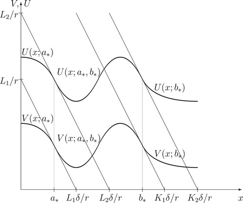
Figure 2. A computer drawing of the value functions $V_{\ast }(x)$ and $U_{\ast }(x)$ and the optimal exercise boundaries $a_{\ast }$ and $b_{\ast }$ in the case $L_1<L_2<K_2<K_1$.

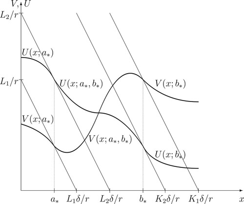
Figure 3. A computer drawing of the value functions $V_{\ast }(x)$ and $U_{\ast }(x)$ and the optimal exercise boundaries $a_{\ast }$ and $b_{\ast }$ in the case $L_2<L_1<K_1<K_2$.

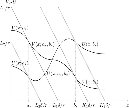
Figure 4. A computer drawing of the value functions $V_{\ast }(x)$ and $U_{\ast }(x)$ and the optimal exercise boundaries $a_{\ast }$ and $b_{\ast }$ in the case $L_2<L_1<K_2<K_1$.

4. Main results and verification

In this section, being based on the facts proved above, we formulate and prove the main result of the paper concerning the nonzero-sum optimal stopping games of (8(8) $\begin{array}{r}{V}_{\ast }(x)=\underset{\tau \in T(\lambda )}{sup}{E}_x[e^{-\mathrm{r\tau }}(\frac{L_1}{r}-\frac{X_{\tau }}{\delta })I(\tau \le {\zeta }_{\ast })+e^{-r{\zeta }_{\ast }}(\frac{K_1}{r}-\frac{X_{{\zeta }_{\ast }}}{\delta })I({\zeta }_{\ast }<\tau )]\end{array}$(8) ) and (9(9) $\begin{array}{r}{U}_{\ast }(x)=\underset{\zeta \in Z(\varkappa )}{inf}{E}_x[e^{-\mathrm{r\zeta }}(\frac{K_2}{r}-\frac{X_{\zeta }}{\delta })I(\zeta \le {\tau }_{\ast })+e^{-r{\tau }_{\ast }}(\frac{L_2}{r}-\frac{X_{{\tau }_{\ast }}}{\delta })I({\tau }_{\ast }<\zeta )]\end{array}$(9) ) with (10(10) $\begin{array}{r}{\overline{V}}_{\ast }(x)=\underset{\tau \in \overline{T}(\lambda )}{sup}{E}_x[e^{-\mathrm{r\tau }}(\frac{L_1}{r}-\frac{X_{\tau }}{\delta })I(\tau \le {\zeta }_{\ast })+e^{-r{\zeta }_{\ast }}(\frac{K_1}{r}-\frac{X_{{\zeta }_{\ast }}}{\delta })I({\zeta }_{\ast }<\tau )]\end{array}$(10) ) and (11(11) $\begin{array}{r}{\overline{U}}_{\ast }(x)=\underset{\zeta \in \overline{Z}(\varkappa )}{inf}{E}_x[e^{-\mathrm{r\zeta }}(\frac{K_2}{r}-\frac{X_{\zeta }}{\delta })I(\zeta \le {\tau }_{\ast })+e^{-r{\tau }_{\ast }}(\frac{L_2}{r}-\frac{X_{{\tau }_{\ast }}}{\delta })I({\tau }_{\ast }<\zeta )]\end{array}$(11) ) in the model defined in (1(1) $\begin{array}{r}{X}_t=\mathrm{xexp}((r-\delta -{\sigma }^2/2)t+\sigma B_t)\end{array}$(1) ) and (2(2) $\begin{array}{r}\mathrm{d}{X}_t=(r-\delta )X_t\mathrm{d}t+\sigma X_t\mathrm{d}{B}_t(X_0=x)\end{array}$(2) ) under Poisson random intervention times. For this purpose, we extend the arguments from [13,25,49] to the case of nonzero-sum optimal stopping games.

Theorem 4.1

Let the process X be defined in (1(1) $\begin{array}{r}{X}_t=\mathrm{xexp}((r-\delta -{\sigma }^2/2)t+\sigma B_t)\end{array}$(1) ) and (2(2) $\begin{array}{r}\mathrm{d}{X}_t=(r-\delta )X_t\mathrm{d}t+\sigma X_t\mathrm{d}{B}_t(X_0=x)\end{array}$(2) ), where r>0, $\delta >0$, and $\sigma >0$ are some given constants. Assume that the couple $a_{\ast }$ and $b_{\ast }$ provides a (possibly multiple) solution of the system of arithmetic power equations in (74(74) $\begin{array}{r}{\left(\frac{b}{a}\right)}^{{\alpha }_1}=\eta (a,b)+\phi (a,b)\mathrm{and}{\left(\frac{b}{a}\right)}^{{\alpha }_2}=\xi (a,b)+\psi (a,b)\end{array}$(74) ) on the intervals $0<a_{\ast }\le L_1$ and $b_{\ast }\ge K_2$, whenever such a solution exists, for the admissible constants $0<L_i<K_j$, for i, j = 1, 2, such that the inequality in (83(83) $\begin{array}{rl}\mathrm{\Delta }(a,b)& \equiv {(F_1(a)H_1(a,b)-F_2(a)H_2(a,b)-(\frac{L_2}{r}-\frac{a}{\delta })\frac{K_1-K_2}{r})}^2\\ & -4F_2(a)H_2(a,b)(\frac{L_2}{r}-\frac{a}{\delta })\frac{K_1-K_2}{r}\ge 0\end{array}$(83) ) is satisfied. Then, the value functions in (8(8) $\begin{array}{r}{V}_{\ast }(x)=\underset{\tau \in T(\lambda )}{sup}{E}_x[e^{-\mathrm{r\tau }}(\frac{L_1}{r}-\frac{X_{\tau }}{\delta })I(\tau \le {\zeta }_{\ast })+e^{-r{\zeta }_{\ast }}(\frac{K_1}{r}-\frac{X_{{\zeta }_{\ast }}}{\delta })I({\zeta }_{\ast }<\tau )]\end{array}$(8) )-(9) and (10)-(11(11) $\begin{array}{r}{\overline{U}}_{\ast }(x)=\underset{\zeta \in \overline{Z}(\varkappa )}{inf}{E}_x[e^{-\mathrm{r\zeta }}(\frac{K_2}{r}-\frac{X_{\zeta }}{\delta })I(\zeta \le {\tau }_{\ast })+e^{-r{\tau }_{\ast }}(\frac{L_2}{r}-\frac{X_{{\tau }_{\ast }}}{\delta })I({\tau }_{\ast }<\zeta )]\end{array}$(11) ) of the perpetual (randomised Bermudian) game-type contingent claim described above with the strikes $0<L_i<K_j$, for every i, j = 1, 2, take the form: (84) $\begin{array}{r}{V}_{\ast }(x)=\{\begin{array}{ll}V(x;a_{\ast }),& \mathrm{if}0<x\le a_{\ast }\\ V(x;a_{\ast },b_{\ast }),& \mathrm{if}{a}_{\ast }<x<b_{\ast }\\ V(x;b_{\ast }),& \mathrm{if}x\ge b_{\ast }\end{array}\end{array}$(84) and (85) $\begin{array}{r}{U}_{\ast }(x)=\{\begin{array}{ll}U(x;a_{\ast }),& \mathrm{if}0<x\le a_{\ast }\\ U(x;a_{\ast },b_{\ast }),& \mathrm{if}{a}_{\ast }<x<b_{\ast }\\ U(x;b_{\ast }),& \mathrm{if}x\ge b_{\ast }\end{array}\end{array}$(85) as well as (86) $\begin{array}{r}{\overline{V}}_{\ast }(x)=\{\begin{array}{ll}{L}_1/r-x/\delta ,& \mathrm{if}0<x\le a_{\ast }\\ V(x;a_{\ast },b_{\ast }),& \mathrm{if}{a}_{\ast }<x<b_{\ast }\\ V(x;b_{\ast }),& \mathrm{if}x\ge b_{\ast }\end{array}\end{array}$(86) and (87) $\begin{array}{r}{\overline{U}}_{\ast }(x)=\{\begin{array}{ll}U(x;a_{\ast }),& \mathrm{if}0<x\le a_{\ast }\\ U(x;a_{\ast },b_{\ast }),& \mathrm{if}{a}_{\ast }<x<b_{\ast }\\ K_2/r-x/\delta ,& \mathrm{if}x\ge b_{\ast }\end{array}\end{array}$(87) respectively. Here, the functions $V(x;a,b)$ and $U(x;a,b)$ are given by (44(44) $\begin{array}{r}V(x;a,b)=A_{1,1}(a,b)x^{{\alpha }_1}+A_{1,2}(a,b)x^{{\alpha }_2}\end{array}$(44) ) and (45(45) $\begin{array}{r}U(x;a,b)=A_{2,1}(a,b)x^{{\alpha }_1}+A_{2,2}(a,b)x^{{\alpha }_2}\end{array}$(45) ) with (46(46) $\begin{array}{r}{A}_{i,j}(a,b)=\frac{(L_i/r-a/\delta )b^{{\alpha }_{3-j}}-(K_i/r-b/\delta )a^{{\alpha }_{3-j}}}{a^{{\alpha }_j}{b}^{{\alpha }_{3-j}}-b^{{\alpha }_j}{a}^{{\alpha }_{3-j}}}\end{array}$(46) ), $V(x;a)$ and $U(x;b)$ are given by (57(57) $\begin{array}{r}V(x;a)=(\frac{L_1}{\lambda +r}-\frac{a}{\lambda +\delta }){\left(\frac{x}{a}\right)}^{{\gamma }_1}+\frac{\lambda L_1}{(\lambda +r)r}-\frac{\mathrm{\lambda x}}{(\lambda +\delta )\delta }\end{array}$(57) ) and (58(58) $\begin{array}{r}U(x;b)=(\frac{K_2}{\varkappa +r}-\frac{b}{\varkappa +\delta }){\left(\frac{x}{b}\right)}^{{\beta }_2}+\frac{\varkappa K_2}{(\varkappa +r)r}-\frac{\mathrm{\varkappa x}}{(\varkappa +\delta )\delta }\end{array}$(58) ), and $V(x;b)$ and $U(x;a)$ are given by (59(59) $\begin{array}{r}V(x;b)=(\frac{K_1}{\varkappa +r}-\frac{b}{\varkappa +\delta }){\left(\frac{x}{b}\right)}^{{\beta }_2}+\frac{\varkappa K_1}{(\varkappa +r)r}-\frac{\mathrm{\varkappa x}}{(\varkappa +\delta )\delta }\end{array}$(59) ) and (60(60) $\begin{array}{r}U(x;a)=(\frac{L_2}{\lambda +r}-\frac{a}{\lambda +\delta }){\left(\frac{x}{a}\right)}^{{\gamma }_1}+\frac{\lambda L_2}{(\lambda +r)r}-\frac{\mathrm{\lambda x}}{(\lambda +\delta )\delta }\end{array}$(60) ) above. Moreover, the optimal exercise times forming Nash equilibria in the games of (8(8) $\begin{array}{r}{V}_{\ast }(x)=\underset{\tau \in T(\lambda )}{sup}{E}_x[e^{-\mathrm{r\tau }}(\frac{L_1}{r}-\frac{X_{\tau }}{\delta })I(\tau \le {\zeta }_{\ast })+e^{-r{\zeta }_{\ast }}(\frac{K_1}{r}-\frac{X_{{\zeta }_{\ast }}}{\delta })I({\zeta }_{\ast }<\tau )]\end{array}$(8) )-(9) and (10)-(11(11) $\begin{array}{r}{\overline{U}}_{\ast }(x)=\underset{\zeta \in \overline{Z}(\varkappa )}{inf}{E}_x[e^{-\mathrm{r\zeta }}(\frac{K_2}{r}-\frac{X_{\zeta }}{\delta })I(\zeta \le {\tau }_{\ast })+e^{-r{\tau }_{\ast }}(\frac{L_2}{r}-\frac{X_{{\tau }_{\ast }}}{\delta })I({\tau }_{\ast }<\zeta )]\end{array}$(11) ) are given by: (88) $\begin{array}{r}{\tau }_{\ast }=inf\{{\tau }_n\in T(\lambda )|X_{{\tau }_n}\le a_{\ast },n\in \mathbb{N}\}\mathrm{and}{\zeta }_{\ast }=inf\{{\zeta }_n\in Z(\varkappa )|X_{{\zeta }_n}\ge b_{\ast },n\in \mathbb{N}\}\end{array}$(88) as well as (89) $\begin{array}{r}{\overline{\tau }}_{\ast }=inf\{{\tau }_n\in \overline{T}(\lambda )|X_{{\tau }_n}\le a_{\ast },n\in \overline{\mathbb{N}}\}\mathrm{and}{\overline{\zeta }}_{\ast }=inf\{{\zeta }_n\in \overline{Z}(\varkappa )|X_{{\zeta }_n}\ge b_{\ast },n\in \overline{\mathbb{N}}\}\end{array}$(89) respectively.

Proof.

In order to verify the assertion stated above, it remains for us to show that the functions defined in (84(84) $\begin{array}{r}{V}_{\ast }(x)=\{\begin{array}{ll}V(x;a_{\ast }),& \mathrm{if}0<x\le a_{\ast }\\ V(x;a_{\ast },b_{\ast }),& \mathrm{if}{a}_{\ast }<x<b_{\ast }\\ V(x;b_{\ast }),& \mathrm{if}x\ge b_{\ast }\end{array}\end{array}$(84) )-(85) and (86)-(87(87) $\begin{array}{r}{\overline{U}}_{\ast }(x)=\{\begin{array}{ll}U(x;a_{\ast }),& \mathrm{if}0<x\le a_{\ast }\\ U(x;a_{\ast },b_{\ast }),& \mathrm{if}{a}_{\ast }<x<b_{\ast }\\ K_2/r-x/\delta ,& \mathrm{if}x\ge b_{\ast }\end{array}\end{array}$(87) ) coincide with the value functions in (8(8) $\begin{array}{r}{V}_{\ast }(x)=\underset{\tau \in T(\lambda )}{sup}{E}_x[e^{-\mathrm{r\tau }}(\frac{L_1}{r}-\frac{X_{\tau }}{\delta })I(\tau \le {\zeta }_{\ast })+e^{-r{\zeta }_{\ast }}(\frac{K_1}{r}-\frac{X_{{\zeta }_{\ast }}}{\delta })I({\zeta }_{\ast }<\tau )]\end{array}$(8) )-(9) and (10)-(11(11) $\begin{array}{r}{\overline{U}}_{\ast }(x)=\underset{\zeta \in \overline{Z}(\varkappa )}{inf}{E}_x[e^{-\mathrm{r\zeta }}(\frac{K_2}{r}-\frac{X_{\zeta }}{\delta })I(\zeta \le {\tau }_{\ast })+e^{-r{\tau }_{\ast }}(\frac{L_2}{r}-\frac{X_{{\tau }_{\ast }}}{\delta })I({\tau }_{\ast }<\zeta )]\end{array}$(11) ), respectively, while the stopping times ${\tau }_{\ast }$ and ${\zeta }_{\ast }$ in (88(88) $\begin{array}{r}{\tau }_{\ast }=inf\{{\tau }_n\in T(\lambda )|X_{{\tau }_n}\le a_{\ast },n\in \mathbb{N}\}\mathrm{and}{\zeta }_{\ast }=inf\{{\zeta }_n\in Z(\varkappa )|X_{{\zeta }_n}\ge b_{\ast },n\in \mathbb{N}\}\end{array}$(88) ) as well as ${\overline{\tau }}_{\ast }$ and ${\overline{\zeta }}_{\ast }$ in (89(89) $\begin{array}{r}{\overline{\tau }}_{\ast }=inf\{{\tau }_n\in \overline{T}(\lambda )|X_{{\tau }_n}\le a_{\ast },n\in \overline{\mathbb{N}}\}\mathrm{and}{\overline{\zeta }}_{\ast }=inf\{{\zeta }_n\in \overline{Z}(\varkappa )|X_{{\zeta }_n}\ge b_{\ast },n\in \overline{\mathbb{N}}\}\end{array}$(89) ) form a Nash equilibrium there with the boundaries $a_{\ast }$ and $b_{\ast }$ specified in the previous section. For this purpose, let us denote by $V(x)$ and $U(x)$ as well as $\overline{V}(x)$ and $\overline{U}(x)$ the right-hand sides of the expressions in (84(84) $\begin{array}{r}{V}_{\ast }(x)=\{\begin{array}{ll}V(x;a_{\ast }),& \mathrm{if}0<x\le a_{\ast }\\ V(x;a_{\ast },b_{\ast }),& \mathrm{if}{a}_{\ast }<x<b_{\ast }\\ V(x;b_{\ast }),& \mathrm{if}x\ge b_{\ast }\end{array}\end{array}$(84) ) and (85(85) $\begin{array}{r}{U}_{\ast }(x)=\{\begin{array}{ll}U(x;a_{\ast }),& \mathrm{if}0<x\le a_{\ast }\\ U(x;a_{\ast },b_{\ast }),& \mathrm{if}{a}_{\ast }<x<b_{\ast }\\ U(x;b_{\ast }),& \mathrm{if}x\ge b_{\ast }\end{array}\end{array}$(85) ) as well as (86(86) $\begin{array}{r}{\overline{V}}_{\ast }(x)=\{\begin{array}{ll}{L}_1/r-x/\delta ,& \mathrm{if}0<x\le a_{\ast }\\ V(x;a_{\ast },b_{\ast }),& \mathrm{if}{a}_{\ast }<x<b_{\ast }\\ V(x;b_{\ast }),& \mathrm{if}x\ge b_{\ast }\end{array}\end{array}$(86) ) and (87(87) $\begin{array}{r}{\overline{U}}_{\ast }(x)=\{\begin{array}{ll}U(x;a_{\ast }),& \mathrm{if}0<x\le a_{\ast }\\ U(x;a_{\ast },b_{\ast }),& \mathrm{if}{a}_{\ast }<x<b_{\ast }\\ K_2/r-x/\delta ,& \mathrm{if}x\ge b_{\ast }\end{array}\end{array}$(87) ) associated with these boundaries $a_{\ast }$ and $b_{\ast }$, respectively.

(i) It follows from the straightforward calculations presented in the previous section that the functions $V(x)$ and $U(x)$ solve the system of (30(30) $\begin{array}{rl}& (\mathbb{L}V-(r+\lambda )V)(x)+\frac{\lambda L_1}{r}-\frac{\mathrm{\lambda x}}{\delta }=0\mathrm{for}x<a\mathrm{and}\end{array}$(30) )–(39(39) $\begin{array}{rl}& V(x)<\frac{L_1}{r}-\frac{x}{\delta }\mathrm{for}x<a\mathrm{and}U(x)>\frac{K_2}{r}-\frac{x}{\delta }\mathrm{for}x>b\end{array}$(39) ). We also observe from the constructions of the previous section that the function $V(x)$ is $C^2$ in $(0,b_{\ast }]$ and $[b_{\ast },\mathrm{\infty })$ as well as $C^1$ at the point $b_{\ast }$, while the function $U(x)$ is $C^2$ in $[a_{\ast },\mathrm{\infty })$ and $(0,a_{\ast }]$ as well as $C^1$ at the point $a_{\ast }$. Then, by applying the local time-space formula from [44] (see also [47, Chapter II, Section 3.5] for a summary of the related results and further references) to the processes $e^{-(r+\lambda )t}V(X_t)$ and $e^{-(r+\varkappa )t}U(X_t)$, we obtain: (90) $\begin{array}{r}{e}^{-(r+\lambda )t}V(X_t)=V(x)+{\int }_0^t{e}^{-(r+\lambda )u}(\mathbb{L}V-(r+\lambda )V)(X_u)I(X_u\ne b_{\ast })\mathrm{d}u+M_t^1\end{array}$(90) and (91) $\begin{array}{r}{e}^{-(r+\varkappa )t}U(X_t)=U(x)+{\int }_0^t{e}^{-(r+\varkappa )u}(\mathbb{L}U-(r+\varkappa )U)(X_u)I(X_u\ne a_{\ast })\mathrm{d}u+M_t^2\end{array}$(91) for all $t\ge 0$. Here, by virtue of the properties indicated in the previous section that the functions $V(x)$ and $U(x)$ are at least $C^1$ on $(0,\mathrm{\infty })$, there are no local time terms in the expressions of (90(90) $\begin{array}{r}{e}^{-(r+\lambda )t}V(X_t)=V(x)+{\int }_0^t{e}^{-(r+\lambda )u}(\mathbb{L}V-(r+\lambda )V)(X_u)I(X_u\ne b_{\ast })\mathrm{d}u+M_t^1\end{array}$(90) ) and (91(91) $\begin{array}{r}{e}^{-(r+\varkappa )t}U(X_t)=U(x)+{\int }_0^t{e}^{-(r+\varkappa )u}(\mathbb{L}U-(r+\varkappa )U)(X_u)I(X_u\ne a_{\ast })\mathrm{d}u+M_t^2\end{array}$(91) ), while the processes $M^i=(M_t^i{)}_{t\ge 0}$, for i = 1, 2, defined by: (92) $\begin{array}{r}{M}_t^1={\int }_0^t{e}^{-(r+\lambda )u}{V}^{\prime }(X_u)\sigma X_u\mathrm{d}{B}_u\mathrm{and}{M}_t^2={\int }_0^t{e}^{-(r+\varkappa )u}{U}^{\prime }(X_u)\sigma X_u\mathrm{d}{B}_u\end{array}$(92) are continuous local martingales under the probability measure $P_x$. Observe from the arguments of the previous section that the derivatives $V^{\prime }(x)$ and $U^{\prime }(x)$ are bounded functions, so that the processes $M^i$, for i = 1, 2, from (92(92) $\begin{array}{r}{M}_t^1={\int }_0^t{e}^{-(r+\lambda )u}{V}^{\prime }(X_u)\sigma X_u\mathrm{d}{B}_u\mathrm{and}{M}_t^2={\int }_0^t{e}^{-(r+\varkappa )u}{U}^{\prime }(X_u)\sigma X_u\mathrm{d}{B}_u\end{array}$(92) ) are continuous square integrable martingales. Note that, since the time spent by the process X at the boundaries $a_{\ast }$ and $b_{\ast }$ is of the Lebesgue measure zero (see, e.g. [10, Chapter II, Section 1]), the indicators in the formulas of (90(90) $\begin{array}{r}{e}^{-(r+\lambda )t}V(X_t)=V(x)+{\int }_0^t{e}^{-(r+\lambda )u}(\mathbb{L}V-(r+\lambda )V)(X_u)I(X_u\ne b_{\ast })\mathrm{d}u+M_t^1\end{array}$(90) ) and (91(91) $\begin{array}{r}{e}^{-(r+\varkappa )t}U(X_t)=U(x)+{\int }_0^t{e}^{-(r+\varkappa )u}(\mathbb{L}U-(r+\varkappa )U)(X_u)I(X_u\ne a_{\ast })\mathrm{d}u+M_t^2\end{array}$(91) ) can be set equal to one. Moreover, it also follows from the straightforward calculations of the previous section that the equality $(\mathbb{L}V-(r+\lambda )V)(x)=-\lambda \overline{V}(x)$ holds, for all x>0 such that $x\ne b_{\ast }$, while the equality $(\mathbb{L}U-(r+\varkappa )U)(x)=-\varkappa \overline{U}(x)$ holds, for all x>0 such that $x\ne a_{\ast }$. Hence, by applying the Lebesgue dominated convergence theorem to the expressions in (90(90) $\begin{array}{r}{e}^{-(r+\lambda )t}V(X_t)=V(x)+{\int }_0^t{e}^{-(r+\lambda )u}(\mathbb{L}V-(r+\lambda )V)(X_u)I(X_u\ne b_{\ast })\mathrm{d}u+M_t^1\end{array}$(90) ) and (91(91) $\begin{array}{r}{e}^{-(r+\varkappa )t}U(X_t)=U(x)+{\int }_0^t{e}^{-(r+\varkappa )u}(\mathbb{L}U-(r+\varkappa )U)(X_u)I(X_u\ne a_{\ast })\mathrm{d}u+M_t^2\end{array}$(91) ), we obtain that the equalities: (93) $\begin{array}{r}V(x)=E_x[e^{-r{\tau }_1}\overline{V}(X_{{\tau }_1})I({\tau }_1\le {\zeta }_{\ast })+e^{-r{\zeta }_{\ast }}(\overline{U}(X_{{\zeta }_{\ast }})-\frac{K_2-K_1}{r})I({\zeta }_{\ast }<{\tau }_1)]\end{array}$(93) and (94) $\begin{array}{r}U(x)=E_x[e^{-r{\zeta }_1}\overline{U}(X_{{\zeta }_1})I({\zeta }_1\le {\tau }_{\ast })+e^{-r{\tau }_{\ast }}(\overline{V}(X_{{\tau }_{\ast }})-\frac{L_1-L_2}{r})I({\tau }_{\ast }<{\zeta }_1)]\end{array}$(94) hold, for all x>0.

(ii) Let us now show that the candidate functions $\overline{V}(x)$ and $\overline{U}(x)$ coincide with the value functions ${\overline{V}}_{\ast }(x)$ and ${\overline{U}}_{\ast }(x)$ and the stopping times ${\overline{\tau }}_{\ast }$ and ${\overline{\zeta }}_{\ast }$ from (89(89) $\begin{array}{r}{\overline{\tau }}_{\ast }=inf\{{\tau }_n\in \overline{T}(\lambda )|X_{{\tau }_n}\le a_{\ast },n\in \overline{\mathbb{N}}\}\mathrm{and}{\overline{\zeta }}_{\ast }=inf\{{\zeta }_n\in \overline{Z}(\varkappa )|X_{{\zeta }_n}\ge b_{\ast },n\in \overline{\mathbb{N}}\}\end{array}$(89) ) are optimal (forming a Nash equilibrium) in the problem of (10(10) $\begin{array}{r}{\overline{V}}_{\ast }(x)=\underset{\tau \in \overline{T}(\lambda )}{sup}{E}_x[e^{-\mathrm{r\tau }}(\frac{L_1}{r}-\frac{X_{\tau }}{\delta })I(\tau \le {\zeta }_{\ast })+e^{-r{\zeta }_{\ast }}(\frac{K_1}{r}-\frac{X_{{\zeta }_{\ast }}}{\delta })I({\zeta }_{\ast }<\tau )]\end{array}$(10) ) and (11(11) $\begin{array}{r}{\overline{U}}_{\ast }(x)=\underset{\zeta \in \overline{Z}(\varkappa )}{inf}{E}_x[e^{-\mathrm{r\zeta }}(\frac{K_2}{r}-\frac{X_{\zeta }}{\delta })I(\zeta \le {\tau }_{\ast })+e^{-r{\tau }_{\ast }}(\frac{L_2}{r}-\frac{X_{{\tau }_{\ast }}}{\delta })I({\tau }_{\ast }<\zeta )]\end{array}$(11) ). For this purpose, we first observe that the inequalities: (95) $\begin{array}{r}\overline{V}(x)\ge V(x)=E_x[e^{-r{\tau }_1}\overline{V}(X_{{\tau }_1})I({\tau }_1\le {\zeta }_{\ast })+e^{-r{\zeta }_{\ast }}(\overline{U}(X_{{\zeta }_{\ast }})-\frac{K_2-K_1}{r})I({\zeta }_{\ast }<{\tau }_1)]\end{array}$(95) and (96) $\begin{array}{r}\overline{U}(x)\le U(x)=E_x[e^{-r{\zeta }_1}\overline{U}(X_{{\zeta }_1})I({\zeta }_1\le {\tau }_{\ast })+e^{-r{\tau }_{\ast }}(\overline{V}(X_{{\tau }_{\ast }})-\frac{L_1-L_2}{r})I({\tau }_{\ast }<{\zeta }_1)]\end{array}$(96) hold, where ${\tau }_1$ and ${\zeta }_1$ are independent of each other and of the driving standard Brownian motion B exponential random variables with the means $1/\lambda$ and $1/\varkappa$, respectively. These facts imply that the processes $(e^{-r({\tau }_l\wedge {\zeta }_{\ast })}\overline{V}(X_{{\tau }_l\wedge {\zeta }_{\ast }}){)}_{l\in \overline{\mathbb{N}}}$ and $(e^{-r({\tau }_{\ast }\wedge {\zeta }_k)}\overline{U}(X_{{\tau }_{\ast }\wedge {\zeta }_k}){)}_{k\in \overline{\mathbb{N}}}$ are discrete-time nonnegative bounded supermartingale and submartingale under the probability measure $P_x$, respectively. Then, taking into account the strong Markov property of the process X as well as stationarity and independence of increments of the processes $N^i$, for i = 1, 2, it follows from Doob's optional sampling theorem that the inequalities: (97) $\begin{array}{rl}\overline{V}(x)& \ge E_x[e^{-\mathrm{r\tau }}\overline{V}(X_{\tau })I(\tau \le {\zeta }_{\ast })+e^{-r{\zeta }_{\ast }}(\overline{U}(X_{{\zeta }_{\ast }})-\frac{K_2-K_1}{r})I({\zeta }_{\ast }<\tau )]\\ & \ge E_x[e^{-\mathrm{r\tau }}(\frac{L_1}{r}-\frac{X_{\tau }}{\delta })I(\tau \le {\zeta }_{\ast })+e^{-r{\zeta }_{\ast }}(\frac{K_1}{r}-\frac{X_{{\zeta }_{\ast }}}{\delta })I({\zeta }_{\ast }<\tau )]\end{array}$(97) and (98) $\begin{array}{rl}\overline{U}(x)& \le E_x[e^{-\mathrm{r\zeta }}\overline{U}(X_{\zeta })I(\zeta \le {\tau }_{\ast })+e^{-r{\tau }_{\ast }}(\overline{V}(X_{{\tau }_{\ast }})-\frac{L_1-L_2}{r})I({\tau }_{\ast }<\zeta )]\\ & \le E_x[e^{-\mathrm{r\zeta }}(\frac{K_2}{r}-\frac{X_{\zeta }}{\delta })I(\zeta \le {\tau }_{\ast })+e^{-r{\overline{\tau }}_{\ast }}(\frac{L_2}{r}-\frac{X_{{\overline{\tau }}_{\ast }}}{\delta })I({\tau }_{\ast }<\zeta )]\end{array}$(98) hold, for any stopping times τ and ζ with respect to the filtrations $({\mathcal{G}}_{{\tau }_l}{)}_{l\in \overline{\mathbb{N}}}$ and $({\mathcal{H}}_{{\zeta }_k}{)}_{k\in \overline{\mathbb{N}}}$, respectively. Hence, after taking the supremum and infimum over τ and ζ from the sets $\overline{T}(\lambda )$ and $\overline{Z}(\varkappa )$, we get that the inequalities $\overline{V}(x)\ge {\overline{V}}_{\ast }(x)$ and $\overline{U}(x)\le {\overline{U}}_{\ast }(x)$ hold, for all x>0. On the other hand, let us recall that the well-known property: (99) $\begin{array}{r}{E}_x[\underset{t\ge 0}{sup}{e}^{-\mathrm{rt}}{X}_t]<\mathrm{\infty }\end{array}$(99) holds, for all x>0 (see, e.g. [52, Chapter VIII, Section 2a]). In this respect, we may conclude that the processes $(e^{-r({\tau }_l\wedge {\overline{\tau }}_{\ast }\wedge {\zeta }_{\ast })}\overline{V}(X_{{\tau }_l\wedge {\overline{\tau }}_{\ast }\wedge {\zeta }_{\ast }}){)}_{l\in \overline{\mathbb{N}}}$ and $(e^{-r({\tau }_{\ast }\wedge {\zeta }_k\wedge {\overline{\zeta }}_{\ast })}\overline{U}(X_{{\tau }_{\ast }\wedge {\zeta }_k\wedge {\overline{\zeta }}_{\ast }}){)}_{k\in \overline{\mathbb{N}}}$ are discrete-time nonnegative bounded uniformly integrable martingales. Therefore, by applying the Lebesgue dominated convergence theorem to the expressions in (97(97) $\begin{array}{rl}\overline{V}(x)& \ge E_x[e^{-\mathrm{r\tau }}\overline{V}(X_{\tau })I(\tau \le {\zeta }_{\ast })+e^{-r{\zeta }_{\ast }}(\overline{U}(X_{{\zeta }_{\ast }})-\frac{K_2-K_1}{r})I({\zeta }_{\ast }<\tau )]\\ & \ge E_x[e^{-\mathrm{r\tau }}(\frac{L_1}{r}-\frac{X_{\tau }}{\delta })I(\tau \le {\zeta }_{\ast })+e^{-r{\zeta }_{\ast }}(\frac{K_1}{r}-\frac{X_{{\zeta }_{\ast }}}{\delta })I({\zeta }_{\ast }<\tau )]\end{array}$(97) ) and (98(98) $\begin{array}{rl}\overline{U}(x)& \le E_x[e^{-\mathrm{r\zeta }}\overline{U}(X_{\zeta })I(\zeta \le {\tau }_{\ast })+e^{-r{\tau }_{\ast }}(\overline{V}(X_{{\tau }_{\ast }})-\frac{L_1-L_2}{r})I({\tau }_{\ast }<\zeta )]\\ & \le E_x[e^{-\mathrm{r\zeta }}(\frac{K_2}{r}-\frac{X_{\zeta }}{\delta })I(\zeta \le {\tau }_{\ast })+e^{-r{\overline{\tau }}_{\ast }}(\frac{L_2}{r}-\frac{X_{{\overline{\tau }}_{\ast }}}{\delta })I({\tau }_{\ast }<\zeta )]\end{array}$(98) ), we obtain that the equalities: (100) $\begin{array}{r}\overline{V}(x)=E_x[e^{-r{\overline{\tau }}_{\ast }}(\frac{L_1}{r}-\frac{X_{{\overline{\tau }}_{\ast }}}{\delta })I({\overline{\tau }}_{\ast }\le {\zeta }_{\ast })+e^{-r{\zeta }_{\ast }}(\frac{K_1}{r}-\frac{X_{{\zeta }_{\ast }}}{\delta })I({\zeta }_{\ast }<{\overline{\tau }}_{\ast })]\end{array}$(100) and (101) $\begin{array}{r}\overline{U}(x)=E_x[e^{-r{\overline{\zeta }}_{\ast }}(\frac{K_2}{r}-\frac{X_{{\overline{\zeta }}_{\ast }}}{\delta })I({\overline{\zeta }}_{\ast }\le {\tau }_{\ast })+e^{-r{\tau }_{\ast }}(\frac{L_2}{r}-\frac{X_{{\tau }_{\ast }}}{\delta })I({\tau }_{\ast }<{\overline{\zeta }}_{\ast })]\end{array}$(101) are attained, for the stopping times ${\overline{\tau }}_{\ast }$ and ${\overline{\zeta }}_{\ast }$ from (89(89) $\begin{array}{r}{\overline{\tau }}_{\ast }=inf\{{\tau }_n\in \overline{T}(\lambda )|X_{{\tau }_n}\le a_{\ast },n\in \overline{\mathbb{N}}\}\mathrm{and}{\overline{\zeta }}_{\ast }=inf\{{\zeta }_n\in \overline{Z}(\varkappa )|X_{{\zeta }_n}\ge b_{\ast },n\in \overline{\mathbb{N}}\}\end{array}$(89) ), thus proving the claim.

(iii) Finally, we show that the candidate functions $V(x)$ and $U(x)$ coincide with the value functions $V_{\ast }(x)$ and $U_{\ast }(x)$ and the stopping times ${\tau }_{\ast }$ and ${\zeta }_{\ast }$ from (88(88) $\begin{array}{r}{\tau }_{\ast }=inf\{{\tau }_n\in T(\lambda )|X_{{\tau }_n}\le a_{\ast },n\in \mathbb{N}\}\mathrm{and}{\zeta }_{\ast }=inf\{{\zeta }_n\in Z(\varkappa )|X_{{\zeta }_n}\ge b_{\ast },n\in \mathbb{N}\}\end{array}$(88) ) are optimal (forming a Nash equilibrium) in the problem of (8(8) $\begin{array}{r}{V}_{\ast }(x)=\underset{\tau \in T(\lambda )}{sup}{E}_x[e^{-\mathrm{r\tau }}(\frac{L_1}{r}-\frac{X_{\tau }}{\delta })I(\tau \le {\zeta }_{\ast })+e^{-r{\zeta }_{\ast }}(\frac{K_1}{r}-\frac{X_{{\zeta }_{\ast }}}{\delta })I({\zeta }_{\ast }<\tau )]\end{array}$(8) ) and (9(9) $\begin{array}{r}{U}_{\ast }(x)=\underset{\zeta \in Z(\varkappa )}{inf}{E}_x[e^{-\mathrm{r\zeta }}(\frac{K_2}{r}-\frac{X_{\zeta }}{\delta })I(\zeta \le {\tau }_{\ast })+e^{-r{\tau }_{\ast }}(\frac{L_2}{r}-\frac{X_{{\tau }_{\ast }}}{\delta })I({\tau }_{\ast }<\zeta )]\end{array}$(9) ). For this purpose, we use the fact similar to the one proved in Part (ii) above that the processes $(e^{-r({\tau }_l\wedge {\zeta }_{\ast })}\overline{V}(X_{{\tau }_l\wedge {\zeta }_{\ast }}){)}_{l\in \mathbb{N}}$ and $(e^{-r({\tau }_{\ast }\wedge {\zeta }_k)}\overline{U}(X_{{\tau }_{\ast }\wedge {\zeta }_k}){)}_{k\in \mathbb{N}}$ are discrete-time nonnegative bounded supermartingale and submartingale under the probability measure $P_x$, respectively. Then, we have that the equalities: (102) $\begin{array}{rl}V(x)& =E_x[e^{-r{\tau }_1}\overline{V}(X_{{\tau }_1})I({\tau }_1\le {\zeta }_{\ast })+e^{-r{\zeta }_{\ast }}(\overline{U}(X_{{\zeta }_{\ast }})-\frac{K_2-K_1}{r})I({\zeta }_{\ast }<{\tau }_1)]\\ & \ge E_x[e^{-\mathrm{r\tau }}(\frac{L_1}{r}-\frac{X_{\tau }}{\delta })I(\tau \le {\zeta }_{\ast })+e^{-r{\zeta }_{\ast }}(\frac{K_1}{r}-\frac{X_{{\zeta }_{\ast }}}{\delta })I({\zeta }_{\ast }<\tau )]\end{array}$(102) and (103) $\begin{array}{rl}U(x)& =E_x[e^{-r{\zeta }_1}\overline{U}(X_{{\zeta }_1})I({\zeta }_1\le {\tau }_{\ast })+e^{-r{\tau }_{\ast }}(\overline{V}(X_{{\tau }_{\ast }})-\frac{L_1-L_2}{r})I({\tau }_{\ast }<{\zeta }_1)]\end{array}$(103) (104) $\begin{array}{rl}& \le E_x[e^{-\mathrm{r\zeta }}(\frac{K_2}{r}-\frac{X_{\zeta }}{\delta })I(\zeta \le {\tau }_{\ast })+e^{-r{\tau }_{\ast }}(\frac{L_2}{r}-\frac{X_{{\tau }_{\ast }}}{\delta })I({\tau }_{\ast }<\zeta )]\end{array}$(104) hold, for any stopping times τ and ζ with respect to the filtrations $({\mathcal{G}}_{{\tau }_l}{)}_{l\in \mathbb{N}}$ and $({\mathcal{H}}_{{\zeta }_k}{)}_{k\in \mathbb{N}}$, respectively. Hence, after taking the supremum and infimum over τ and ζ from the sets $T(\lambda )$ and $Z(\varkappa )$, we get that the inequalities $V(x)\ge V_{\ast }(x)$ and $U(x)\le U_{\ast }(x)$ hold, for all x>0. However, conditioning on the first jump times ${\tau }_1$ and ${\zeta }_1$ of the processes $N^i$, for i = 1, 2, by virtue of the strong Markov property of the process X as well as stationarity and independence of increments of the processes $N^i$, for i = 1, 2, we obtain that the equalities: (105) $\begin{array}{rl}V(x)& =E_x[e^{-r{\tau }_1}\overline{V}(X_{{\tau }_1})I({\tau }_1\le {\zeta }_{\ast })+e^{-r{\zeta }_{\ast }}(\overline{U}(X_{{\zeta }_{\ast }})-\frac{K_2-K_1}{r})I({\zeta }_{\ast }<{\tau }_1)]\\ & =E_x[{\int }_0^{\mathrm{\infty }}{e}^{-\mathrm{rt}}{E}_{X_t}[e^{-r{\overline{\tau }}_{\ast }}(\frac{L_1}{r}-\frac{X_{{\overline{\tau }}_{\ast }}}{\delta })I({\overline{\tau }}_{\ast }\le {\zeta }_{\ast })\\ & +e^{-r{\zeta }_{\ast }}(\frac{K_1}{r}-\frac{X_{{\zeta }_{\ast }}}{\delta })I({\zeta }_{\ast }<{\overline{\tau }}_{\ast })]\lambda e^{-\mathrm{\lambda t}}\mathrm{d}t]\\ & ={\int }_0^{\mathrm{\infty }}{E}_x[e^{-r{\tau }_{\ast }}(\frac{L_1}{r}-\frac{X_{{\tau }_{\ast }}}{\delta })I({\tau }_{\ast }\le {\zeta }_{\ast })\\ & +e^{-r{\zeta }_{\ast }}(\frac{K_1}{r}-\frac{X_{{\zeta }_{\ast }}}{\delta })I({\zeta }_{\ast }<{\tau }_{\ast })|{\tau }_1=t]\lambda e^{-\mathrm{\lambda t}}\mathrm{d}t\\ & =E_x[e^{-r{\tau }_{\ast }}(\frac{L_1}{r}-\frac{X_{{\tau }_{\ast }}}{\delta })I({\tau }_{\ast }\le {\zeta }_{\ast })+e^{-r{\zeta }_{\ast }}(\frac{K_1}{r}-\frac{X_{{\zeta }_{\ast }}}{\delta })I({\zeta }_{\ast }<{\tau }_{\ast })]\end{array}$(105) and (106) $\begin{array}{rl}U(x)& =E_x[e^{-r{\zeta }_1}\overline{U}(X_{{\zeta }_1})I({\zeta }_1\le {\tau }_{\ast })+e^{-r{\tau }_{\ast }}(\overline{V}(X_{{\tau }_{\ast }})-\frac{L_1-L_2}{r})I({\tau }_{\ast }<{\zeta }_1)]\\ & =E_x[{\int }_0^{\mathrm{\infty }}{e}^{-\mathrm{rt}}{E}_{X_t}[e^{-r{\overline{\zeta }}_{\ast }}(\frac{K_2}{r}-\frac{X_{{\overline{\zeta }}_{\ast }}}{\delta })I({\overline{\zeta }}_{\ast }\le {\tau }_{\ast })\\ & +e^{-r{\tau }_{\ast }}(\frac{L_2}{r}-\frac{X_{{\tau }_{\ast }}}{\delta })I({\tau }_{\ast }<{\overline{\zeta }}_{\ast })]\varkappa e^{-\mathrm{\varkappa t}}\mathrm{d}t]\\ & ={\int }_0^{\mathrm{\infty }}{E}_x[e^{-r{\zeta }_{\ast }}(\frac{K_2}{r}-\frac{X_{{\zeta }_{\ast }}}{\delta })I({\zeta }_{\ast }\le {\tau }_{\ast })\\ & +e^{-r{\tau }_{\ast }}(\frac{L_2}{r}-\frac{X_{{\tau }_{\ast }}}{\delta })I({\tau }_{\ast }<{\zeta }_{\ast })|{\zeta }_1=t]\varkappa e^{-\mathrm{\varkappa t}}\mathrm{d}t\\ & =E_x[e^{-r{\zeta }_{\ast }}(\frac{K_2}{r}-\frac{X_{{\zeta }_{\ast }}}{\delta })I({\zeta }_{\ast }\le {\tau }_{\ast })+e^{-r{\tau }_{\ast }}(\frac{L_2}{r}-\frac{X_{{\tau }_{\ast }}}{\delta })I({\tau }_{\ast }<{\zeta }_{\ast })]\end{array}$(106) are attained, at the stopping times ${\tau }_{\ast }$ and ${\zeta }_{\ast }$ from (88(88) $\begin{array}{r}{\tau }_{\ast }=inf\{{\tau }_n\in T(\lambda )|X_{{\tau }_n}\le a_{\ast },n\in \mathbb{N}\}\mathrm{and}{\zeta }_{\ast }=inf\{{\zeta }_n\in Z(\varkappa )|X_{{\zeta }_n}\ge b_{\ast },n\in \mathbb{N}\}\end{array}$(88) ), thus proving the claim.

5. Convergence to the classical case

In this section, we will show that the solution to the nonzero-sum optimal stopping game under random Poisson intervention times presented in (84(84) $\begin{array}{r}{V}_{\ast }(x)=\{\begin{array}{ll}V(x;a_{\ast }),& \mathrm{if}0<x\le a_{\ast }\\ V(x;a_{\ast },b_{\ast }),& \mathrm{if}{a}_{\ast }<x<b_{\ast }\\ V(x;b_{\ast }),& \mathrm{if}x\ge b_{\ast }\end{array}\end{array}$(84) )-(85(85) $\begin{array}{r}{U}_{\ast }(x)=\{\begin{array}{ll}U(x;a_{\ast }),& \mathrm{if}0<x\le a_{\ast }\\ U(x;a_{\ast },b_{\ast }),& \mathrm{if}{a}_{\ast }<x<b_{\ast }\\ U(x;b_{\ast }),& \mathrm{if}x\ge b_{\ast }\end{array}\end{array}$(85) ) with (86(86) $\begin{array}{r}{\overline{V}}_{\ast }(x)=\{\begin{array}{ll}{L}_1/r-x/\delta ,& \mathrm{if}0<x\le a_{\ast }\\ V(x;a_{\ast },b_{\ast }),& \mathrm{if}{a}_{\ast }<x<b_{\ast }\\ V(x;b_{\ast }),& \mathrm{if}x\ge b_{\ast }\end{array}\end{array}$(86) )-(87) and (88)-(89(89) $\begin{array}{r}{\overline{\tau }}_{\ast }=inf\{{\tau }_n\in \overline{T}(\lambda )|X_{{\tau }_n}\le a_{\ast },n\in \overline{\mathbb{N}}\}\mathrm{and}{\overline{\zeta }}_{\ast }=inf\{{\zeta }_n\in \overline{Z}(\varkappa )|X_{{\zeta }_n}\ge b_{\ast },n\in \overline{\mathbb{N}}\}\end{array}$(89) ) converges to the solution of the associated nonzero-sum optimal stopping game under continuous observations as the intensities of the Poisson processes tend to infinity. For this purpose, we first formulate the associated nonzero-sum optimal stopping games with the same total expected reward functionals from (3(3) $\begin{array}{r}{J}_1(\tau ,\zeta )=E[{\int }_0^{\tau \wedge \zeta }{e}^{-\mathrm{rs}}{X}_s\mathrm{d}s+e^{-\mathrm{r\tau }}\frac{L_1}{r}I(\tau \le \zeta )+e^{-\mathrm{r\zeta }}\frac{K_1}{r}I(\zeta <\tau )]\end{array}$(3) ) and (4(4) $\begin{array}{r}{J}_2(\zeta ,\tau )=E[{\int }_0^{\tau \wedge \zeta }{e}^{-\mathrm{rs}}{X}_s\mathrm{d}s+e^{-\mathrm{r\zeta }}\frac{K_2}{r}I(\zeta \le \tau )+e^{-\mathrm{r\tau }}\frac{L_2}{r}I(\tau <\zeta )]\end{array}$(4) ) and such that the inequalities: (107) $\begin{array}{r}{J}_1(\tau ,\hat{\zeta })\le J_1(\hat{\tau },\hat{\zeta })\mathrm{and}{J}_2(\hat{\zeta },\hat{\tau })\le J_2(\zeta ,\hat{\tau })\end{array}$(107) should hold, for any stopping times τ and ζ from the set S of all stopping times with respect to the filtration $({\mathcal{F}}_t{)}_{t\ge 0}$ generated by the process X. Such a couple $\hat{\tau }$ and $\hat{\zeta }$ satisfying the inequalities in (107(107) $\begin{array}{r}{J}_1(\tau ,\hat{\zeta })\le J_1(\hat{\tau },\hat{\zeta })\mathrm{and}{J}_2(\hat{\zeta },\hat{\tau })\le J_2(\zeta ,\hat{\tau })\end{array}$(107) ) with (3(3) $\begin{array}{r}{J}_1(\tau ,\zeta )=E[{\int }_0^{\tau \wedge \zeta }{e}^{-\mathrm{rs}}{X}_s\mathrm{d}s+e^{-\mathrm{r\tau }}\frac{L_1}{r}I(\tau \le \zeta )+e^{-\mathrm{r\zeta }}\frac{K_1}{r}I(\zeta <\tau )]\end{array}$(3) ) and (4(4) $\begin{array}{r}{J}_2(\zeta ,\tau )=E[{\int }_0^{\tau \wedge \zeta }{e}^{-\mathrm{rs}}{X}_s\mathrm{d}s+e^{-\mathrm{r\zeta }}\frac{K_2}{r}I(\zeta \le \tau )+e^{-\mathrm{r\tau }}\frac{L_2}{r}I(\tau <\zeta )]\end{array}$(4) ) is called a Nash equilibrium of the nonzero-sum optimal stopping game under continuous observations.

Again, taking into account the expression in (7(7) $\begin{array}{r}E\left[{\int }_0^{\tau \wedge \zeta }{e}^{-\mathrm{rs}}{X}_s\mathrm{d}s\right]=\frac{x}{\delta }-E\left[e^{-r(\tau \wedge \zeta )}\frac{X_{\tau \wedge \zeta }}{\delta }\right]\end{array}$(7) ), we conclude that the problem formulated in (107(107) $\begin{array}{r}{J}_1(\tau ,\hat{\zeta })\le J_1(\hat{\tau },\hat{\zeta })\mathrm{and}{J}_2(\hat{\zeta },\hat{\tau })\le J_2(\zeta ,\hat{\tau })\end{array}$(107) ) with (3(3) $\begin{array}{r}{J}_1(\tau ,\zeta )=E[{\int }_0^{\tau \wedge \zeta }{e}^{-\mathrm{rs}}{X}_s\mathrm{d}s+e^{-\mathrm{r\tau }}\frac{L_1}{r}I(\tau \le \zeta )+e^{-\mathrm{r\zeta }}\frac{K_1}{r}I(\zeta <\tau )]\end{array}$(3) ) and (4(4) $\begin{array}{r}{J}_2(\zeta ,\tau )=E[{\int }_0^{\tau \wedge \zeta }{e}^{-\mathrm{rs}}{X}_s\mathrm{d}s+e^{-\mathrm{r\zeta }}\frac{K_2}{r}I(\zeta \le \tau )+e^{-\mathrm{r\tau }}\frac{L_2}{r}I(\tau <\zeta )]\end{array}$(4) ) is equivalent to the nonzero-sum optimal stopping game for the (time-homogeneous strong) Markov process X under continuous observations with the value functions $\hat{V}(x)\equiv \hat{V}(x;\hat{\zeta })$ and $\hat{U}(x)\equiv \hat{U}(x;\hat{\tau })$ given by: (108) $\begin{array}{r}\hat{V}(x)=\underset{\tau \in S}{sup}{E}_x[e^{-\mathrm{r\tau }}(\frac{L_1}{r}-\frac{X_{\tau }}{\delta })I(\tau \le \hat{\zeta })+e^{-r\hat{\zeta }}(\frac{K_1}{r}-\frac{X_{\hat{\zeta }}}{\delta })I(\hat{\zeta }<\tau )]\end{array}$(108) and (109) $\begin{array}{r}\hat{U}(x)=\underset{\zeta \in S}{inf}{E}_x[e^{-\mathrm{r\zeta }}(\frac{K_2}{r}-\frac{X_{\zeta }}{\delta })I(\zeta \le \hat{\tau })+e^{-r\hat{\tau }}(\frac{L_2}{r}-\frac{X_{\hat{\tau }}}{\delta })I(\hat{\tau }<\zeta )]\end{array}$(109) for some given constants $0<L_i<K_j$, for every i, j = 1, 2. Here, the supremum and infimum are taken over all stopping times τ and ζ from the set S, while $\hat{\tau }$ and $\hat{\zeta }$ stopping times such that the inequalities of (107(107) $\begin{array}{r}{J}_1(\tau ,\hat{\zeta })\le J_1(\hat{\tau },\hat{\zeta })\mathrm{and}{J}_2(\hat{\zeta },\hat{\tau })\le J_2(\zeta ,\hat{\tau })\end{array}$(107) ) with (3(3) $\begin{array}{r}{J}_1(\tau ,\zeta )=E[{\int }_0^{\tau \wedge \zeta }{e}^{-\mathrm{rs}}{X}_s\mathrm{d}s+e^{-\mathrm{r\tau }}\frac{L_1}{r}I(\tau \le \zeta )+e^{-\mathrm{r\zeta }}\frac{K_1}{r}I(\zeta <\tau )]\end{array}$(3) ) and (4(4) $\begin{array}{r}{J}_2(\zeta ,\tau )=E[{\int }_0^{\tau \wedge \zeta }{e}^{-\mathrm{rs}}{X}_s\mathrm{d}s+e^{-\mathrm{r\zeta }}\frac{K_2}{r}I(\zeta \le \tau )+e^{-\mathrm{r\tau }}\frac{L_2}{r}I(\tau <\zeta )]\end{array}$(4) ) are satisfied. In this case, we may conclude that the value functions $\hat{V}(x)\equiv \hat{V}(x;\hat{\zeta })$ and $\hat{U}(x)\equiv \hat{U}(x;\hat{\tau })$ represent rational (or no-arbitrage) prices of the appropriate parts of the game-type contingent claim introduced above. Recall that the value functions as $\hat{V}(x)\equiv \hat{V}(x;\hat{\zeta })$ and $\hat{U}(x)\equiv \hat{U}(x;\hat{\tau })$ in (108(108) $\begin{array}{r}\hat{V}(x)=\underset{\tau \in S}{sup}{E}_x[e^{-\mathrm{r\tau }}(\frac{L_1}{r}-\frac{X_{\tau }}{\delta })I(\tau \le \hat{\zeta })+e^{-r\hat{\zeta }}(\frac{K_1}{r}-\frac{X_{\hat{\zeta }}}{\delta })I(\hat{\zeta }<\tau )]\end{array}$(108) ) and (109(109) $\begin{array}{r}\hat{U}(x)=\underset{\zeta \in S}{inf}{E}_x[e^{-\mathrm{r\zeta }}(\frac{K_2}{r}-\frac{X_{\zeta }}{\delta })I(\zeta \le \hat{\tau })+e^{-r\hat{\tau }}(\frac{L_2}{r}-\frac{X_{\hat{\tau }}}{\delta })I(\hat{\tau }<\zeta )]\end{array}$(109) ) were introduced and studied in [8, Subsection 1.5, Theorem 1.2] in relation to Nash equilibria in a non-zero sum stochastic differential game with stopping times such as formulated in (107(107) $\begin{array}{r}{J}_1(\tau ,\hat{\zeta })\le J_1(\hat{\tau },\hat{\zeta })\mathrm{and}{J}_2(\hat{\zeta },\hat{\tau })\le J_2(\zeta ,\hat{\tau })\end{array}$(107) ) with (3(3) $\begin{array}{r}{J}_1(\tau ,\zeta )=E[{\int }_0^{\tau \wedge \zeta }{e}^{-\mathrm{rs}}{X}_s\mathrm{d}s+e^{-\mathrm{r\tau }}\frac{L_1}{r}I(\tau \le \zeta )+e^{-\mathrm{r\zeta }}\frac{K_1}{r}I(\zeta <\tau )]\end{array}$(3) ) and (4(4) $\begin{array}{r}{J}_2(\zeta ,\tau )=E[{\int }_0^{\tau \wedge \zeta }{e}^{-\mathrm{rs}}{X}_s\mathrm{d}s+e^{-\mathrm{r\zeta }}\frac{K_2}{r}I(\zeta \le \tau )+e^{-\mathrm{r\tau }}\frac{L_2}{r}I(\tau <\zeta )]\end{array}$(4) ) in the case of continuous observations.

It is shown by means of arguments from Subsection 2.2 that the optimal stopping times in the problem of (108(108) $\begin{array}{r}\hat{V}(x)=\underset{\tau \in S}{sup}{E}_x[e^{-\mathrm{r\tau }}(\frac{L_1}{r}-\frac{X_{\tau }}{\delta })I(\tau \le \hat{\zeta })+e^{-r\hat{\zeta }}(\frac{K_1}{r}-\frac{X_{\hat{\zeta }}}{\delta })I(\hat{\zeta }<\tau )]\end{array}$(108) ) and (109(109) $\begin{array}{r}\hat{U}(x)=\underset{\zeta \in S}{inf}{E}_x[e^{-\mathrm{r\zeta }}(\frac{K_2}{r}-\frac{X_{\zeta }}{\delta })I(\zeta \le \hat{\tau })+e^{-r\hat{\tau }}(\frac{L_2}{r}-\frac{X_{\hat{\tau }}}{\delta })I(\hat{\tau }<\zeta )]\end{array}$(109) ) have the form: (110) $\begin{array}{r}\hat{\tau }=inf\{t\ge 0|\hat{V}(X_t)=\frac{L_1}{r}-\frac{X_t}{\delta }\}\mathrm{and}\hat{\zeta }=inf\{t\ge 0|\hat{U}(X_t)=\frac{K_2}{r}-\frac{X_t}{\delta }\}\end{array}$(110) while the associated continuation and stopping regions are given by: (111) $\begin{array}{r}\hat{C}=\{x>0|\hat{V}(x)>\frac{L_1}{r}-\frac{x}{\delta }\mathrm{and}\hat{U}(x)<\frac{K_2}{r}-\frac{x}{\delta }\}\end{array}$(111) and (112) $\begin{array}{r}\hat{D}=\{x>0|\mathrm{either}\hat{V}(x)=\frac{L_1}{r}-\frac{x}{\delta }\mathrm{or}\hat{U}(x)=\frac{K_2}{r}-\frac{x}{\delta }\}\end{array}$(112) so that take the form: (113) $\begin{array}{r}\hat{C}=\{x>0|\hat{a}<x<\hat{b}\}\mathrm{and}\hat{D}=\{x>0|\mathrm{either}x\le \hat{a}\mathrm{or}x\ge \hat{b}\}.\end{array}$(113) In order to find analytic expressions for the unknown value functions $\hat{V}(x)$ and $\hat{U}(x)$ from (108(108) $\begin{array}{r}\hat{V}(x)=\underset{\tau \in S}{sup}{E}_x[e^{-\mathrm{r\tau }}(\frac{L_1}{r}-\frac{X_{\tau }}{\delta })I(\tau \le \hat{\zeta })+e^{-r\hat{\zeta }}(\frac{K_1}{r}-\frac{X_{\hat{\zeta }}}{\delta })I(\hat{\zeta }<\tau )]\end{array}$(108) ) and (109(109) $\begin{array}{r}\hat{U}(x)=\underset{\zeta \in S}{inf}{E}_x[e^{-\mathrm{r\zeta }}(\frac{K_2}{r}-\frac{X_{\zeta }}{\delta })I(\zeta \le \hat{\tau })+e^{-r\hat{\tau }}(\frac{L_2}{r}-\frac{X_{\hat{\tau }}}{\delta })I(\hat{\tau }<\zeta )]\end{array}$(109) ) and the unknown boundaries $\hat{a}$ and $\hat{b}$ from (113(113) $\begin{array}{r}\hat{C}=\{x>0|\hat{a}<x<\hat{b}\}\mathrm{and}\hat{D}=\{x>0|\mathrm{either}x\le \hat{a}\mathrm{or}x\ge \hat{b}\}.\end{array}$(113) ), we reduce the coupled optimal stopping problem of (108(108) $\begin{array}{r}\hat{V}(x)=\underset{\tau \in S}{sup}{E}_x[e^{-\mathrm{r\tau }}(\frac{L_1}{r}-\frac{X_{\tau }}{\delta })I(\tau \le \hat{\zeta })+e^{-r\hat{\zeta }}(\frac{K_1}{r}-\frac{X_{\hat{\zeta }}}{\delta })I(\hat{\zeta }<\tau )]\end{array}$(108) ) and (109(109) $\begin{array}{r}\hat{U}(x)=\underset{\zeta \in S}{inf}{E}_x[e^{-\mathrm{r\zeta }}(\frac{K_2}{r}-\frac{X_{\zeta }}{\delta })I(\zeta \le \hat{\tau })+e^{-r\hat{\tau }}(\frac{L_2}{r}-\frac{X_{\hat{\tau }}}{\delta })I(\hat{\tau }<\zeta )]\end{array}$(109) ) to the equivalent coupled free-boundary problem for $\hat{V}(x)$ and $\hat{U}(x)$ with $\hat{a}$ and $\hat{b}$ given by: (114) $\begin{array}{rl}& (\mathbb{L}V-\mathrm{rV})(x)=0\mathrm{for}a<x<b\mathrm{and}(\mathbb{L}U-\mathrm{rU})(x)=0\mathrm{for}a<x<b\end{array}$(114) (115) $\begin{array}{rl}& V(a+)=\frac{L_1}{r}-\frac{a}{\delta }\mathrm{and}U(b-)=\frac{K_2}{r}-\frac{b}{\delta }\end{array}$(115) (116) $\begin{array}{rl}& V^{\prime }(a+)=-\frac{1}{\delta }\mathrm{and}{U}^{\prime }(b-)=-\frac{1}{\delta }\end{array}$(116) (117) $\begin{array}{rl}& V(b-)=\frac{K_1}{r}-\frac{b}{\delta }\mathrm{and}U(a+)=\frac{L_2}{r}-\frac{a}{\delta }\end{array}$(117) (118) $\begin{array}{rl}& V(x)=\frac{L_1}{r}-\frac{x}{\delta }\mathrm{for}x<a\mathrm{and}U(x)=\frac{K_2}{r}-\frac{x}{\delta }\mathrm{for}x>b\end{array}$(118) (119) $\begin{array}{rl}& V(x)=\frac{K_1}{r}-\frac{x}{\delta }\mathrm{for}x>b\mathrm{and}U(x)=\frac{L_2}{r}-\frac{x}{\delta }\mathrm{for}x<a\end{array}$(119) (120) $\begin{array}{rl}& V(x)>\frac{L_1}{r}-\frac{x}{\delta }\mathrm{for}x>a\mathrm{and}U(x)<\frac{K_2}{r}-\frac{x}{\delta }\mathrm{for}x<b\end{array}$(120) (121) $\begin{array}{rl}& (\mathbb{L}V-\mathrm{rV})(x)<0\mathrm{for}x<a\mathrm{and}(\mathbb{L}U-\mathrm{rU})(x)>0\mathrm{for}x>b\end{array}$(121) for $0<a\le L_1<K_2\le b<\mathrm{\infty }$. The superharmonic characterization of the value functions (see, e.g. [47, Chapter IV, Section 9]) implies that $\hat{V}(x)$ and $\hat{U}(x)$ are the largest functions satisfying (114(114) $\begin{array}{rl}& (\mathbb{L}V-\mathrm{rV})(x)=0\mathrm{for}a<x<b\mathrm{and}(\mathbb{L}U-\mathrm{rU})(x)=0\mathrm{for}a<x<b\end{array}$(114) )–(117(117) $\begin{array}{rl}& V(b-)=\frac{K_1}{r}-\frac{b}{\delta }\mathrm{and}U(a+)=\frac{L_2}{r}-\frac{a}{\delta }\end{array}$(117) ) and (120(120) $\begin{array}{rl}& V(x)>\frac{L_1}{r}-\frac{x}{\delta }\mathrm{for}x>a\mathrm{and}U(x)<\frac{K_2}{r}-\frac{x}{\delta }\mathrm{for}x<b\end{array}$(120) ) and (121(121) $\begin{array}{rl}& (\mathbb{L}V-\mathrm{rV})(x)<0\mathrm{for}x<a\mathrm{and}(\mathbb{L}U-\mathrm{rU})(x)>0\mathrm{for}x>b\end{array}$(121) ) with the boundaries $\hat{a}$ and $\hat{b}$, respectively.

In order to find solutions to the free-boundary problem formulated in (114(114) $\begin{array}{rl}& (\mathbb{L}V-\mathrm{rV})(x)=0\mathrm{for}a<x<b\mathrm{and}(\mathbb{L}U-\mathrm{rU})(x)=0\mathrm{for}a<x<b\end{array}$(114) )–(121(121) $\begin{array}{rl}& (\mathbb{L}V-\mathrm{rV})(x)<0\mathrm{for}x<a\mathrm{and}(\mathbb{L}U-\mathrm{rU})(x)>0\mathrm{for}x>b\end{array}$(121) ), we first recall that the general solutions of the second-order ordinary differential equations in (114(114) $\begin{array}{rl}& (\mathbb{L}V-\mathrm{rV})(x)=0\mathrm{for}a<x<b\mathrm{and}(\mathbb{L}U-\mathrm{rU})(x)=0\mathrm{for}a<x<b\end{array}$(114) ) are given by (40(40) $\begin{array}{r}V(x)=A_{1,1}{x}^{{\alpha }_1}+A_{1,2}{x}^{{\alpha }_2}\mathrm{and}U(x)=A_{2,1}{x}^{{\alpha }_1}+A_{2,2}{x}^{{\alpha }_2}\end{array}$(40) ), where $A_{i,j}$, for i, j = 1, 2, are some arbitrary constants, and ${\alpha }_j$, for j = 1, 2, are defined in (41(41) $\begin{array}{r}{\alpha }_j=\frac{1}{2}-\frac{r-\delta }{{\sigma }^2}-(-1{)}^j\sqrt{{(\frac{1}{2}-\frac{r-\delta }{{\sigma }^2})}^2+\frac{2r}{{\sigma }^2}}\end{array}$(41) ). Then, it follows from the expressions in (40(40) $\begin{array}{r}V(x)=A_{1,1}{x}^{{\alpha }_1}+A_{1,2}{x}^{{\alpha }_2}\mathrm{and}U(x)=A_{2,1}{x}^{{\alpha }_1}+A_{2,2}{x}^{{\alpha }_2}\end{array}$(40) ) that the instantaneous-stopping conditions of (115(115) $\begin{array}{rl}& V(a+)=\frac{L_1}{r}-\frac{a}{\delta }\mathrm{and}U(b-)=\frac{K_2}{r}-\frac{b}{\delta }\end{array}$(115) )+(117(117) $\begin{array}{rl}& V(b-)=\frac{K_1}{r}-\frac{b}{\delta }\mathrm{and}U(a+)=\frac{L_2}{r}-\frac{a}{\delta }\end{array}$(117) ) take the form of (42(42) $\begin{array}{r}{A}_{1,1}{a}^{{\alpha }_1}+A_{1,2}{a}^{{\alpha }_2}=\frac{L_1}{r}-\frac{a}{\delta }\mathrm{and}{A}_{2,1}{b}^{{\alpha }_1}+A_{2,2}{b}^{{\alpha }_2}=\frac{K_2}{r}-\frac{b}{\delta }\end{array}$(42) ) and (43(43) $\begin{array}{r}{A}_{1,1}{b}^{{\alpha }_1}+A_{1,2}{b}^{{\alpha }_2}=\frac{K_1}{r}-\frac{b}{\delta }\mathrm{and}{A}_{2,1}{a}^{{\alpha }_1}+A_{2,2}{a}^{{\alpha }_2}=\frac{L_2}{r}-\frac{a}{\delta }\end{array}$(43) ) for $0<a\le L_1<K_2\le b<\mathrm{\infty }$. Hence, by solving the left-hand and right-hand systems of linear equations in (42(42) $\begin{array}{r}{A}_{1,1}{a}^{{\alpha }_1}+A_{1,2}{a}^{{\alpha }_2}=\frac{L_1}{r}-\frac{a}{\delta }\mathrm{and}{A}_{2,1}{b}^{{\alpha }_1}+A_{2,2}{b}^{{\alpha }_2}=\frac{K_2}{r}-\frac{b}{\delta }\end{array}$(42) ) and (43(43) $\begin{array}{r}{A}_{1,1}{b}^{{\alpha }_1}+A_{1,2}{b}^{{\alpha }_2}=\frac{K_1}{r}-\frac{b}{\delta }\mathrm{and}{A}_{2,1}{a}^{{\alpha }_1}+A_{2,2}{a}^{{\alpha }_2}=\frac{L_2}{r}-\frac{a}{\delta }\end{array}$(43) ), we obtain that the functions in (40(40) $\begin{array}{r}V(x)=A_{1,1}{x}^{{\alpha }_1}+A_{1,2}{x}^{{\alpha }_2}\mathrm{and}U(x)=A_{2,1}{x}^{{\alpha }_1}+A_{2,2}{x}^{{\alpha }_2}\end{array}$(40) ) admit the representations of (44(44) $\begin{array}{r}V(x;a,b)=A_{1,1}(a,b)x^{{\alpha }_1}+A_{1,2}(a,b)x^{{\alpha }_2}\end{array}$(44) ) and (45(45) $\begin{array}{r}U(x;a,b)=A_{2,1}(a,b)x^{{\alpha }_1}+A_{2,2}(a,b)x^{{\alpha }_2}\end{array}$(45) ), for $a<x<b$ with (46(46) $\begin{array}{r}{A}_{i,j}(a,b)=\frac{(L_i/r-a/\delta )b^{{\alpha }_{3-j}}-(K_i/r-b/\delta )a^{{\alpha }_{3-j}}}{a^{{\alpha }_j}{b}^{{\alpha }_{3-j}}-b^{{\alpha }_j}{a}^{{\alpha }_{3-j}}}\end{array}$(46) ) for all 0<a<b and every i, j = 1, 2. It also follows from the expressions in (40(40) $\begin{array}{r}V(x)=A_{1,1}{x}^{{\alpha }_1}+A_{1,2}{x}^{{\alpha }_2}\mathrm{and}U(x)=A_{2,1}{x}^{{\alpha }_1}+A_{2,2}{x}^{{\alpha }_2}\end{array}$(40) ) that the smooth-fit conditions of (116(116) $\begin{array}{rl}& V^{\prime }(a+)=-\frac{1}{\delta }\mathrm{and}{U}^{\prime }(b-)=-\frac{1}{\delta }\end{array}$(116) ) take the form: (122) $\begin{array}{r}{A}_{1,1}{\alpha }_1{a}^{{\alpha }_1}+A_{1,2}{\alpha }_2{a}^{{\alpha }_2}=-\frac{a}{\delta }\mathrm{and}{A}_{2,1}{\alpha }_1{b}^{{\alpha }_1}+A_{2,2}{\alpha }_2{b}^{{\alpha }_2}=-\frac{b}{\delta }\end{array}$(122) for $0<a\le L_1<K_2\le b<\mathrm{\infty }$, where the functions $A_{i,j}(a,b)$, for every i, j = 1, 2, are given by the expressions in (46(46) $\begin{array}{r}{A}_{i,j}(a,b)=\frac{(L_i/r-a/\delta )b^{{\alpha }_{3-j}}-(K_i/r-b/\delta )a^{{\alpha }_{3-j}}}{a^{{\alpha }_j}{b}^{{\alpha }_{3-j}}-b^{{\alpha }_j}{a}^{{\alpha }_{3-j}}}\end{array}$(46) ), for 0<a<b.

We finally observe that, taking into account the system of arithmetic equations in (42(42) $\begin{array}{r}{A}_{1,1}{a}^{{\alpha }_1}+A_{1,2}{a}^{{\alpha }_2}=\frac{L_1}{r}-\frac{a}{\delta }\mathrm{and}{A}_{2,1}{b}^{{\alpha }_1}+A_{2,2}{b}^{{\alpha }_2}=\frac{K_2}{r}-\frac{b}{\delta }\end{array}$(42) ) and (43(43) $\begin{array}{r}{A}_{1,1}{b}^{{\alpha }_1}+A_{1,2}{b}^{{\alpha }_2}=\frac{K_1}{r}-\frac{b}{\delta }\mathrm{and}{A}_{2,1}{a}^{{\alpha }_1}+A_{2,2}{a}^{{\alpha }_2}=\frac{L_2}{r}-\frac{a}{\delta }\end{array}$(43) ), it can be deduced by means of straightforward calculations from the system in (122(122) $\begin{array}{r}{A}_{1,1}{\alpha }_1{a}^{{\alpha }_1}+A_{1,2}{\alpha }_2{a}^{{\alpha }_2}=-\frac{a}{\delta }\mathrm{and}{A}_{2,1}{\alpha }_1{b}^{{\alpha }_1}+A_{2,2}{\alpha }_2{b}^{{\alpha }_2}=-\frac{b}{\delta }\end{array}$(122) ) that the equalities: (123) $\begin{array}{r}{A}_{1,1}(a,b){\alpha }_1({\alpha }_1-1)a^{{\alpha }_1}+A_{1,2}(a,b){\alpha }_2({\alpha }_2-1)a^{{\alpha }_2}=0\end{array}$(123) and (124) $\begin{array}{r}{A}_{2,1}(a,b){\alpha }_1({\alpha }_1-1)b^{{\alpha }_1}+A_{2,2}(a,b){\alpha }_2({\alpha }_2-1)b^{{\alpha }_2}=0\end{array}$(124) as well as (125) $\begin{array}{r}{A}_{1,1}(a,b){\alpha }_1{b}^{{\alpha }_1}+A_{1,2}(a,b){\alpha }_2{b}^{{\alpha }_2}=-\frac{b}{\delta }\end{array}$(125) and (126) $\begin{array}{r}{A}_{2,1}(a,b){\alpha }_1{a}^{{\alpha }_1}+A_{2,2}(a,b){\alpha }_2{a}^{{\alpha }_2}=-\frac{a}{\delta }\end{array}$(126) are satisfied, where the functions $A_{i,j}(a,b)$, for every $i,j=1,2$, are given by the expressions in (46(46) $\begin{array}{r}{A}_{i,j}(a,b)=\frac{(L_i/r-a/\delta )b^{{\alpha }_{3-j}}-(K_i/r-b/\delta )a^{{\alpha }_{3-j}}}{a^{{\alpha }_j}{b}^{{\alpha }_{3-j}}-b^{{\alpha }_j}{a}^{{\alpha }_{3-j}}}\end{array}$(46) ), for $0<a<b$. It thus follows from the expressions in (123(123) $\begin{array}{r}{A}_{1,1}(a,b){\alpha }_1({\alpha }_1-1)a^{{\alpha }_1}+A_{1,2}(a,b){\alpha }_2({\alpha }_2-1)a^{{\alpha }_2}=0\end{array}$(123) )–(126(126) $\begin{array}{r}{A}_{2,1}(a,b){\alpha }_1{a}^{{\alpha }_1}+A_{2,2}(a,b){\alpha }_2{a}^{{\alpha }_2}=-\frac{a}{\delta }\end{array}$(126) ) that the analytic properties: (127) $\begin{array}{r}{V}^{\prime }(a+;a,b)=-\frac{1}{\delta }\mathrm{and}{U}^{\prime }(b-;a,b)=-\frac{1}{\delta }\end{array}$(127) as well as (128) $\begin{array}{r}V(b-;a,b)=\frac{K_1}{r}-\frac{b}{\delta }\mathrm{and}U(a+;a,b)=\frac{L_2}{r}-\frac{a}{\delta }\end{array}$(128) hold, for 0<a<b.

Taking into account the arguments presented above, we are now ready to formulate the assertion concerning the solution of the nonzero-sum optimal stopping game of (107(107) $\begin{array}{r}{J}_1(\tau ,\hat{\zeta })\le J_1(\hat{\tau },\hat{\zeta })\mathrm{and}{J}_2(\hat{\zeta },\hat{\tau })\le J_2(\zeta ,\hat{\tau })\end{array}$(107) ) with (3(3) $\begin{array}{r}{J}_1(\tau ,\zeta )=E[{\int }_0^{\tau \wedge \zeta }{e}^{-\mathrm{rs}}{X}_s\mathrm{d}s+e^{-\mathrm{r\tau }}\frac{L_1}{r}I(\tau \le \zeta )+e^{-\mathrm{r\zeta }}\frac{K_1}{r}I(\zeta <\tau )]\end{array}$(3) ) and (4(4) $\begin{array}{r}{J}_2(\zeta ,\tau )=E[{\int }_0^{\tau \wedge \zeta }{e}^{-\mathrm{rs}}{X}_s\mathrm{d}s+e^{-\mathrm{r\zeta }}\frac{K_2}{r}I(\zeta \le \tau )+e^{-\mathrm{r\tau }}\frac{L_2}{r}I(\tau <\zeta )]\end{array}$(4) ) in the case of continuous observations, which can be either deduced from the result of Theorem 4.1 formulated above or proved by means of standard verification arguments such as in [20].

Corollary 5.1

Let the process X be defined in (1(1) $\begin{array}{r}{X}_t=\mathrm{xexp}((r-\delta -{\sigma }^2/2)t+\sigma B_t)\end{array}$(1) ) and (2(2) $\begin{array}{r}\mathrm{d}{X}_t=(r-\delta )X_t\mathrm{d}t+\sigma X_t\mathrm{d}{B}_t(X_0=x)\end{array}$(2) ), where r>0, $\delta >0$, and $\sigma >0$ are some given constants. Assume that the couple $\hat{a}$ and $\hat{b}$ provides a (possibly multiple) solution of the system of arithmetic power equations in (125(125) $\begin{array}{r}{A}_{1,1}(a,b){\alpha }_1{b}^{{\alpha }_1}+A_{1,2}(a,b){\alpha }_2{b}^{{\alpha }_2}=-\frac{b}{\delta }\end{array}$(125) ) and (126(126) $\begin{array}{r}{A}_{2,1}(a,b){\alpha }_1{a}^{{\alpha }_1}+A_{2,2}(a,b){\alpha }_2{a}^{{\alpha }_2}=-\frac{a}{\delta }\end{array}$(126) ), where the functions $A_{i,j}(a,b)$, for every i, j = 1, 2, are given by the expressions in (46(46) $\begin{array}{r}{A}_{i,j}(a,b)=\frac{(L_i/r-a/\delta )b^{{\alpha }_{3-j}}-(K_i/r-b/\delta )a^{{\alpha }_{3-j}}}{a^{{\alpha }_j}{b}^{{\alpha }_{3-j}}-b^{{\alpha }_j}{a}^{{\alpha }_{3-j}}}\end{array}$(46) ), on the intervals $0<\hat{a}\le L_1$ and $\hat{b}\ge K_2$, whenever such a solution exists, for the admissible constants $0<L_i<K_j$, for i, j = 1, 2, such that the inequality in (83(83) $\begin{array}{rl}\mathrm{\Delta }(a,b)& \equiv {(F_1(a)H_1(a,b)-F_2(a)H_2(a,b)-(\frac{L_2}{r}-\frac{a}{\delta })\frac{K_1-K_2}{r})}^2\\ & -4F_2(a)H_2(a,b)(\frac{L_2}{r}-\frac{a}{\delta })\frac{K_1-K_2}{r}\ge 0\end{array}$(83) ) is satisfied, as $\lambda \to \mathrm{\infty }$ and $\varkappa \to \mathrm{\infty }$. Then, the value functions in (108(108) $\begin{array}{r}\hat{V}(x)=\underset{\tau \in S}{sup}{E}_x[e^{-\mathrm{r\tau }}(\frac{L_1}{r}-\frac{X_{\tau }}{\delta })I(\tau \le \hat{\zeta })+e^{-r\hat{\zeta }}(\frac{K_1}{r}-\frac{X_{\hat{\zeta }}}{\delta })I(\hat{\zeta }<\tau )]\end{array}$(108) ) and (109(109) $\begin{array}{r}\hat{U}(x)=\underset{\zeta \in S}{inf}{E}_x[e^{-\mathrm{r\zeta }}(\frac{K_2}{r}-\frac{X_{\zeta }}{\delta })I(\zeta \le \hat{\tau })+e^{-r\hat{\tau }}(\frac{L_2}{r}-\frac{X_{\hat{\tau }}}{\delta })I(\hat{\tau }<\zeta )]\end{array}$(109) ) of the nonzero-sum optimal stopping game with the strikes $0<L_i<K_j$, for every i, j = 1, 2, take the form: (129) $\begin{array}{r}\hat{V}(x)=\{\begin{array}{ll}{L}_1/r-x/\delta ,& \mathrm{if}0<x\le \hat{a}\\ V(x;\hat{a},\hat{b}),& \mathrm{if}\hat{a}<x<\hat{b}\\ K_1/r-x/\delta ,& \mathrm{if}x\ge \hat{b}\end{array}\end{array}$(129) and (130) $\begin{array}{r}\hat{U}(x)=\{\begin{array}{ll}{L}_2/r-x/\delta ,& \mathrm{if}0<x\le \hat{a}\\ U(x;\hat{a},\hat{b}),& \mathrm{if}\hat{a}<x<\hat{b}\\ K_2/r-x/\delta ,& \mathrm{if}x\ge \hat{b}\end{array}\end{array}$(130) respectively, where the functions $V(x;a,b)$ and $U(x;a,b)$ are given by (44(44) $\begin{array}{r}V(x;a,b)=A_{1,1}(a,b)x^{{\alpha }_1}+A_{1,2}(a,b)x^{{\alpha }_2}\end{array}$(44) ) and (45(45) $\begin{array}{r}U(x;a,b)=A_{2,1}(a,b)x^{{\alpha }_1}+A_{2,2}(a,b)x^{{\alpha }_2}\end{array}$(45) ) with (46(46) $\begin{array}{r}{A}_{i,j}(a,b)=\frac{(L_i/r-a/\delta )b^{{\alpha }_{3-j}}-(K_i/r-b/\delta )a^{{\alpha }_{3-j}}}{a^{{\alpha }_j}{b}^{{\alpha }_{3-j}}-b^{{\alpha }_j}{a}^{{\alpha }_{3-j}}}\end{array}$(46) ) above. Moreover, the optimal exercise times forming Nash equilibria in the game of (108(108) $\begin{array}{r}\hat{V}(x)=\underset{\tau \in S}{sup}{E}_x[e^{-\mathrm{r\tau }}(\frac{L_1}{r}-\frac{X_{\tau }}{\delta })I(\tau \le \hat{\zeta })+e^{-r\hat{\zeta }}(\frac{K_1}{r}-\frac{X_{\hat{\zeta }}}{\delta })I(\hat{\zeta }<\tau )]\end{array}$(108) ) and (109(109) $\begin{array}{r}\hat{U}(x)=\underset{\zeta \in S}{inf}{E}_x[e^{-\mathrm{r\zeta }}(\frac{K_2}{r}-\frac{X_{\zeta }}{\delta })I(\zeta \le \hat{\tau })+e^{-r\hat{\tau }}(\frac{L_2}{r}-\frac{X_{\hat{\tau }}}{\delta })I(\hat{\tau }<\zeta )]\end{array}$(109) ) are given by: (131) $\begin{array}{r}\hat{\tau }=inf\{t\ge 0|X_t\le \hat{a}\}\mathrm{and}\hat{\zeta }=inf\{t\ge 0|X_t\ge \hat{b}\}\end{array}$(131) respectively.

Proof.

It is seen that the right-hand sides of the expressions in (63(63) $\begin{array}{r}{A}_{1,1}(a,b){\alpha }_1{a}^{{\alpha }_1}+A_{1,2}(a,b){\alpha }_2{a}^{{\alpha }_2}=\frac{{\gamma }_1{L}_1}{\lambda +r}-\frac{({\gamma }_1\delta +\lambda )a}{(\lambda +\delta )\delta }\end{array}$(63) ) and (64(64) $\begin{array}{r}{A}_{2,1}(a,b){\alpha }_1{b}^{{\alpha }_1}+A_{2,2}(a,b){\alpha }_2{b}^{{\alpha }_2}=\frac{{\beta }_2{K}_2}{\varkappa +r}-\frac{({\beta }_2\delta +\varkappa )b}{(\varkappa +\delta )\delta }\end{array}$(64) ) converge (pointwise) to the right-hand sides of (122(122) $\begin{array}{r}{A}_{1,1}{\alpha }_1{a}^{{\alpha }_1}+A_{1,2}{\alpha }_2{a}^{{\alpha }_2}=-\frac{a}{\delta }\mathrm{and}{A}_{2,1}{\alpha }_1{b}^{{\alpha }_1}+A_{2,2}{\alpha }_2{b}^{{\alpha }_2}=-\frac{b}{\delta }\end{array}$(122) ) as well as the right-hand sides of the expressions in (57(57) $\begin{array}{r}V(x;a)=(\frac{L_1}{\lambda +r}-\frac{a}{\lambda +\delta }){\left(\frac{x}{a}\right)}^{{\gamma }_1}+\frac{\lambda L_1}{(\lambda +r)r}-\frac{\mathrm{\lambda x}}{(\lambda +\delta )\delta }\end{array}$(57) )–(60(60) $\begin{array}{r}U(x;a)=(\frac{L_2}{\lambda +r}-\frac{a}{\lambda +\delta }){\left(\frac{x}{a}\right)}^{{\gamma }_1}+\frac{\lambda L_2}{(\lambda +r)r}-\frac{\mathrm{\lambda x}}{(\lambda +\delta )\delta }\end{array}$(60) ) converge (pointwise) to the functions $L_1/r-x/\delta$, $K_2/r-x/\delta$ and $K_1/r-x/\delta$, $L_2/r-x/\delta$, as λ and ϰ tend to ∞, respectively. Getting together all these observations, we may conclude that there exist (sub)sequences of functions $V_{\ast }^n(x)=V_{\ast }^n(x;{\lambda }_n,{\varkappa }_n)$ and $U_{\ast }^n(x)=U_{\ast }(x;{\varkappa }_n,{\lambda }_n)$, for $n\in \mathbb{N}$, in (84(84) $\begin{array}{r}{V}_{\ast }(x)=\{\begin{array}{ll}V(x;a_{\ast }),& \mathrm{if}0<x\le a_{\ast }\\ V(x;a_{\ast },b_{\ast }),& \mathrm{if}{a}_{\ast }<x<b_{\ast }\\ V(x;b_{\ast }),& \mathrm{if}x\ge b_{\ast }\end{array}\end{array}$(84) ) and (85(85) $\begin{array}{r}{U}_{\ast }(x)=\{\begin{array}{ll}U(x;a_{\ast }),& \mathrm{if}0<x\le a_{\ast }\\ U(x;a_{\ast },b_{\ast }),& \mathrm{if}{a}_{\ast }<x<b_{\ast }\\ U(x;b_{\ast }),& \mathrm{if}x\ge b_{\ast }\end{array}\end{array}$(85) ), which converge (pointwise) to the appropriate functions $\hat{V}(x)$ and $\hat{U}(x)$ in (129(129) $\begin{array}{r}\hat{V}(x)=\{\begin{array}{ll}{L}_1/r-x/\delta ,& \mathrm{if}0<x\le \hat{a}\\ V(x;\hat{a},\hat{b}),& \mathrm{if}\hat{a}<x<\hat{b}\\ K_1/r-x/\delta ,& \mathrm{if}x\ge \hat{b}\end{array}\end{array}$(129) ) and (130(130) $\begin{array}{r}\hat{U}(x)=\{\begin{array}{ll}{L}_2/r-x/\delta ,& \mathrm{if}0<x\le \hat{a}\\ U(x;\hat{a},\hat{b}),& \mathrm{if}\hat{a}<x<\hat{b}\\ K_2/r-x/\delta ,& \mathrm{if}x\ge \hat{b}\end{array}\end{array}$(130) ), as well as the associated (sub)sequences of the boundaries $a_{\ast }^n=a_{\ast }({\lambda }_n,{\varkappa }_n)$ and $b_{\ast }^n=b_{\ast }({\varkappa }_n,{\lambda }_n)$, for $n\in \mathbb{N}$, as solutions to the system in (63(63) $\begin{array}{r}{A}_{1,1}(a,b){\alpha }_1{a}^{{\alpha }_1}+A_{1,2}(a,b){\alpha }_2{a}^{{\alpha }_2}=\frac{{\gamma }_1{L}_1}{\lambda +r}-\frac{({\gamma }_1\delta +\lambda )a}{(\lambda +\delta )\delta }\end{array}$(63) ) and (64(64) $\begin{array}{r}{A}_{2,1}(a,b){\alpha }_1{b}^{{\alpha }_1}+A_{2,2}(a,b){\alpha }_2{b}^{{\alpha }_2}=\frac{{\beta }_2{K}_2}{\varkappa +r}-\frac{({\beta }_2\delta +\varkappa )b}{(\varkappa +\delta )\delta }\end{array}$(64) ), converge to the appropriate boundaries $\hat{a}$ and $\hat{b}$ as the associated solutions to the system in (122(122) $\begin{array}{r}{A}_{1,1}{\alpha }_1{a}^{{\alpha }_1}+A_{1,2}{\alpha }_2{a}^{{\alpha }_2}=-\frac{a}{\delta }\mathrm{and}{A}_{2,1}{\alpha }_1{b}^{{\alpha }_1}+A_{2,2}{\alpha }_2{b}^{{\alpha }_2}=-\frac{b}{\delta }\end{array}$(122) ), as ${\lambda }_n$ and ${\varkappa }_n$ tend to ∞, where the functions $A_{i,j}(a,b)$, for every i, j = 1, 2, are given by (46(46) $\begin{array}{r}{A}_{i,j}(a,b)=\frac{(L_i/r-a/\delta )b^{{\alpha }_{3-j}}-(K_i/r-b/\delta )a^{{\alpha }_{3-j}}}{a^{{\alpha }_j}{b}^{{\alpha }_{3-j}}-b^{{\alpha }_j}{a}^{{\alpha }_{3-j}}}\end{array}$(46) ), for 0<a<b. These facts directly imply the desired assertion.

Acknowledgments

The author is grateful to the Editor for his encouragement to prepare the revised version and two anonymous Referees for their valuable suggestions which helped to essentially improve the presentation and results of the paper.

Disclosure statement

No potential conflict of interest was reported by the author(s).

Appendix

In this section, we further extend the arguments from [24, Example 4.2] (see also [19, Section 3] and [48, Theorem 1]) to show that the system of arithmetic power equations: (A1) $\begin{array}{r}{F}_1(a){\left(\frac{b}{a}\right)}^{{\alpha }_1}+F_2(a){\left(\frac{b}{a}\right)}^{{\alpha }_2}=\frac{K_2}{r}-\frac{b}{\delta }\mathrm{and}{G}_1(b){\left(\frac{a}{b}\right)}^{{\alpha }_1}+G_2(b){\left(\frac{a}{b}\right)}^{{\alpha }_2}=\frac{L_1}{r}-\frac{a}{\delta }\end{array}$(A1) admits a unique solution, where the functions $F_j(a)$ and $G_j(b)$, for j = 1, 2, are given by the expressions in (72(72) $\begin{array}{r}{F}_j(a)=\frac{{\alpha }_{3-j}(L_1/r-a/\delta )-R(a)}{{\alpha }_{3-j}-{\alpha }_j}\mathrm{and}{G}_j(b)=\frac{{\alpha }_{3-j}(K_2/r-b/\delta )-Q(b)}{{\alpha }_{3-j}-{\alpha }_j}\end{array}$(72) ), for 0<a<b. For this purpose, by virtue of straightforward calculations, we first observe that the system of equations in (A1(A1) $\begin{array}{r}{F}_1(a){\left(\frac{b}{a}\right)}^{{\alpha }_1}+F_2(a){\left(\frac{b}{a}\right)}^{{\alpha }_2}=\frac{K_2}{r}-\frac{b}{\delta }\mathrm{and}{G}_1(b){\left(\frac{a}{b}\right)}^{{\alpha }_1}+G_2(b){\left(\frac{a}{b}\right)}^{{\alpha }_2}=\frac{L_1}{r}-\frac{a}{\delta }\end{array}$(A1) ) is equivalent to the one: (A2) $\begin{array}{r}{\mathrm{\Phi }}_j(a)\equiv \frac{{\alpha }_{3-j}(L_1/r-a/\delta )-R(a)}{a^{{\alpha }_j}}=\frac{{\alpha }_{3-j}(K_2/r-b/\delta )-Q(b)}{b^{{\alpha }_j}}\equiv {\mathrm{\Psi }}_j(b)\mathrm{for}j=1,2\end{array}$(A2) where the functions $R(a)$ and $Q(b)$ are given by the expressions in (73(73) $\begin{array}{r}R(a)=\frac{{\gamma }_1{L}_1}{\lambda +r}-\frac{({\gamma }_1\delta +\lambda )a}{(\lambda +\delta )\delta }\mathrm{and}Q(b)=\frac{{\beta }_2{K}_2}{\varkappa +r}-\frac{({\beta }_2\delta +\varkappa )b}{(\varkappa +\delta )\delta }\end{array}$(73) ), for all $0<a\le L_1<K_2\le b<\mathrm{\infty }$.

In order to show the existence and uniqueness of a solution of the system of arithmetic power equations in (A2(A2) $\begin{array}{r}{\mathrm{\Phi }}_j(a)\equiv \frac{{\alpha }_{3-j}(L_1/r-a/\delta )-R(a)}{a^{{\alpha }_j}}=\frac{{\alpha }_{3-j}(K_2/r-b/\delta )-Q(b)}{b^{{\alpha }_j}}\equiv {\mathrm{\Psi }}_j(b)\mathrm{for}j=1,2\end{array}$(A2) ), we develop the idea of proof of the existence and uniqueness of solutions applied to the systems of arithmetic power equations in [24, Example 4.2] (see also the systems (4.73)–(4.74) in [51, Chapter IV, Section 2], the system (55(55) $\begin{array}{r}{C}_{2,2}{b}^{{\beta }_2}+\frac{\varkappa K_1}{(\varkappa +r)r}-\frac{\mathrm{\varkappa b}}{(\varkappa +\delta )\delta }=\frac{K_1}{r}-\frac{b}{\delta }\end{array}$(55) )–(56(56) $\begin{array}{r}{D}_{2,1}{a}^{{\gamma }_1}+\frac{\lambda L_2}{(\lambda +r)r}-\frac{\mathrm{\lambda a}}{(\lambda +\delta )\delta }=\frac{L_2}{r}-\frac{a}{\delta }\end{array}$(56) ) in [19, Section 3], and [48, Theorem 1]). For this purpose, we observe that, for the derivatives of the functions ${\mathrm{\Phi }}_j(a)$ and ${\mathrm{\Psi }}_j(b)$, for j = 1, 2, defined in (A2(A2) $\begin{array}{r}{\mathrm{\Phi }}_j(a)\equiv \frac{{\alpha }_{3-j}(L_1/r-a/\delta )-R(a)}{a^{{\alpha }_j}}=\frac{{\alpha }_{3-j}(K_2/r-b/\delta )-Q(b)}{b^{{\alpha }_j}}\equiv {\mathrm{\Psi }}_j(b)\mathrm{for}j=1,2\end{array}$(A2) ), the expressions: (A3) $\begin{array}{r}{\mathrm{\Phi }}_j^{\prime }(a)=\frac{1-{\alpha }_j}{a^{{\alpha }_{3-j}-1}}(\frac{{\gamma }_1\delta +\lambda }{(\lambda +\delta )\delta }-\frac{{\alpha }_{3-j}}{\delta })+\frac{{\alpha }_j{L}_1}{a^{{\alpha }_{3-j}}}(\frac{{\gamma }_1}{\lambda +r}-\frac{{\alpha }_{3-j}}{r})\end{array}$(A3) and (A4) $\begin{array}{r}{\mathrm{\Psi }}_j^{\prime }(b)=\frac{1-{\alpha }_j}{b^{{\alpha }_{3-j}-1}}(\frac{{\beta }_2\delta +\varkappa }{(\varkappa +\delta )\delta }-\frac{{\alpha }_{3-j}}{\delta })+\frac{{\alpha }_j{K}_2}{b^{{\alpha }_{3-j}}}(\frac{{\beta }_2}{\varkappa +r}-\frac{{\alpha }_{3-j}}{r})\end{array}$(A4) hold, for all $0<a<{\overline{L}}_j<{\overline{K}}_j<b<\mathrm{\infty }$, and every j = 1, 2. Then, it is seen from the expressions in (A3(A3) $\begin{array}{r}{\mathrm{\Phi }}_j^{\prime }(a)=\frac{1-{\alpha }_j}{a^{{\alpha }_{3-j}-1}}(\frac{{\gamma }_1\delta +\lambda }{(\lambda +\delta )\delta }-\frac{{\alpha }_{3-j}}{\delta })+\frac{{\alpha }_j{L}_1}{a^{{\alpha }_{3-j}}}(\frac{{\gamma }_1}{\lambda +r}-\frac{{\alpha }_{3-j}}{r})\end{array}$(A3) ) and (A4(A4) $\begin{array}{r}{\mathrm{\Psi }}_j^{\prime }(b)=\frac{1-{\alpha }_j}{b^{{\alpha }_{3-j}-1}}(\frac{{\beta }_2\delta +\varkappa }{(\varkappa +\delta )\delta }-\frac{{\alpha }_{3-j}}{\delta })+\frac{{\alpha }_j{K}_2}{b^{{\alpha }_{3-j}}}(\frac{{\beta }_2}{\varkappa +r}-\frac{{\alpha }_{3-j}}{r})\end{array}$(A4) ) that the inequalities: (A5) $\begin{array}{r}{\mathrm{\Phi }}_1^{\prime }(a)>0\mathrm{for}a<{\overline{L}}_1\mathrm{and}{\mathrm{\Phi }}_2^{\prime }(a)>0\mathrm{for}a<{\overline{L}}_2\end{array}$(A5) as well as (A6) $\begin{array}{r}{\mathrm{\Psi }}_1^{\prime }(b)<0\mathrm{for}b>{\overline{K}}_1\mathrm{and}{\mathrm{\Psi }}_2^{\prime }(b)<0\mathrm{for}b>{\overline{K}}_2\end{array}$(A6) hold, where we set: (A7) $\begin{array}{r}{\overline{L}}_j=\frac{{\alpha }_j{L}_1}{{\alpha }_j-1}\frac{{\gamma }_1/(\lambda +r)-{\alpha }_{3-j}/r}{({\gamma }_1\delta +\lambda )/((\lambda +\delta )\delta )-{\alpha }_{3-j}/\delta }\end{array}$(A7) and (A8) $\begin{array}{r}{\overline{K}}_j=\frac{{\alpha }_j{K}_2}{{\alpha }_j-1}\frac{{\beta }_2/(\varkappa +r)-{\alpha }_{3-j}/r}{({\beta }_2\delta +\varkappa )/((\varkappa +\delta )\delta )-{\alpha }_{3-j}/\delta }\end{array}$(A8) for j = 1, 2. Hence, we may conclude that the function ${\mathrm{\Phi }}_1(a)$ increases on the interval $(0,{\overline{L}}_1)$ with ${\mathrm{\Phi }}_1(0+)=0$ and ${\mathrm{\Phi }}_1({\overline{L}}_1)>0$, so that the range of its values is given by the interval $(0,{\mathrm{\Phi }}_1({\overline{L}}_1))$. The function ${\mathrm{\Psi }}_1(b)$ decreases on the interval $({\overline{K}}_1,\mathrm{\infty })$ with ${\mathrm{\Psi }}_1({\overline{K}}_1)>0$ and ${\mathrm{\Psi }}_1(\mathrm{\infty })=-\mathrm{\infty }$, so that the range of its values is given by the interval $(-\mathrm{\infty },{\mathrm{\Psi }}_1({\overline{K}}_1))$. The function ${\mathrm{\Phi }}_2(a)$ increases on the interval $(0,{\overline{L}}_2)$ with ${\mathrm{\Phi }}_2(0+)=-\mathrm{\infty }$ and ${\mathrm{\Phi }}_2({\overline{L}}_2)>0$, so that the range of its values is given by the interval $(-\mathrm{\infty },{\mathrm{\Phi }}_2({\overline{L}}_2))$. The function ${\mathrm{\Psi }}_2(b)$ decreases on the interval $({\overline{K}}_2,\mathrm{\infty })$ with ${\mathrm{\Psi }}_2({\overline{K}}_2)>0$ and ${\mathrm{\Psi }}_2(\mathrm{\infty })=0$, so that the range of its values is given by the interval $(0,{\mathrm{\Psi }}_2({\overline{K}}_2))$.

We now observe that, when ${\mathrm{\Phi }}_1({\overline{L}}_1)\le {\mathrm{\Psi }}_1({\overline{K}}_1)$ holds, one can determine some ${\overline{b}}_1\ge {\overline{K}}_1$ from the equation ${\mathrm{\Phi }}_1({\overline{L}}_1)={\mathrm{\Psi }}_1({\overline{b}}_1)$, while when ${\mathrm{\Phi }}_1({\overline{L}}_1)\ge {\mathrm{\Psi }}_1({\overline{K}}_1)$ holds, one can determine some ${\overline{a}}_1\le {\overline{L}}_1$ from the equation ${\mathrm{\Phi }}_1({\overline{a}}_1)={\mathrm{\Psi }}_1({\overline{K}}_1)$. Hence, it follows from the first equation in (A2(A2) $\begin{array}{r}{\mathrm{\Phi }}_j(a)\equiv \frac{{\alpha }_{3-j}(L_1/r-a/\delta )-R(a)}{a^{{\alpha }_j}}=\frac{{\alpha }_{3-j}(K_2/r-b/\delta )-Q(b)}{b^{{\alpha }_j}}\equiv {\mathrm{\Psi }}_j(b)\mathrm{for}j=1,2\end{array}$(A2) ) that, for each $a\in (0,{\overline{a}}_1\wedge {\overline{L}}_1)$, there exists a unique number $b\in ({\overline{K}}_1\vee {\overline{b}}_1,\hat{b})$. Similarly, when ${\mathrm{\Phi }}_2({\overline{L}}_2)\le {\mathrm{\Psi }}_2({\overline{K}}_2)$ holds, one can determine some ${\overline{b}}_2\ge {\overline{K}}_2$ from the equation ${\mathrm{\Phi }}_2({\overline{L}}_2)={\mathrm{\Psi }}_2({\overline{b}}_2)$, while when ${\mathrm{\Phi }}_2({\overline{L}}_2)\ge {\mathrm{\Psi }}_2({\overline{K}}_2)$ holds, one can determine some ${\overline{a}}_2\le {\overline{L}}_2$ from the equation ${\mathrm{\Phi }}_2({\overline{a}}_2)={\mathrm{\Psi }}_2({\overline{K}}_2)$. Hence, it follows from the second equation in (A2(A2) $\begin{array}{r}{\mathrm{\Phi }}_j(a)\equiv \frac{{\alpha }_{3-j}(L_1/r-a/\delta )-R(a)}{a^{{\alpha }_j}}=\frac{{\alpha }_{3-j}(K_2/r-b/\delta )-Q(b)}{b^{{\alpha }_j}}\equiv {\mathrm{\Psi }}_j(b)\mathrm{for}j=1,2\end{array}$(A2) ) that, for each $a\in (\hat{a},{\overline{a}}_2\wedge {\overline{L}}_2)$, there exists a unique number $b\in ({\overline{K}}_2\vee {\overline{b}}_2,\mathrm{\infty })$. Here, the numbers $\hat{a}$ and $\hat{b}$ defined by: (A9) $\begin{array}{r}\hat{a}=\frac{{\alpha }_2{L}_1}{{\alpha }_2-1}\frac{\delta }{r}\equiv \frac{({\alpha }_1-1)L_1}{{\alpha }_1}<L_1\mathrm{and}\hat{b}=\frac{{\alpha }_1{K}_2}{{\alpha }_1-1}\frac{\delta }{r}\equiv \frac{({\alpha }_2-1)K_2}{{\alpha }_2}>K_2\end{array}$(A9) are the optimal stopping boundaries for the cases of $K_2=\mathrm{\infty }$ and $L_1=0$ as well as $\lambda =\varkappa =0$, respectively (see [21, Subsection 5.3]). In other words, we may conclude that the first and second equations in (A2(A2) $\begin{array}{r}{\mathrm{\Phi }}_j(a)\equiv \frac{{\alpha }_{3-j}(L_1/r-a/\delta )-R(a)}{a^{{\alpha }_j}}=\frac{{\alpha }_{3-j}(K_2/r-b/\delta )-Q(b)}{b^{{\alpha }_j}}\equiv {\mathrm{\Psi }}_j(b)\mathrm{for}j=1,2\end{array}$(A2) ) uniquely determine the function $b_1(a)$ on $(0,{\overline{a}}_1\wedge {\overline{L}}_1)$ with the range $({\overline{K}}_1\vee {\overline{b}}_1,\hat{b})$ and the function $b_2(a)$ on $(\hat{a},{\overline{a}}_2\wedge {\overline{L}}_2)$ with the range $({\overline{K}}_2\vee {\overline{b}}_2,\mathrm{\infty })$, respectively. 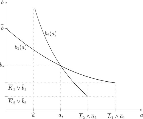These arguments, together with the additional assumptions that the inequalities ${\overline{a}}_1\wedge {\overline{L}}_1\ge {\overline{a}}_2\wedge {\overline{L}}_2$ and ${\overline{K}}_1\vee {\overline{b}}_1\ge {\overline{K}}_2\vee {\overline{b}}_2$ hold, imply that the expression ${\overline{K}}_1\vee {\overline{b}}_1<b_1(0+)\equiv \hat{b}<\mathrm{\infty }\equiv b_2(\hat{a})$ holds too. Moreover, the same arguments and assumptions directly yield that there exists exactly one intersection point with the coordinates $a_{\ast }$ and $b_{\ast }$ of the curves associated with the functions $b_1(a)$ and $b_2(a)$ on the interval $a\in (\hat{a},{\overline{a}}_2\wedge {\overline{L}}_2)$ such that ${\overline{K}}_1\vee {\overline{b}}_1<b_1(a_{\ast })\equiv b_{\ast }\equiv b_2(a_{\ast })<\hat{b}$ holds (see Figure A1 above).

Figure A1. A computer drawing of the boundary functions $b_1(a)$ and $b_2(a)$.

More precisely, let us assume that there exists at least two intersection points $(a_{\ast },b_{\ast })$ and $(\tilde{a},\tilde{b})$ of the curves $b_1(a)$ and $b_2(a)$ such that $\hat{a}<\tilde{a}<a_{\ast }\le {\overline{L}}_2\wedge {\overline{a}}_2$ and ${\overline{K}}_1\vee {\overline{b}}_1\le \tilde{b}<b_{\ast }<\hat{b}$ [or $\hat{a}<a_{\ast }<\tilde{a}\le {\overline{L}}_2\wedge {\overline{a}}_2$ and ${\overline{K}}_1\vee {\overline{b}}_1\le b_{\ast }<\tilde{b}<\hat{b}$] as well as $b_2(a)>b_1(a)$, for $a\in (\tilde{a},a_{\ast })$ [or $a\in (a_{\ast },\tilde{a})$]. Observe that, by virtue of assumptions made above and according to the implicit function theorem, it follows from the representations in (A3(A3) $\begin{array}{r}{\mathrm{\Phi }}_j^{\prime }(a)=\frac{1-{\alpha }_j}{a^{{\alpha }_{3-j}-1}}(\frac{{\gamma }_1\delta +\lambda }{(\lambda +\delta )\delta }-\frac{{\alpha }_{3-j}}{\delta })+\frac{{\alpha }_j{L}_1}{a^{{\alpha }_{3-j}}}(\frac{{\gamma }_1}{\lambda +r}-\frac{{\alpha }_{3-j}}{r})\end{array}$(A3) ) and (A4(A4) $\begin{array}{r}{\mathrm{\Psi }}_j^{\prime }(b)=\frac{1-{\alpha }_j}{b^{{\alpha }_{3-j}-1}}(\frac{{\beta }_2\delta +\varkappa }{(\varkappa +\delta )\delta }-\frac{{\alpha }_{3-j}}{\delta })+\frac{{\alpha }_j{K}_2}{b^{{\alpha }_{3-j}}}(\frac{{\beta }_2}{\varkappa +r}-\frac{{\alpha }_{3-j}}{r})\end{array}$(A4) ) that the expressions: (A10) $\begin{array}{r}{b}_j^{\prime }(a)=\frac{{\mathrm{\Phi }}_j^{\prime }(a)}{{\mathrm{\Psi }}_j^{\prime }(b)}<0\mathrm{for}j=1,2\end{array}$(A10) hold, for $a\in (\tilde{a},a_{\ast })$ and $b\in (\tilde{b},b_{\ast })$, from where it directly follows that the inequality: (A11) $\begin{array}{r}\frac{b_2^{\prime }(a)}{b_1^{\prime }(a)}>1\end{array}$(A11) is satisfied, for all $a\in (\tilde{a},a_{\ast })$. Since the derivatives $b_j^{\prime }(a)$, for j = 1, 2, from (A10(A10) $\begin{array}{r}{b}_j^{\prime }(a)=\frac{{\mathrm{\Phi }}_j^{\prime }(a)}{{\mathrm{\Psi }}_j^{\prime }(b)}<0\mathrm{for}j=1,2\end{array}$(A10) ) are continuous functions on $(\tilde{a},a_{\ast })$, we may conclude that there exists an open interval $(\tilde{a}-\epsilon ,\tilde{a}+\epsilon )$, for some relatively small $\epsilon >0$, such that the inequality $b_2^{\prime }(a)>b_1^{\prime }(a)$ holds, so that the inequality $b_2(a)>b_1(a)$ should hold, for $a\in (\tilde{a}-\epsilon ,\tilde{a}+\epsilon )$, too. However, the latter fact contradicts the assumption that the equality $b_1(\tilde{a})=b_2(\tilde{a})$ holds, which means that the curves $b_1(a)$ and $b_2(a)$ may have only one intersection point, and thus, it completes the proof of the claim.

References

- E.J. Baurdoux and A.E. Kyprianou, Further calculations for Israeli options, Stochastics 76 (2004), pp. 549–569.
- E.J. Baurdoux and A.E. Kyprianou, The McKean stochastic game driven by a spectrally negative Lévy process, Electron. J. Probab. 8 (2008), pp. 173–197.
- E.J. Baurdoux and A.E. Kyprianou, The Shepp-Shiryaev stochastic game driven by a spectrally negative Lévy process, Theory Probab. Appl. 53 (2009), pp. 481–499.
- E.J. Baurdoux, A.E. Kyprianou, and J.C. Pardo, The Gapeev-Kühn stochastic game driven by a spectrally positive Lévy process, Stoch. Process. Their. Appl. 121 (2011), pp. 1266–1289.
- E. Bayraktar and M. Sirbu, Stochastic Perron's method and verification without smoothness using viscosity comparison: Obstacle problems and Dynkin games, Proc. Am. Math. Soc. 142 (2014), pp. 1399–1412.
- M. Beibel and H.R. Lerche, A new look at warrant pricing and related optimal stopping problems, Stat. Sin. 7 (1997), pp. 93–108.
- A. Bensoussan and A. Friedman, Non-linear variational inequalities and differential games with stopping times, J. Funct. Anal. 16 (1974), pp. 305–352.
- A. Bensoussan and A. Friedman, Nonzero-sum stochastic differential games with stopping times and free-boundary problems, Trans. Amer. Math. Soc. 231 (1977), pp. 275–327.
- J.M. Bismut, Sur un problème de Dynkin, Zeitschrift Für Wahrscheinlichtskeitstheorie Und Gverwandte Gebiete 39 (1977), pp. 31–53.
- A.N. Borodin and P. Salminen, Handbook of Brownian Motion, 2nd ed., Birkhäuser, Basel, 2002.
- J. Cvitanić and I. Karatzas, Backward stochastic differential equations with reflection and Dynkin games, Ann. Probab. 24 (1996), pp. 2024–2056.
- J. Detemple, American-Style Derivatives: Valuation and Computation, Chapman and Hall/CRC, Boca Raton, 2006.
- P. Dupuis and H. Wang, Optimal stopping with random intervention times, Adv. Appl. Probab. 34 (2002), pp. 141–157.
- E.B. Dynkin, Game variant of a problem on optimal stopping, Sov. Math., Dokl. 10 (1969), pp. 270–274.
- E. Ekström and G. Peskir, Optimal stopping games for Markov processes, SIAM J. Control Optim.47 (2008), pp. 684–702.
- E. Ekström and S. Villeneuve, On the value of optimal stopping games, Ann. Appl. Probab. 16 (2006), pp. 1576–1596.
- N. El-Karoui and S. Hamadène, BSDEs and risk-sensitive control, zero-sum and nonzero-sum game problems of stochastic functional differential equations, Stoch. Process. Their. Appl. 107 (2003), pp. 145–169.
- A. Friedman, Stochastic games and variational inequalities, Arch. Ration. Mech. Anal. 51 (1973), pp. 321–346.
- P.V. Gapeev, The spread option optimal stopping game, in Exotic Option Pricing and Advanced Levy Models, A. Kyprianou, W. Schoutens, and P. Wilmott, eds., Wiley, Chichester, 2005, pp. 293–305.
- P.V. Gapeev, Perpetual double strangle options optimal stopping games, Submitted (2021), p. 20.
- P.V. Gapeev, Discounted optimal stopping problems in continuous hidden Markov models, Stochastics: An Int. J. Probab. Stochastic Processes 94 (2022), pp. 335–364.
- P.V. Gapeev, Optimal stopping zero-sum games in continuous hidden Markov models, submitted (2023), p 35.
- P.V. Gapeev and C. Kühn, Perpetual convertible bonds in jump-diffusion models, Stat. Dec. 23 (2005), pp. 15–31.
- P.V. Gapeev and H.R. Lerche, On the structure of discounted optimal stopping problems for one-dimensional diffusions, Stochastics: Int. J. Probab. Stochastic Processes 83 (2011), pp. 537–554.
- X. Guo and J. Liu, Stopping at the maximum of geometric Brownian motion when signals are received, J. Appl. Probab. 42 (2005), pp. 826–838.
- S. Hamadène and J.P. Lepeltier, Backward equations, stochastic control and zero-sum stochastic dierential games, Stochastics Stochastic Rep. 54 (1995), pp. 221–231.
- S. Hamadène and J.P. Lepeltier, Zero-sum stochastic dierential games and backward equations, Syst. Control Lett. 24 (1995), pp. 259–263.
- S. Hamadène, J.P. Lepeltier, and S. Peng, BSDE with continuous coefficients and application to Markovian non-zero sum stochastic dierential games, in Pitman Research Notes in Mathematics Series, 364, N. El-Karoui and L. Mazliak, eds., Longman, Harlow 1997, pp. 115–128.
- D.G. Hobson, The shape of the value function under Poisson optimal stopping, Stoch. Process. Their. Appl. 133 (2021), pp. 229–246.
- J. Kallsen and C. Kühn, Pricing derivatives of American and game type in incomplete markets, Finance Stochastics 8 (2004), pp. 261–284.
- I. Karatzas and S.E. Shreve, Brownian Motion and Stochastic Calculus, 2nd ed., Springer, New York, 1991.
- I. Karatzas and H. Wang, Connections between bounded-variation control and Dynkin games, in Optimal Control and Partial Differential Equations 363 (Volume in Honour of Alain Bensoussan), J.L. Menaldi et al., eds., IOS Press, Amsterdam, 2001, pp. 363–373.
- Y. Kifer, Game options, Finance Stochastics 4 (2000), pp. 443–463.
- N.V. Krylov, Control of Markov processes and W-spaces, Izvestija 5 (1971), pp. 233–266.
- C. Kühn and A.E. Kyprianou, Callable puts as composite exotic options, Math. Finance 17 (2007), pp. 487–502.
- A.E. Kyprianou, Some calculations for Israeli options, Finance Stochastics 8 (2004), pp. 73–86.
- J. Lempa and H. Saarinen, A zero-sum Poisson stopping game with asymmetric signal rates, Appl. Math. Optim. 87, 35 (2023), pp. 1–32.
- J.P. Lepeltier and M.A. Mainguenau, Le jeu de Dynkin en théorie générale sans l'hypothèse de Mokobodski, Stochastics 13 (1984), pp. 25–44.
- G. Liang and H. Sun, Dynkin games with Poisson random intervention times, SIAM J. Control Optim.57 (2019), pp. 2962–2991.
- H.R. Lerche and D. Stich, A harmonic function approach to Nash-equilibria of Kifer-type stopping games, Stat. Risk Model. 30 (2013), pp. 169–180.
- R.S. Liptser and A.N. Shiryaev, Statistics of Random Processes I, 2nd ed., Springer, Berlin, 2001.
- J. Neveu, Discrete-Parameter Martingales, North-Holland, Amsterdam, 1975.
- B. Øksendal, Stochastic Differential Equations. An Introduction with Applications, 4th ed., Springer, Berlin, 1998.
- G. Peskir, A change-of-variable formula with local time on curves, J. Theor. Probab. 18 (2005), pp. 499–535.
- G. Peskir, Optimal stopping games and Nash equilibrium, Theory Probab. Appl. 53 (2008), pp. 558–571.
- G. Peskir, A duality principle for the Legendre transform, J. Convex. Anal.19 (2012), pp. 609–630.
- G. Peskir and A.N. Shiryaev, Optimal Stopping and Free-Boundary Problems, Birkhäuser, Basel, 2006.
- S. Qiu, American strangle options, Research Rep. Probability and Statistics Group, School of Mathematics, The University of Manchester, 22 2014.
- L.C.G. Rogers and O. Zane, A simple model of liquidity effects, in Advances in Finance and Stochastics (Essays in Honour of Dieter Sondermann), K. Sandmann and P. Schönbucher, eds., Springer, Berlin, 2000, pp. 161–176.
- D. Revuz and M. Yor, Continuous Martingales and Brownian Motion, 3rd ed., Springer, Berlin, 2005.
- A.N. Shiryaev, Optimal Stopping Rules, Springer, Berlin, 1978.
- A.N. Shiryaev, Essentials of Stochastic Finance, World Scientific, Singapore, 1999.
- L. Stettner, On a general zero-sum stochastic game with optimal stopping, Probab. Math. Stat. 3 (1982), pp. 103–112.