Response characteristics and maneuverability of a small twin screw displacement hull vessel in seas

Abstract

This paper presents the response characteristics and maneuverability of a small twin screw displacement hull vessel quantified through a series of full-scale trials conducted in different environmental conditions. The 20-m test vessel is instrumented with actuator, environmental, and motion sensors. Several different maneuvers are performed at different speeds, including steady maneuvers with constant control input and transient maneuvers with varied control input to quantify and characterize the response of small vessels to aid in automatic controller and simulation development. Straight-line runs are performed in both forward and reverse over the entire operating range of the test vessel to investigate the relationship between throttle position, RPM, and surge velocity. Turning maneuvers are conducted over the achievable rudder deflection range to quantify the vessels turning radius and the relationships with surge, sway, and rotational speed. Other maneuvers include stationary rotation with the engines operating in opposite gears, and transient tests when the vessel is rapidly accelerated and decelerated. These actuator tests not only quantify the response of the actuators, but also set guidelines for the minimum dwell times that should be observed when shifting gears. These data found using a comprehensive sensor suite provide valuable benchmarks for several maneuvers that can be used for simulation validation and the actuator response information provides valuable set points and performance characteristics/limitations that should be considered in control development. The data from these tests were repeatable from run to run and thus, with sufficient instruments, at sea maneuvers can be used to collect a comprehensive set of data that can expand on data collected in tow tests.

Key words:

• Maneuverability
• response
• surface vessel
• small vessel
• full-scale trials
• sensor package

INTRODUCTION

Small displacement hull ships (< 75 m) are commonly used by the military for many applications; some of which include mine counter-measure operations (where small vessels are used in missions to locate and disable mines) (Committee for mine warfare assessment 2001), cargo and troop transfer/deployment (Keith 2004), cargo and personnel transfer between vessels (More and Hanlon 2003), and reconnaissance missions (Committee for mine warfare assessment 2001). Special Forces teams rely on small vessels for many missions to transport small numbers of soldiers at high speed while trying to avoid detection (Committee for mine warfare assessment 2001). Smaller underactuated vessels (< 75 m) are also being increasingly used for research applications (NOAA 2007; FAU 2007; WHOI 2007) because advances in technology have yielded smaller research instruments and robots such as Remotely Operated Vehicles (ROVs) and Autonomous Underwater Vehicles (AUVs) that are deployable from these vessels. Commercial and recreational fishing vessels are also often less than 75 m and equipped with twin propellers and rudders. These are just a few of the many uses of smaller displacement hull vessels, all of which currently require a skilled captain to maneuver and hold the vessel near a fixed location.

Automatic maneuvering and station keeping capabilities will greatly enhance the value of small vessels for military and civilian applications through increased operational capabilities and reduced manning by eliminating anchoring and reducing reliance on manual control. Logistical operations benefit from having small vessels autonomously station keep relative to larger vessels. Deploying and recovering an AUV, ROV, sensor, fish trap, and other items require a vessel to hold geographic position for a period of time, ranging from minutes to days, and automatically controlling position yields easier to operate, more productive vessels requiring less crew. Special Forces can use autonomous control to quickly maneuver through minefields undetected while performing coastal clandestine operations by following a prespecified path based on information from mine reconnaissance systems. Unfortunately, developing automatic maneuvering and station keeping capabilities are not easy tasks because most small vessels are underactuated, that is they are unable to directly control all three horizontal degrees of freedom independently. As a result, thrust forces and steering forces cannot be generated in the necessary degrees of freedom. Also, for a maneuvering and station keeping system to be immediately useful and widely applicable, it must be able to directly integrate into existing vessels without significant retrofits and modifications, such as the addition of new thrusters. Thus, to help understand and quantify the feasibility and limitations of maneuvering and station keeping systems for small vessels, at sea measurements are needed. These measurements provide data to quantify the response of the vessel to the environment and actuator states (rudder angle and propeller RPM), as well as relationships between the states of internal systems and vessel states. For example, when traveling forward, the propellers rotation cannot be instantaneously reversed. Instead, time must be spent in neutral until the rotation of the engines and propellers decrease before safe shifting is possible.

Measurement of the real vessel response is also valuable for developing accurate small vessel simulations that are used in maneuvering and position control systems development (ITTC 2002). Simulations are used to tune and analyze controllers because tests can be quickly completed that would otherwise require long and costly full-scale trials (Esteban et al. 2001). However, while these simulations are convenient, they must be reasonably accurate to yield relevant results. Tuning and validation of simulations is typically accomplished by using vessel maneuvering data obtained from scaled model tests and full-scale trials (Barr 1993; Plante et al. 1998; Ayaz et al. 2002; ITTC 2002; Kobayashi et al. 2003). Extensive data sets of scaled model tests exist that include tow tank and sea keeping results (Ridgely-Nevitt 1967). These results are typically included in models and used for validation. However, data sets from model basin tests are limited to a restricted set of maneuvers and actuator states. Also, because scale models do not include internal systems, such as engines and gear boxes, measurements also do not relate the vessel response to the states of the on board systems. At sea maneuvers are needed to extend the model basin tests because full-scale trials conducted with a comprehensive sensor suite provide a wider set of data to help develop a more complete system model that includes the actuator response and the complex interaction between vessel state and actuator response—an important step in developing safe and effective control systems, while avoiding extensive full-scale trials.

While at sea maneuvering data is important, little work has been done to establish full-scale maneuvering benchmark data. The 23rd ITTC Maneuvering Committee Report states that there is little full-scale maneuvering data available, and that trials with the tanker Esso Osaka are the only instrumented experiments widely cited (Kobayashi et al. 2003). No other comprehensive source of ship and model tests for any ship of more “modern” hull form could be identified by this committee (Kobayashi et al. 2003). No benchmark data was found by the author on the maneuverability of small displacement hull vessels.

In this paper, the maneuverability of a small displacement hull vessel is quantified through at sea maneuvers that yielded a benchmark data set. Data is simultaneously collected from wind and current sensors, a comprehensive suite of inertial sensors, and onboard instruments. A series of maneuvers were conducted that include transiting in a straight line with both propellers at the same RPM, transiting in circles with the rudder at a fixed angle, and maneuvers utilizing different actuator states. In Section 2, the test vessel is introduced, the environmental, actuator, and navigational sensors are described, and the data acquisition system is presented; in Section 3, navigational data fusion is presented; in Section 4, the response of the vessel during full-scale trials are examined; and in Section 5, conclusions are drawn and suggestions are made for future work.

TEST VESSEL AND INSTRUMENTATION

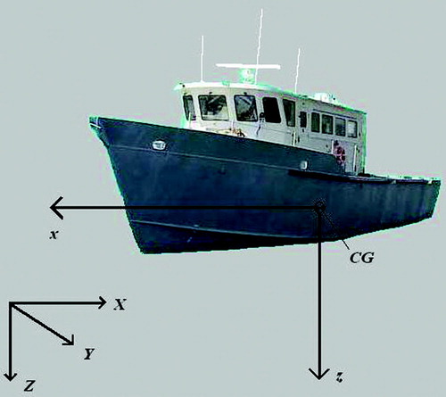
Control input states, environmental conditions, inertial, and geodetic measurements are simultaneously collected at high sample rates while the test vessel, the R/V Stephan, performed a series of maneuvers in open ocean trials. The R/V Stephan (Figure 1) is a 20-m research vessel operated by Florida Atlantic University. It has a 5.77 m beam, a 1.52 m draft, and twin rudders. It is powered by twin Detroit Diesel engines (model 7082–7399), each with 450 shaft horse power at 2300 RPM, yielding a cruising speed of about 6 m/s (FAU 2007). Engine RPM ranges between 575 and 2500 RPM, which corresponds to a propeller RPM between 230 and 1,000.

Figure 1 A picture of the 20-m R/V Stephan used for full-scale trials with the body- and earth-fixed coordinate systems attached.

Collecting at sea maneuvering data requires a comprehensive sensor suite and data acquisition system to obtain quality data and minimize errors that arise from integrated sensor bias, signal contamination, and other sensor inaccuracies. Also, measurements need to be corrected for the effects of temporally and spatially varying wind, current, and waves (Kobayashi et al. 2003). For this reason, great care is taken to select and integrate the sensor systems. The complete measurement system (Figure 2 and Figure 3) consists of three categories of sensors (actuator sensors, inertial motion sensors, and environmental sensors), a data acquisition system, and a near-real time data display and storage system. The measured actuations (control inputs) are the throttle position, RPM of the two propellers, and the angle common to both rudders. The boat's inertial motion measurements are linear accelerations, linear and angular velocities, and geodetic position and angular orientation, all in three dimensions. The environmental conditions recorded are air and water velocities relative to the boat. For all trials, additional wind measurements were recorded at a nearby meteorological station.

Figure 2 Diagram showing the flow of analog and digital streams between the data acquisition system and sensors. The blocks represent major components and lines show how they are connected.

Figure 3 A picture of the portable data acquisition system used to record data during full-scale trials. This data acquisition system has several inputs and outputs in the back of the pelican box housing, and also includes an IMU, tilt sensor, compass, NMEA multiplexer, analog filtering and power board, and a PC104 stack.

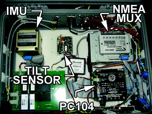
The data acquisition system itself is portable and self-contained (Figure 3). It has six external analog inputs, seven asynchronous RS232 input/output ports. Three of the RS232 ports connect directly to the computer and four are NMEA 0183 inputs, which are combined using a NMEA multiplexer and fed into one of the four asynchronous RS232 communication ports on the PC104 computer. Two NMEA 0183 inputs are used by the Differential Global Positioning System (DGPS), and one by the wind sensor. One RS232 input port is used to collect data from the Acoustic Doppler Current Profiler (ADCP). Two of the external analog inputs are used for DC current signals from the tachometers. The remaining three external analog inputs are used for DC voltage signals. One DC input is a differential voltage from the rudder, which is isolated by an isolated operational amplifier and the remaining two measure DC voltages are from throttle position sensors. Internal to the data acquisition system are a tilt sensor, a compass, and an Inertial Measurement Unit (IMU). The analog outputs from the tilt sensor and IMU are fed into a PC104 stack (the outputs from the IMU are first low pass filtered). Analog signals are converted to digital approximations using a 16 bit A/D converter. The PC104 also has a video output so data can be viewed in near-real time.

Control measurements

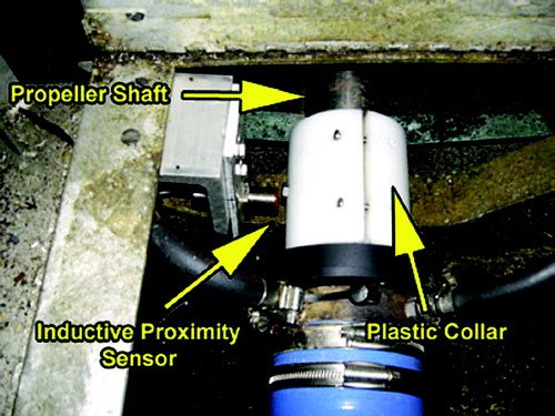
To measure throttle positions, potentiometers, which are linear over the entire actuation range, are placed on the two-engine room throttle and gear control units. The analog voltage outputs from these potentiometers are fed into two-analog voltage inputs of the data acquisition system. To measure propeller RPM, each of the two propeller shafts is outfitted with a plastic collar and two ferrous metallic inserts on opposing sides of the shaft collar. Inductive proximity sensors detect the passing of the inserts as the shaft rotates (Figure 4). Binary outputs from these sensors are read by stand-alone tachometers, which have internal 8-Hz hardware update rates. DC current output from the tachometers is sent to the data acquisition system.

Figure 4 The RPM sensor system attached to the propeller shaft of the R/V Stephan during trials. The pickup, which is attached to the bracket, senses the bolts in the shaft collar as the shaft rotates, and sends a binary signal to the rate sensor.

The rudder angle is measured using a potentiometer attached to the steering mechanism, directly above the rudder axel. The differential voltage produced by the potentiometer is directly input into the data acquisition system. Propeller RPM, throttle position, and rudder angle measurements are sampled at 100 Hz with a resolution of 0.05 RPM, 0.03°, and 0.03°, respectively.

Environmental measurements

Wind and current measurements are taken during full-scale trials to help quantify environmental disturbances and to provide the necessary data to calculate the velocity of the vessel through the water during maneuvers. The motion of the air relative to the boat is measured using an ultrasonic anemometer, which is mounted on the mast of the boat, 11 m above the water line. Three orthogonal wind velocity measurements (aligned with the axes of the vessel) are sent to the data acquisition system at 10 Hz, in a NMEA serial string. The wind sensor has a published resolution of 0.01 m/s and an accuracy of ± 0.05 m/s (R. M. Young Company 2001).

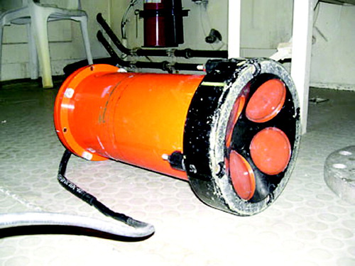
The relative velocity of the water past the vessel is measured using a through hull mounted 1200 kHz ADCP (Figure 5). The ADCP outputs a serial string at 1 Hz, which is processed using a stand-alone computer, and then sent to the data acquisition system via a serial string at 1 Hz. The latter sting contains the 3D relative water velocity with a published accuracy of 0.02 m/s for a vertical resolution of 2 m (Teledyne 2006). Mean water velocities for 2-m vertical bins were recorded at mean depths of 3 and 5 m, well below the hull boundary layer and disturbed water.

Figure 5 A 1200-kHz ADCP used to record the relative water velocity below the test vessel during trials. This ADCP was installed in a through hull fitting at approximately midship.

Inertial and geodetic measurements

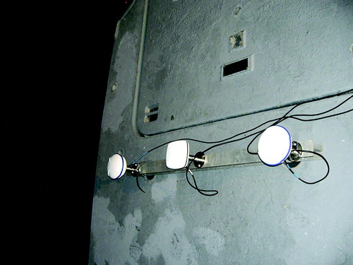
The two dimensional horizontal geodetic planer position and velocity along with true heading and rate of heading change of the R/V Stephan are measured using a dual antenna DGPS compass (Figure 6). This DGPS system outputs NMEA 0183 serial string messages that contain heading data at 10 Hz and position data at 5 Hz. This vector sensor DGPS system has a published heading accuracy of 0.1° 95% of the time with 0.1° resolution and submeter accuracy for positions 95% of the time with 0.02-m resolution (CSI Wireless Inc 2005).

Figure 6 The dual GPS antennas and DGPS beacon antenna affixed to the R/V Stephan during trials. During measurements, the antennas were mounted on the back deck of the vessel.

Linear acceleration and angular velocities of the boat are measured with a set of three orthogonal accelerometers and gyros mounted inside the data acquisition box (Figure 3). These measurements have an output angular velocity and linear acceleration noise of less than 0.01° per second and 0.018 m/s², respectively, and bias variance of less than 0.2° per second and 0.012 m/s² per year, respectively (BEI 1998). The IMU produces DC voltage signals that are low pass filtered and sampled at 100 Hz.

The tilt of the boat is measured using a two-axis tilt sensor, which is also internal to the data acquisition system (Figure 3). It has a range of ± 60° along both axes, a repeatability of ± 0.1°, and a mechanical crosstalk error of 0.025° per degree tilt (Fredericks Company 2007). This tilt sensor outputs an analog voltage that is sampled at 100 Hz.

A second measure of heading is provided by a magnetic compass internal to the data acquisition system (Figure 3) and it is used to align the sensors contained in the data acquisition box with the sensors mounted on the vessel. This compass outputs serial data at 16 Hz and measures heading with an accuracy of 1.0° RMS when tilted and has a resolution of 0.1° (PNI 2002).

INERTIAL AND GEODETIC DATA FUSION

Inertial and geodetic measurements are made using multiple complementary sensors that measure different quantities and have different error dynamics, mounting locations, alignments, and frames of reference. These measured values are therefore transferred to a common coordinate system prior to fusion. Two distinct reference systems are used—an earth-fixed coordinate system, ℑ _E , and a body-fixed coordinate system, ℑ _B , (Figure 1). Capitalized variables indicate terms in ℑ _E and lower case variables indicate terms in ℑ _B . ℑ _E is fixed to the earth and follows the NED configuration with X pointing toward the north, Y pointing toward the east, and Z pointing down. ℑ _B is fixed to the center of gravity of the boat with the x-direction pointing toward the bow, the y-direction pointing starboard, and the z-direction pointing toward the bottom of the boat (Fossen 1994). Complementary measurements are then fused to yield signals that are both accurate and precise. This is done using complementary filters that combine state measurements and their derivatives to minimize the effects of bias and drift while increasing the effective sensor resolution (Mudge and Lueck 1994; Driscoll et al. 2000; Kim et al. 2003; Conroy et al. 2005).

The complementary filter is implemented by combining a low frequency signal with its higher frequency derivatives according to a method suggested by Mudge and Lueck (1993),

where T _c is the cut off period, ξ is a state variable, (•) _L denotes a low-frequency signal, (•) _H denotes a high-frequency signal, and (•) _C is the combined measurement. These combined measurements are then low pass filtered, removing bias and noise from the measurement and creating the fused signal denoted by (•) _F .

Rotational measurements

Angular velocities are measured directly from rate gyros that are fixed to the vessel and they are denoted as ω _g = [p _g q _g r _g ] ^T , where p _g , q _g , and r _g are the angular velocities measured by the gyro about the x−, y−, and z-axes, respectively. The velocity measurements do not constitute a vector space, and therefore, their integration is meaningless. Thus, to integrate the angular velocities, angular rates must first be converted into Euler rates, = [ ] ^T . The Euler rates are calculated from gyro measurements using the following transformation matrix (Etkin 1972):

where (•) _F indicates that a fused estimate of the Euler angles estimated from the previous time step is used. This delay has a negligible effect on the measurement accuracy since the motions of the vessel are much slower than the 100-Hz update rate of the data acquisition system.

The fused Euler angle estimates that define how the vessel is oriented are calculated using the Euler rates (2) and low frequency Euler angle estimates. The tilt sensor and the compass provide measurements of the low-frequency vessel orientation. These measurements are transformed into low-frequency estimates of the Euler angles using,

where (•) _L is a low-frequency estimate, ε _x and ε _y are the tilt angles along the x- and y- axes measured by the tilt sensor, and ψ_compass is the heading measured by the compass. The low-frequency Euler angle estimates are combined with their high-frequency derivatives using Equation (1) and then low pass filtered to find the fused estimates of the Euler angles.

Linear motion signals

The sensor and measurement system used during the trials provide high-quality estimates of the vessel's acceleration in three degrees of freedom (DOF) and the horizontal planar estimates of the vessel's velocity and position. Linear acceleration measurements along the x-, y-, and z- axes [udot], [vdot], and [wdot]) are made in ℑ _B and are converted to ℑ _E using the fused Euler angles and then gravitational acceleration is removed,

where (•) _F is dropped from the fused Euler angle estimates used in this matrix for brevity. The linear acceleration in ℑ _E is the high-frequency derivatives of the velocity used when estimating the velocity of the boat.

Low-frequency linear velocity measurements from the GPS are fused with acceleration estimates from the IMU to yield enhanced velocity estimates in ℑ _E , [[Xdot] _F = [Xdot] _F [Ydot] _F Ż _F ] ^T , using the complementary filter (1), in the same manner as fusing Euler angle estimates. This filtered linear velocity is the high-frequency position derivative used when estimating the position of the boat.

In the same manner, the low-frequency position measurements from the GPS are fused with the high-frequency fused velocity estimates to yield enhanced position estimates, X _F = [X _F Y _F Z _F ] ^T .

AT SEA MANUEVERS

Three full-scale trials were conducted at sea using the R/V Stephan to establish benchmark maneuvering data for a small twin screw displacement hull vessel. This maneuvering data quantifies the performance and limitations of such vessels to aid in controller development as well as simulation development and validation. During these trials, the boat's response to control inputs is measured along with prevailing environmental conditions. These trials were performed off the Southeast coast of Florida in water ranging from 7 to 50 m in depth in minimal sea state. The average environmental conditions are presented in Table 1. The wind data, in this table, is from a Navy meteorological station approximately 2 km from the site where the maneuvers were conducted for the first two trials and averaged over the entire experiment. An onboard wind sensor was used in the third trial and data were averaged over each maneuver. The current (water velocity) data in this table, for the third trial, is calculated using the vessel mounted ADCP measurements by subtracting the vessel motions, converting the data into ℑ _E , and averaging over each maneuver. The significant wave heights are based on observations made during the trials. The wind speeds, current speeds, and significant wave heights range from 2.72 to 6.39 m/s, 0.10 to 0.41 m/s, and 0.2 to 0.35 m, respectively.

Table 1 Summary of average environmental conditions measured during trials. Wind speed and direction are recorded at an adjacent shore-based meteorological station for the first two trials, and measured using an onboard wind sensor for the third sea trial. The current speed and direction were measured using a ship mounted ADCP, and the significant wave height is based on observations

Sea trial #	1	2	3
Mean wind speed (m/s)	6.39	2.72	5.64
Mean wind direction (°)	135	104	144
Mean current speed (m/s)	0.41∗	0.12∗	0.10
Mean current direction (°)	NR	NR	43
Significant wave height (m)	0.35	0.2	0.2
The abbreviation “NR” means that measurements were Not Recorded and

The first two trials were conducted to test and tune the sensor and data acquisition systems as well as to develop sets of maneuvers for a comprehensive experiment plan. During these test trials, useful data were collected for a limited set of maneuvers and they are therefore used in this analysis. An opportunity presented itself to measure the performance of the vessel with a dirty hull for the first sea trial and the remaining two trials were performed with a clean bottom. For the first sea trial, the vessel's hull had not been cleaned in several months and had approximately 30 mm of biological growth. Thus, the vessel response, subject to greater skin friction due to this growth, was able to be quantified under a limited set of maneuvers. During the third trial, a comprehensive set of maneuvers were performed with each maneuver being repeated several times to verify that the results are repeatable. Variations in the measurements result because the response of the vessel is not only a function of actuator settings, but also a function of the varying environmental conditions and biological growth on the vessel. These variations will influence the repeatability of the data as the environmental disturbances are different from run to run and biological growth is not the same for all the trials.

The maneuverability and actuator response of the test vessel is quantified using constant input control states (throttle and steering) and varied input control states. Constant input maneuvers are used to quantify the open loop, steady state, linear and angular response of the vessel. Control settings are rapidly varied to determine the acceleration of the vessel, actuator response, and maximum rate at which the control states can be safely changed. Actuator response tests are included to determine the maximum rudder actuation rate, inherent delays when shifting gears, and the minimum RPM of the engines.

Results from the trials are presented relative to water velocity measured by the ADCP, when available, to minimize current effects. The wind measurements, in the legends, are presented with respect to the water velocity, when available, to put the ship in a pseudo no current situation by subtracting the water velocity from other velocity measurements.

Response to constant input control states

Twin screw displacement hull vessels are only able to independently control their surge and yaw motions. Because of this limitation, there are three general methods for maneuvering. These are controlling the surge motion alone (when moving in a straight line with only stabilizing rudder inputs), controlling the surge and yaw motions together (when turning), and controlling the yaw motion alone (when rotating at a fixed location). A vessel can only maneuver to or maintain a desired position utilizing these three maneuvers. While surge and yaw are the primary motions of the vessel, there are also sway motions caused by environmental effects and secondary effects from maneuvering such as centripetal acceleration.

In the first data set examined, the throttle and steering are held at different fixed positions to determine the steady-state response of the vessel. These maneuvers include (1) straight-line runs with both engines thrusting in the same direction where the steering is only used to hold course, (2) turning maneuvers with the rudder at a fixed angle and with the engines both in forward at similar RPM, and (3) rotational maneuvers with the rudder at zero degree, one engine in forward, and one engine in reverse, at similar RPM.

The Southeast Florida shoreline (where tests were conducted) runs predominately north–south and near-shore currents are predominately along shore, with magnitudes ranging between 0 and 1 m/s. Thus, two runs in opposite directions are performed for most of the straight-line tests to obtain a differential measure of the effect of current and wind. For example, straight-line tests were performed heading north. Immediately following, identical runs were performed heading south. For turning and rotational maneuvers, at least one complete rotation was performed for each propeller RPM and rudder angle combination. This ensures that all turning maneuvers include environmental forces from all directions. The velocities presented for the turning maneuvers are thus averaged over an integer number of complete rotation for each set of control inputs.

Straight-line maneuvers

For typical operations, twin screw vessels move in a straight line by operating engines at or near the same RPM while maintaining a ruder angle near zero degrees. The rudder is used only minimally to stabilize the vessel and maintain the desired heading. To quantify the straight-line response of the vessel and determine the relationship between propeller RPM, throttle position, and velocity, several test runs were conducted while maintaining a fixed heading while traveling in both the forward and backward (astern) directions. Data also provide a measure of the effect of environmental conditions on a vessel and the effect of a dirty hull. The tests were conducted in minimal seas with light to medium wind. The direction the wind is blowing toward and the current flowing from is referenced to the average heading of the vessel for a particular set of tests to show the effect of environmental conditions on the vessel's performance. For each RPM investigated, the throttle was held constant for approximately 5 min and the velocity is averaged over the last 3 min when the vessel reached a steady speed.

Forward direction. Straight-line runs were carried out while traveling forward with both engines operating at similar forward RPM and minimal rudder deflection. In each straight-line segment, the vessel was operated over the range of RPM, between 230 and 900, which represents the full range of propeller rotational velocity (Figure 7). Five straight-line segments were performed with the hull clean. Three line segment maneuvers were performed during trial 3 while ADCP measurements were simultaneously recorded and these data sets were normalized to still waters. The remaining two line segment maneuvers (with no current data) were not normalized with the ADCP data and were performed on a different day during trial 2. The clean hull segments that were not normalized with the ADCP followed the same trend as the clean hull normalized data and exhibit a nearly constant offset of 0.24 m/s between measurements made at similar RPM settings while transiting in opposite directions. The offset is likely due to the presence of a small current parallel to the vessel path of approximately 0.12 m/s flowing toward the north and variations in the offset are due to changes in the current and wind. Thus, to normalize the data, the 0.12 m/s current is removed from these two data sets (Figure 8). All five clean hull-normalized data sets exhibit strong repeatability with a standard deviation with respect to the curve fit line of 0.075 m/s, which is primarily due to wind, waves, and variations in boat handling.

Figure 7 Surge velocity measured relative to the earth for straight-line runs at different propeller RPM and minimal rudder deflection where (+) indicates data from a vessel with a dirty hull. The legend gives the mean wind speed during each run and the mean direction the wind is blowing toward with respect to the heading of the vessel. The solid line is third-order curve fit to clean hull data, and the dashed line is a third-order curve fit to dirty hull data.

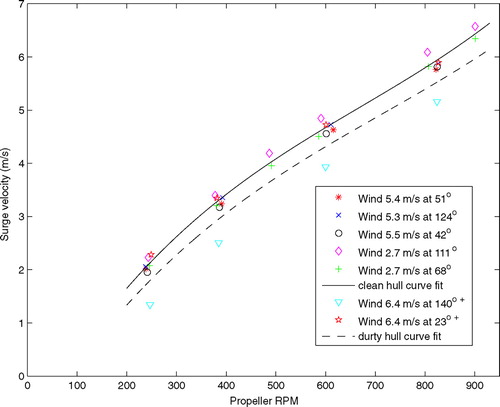
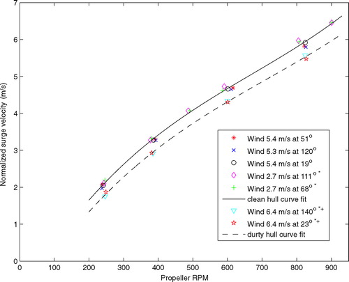
Figure 8 Surge velocity measured relative to the water for forward straight-line runs at different propeller RPM and minimal rudder deflection where a (∗) indicates that current data is not available and thus is normalized with respect to the estimated current and (+) indicates data from a vessel with a dirty hull. The legend gives the mean wind speed during each run and the mean direction the wind is blowing toward with respect to the heading of the vessel. The solid line is curve fit to clean hull data, and the dashed line is curve fit to dirty hull data.

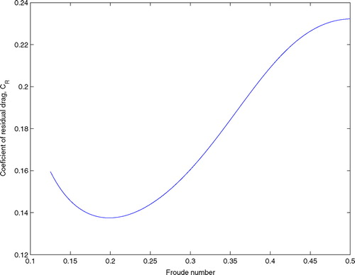
The measurements from the clean hull data are used to calculate the residual drag coefficient for the vessel. This is done by assuming that skin friction, propeller thrust, and residual drag produce the dominant forces when the vessel is moving in a straight line at a constant speed. The force due to residual drag is isolated by removing the skin drag and propeller forces using an analytic formula for skin drag separately published by Prandtl and von Karman (Lewis 1998) and a propeller thrust model (Fossen 1994), respectively. The residual drag is then converted to its nondimensional coefficient form using C _R = − 2f _R /(ρ Su _rel ²), where f _R is the estimated force from residual drag, S is the wetted surface area, u _rel is the measured relative surge velocity, and ρ is the density of sea water. The residual drag coefficient is presented as a function of the Froude number (Figure 9). The shape of this curve with the local minimum near a Froude number of 0.2, inflection near 0.37, and largest value within the range at 0.5 are consistent with residual drag curves produced by Lewis (1998) using scale model tow tank tests. Thus, it is possible to use at sea maneuvers to produce similar data to tow tank tests when necessary measurements are available.

Figure 9 Residual drag coefficient derived from the clean hull straight-line runs by estimating and removing the skin drag and propeller thrust from the force balance in the body fixed x-direction, then solving for C _R .

Two straight-line maneuvers were performed while transiting in opposite directions with a dirty hull in trial 1. Again, no current measurements were recorded to normalize the data. For this set of maneuvers, there is a constant offset between measurements taken when transiting in different directions (Figure 7)—a similar feature was noted in trial 2. The mean difference between these two un-normalized dirty hull straight-line runs is 0.83 m/s, indicating that, on average, a southward 0.415 m/s water velocity component is present and thus it is used to normalize the data (Figure 8). For the dirty hull maneuvers, the average velocity is 9.4% less than of the velocity measured with a clean hull for similar RPMs. This is primarily due to the added skin drag from the biological growth. The shapes of the dirty and clean hull surge velocity curves are nearly identical. The offset between the clean and dirty curves increases slightly with propeller RPM and this is a direct result from the “dirty” propeller, which has less efficiency. Thus, the overall effect of this extreme dirty hull is, on average a 9.4% effective increase in drag and an estimated 10.6% increase in RPM is needed to achieve the same velocity.

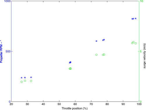
The propeller RPM and normalized forward velocities are presented with respect to the throttle position for the three straight-line maneuvers conducted during trial 3 (Figure 10) to aid in controller development where direct throttle actuation is used. There is a dead band in the throttle position between 0 and 27% of the throttles' range. The throttles must therefore be moved by at least 27% of their actuation range before the propellers begin to rotate. This is the throttle setting at which the clutch begins to engage and the throttle begins to “open” increasing the fuel flow to the engine. The data also show that the relationships forward velocity to throttle position and propeller RPM to throttle position are roughly linear once the clutch is fully engaged, at 40% of full range. Thus, unlike electric prime movers that have incremental propeller response to throttle settings, small vessels with direct drive systems do not. Instead, the propeller response to throttle settings is characterized by a dead zone (neutral), a transition state where the clutch and throttle engine cable begin to engage, and an incremental zone with a proportional response. Therefore, to develop effective control systems for small vessels and representative numerical models, these characteristics need to be included in the development.

Figure 10 The propeller RPM (∗), left ordinate and surge velocity (o), right ordinate measured during forward straight-line runs with equal RPM for two engines, and minimal rudder deflection.

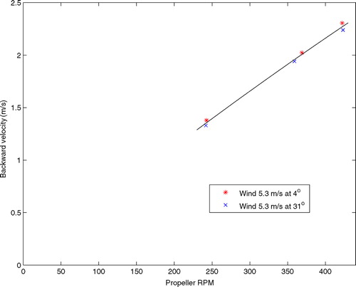
Aft direction. Two straight-line runs are also carried out during the third full-scale trial with both engines operating at a similar reverse RPM while rudder deflection is minimized (to control the heading only). Several different propeller RPM settings that represent the full reverse operating range, from 230 to 425, were investigated while traveling into the wind to help stabilize heading of the vessel (Figure 11). The maximum reverse propeller RPM is limited to 425 RPM because cavitation occurs at higher settings. The data were normalized with respect to the current and were repeatable between different segments (Figure 11). For this limited set of maneuvers, the speed of the vessel is approximately linearly proportional to the RPM, and the magnitude of the backward speed is approximately 70% of the forward speed at similar RPM. The maximum reverse speed of the test vessel before cavitation is approximately 36% of the maximum forward speed of the vessel. The overall speed reduction is caused by the added drag of the blunt stern and rudders when operating in reverse and the reduced efficiency of the propellers.

Figure 11 The backward (negative surge) velocity for reverse propeller RPM range between 230 and 425 for straight-line runs in reverse. Results are normalized and presented relative to the mean current. The legend gives the mean wind speed during the runs, and the mean direction the wind is blowing with respect to the heading of the vessel.

For the two reverse straight-line maneuvers, the propeller RPM and normalized velocities are presented as functions of throttle position to quantify the relationship between throttle position, aft velocities, and RPM (within the range where cavitation does not limit performance). Again, there exists a dead zone where the throttle must be rotated by more than 27% to engage the propellers in reverse and the throttle should not be actuated beyond 62% to avoid cavitation. This range is important for applying automatic controllers because it quantifies the range of neutral (where throttle movements are meaningless) and sets maximum limits to avoid cavitation.

Turning tests

Normally, a vessel is turned in transit by deflecting the rudders while both engines are at the same forward RPM. This creates a moment on the vessel resulting in a rotational velocity and induced secondary sway motions that are both functions of the RPM, rudder angle, and environmental forces. Therefore, to quantify the steady-state motions of the vessel when turning, both engines are placed at the same forward RPM and the rudder deflection is held constant while the boat completes at least one 360° rotation. This maneuver is repeated for incremental values of rudder deflection between −37° and 37°, the operational range of the rudder, excluding very small angles, for two different propeller RPMs. The angular velocity, side velocity, and forward velocity for each actuator combination are estimated by averaging instantaneous measurements over an integer number of complete turns. This eliminates initial transient values and averages the influence of environmental forces for each data point. The normalized magnitudes of these motions from the third trial are compared for propeller RPMs of 380 (Figure 12, Figure 13, Figure 14) and 580 (Figure 16, Figure 17, Figure 18). Rudder angles smaller than |± 9°| for a propeller RPM of 380 and |± 5°| for an RPM of 580 produced moments too small to counteract the wind moment on the vessel. Thus, the test vessel was unable to complete a full circle because it went in a straight line when the moments balanced. Therefore, only data above these set points are presented. The wind speeds, which are averaged over each series of circles, varied by 1.7 m/s between the different sets of maneuvers and these small variations did not, on average, produce a significant change in the vessel's response. The measurements were very repeatable—the variance between the individual values and the curves fit to the data (straight line for r when rudder angle < 23°), for propeller RPM of 380 (580), are 0.015 (0.024)°/s for rotational velocity, r, 0.010 (0.009) m/s for the surge velocity, u, and 0.002 (0.002) m/s for sway velocity, v. Variations seen in the different data sets are likely due to slight differences in RPM between the port and starboard propellers, asymmetry in the hull (such as a through-hull port on the starboard side where the ADCP was mounted), and local environmental variations.

Figure 12 Magnitude of rotational velocity as a function of the absolute value of the rudder angle for both engines operating at an RPM of approximately 380. Data are presented for five different runs and the legend identifies the direction the vessel is rotating, clockwise (starboard turning rudder) and counterclockwise (port turning rudder), along with mean wind speed for each set of circular maneuvers.

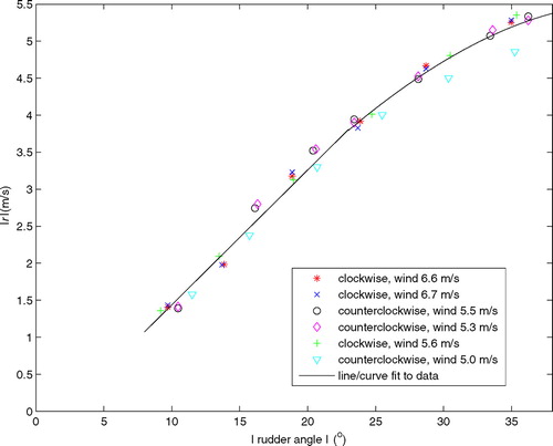
Figure 13 Surge velocity as a function of the absolute value of the rudder angle for both engines operating at an RPM of approximately 380. Data are presented for five different runs and the legend identifies the direction the vessel is rotating, clockwise (starboard turning rudder) and counterclockwise (port turning rudder), along with mean wind speed for each set of circular maneuvers and the dashed line is the forward velocity when moving in a straight line.

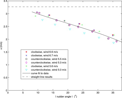
Figure 14 Magnitude of the sway velocity as a function of the absolute value of the rudder angle for both engines operating at an RPM of approximately 380. Data are presented for five different runs and the legend identifies the direction the vessel is rotating, clockwise (starboard turning rudder) and counterclockwise (port turning rudder), along with mean wind speed for each set of circular maneuvers.

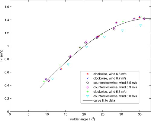
Figure 15 The sway velocity squared (v ²) of which sway drag is a function and the product of surge velocity and rotation rate (ur) of which centripetal acceleration is a function, for an RPM of 380, as a function of rudder angle.

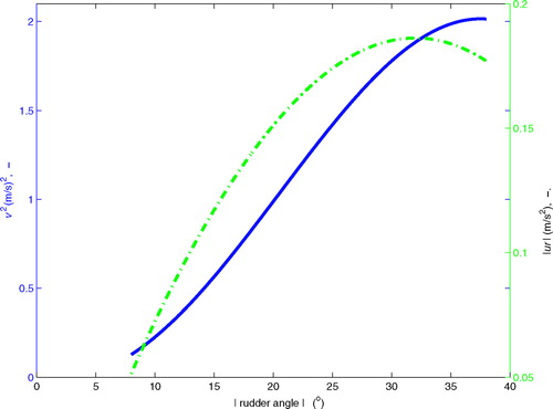
Figure 16 Magnitude of rotational velocity as a function of the absolute value of the rudder angle for both engines operating at an RPM of approximately 580. Data are presented for five different runs and the legend identifies the direction the vessel is rotating, clockwise (starboard turning rudder) and counterclockwise (port turning rudder), along with mean wind speed for each set of circular maneuvers.

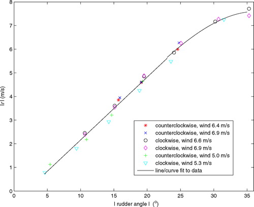
Figure 17 Surge velocity as a function of the absolute value of the rudder angle for both engines operating at an RPM of approximately 580. Data are presented for five different runs and the legend identifies the direction the vessel is rotating, clockwise (starboard turning rudder) and counterclockwise (port turning rudder), along with mean wind speed for each set of circular maneuvers and the dashed line is the forward velocity when moving in a straight line.

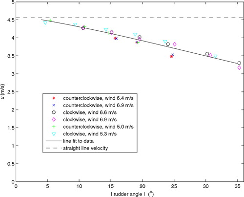
Figure 18 Magnitude of the sway velocity as a function of the absolute value of the rudder angle for both engines operating at an RPM of approximately 380. Data are presented for five different runs and the legend identifies the direction the vessel is rotating, clockwise (starboard turning rudder) and counterclockwise (port turning rudder), along with mean wind speed for each set of circular maneuvers.

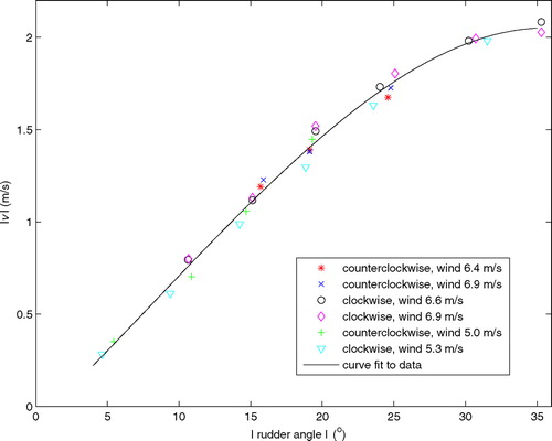
When a rudder is deflected during transit, the primary intent is to change heading while maintaining forward speed. When the rudders are deflected, the angular rate, r, increases with rudder deflection (Figure 12 and Figure 16), the forward velocity, u, is reduced (Figure 13 and Figure 17), and the radial velocity (sway), v, is generated (Figure 14 and Figure 18). At rudder angles less than 25°, the rate of turn is linearly proportional to the rudder angle, which is consistent with conventional rudder models (Choi et al. 2004), where lateral force is nearly proportional to deflection angle. At greater deflections, separation of the flow over the rudder occurs and the rate of change of r with respect to the rudder angle decreases. The maximum turn rate achieved was 5.5 (7.5)° per second at 380 (580) RPM, which is equivalent to completing circles with approximate radii of 26 (29) m in 68 (47) s. This shows that as speed increases, the rotation rate and turning radius also increase for identical rudder angles.

Turning the rudder not only creates a moment, it also induces drag and deflects propeller wash that, in turn reduces the surge velocity (Figure 13). The surge velocity decreases linearly and this is consistent with the approximate linear increase in the rudder drag in conventional rudder models (Choi et al. 2004). The maximum surge velocity reduction was 1.4 (1.3) m/s from the straight-line velocities at 380 (580) RPM, which is a 42 (29)% reduction. As the rudder angle decreases, the surge velocity converges toward the values of the steady straight-line runs (Section 4.1.1), demonstrating consistency between the two different sets of maneuvers.

The sway velocity produced during a steady turn is primarily a balance of sway drag, f(v ²) to the lateral centripetal acceleration f(ur) and rudder force, f(α), where α is the rudder angle. As previously discussed, the lift from the rudder increases roughly linearly with increasing α, while separation begins at around 27°. The centripetal acceleration is also roughly linear for small angle and then the slope rapidly decreases with the maximum value of centripetal acceleration at a rudder angle of 30°. For this reason, the square of the sway velocity is approximately linear for small rudder angles with the slope rapidly decreasing with centripetal acceleration and after stall occurs at around 27° (Figure 15).

Rotation about a fixed location

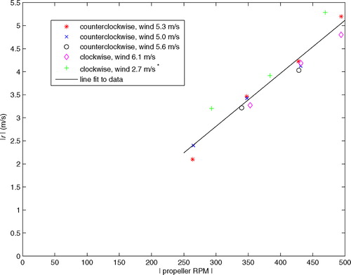
To turn a twin screw vessel about a fixed location, one engine is typically placed in forward and one in reverse, creating a net moment on the vessel while the forward and astern thrust balance. This is commonly used for docking, maintaining a fixed location, or maneuvering in a restricted area. To investigate the response of the test vessel for such a maneuver, the engines of the vessel are placed at the same RPM with one propeller operating in forward, one in reverse, and the rudder angle is held at zero degree. The angular velocity (Figure 19) is estimated by averaging data over an integer multiple of complete rotations where the RPM is limited to values less than 500 because cavitation begins when the astern thrusting propeller RPM is greater. Maneuvers are conducted at several different RPM during trials two and three. Turning data at RPM below 260 RPM were not presented because moments generated are insufficient to counter the wind moment. The data show that angular velocity is linearly proportional to RPM and the variance of the data is 0.06° per second about a linear fit. The maximum steady-state angular velocity achieved is approximately 5° per second, which is near the maximum steady-state angular velocity achieved while transiting forward at 380 RPM and turning with the rudder (Figure 12). At 500 RPM, the vessel can complete a rotation in about 70 s without encountering cavitation. During these maneuvers, secondary surge and sway velocities were also created. Because the propellers were operated at the same RPM, the decreased efficiency of the propeller operating in reverse, compared to the propeller operating in forward, created a force imbalance that propelled the vessel forward at speeds from 0.3 to 1.0 m/s and sideways at speeds from 0.4 to 0.9 m/s. By matching the forward and astern thrust instead of matching RPM, these linear motions could be reduced.

Figure 19 Angular velocity and average propeller RPM measured for trials 2 and 3, with one engine in forward, one engine in reverse, and a rudder angle of approximately 0°. The (∗) indicates that the wind speed is not measured on the vessel, but is instead measured at a nearby meteorological station.

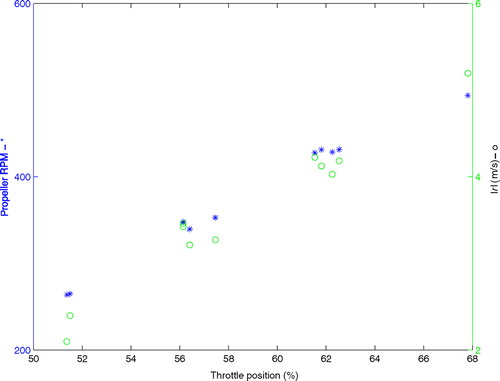
Because of the cavitation limit on the propeller RPM, only a limited number of data points were recorded that relate the throttle position to propeller RPM and the turn rate. However, in the range of data presented, the clutch was fully engaged and the propeller RPM and throttle position are linearly proportional (Figure 20). Thus, the RPM and rotational velocities are also nearly linearly proportional. The lowest throttle position is 51%, which yields a turn rate of about 2.2° per second and the largest throttle position is 68%, which yields a turn rate of about 5.3° per second.

Figure 20 Propeller RPM and rotational velocity for different propeller RPM and minimal rudder deflection, with each propeller having equal RPM, but thrusting in opposite directions.

Response to varied input control states

In this section, the transient response of the test vessel is quantified for maximum surge acceleration and deceleration. Unlike the steady maneuvers where the vessel's response is dominated by hydrodynamic effects, the transient response is also a function of the vessel's inertia, the dynamics of actuator systems, and the rate of change of control states such as throttle position (determined by the captain or control system). Thus, the transient response of the vessel needs to be quantified to validate numerical models that simulate unsteady maneuvers as well as to determine realistic relationships between control state actuation rates, propeller response, and vessel response. To do this, the transient response of the vessel is examined when the boat is accelerated at the maximum allowable rate that will not damage the ship, based on the captain's judgment, from rest to near maximum forward speed without engaging the turbocharger. Using the turbochargers is avoided since they require up to 10 s to engage, even when the throttles are at their maximum deflection because the engines must first reach a critical RPM. When disengaging the turbochargers, the RPM can be decreased quickly. However, it is important to decrease the RPM slowly to allow adequate cooling. For these reasons, the turbocharger should not be used for short-term maneuvering, such as station keeping, and it should be reserved for longer runs. After a steady speed is reached, the throttle position is rapidly reduced until the engines are in neutral, and measurements are taken until the vessel comes to rest.

Forward acceleration

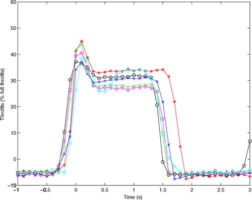
To investigate the response to maximum acceleration, the test vessel is accelerated from a state of drift until the vessel reaches its maximum speed without engaging the turbochargers. Three different runs were performed and during each run, the captain rapidly increased the throttle to 50%, briefly dwelled at 50% for about 0.75 s, and then rapidly increased the throttle up to 70%–100% (Figure 21). By averaging the three runs, and not exceeding any instantaneous maximum throttle position, the throttle position can be safely changed from 0 to 75% in 2 s. The resulting propeller RPM increases by about 100 RPM/s for propeller RPM less than 450, even when the vessel's speed is less than 1 m/s. During this test, the response of the propeller is delayed with respect to the throttle setting by as much as 1 s (Figure 22). The throttle positions are not maintained at their maximum position during this test because the turbochargers will engage if both throttles are held above 75% for more than approximately 10 s.

Figure 21 (a) Time series of the throttle position (b) and propeller RPM, when the vessel is accelerated from a state of drift until the vessel reaches its maximum speed without engaging the turbochargers. The solid lines are a filtered average of the measured data.

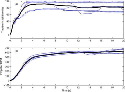
Figure 22 Time series of the throttle position and propeller RPM during the initial stages of acceleration. The horizontal difference between two lines is the lag between throttle actuation and propeller response.

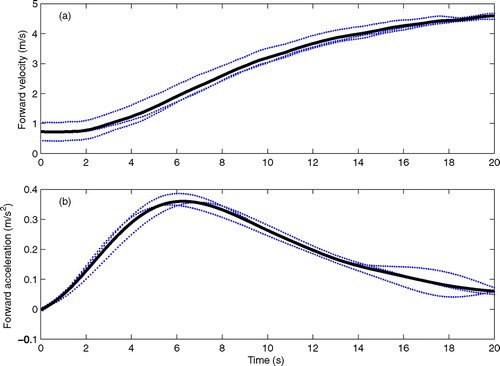
When the throttle is rapidly changed from 0 to maximum setting, the vessel accelerates at up to 0.35 m/s², with maximum acceleration occurring approximately 6 s after throttles are initially moved, Figure 23. The vessel can reach 4 m/s in approximately 15 s, which is 60% of the full speed of the vessel.

Figure 23 Time series of forward speed relative to water (a) and forward acceleration (b), when the vessel is accelerated from a state of drift until the vessel reaches its maximum speed without engaging the turbochargers. The solid lines are a filtered average of the measured data.

Forward deceleration

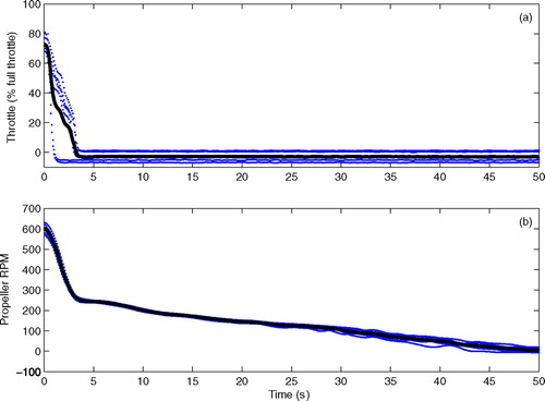
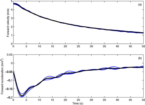
The deceleration of the vessel when moving in a straight line and shifting the engines into neutral is investigated during trial 3 to quantify the maximum actuation rate of the throttles and the corresponding vessel response. During these maneuvers, the boat is initially moving at near maximum forward speed (while turbochargers are disengaged), and then the throttle positions are rapidly decreased to shift the engines into neutral as quickly as the captain feels is possible without risking damage to the engines. The boat is then allowed to slow until it comes to rest. The throttles were rapidly reduced from 75% to neutral, and in one case this was done in 1 s (Figure 24). In each case, the throttle actuation time was less than 3 s. The average time for the throttles to decrease to neutral (a throttle setting of 27%) was 1.5 s. The propeller responds, decreasing the RPM to below minimum in gear value of 230 RPM, in 3.5 seconds. The 2-s delay between the time the throttle is in neutral (at t = 1.5 s) and steady propeller RPM result, because the clutch disengages before the momentum of the shaft and the propeller allows the RPM to decrease to their minimum in gear value. After the clutch disengages and the rotation momentum is damped out, the propellers begin to rotate in the free stream, driven by the water flowing past the vessel. The vessel reached its maximum deceleration rate of 0.19 m/s² at 2.5 s, which is approximately 50% of the maximum acceleration measured in the acceleration maneuver. In the first 20 s, the forward velocity decreased by 50%, and in the next 30 s, the forward velocity decreased to 25% of the initial forward velocity at t = 0. In the same 50 s, the vessel travels 118 m, approximately 6 boat lengths. This provides a base distance from a specified location in which a vessel must begin to slow if it is to stop at a location with no overshoot or reverse thrust.

Figure 24 Time series of the throttle position (a) and propeller RPM (b), when the vessel is decelerated from maximum forward velocity without operating the turbochargers to a drift. The solid lines are a filtered average of the measured data.

Actuator dynamics

Actuators cannot respond instantaneously and their dynamic response is often a limiting factor when controlling a vessel, either manually or automatically. Functional limitations of actuation are not always strictly defined because they are not physical limitations. Instead, they are often in the form of operational procedures adopted to avoid excessive strain and wear on the actuators. One such procedure is the dwell time between shifting gears. This time delay differs between operators, but general guidelines for automatic control can be determined by analyzing the dwell time experienced in manual operation by an experienced operator. The following three tests are added to more clearly define the actuator dynamics. These tests quantify maximum rudder deflection and turn rate, maximum rate of change of RPM, dwell time between shifting gears, and minimum functional RPM.

Figure 25 Time series of the throttle position and propeller RPM during the initial stages of deceleration. The dashed blue line indicates the throttle setting where the clutch disengages and the minimum in gear propeller RPM. The horizontal difference between two lines is the lag between throttle actuation and propeller response.

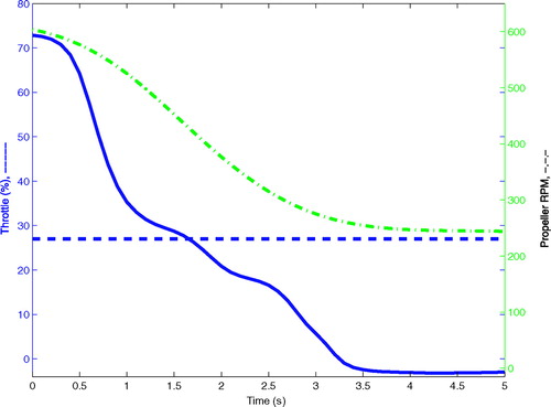
Figure 26 Time series of the forward velocity relative to the water (a) and forward acceleration (b), when the vessel is decelerated from maximum forward velocity without operating the turbochargers to a drift. The solid lines are a filtered average of the measured data.

Rudder dynamics

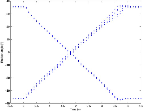
The steering system is investigated as the rudder is deflected from one extreme position to the other by rotating the steering wheel at a rate that exceeds the hydraulic system capacity. This process is repeated nine times during trial 3 to estimate the maximum rotation rate of the rudder. The rudder has a range of ± 37° and can be rotated throughout its full range of motion in 3.7 s, Figure 27. The rudder deflection is nearly linear over this range with a constant maximum angular velocity of 20° per second. It cannot be rotated faster than this without physical modification.

Figure 27 Time series of the rudder position when it is deflected at a maximum rate from one maximum deflection angle to the other.

Engine response

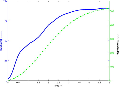
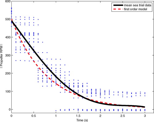
In this section, the maximum rate of change of throttle position and corresponding propeller RPM is quantified for a vessel that is nearly stationary. The knowledge of rapid engine response is needed for developing control systems for precise yet high-powered maneuvering, such as when docking, or attempting to maintain an exact location. The propeller response is investigated by quickly actuating the throttles from neutral to maximum thrust in either forward or reverse. During this test, the throttle is then reduced back to neutral 6 s after initial actuation. In this time, the vessel gains a speed of up to 1.7 m/s. The process is repeated a total of 17 times, and the data from these tests is curve fit. Data from this test show that the propeller can reach 400 RPM in about 1 s (Figure 28). The magnitude of the propeller RPM then increased, albeit at a slower rate, and nearly reached 500 at 3 s. Thus, the propeller can achieve nearly 55% of full scale within 2 s. After 2 s, the rate of increase is much less. When the propeller RPM is quickly reduced from approximately 500, the minimum in-gear RPM is reached within 1 s. The propeller RPM approaches 0 within 2 s of the initial throttle movement. This more rapid reduction in RPM, as compared with maneuvers in the section labeled forward deceleration, results because the rotational friction on the propellers is higher at lower vessel speeds. Thus, a short burst of propulsion can be achieved in a window spanning less than 4 s. This response can be approximated using the following first-order system:

Figure 28 Time series of the propeller RPM when quickly actuating the throttle from neutral to full throttle while the boat is nearly stationary. The data points are from 17 different tests, and the solid line is a curve fit to this data.

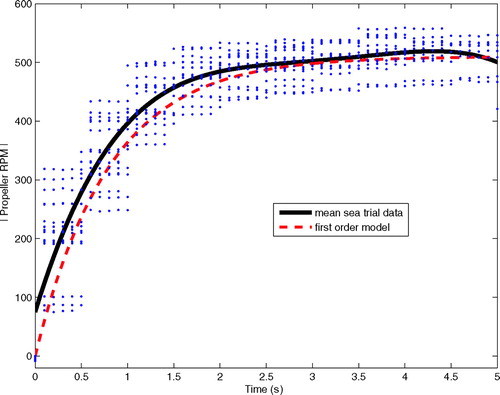
The response of this system to a step input (Figure 28 and Figure 29) is a good estimate of the engine response, for both increasing and decreasing RPM when the vessel is nearly stationary.

Figure 29 Time series of the propeller RPM when quickly actuating the throttle from near full throttle to neutral while the vessel is nearly stationary. The data points are from 17 different tests, and the solid line is curve fit to this data.

Engine shifting dynamics

When shifting gears, it is important to dwell at neutral before shifting again. This allows the propeller RPM to slow so that the strain generated when the propellers and shafts are forced to switch direction is minimized or at least structurally tolerable. The dwell time is not only important when shifting between forward and reverse, but also when shifting in and out of gear in the same direction of rotation. Quantifying this dwell time and the minimum functional RPM is important because automatic controllers may specify an RPM that is less than the minimum RPM of the engine, or they may specify a rapid change in actuator values between gears. In either case, the physical limitations and practical considerations must be included in numerical models and the controller. To quantify the minimum dwell time, the operator repeatedly shifted between forward and reverse. While operating near idle speed, a propeller RPM of 230 (Figure 30a), there should be at least a 2.5-s dwell time in neutral when shifting between forward to reverse. Because of the added shaft, propeller, and engine momentum this time should be increased to 4 s when operating at a higher initial RPM as indicated in Figure 31a. This dwell time allows for the propeller cease rotation (Figure 30b and Figure 31b) before the clutch engages and begins to rotate the propeller in the opposite direction. A similar test is conducted for shifting between forward and neutral. This test shows that there should be at least a 2.0-s dwell time when shifting into neutral and then into the same gear (Figure 32) and a 1.5-s dwell time when shifting from neutral (Figure 33) into and then out of gear.

Figure 30 Time series of the throttle position (a) and propeller RPM (b) when switching from forward to reverse as quickly as the Captain feels is safe when the in-gear RPM is near the minimum RPM of the vessel and the motion of the vessel was minimal. The gears engage when the throttle is at approximately 27% of its actuation range.

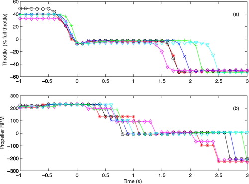
Figure 31 Time series of the throttle position (a) and propeller RPM (b) when switching from forward to reverse as quickly as the Captain feels is safe when the in-gear RPM was near the maximum RPM of the vessel, the engine is not in turbo, and the motion of the vessel is minimal. The gears engage when the throttle is at approximately 27% of its actuation range.

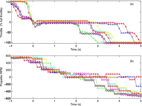
Figure 32 Time series of throttle position when switching from forward to neutral, and then back into forward, as quickly as the Captain feels is safe when the in-gear RPM is near the minimum RPM of the vessel and the motion of the vessel is minimal. The gears engage when the throttle is at approximately 27% of its actuation range.

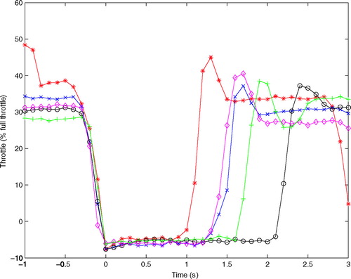
Figure 33 Time series of throttle position when switching from neutral to forward, and then back into neutral, as quickly as the Captain feels is safe when the in-gear RPM is near the minimum RPM of the vessel and the motion of the vessel is minimal. The gears engage when the throttle is at approximately 27% of its actuation range.

CONCLUSIONS

A comprehensive data acquisition package has been developed to measure navigational data, actuator states, and environmental conditions. The navigational sensors include a dual antenna GPS compass, IMU, and tilt sensors to record the motion of the vessel in six degrees of freedom. Measurements are combined and filtered at high sample rates to yield high-quality estimates of linear position, velocity, and acceleration, and angular orientation and velocity in three dimensions. Simultaneously the throttle position, propeller RPM, and rudder angle are also recorded along with wind and current measurements.

Three full-scale trials are conducted using a 20-m test vessel equipped with the aforementioned sensor system. Through these trials, the maneuvering performance and actuator responses of the vessel are quantified. Steady-state maneuver data for straight-line runs, turning maneuver using the rudder, and rotational maneuver with one engine in forward, and one engine in reverse, are analyzed with the data showing good repeatability. The standard deviation from a curve fit to the data range from 0.075 to 0.1 m/s for the forward (sway) velocity, 0.04 to 0.04 m/s for the sway velocity, and 0.12 to 0.25° per second for the rotation rates. Straight-line tests demonstrate that forward velocity is approximately a linear function of RPM, and that the maximum velocity of the vessel is 6.5 m/s, at a propeller RPM of 900. As well, a dirty hull with approximately 0.03 m of biological growth reduces the forward speed by approximately 9.4%. Rotational maneuvers and straight-line runs in reverse showed that cavitation limits the thrust that can be produced. When both engines are in reverse, cavitation begins at a propeller RPM of 425, and when one engine is in forward and one in reverse, cavitation begins at 500 RPM. Rapid throttle actuation tests were used to quantify the acceleration of the vessel and response of the engines and rudders. The engine response to throttle input can be represented with a first-order model that converges to the steady-state RPM. The propellers can reach an RPM of 500 in 5 s and a forward speed of 4 m/s can be reached in 16 s. The maximum rotational rate of the rudder is nearly constant at 20° per second. These actuator tests not only quantify the response of the actuators, but also set guidelines for the minimum dwell times that should be observed when shifting gears.

These data found using a comprehensive sensor suite and data acquisition system allow for analysis of the complete system response. This not only includes drag and maneuvering data typically found using tow tank tests, but also actuator system data, which is dependent on state. This allows for important and limiting phenomena such as cavitation to be evaluated, which is not easily evaluated using either propeller models tow tank testing alone. These data provide valuable benchmarks for several maneuvers that can be used for simulation validation and the actuator response information provides valuable set points and performance characteristics/limitations that should be considered in control development.

ACKNOWLEDGMENTS

The authors would like to thank the office of naval research, code 33, program manager Kelly Cooper for partially funding this work under grants N00014–06-1–0461 and N00014–03-1–0211. J. H. VanZwieten would like to thank the College of Engineering and Computer Science at Florida Atlantic University and the Ocean Engineering department for a teaching assistantship.

Notes

(∗) indicates that the current speeds are estimated from the difference in the forward velocity from the straight-line runs in opposite directions. The wind and current directions are the directions that the wind and current are flowing toward.

REFERENCES

- Ayaz , Z , Vassalos , D , Spyrou , K J and Matsuda , A . . Towards a unified 6 DOF maneuvering model in random seas . Proceedings of the 6th International Workshop on Stability and Operational Safety of Ships, Webb Institute . October 13–16 , New York. Paper no. 2, Workshop 3
- Barr , R . 1993 . A review and comparison of ship maneuvering simulation methods . Transactions of SNAME , Vol. 101 : 609 – 635 .
- BEI Technologies, Inc. 1998 . BEI MotionPak—Multi-axis inertial sensing system, Data Sheet , Concord, CA : BEI Technologies, Inc .
- Choi , B , Park , H , Kim , H and Lee , S H . . An experimental evaluation on the performance of high lifting rudder under coanda effect . Proceedings of the 9th Symposium on Practical Design of Ships and Other Floating Structures . September 12–17 , Luebeck-Travemuede, Germany.
- Committee for Mine Warfare Assessment . 2001 . Naval mine warfare: operational and technical challenges for naval forces , 133 – 158 . Washington, DC : National Academic Press .
- Conroy , J , Samuel , P and Pines , D . . Development of an MAV control and navigation system. AIAA-2005–7065 . AIAA 5th Aviation, Technology, Integration, and Operations Conference . September 26–29 2005 , Arlington, VA.
- CSI Wireless Inc. 2005 . CSI wireless vector sensor and vector sensor pro reference manual , 15 Calgary, , Canada : CSI Wireless Inc .
- Driscoll , F R , Lueck , R G and Nahon , M . 2000 . The motion of a deep-sea remotely operated vehicle system. Part 1: motion observations . Ocean Engineering , 27 : 29 – 56 .
- Esteban , S , de Andres , B , de la Cruz , J M and Giron-Sierra , J M . . Smoothing fast ferry vertical motions: a simulation environment for the control analysis . EUROSIM 2001 Congress shaping future with simulation . June 26–29 2001 , Delft, Netherlands.
- Etkin , B . 1972 . Dynamics of atmospheric flight , New York : Wiley .
- c1999–2007 . Florida Atlantic University: Department of Ocean Engineering , Boca Raton, FL : Florida Atlantic University . http://www.oe.fau.edu/research_vessels/stephan.html Available from, accessed on 11 July, 2007
- Fossen , T I . 1994 . Guidance and control of ocean vehicles , 38 Chichester, UK : Wiley .
- Fredericks Company . 2007 . Huntingdon Valley, PA : The Fredericks Company . http://www.frederickscom.com/products/pdf/0729–1720.pdf Available from, accessed on 11 July, 2007
- International Towing Tank Conference . . ITTC recommended procedures and guidelines . Proceedings of the 23rd International Towing Tank Conference . SNAME, Doc. No. 7.5-02-06-03
- Keith , ME . 2004 . A model for studying world war II-era LCMs in the archaeological record [master's thesis] , Tallahassee, FL : Florida State University .
- Kim , J H , Wishart , S and Sukkarieh , S . . Real time navigation, guidance, and control of an UAV using low cost sensors . Proceedings of the International Conference of Field and Service Robotics (FSR03) . July 2003 , Yamanashi, Japan. pp. 95 – 100 .
- Kobayashi , H , Blok , J J , Barr , R , Kim , Y S and Nowicki , J . 2003 . Specialist Committee on Esso Osaka: Final Report and Recommendations to the 23rd ITTC Vol. 2 , 581 – 743 .
- Lewis , E V . 1988 . Principles of naval architecture . The Society of Naval Architects and Marine Engineers , 2 : 7 – 10 . 26; 3:198, 248
- More , C W and Hanlon , E . 2002 . Sea basing: operational independence for a new century . United States Naval Institute Proceedings, , 129 ( 1 ) : 80 – 85 .
- Mudge , T D and Lueck , R G . 1994 . Digital signal processing to enhance oceanographic observations . Journal of Atmospheric and Oceanic Technology , 11 : 825 – 836 .
- NOAA Ship Rude . 2007 . Norfolk, VA : National Oceanographic and Atmospheric Administration . http://www.moc.noaa.gov/ru/index.htm Available from
- Plante , M , Toxopeus , S , Blok , J and Keuning , A . . Hydrodynamic maneuvering aspects of planing craft . Proceedings from the International Symposium and Workshop on Forces Acting on a Maneuvering Vessel . September , Val de Reuil, France. pp. 147 – 155 .
- PNI Corporation . 2002 . TCM2 electronic compass module user's manual , Santa Rosa, CA : PNI Corporation .
- Young R.M. Company . 2001 . Model 81000 ultrasonic anemometer manuel PN 81000–90 , Traverse City, MI : R. M. Young Company .
- Ridgely-Nevitt , C . 1967 . The resistance of a high displacement-length ratio trawler series . Transactions of the Society of Naval Architects and Marine Engineers , 75 : 51 – 78 .
- Teledyne RD Instruments . 2005 . San Diego, CA : Teledyne RD Instruments . http://rdinstruments.com/datasheets/wh_sentinel.pdf Available from
- Woods Hole Oceanographic Institute . 2007 . Woods Hole, MA : Woods Hole Oceanographic Institute . http://www.whoi.edu/marops/research_vessels/CRV/index.html Available from, accessed on 11 July, 2007