A 4 DOF simulation model developed for fuel consumption prediction of ships at sea

ABSTRACT

The study presents a new simulation model for the prediction of the fuel consumption of ships at sea. The model includes external forces and moments caused by the environment at sea, i.e. wind, waves and ocean currents, and solves the force and moment balances for the ship with four degrees-of-freedom (4 DOF), i.e. surge, drift, yaw and heel. To capture involuntary speed losses, engine limits are included in the model. By combining an existing power prediction model, a numerical standard hull and propeller series, and numerous empirical methods, the simulation model can be applied to conventional ships with very limited information available at the outset of an analysis, e.g. the main dimensions, engine rpm and propeller rpm. Additionally, a wind-assisted propulsion component is available. The current study describes the details of the 4 DOF model together with its applicability on three case studies on a ship route through the Baltic Sea with realistic weather forecasts. The main conclusions of the study show that there are considerable differences in the predicted fuel consumption when comparing simulation results based on 1 DOF and 4 DOF; the 4 DOF simulation model is recommended. It is shown that it is crucial to include the yaw moment balance and limits for the rudder angle when analysing ships with wind-assisted propulsion. Examples of involuntary speed losses and different modes of operation are compared and discussed, and potential problems with propeller backside cavitation and engine stalling when running a ship with a wind-assisted device are discussed.

KEYWORDS:

• Fuel consumption
• ship energy efficiency
• ship operation
• wind-assisted propulsion

Nomenclature
AR	=	Rudder area (m2)
AR	=	Aspect ratio (-)
AP	=	Aft perpendicular (–)
B	=	Breadth (m)
cB	=	Block coefficient (–)
cD	=	Drag coefficient (–)
cL	=	Lift coefficient (–)
CLR	=	Centre of lateral resistance (%)
cTH	=	Propeller thrust loading (–)
DOF	=	Degrees of freedom (–)
FP	=	Forward perpendicular (–)
g	=	Gravitational constant (9.81) (m/s2)
GM	=	Metacentric height (m)
K	=	Heeling moment (Nm)
KR	=	Rudder heeling moment (Nm)
KRI	=	Righting moment (Nm)
KW	=	Wind heeling moment (Nm)
KS	=	Heeling moment from sails (Nm)
KT	=	Propeller thrust coefficient (-)
Loa	=	Length over all (m)
Lpp	=	Length between perpendiculars (m)
N	=	Yaw moment (Nm)
NH	=	Yaw moment due to drift (sway) (Nm)
NR	=	Rudder yaw moment (Nm)
NS	=	Sail yaw moment (Nm)
NW	=	Yaw moment due to wind (Nm)
T	=	Propeller thrust (N)
TD	=	Draft (m)
TWA	=	True wind angle (deg)
TWS	=	True wind speed (m/s, kn)
vc	=	Speed of the current (m/s)
vhull	=	Hull speed in longitudinal direction (m/s, kn)
vSOG	=	Speed over ground (m/s, kn)
vSTW	=	Speed through water (m/s, kn)
vt	=	Transversal speed (m/s, kn)
X	=	Longitudinal force (N)
XD	=	Resistance due to drift (sway) (N)
XAW	=	Resistance due to waves (N)
XCW	=	Calm water resistance (N)
XSW	=	Resistance due to shallow water (N)
XR	=	Rudder resistance (N)
XS	=	Sail resistance (thrust) (N)
XW	=	Wind resistance (N)
xys	=	Longitudinal position of the sail force centre (m)
xyw	=	Longitudinal position of the wind force centre (m)
Y	=	Transversal force (N)
YH	=	Side force from drifting (N)
YR	=	Rudder side force (N)
YS	=	Sail side force (N)
YW	=	Side force from wind (superstructure) (N)
zys	=	Height of the sail force centre (m)
zyw	=	Height of the wind force centre (m)
β	=	Drift (sway) angle (deg)
δ	=	Rudder angle (deg)
Δ	=	Displacement (t)
ε	=	Angle of attack (wind, waves) (deg)
Φ	=	Heel angle (deg)

1. Introduction

A ship at sea encounters external forces from waves, wind and ocean currents. Traditionally performance analysis and prediction models follow the ITTC recommendations for sea trial tests (ITTC 2014) to estimate the power increase due to the environmental influences. Such an approach neglects side forces, yaw and heel moments from wind and waves, and focusses on the longitudinal forces (i.e. the added resistance). Under sea trial conditions, i.e. calm weather and only head or stern wind, the approach is feasible because the moments and side forces are virtually zero. However, during rougher weather conditions with varying angles of encounter for the wind and waves this is not the case – side forces and yaw moments will have to be compensated with a drift of the vessel and a rudder angle, which both cause more resistance. In some studies, such as in Naaijen et al. (2006) and Kramer et al. (2016), approaches which consider force and moment balances in four degrees-of-freedom (4 DOF), i.e. surge, drift (sway), heel and yaw, were introduced for ships with wind-assisted propulsion. It has not yet been investigated in detail how a 4 DOF simulation model compares with a 1 DOF simulation model with regards to the predictability of the fuel consumption.

The present study presents a new simulation model for the prediction of the fuel consumption of commercial ships at sea, solving the force and moment balance for 4 DOF. The model is based on former work and a 1 DOF simulation model presented in Tillig et al. (2018). It accounts for engine limits, differences in propeller efficiency and engine fuel consumption due to possible off-design operation. In contrary to the models presented in Naaijen et al. (2006) and Kramer et al. (2016), the new simulation model is completely based on empirical methods and numerical standard hull and propeller series. It makes it applicable to arbitrary ships with very limited input, i.e. only the main dimensions, the propeller rpm and the engine rpm are required. The present paper introduces the model and the methods used, and shows the applicability of the model in case studies using two ships, a tanker and a PCTC, on a route through the Baltic Sea. The case studies show the importance of employing 4 DOF simulations in comparison with of 1 DOF (i.e. pure added resistance). This is shown for both of the ships, with and without wind-assisted propulsion. Additionally, the effect of involuntary speed loss due to engine limits, and different modes of operation, on the fuel consumption are discussed.

1.1. Description of the upgraded generic energy systems model

A generic energy systems model has been developed and is presented in Tillig et al. (2017, 2018). It can be used to simulate and analyse the power and fuel consumption predictions for arbitrary merchant vessels under realistic operational conditions with very limited required input. The model consists of two parts, a static power prediction called ShipPOWER and a dynamic operation simulation model called ShipJOURNEY. ShipPOWER is the static part of the model which is described in Tillig et al. (2017), where different levels of prediction uncertainties are discussed and presented in detail in Tillig et al. (2018). The required minimum inputs are the principal dimensions (length, beam, draft, displacement), the design speed, the propeller arrangement and the propeller and engine rpm. Six sets of results are generated from ShipPOWER:

1. a hull form from the standard series including all missing dimensions (e.g. bulbous bow dimensions and superstructure areas),

2. the linear hydrodynamic derivatives for the dynamic force and moment balance; see Section 2,

3. a resistance and power prediction at calm water without wind,

4. a power prediction with Seas state four head waves and Beaufort four head wind,

5. a propeller design from the standard series, and

6. the engine limits.

Compared to the model used in Tillig et al. (2018) the estimation of the hydrodynamic derivatives is added based on different empirical formulas, as described in detail in Section 2. In addition, the dynamic route simulation part of the simulation model presented in Tillig et al. (2017) has in the new simulation model been completely reprogrammed in Matlab, and extended to capture 4 DOF by solving the force and moment equations for the surge, drift, yaw and heel. The dynamic part ShipJOURNEY is used for route simulations and it includes the possibility to evaluate the efficiency of wind-assisted propulsion such as Flettner rotors or sails; the latter motivated the necessity to extend the simulation model from 1 to 4 DOFs. ShipJOURNEY is dynamic for the large scale, i.e. changing the weather and operational conditions along the route are accounted for, however the ship dynamics (motions, manoeuvring, de- and acceleration) are not modelled. For each evaluation point along the route, the static solution for the ship. The added power in waves accounts for the added resistance but not added power due to other effects, e.g. propeller ventilation.

An overview of the simulation model is presented in Figure 1. The required input to ShipJOURNEY are results from ShipPOWER, information about the conditions along the route (wind, waves, water depth, water temperature, ocean current), and the operational conditions of the vessel (draft, target average speed, mode of operation). In the current version of the model, three modes of operation are available: (a) constant target speed, (b) constant journey time, and (c) constant engine power. Note that it is possible to replace the results from ShipPOWER by dimensions and model test results from actual ships if such results are available. Wind-assisted propulsion can by evaluated using the simulation model if the following information is available: means of thrust and side coefficients, sail area, and the centre of the total sail force in longitudinal and vertical directions.

Figure 1. Flowchart of the journey prediction model..

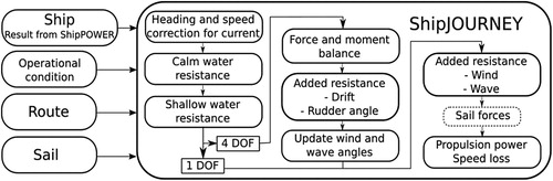
The outputs from ShipJOURNEY are the engine power, fuel consumption, ship speed, heel and drift angles at each way point along a route, as well as the total journey time and the fuel consumption. ShipJOURNEY finds the force and moment balance, handles sail forces and reefing, and ensures that the propeller working points are kept within the engine limits, i.e. it handles involuntary speed losses. With the capabilities of ShipJOURNEY and ShipPOWER, the simulation model can be applied to a wide range of situations and example cases: from ship to fleet optimisation, through retrofitting studies to route optimizations, if connected to an optimisation algorithm all with very limited information about the ship in question.

1.2. Limitations and applicability of the model

The presented model is developed to provide an accurate fuel consumption prediction with very limited required input. It can be applied to transport problems on a tactical level, i.e. for speed optimizations, routing and fleet studies, and as on-board decision making tool. Due to nature of the model (as described below) it is suitable for the prediction of the fuel consumption in changing weather during a journey, but, it cannot be used for manoeuvring or seakeeping simulations. The model is supposed to be used to estimate/analyse the energy efficiency of ships and not to simulate survival conditions, i.e. the wind speed should in general be kept below 40 kn, with the corresponding waves. The most critical component with regard to harsh weather is the added wave resistance, which was found to give good results for at least sea state 6 (waves up to 6 m), as shown in Tillig et al. (2018). In general, the methods are also valid for higher waves, but this will introduce higher uncertainties as those defined in Tillig et al. (2018). The wave spectra used for the estimation of the added wave resistance are valid for deep water waves, thus special care must be taken when simulating journey in waters with restricted water depth.

Since the model is based on empirical methods and standard hull and propeller series, it should only be used for ships that the methods and standard series are valid for, i.e. common cargo ships. Further, the model is dynamic with respect to the ship’s reaction on changes in the environmental conditions, such as changing wind speed or direction. With respect to ship motions, the model is quasi-static (no influence from inertia effects), i.e. the force and moment equations are solved for the case that the sum of all forces and moments is zero.

2. Method

2.1. Problem definition

On a ship at sea, there are outer forces and moments acting, caused by the wind and the sea. While the longitudinal parts of these forces, referred to as resistances, are accounted for by increased propeller thrust, the side forces and yaw moments must be compensated by a drift of the ship and a rudder angle. The heeling moments are compensated by the ships righting moment. Figure 2 shows the coordinate system used in the study, with the centre at FP, midships and at the keel, the x-axis pointing aft along the ships longitudinal direction, the y-axis pointing to portside and the z-axis down.

Figure 2. Coordinate system with definition of the rudder angle.

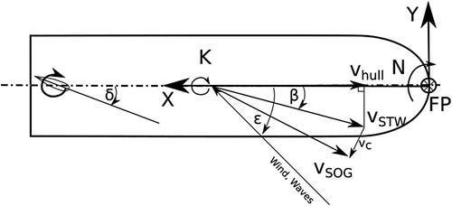
When evaluating the energy efficiency of a ship at sea, only the steady-state solution at each point of the route is of interest, which results in two special conditions when solving the equations motions: since the yaw rate is zero (the ship is not turning), the pivot point is not existing, and the sum of all forces and moments must be zero. To summarise, the system of equations in Equations (1) to (4) must be solved to find the equilibrium for one speed and one environmental condition; each force and moment is shown with the variables that it is a function of. Note that most of the terms in these equations depend on the drift angle, β. This is due to the dependency of the angle of attack of the wind and the waves on the drift angle (since the ship has to compensate for the drift).(1) $X=0=X_{CW}+X_{AW}(\beta )+X_D(\beta )+X_{SW}+X_W(\beta )+X_S(\beta \varphi )+X_R(\delta T)+T$(1) (2) $Y=0=Y_H(\beta )+Y_R(\delta T)+Y_S(\beta \varphi )+Y_W(\beta \varphi )$(2) (3) $N=0=N_H(\beta \varphi )+N_R(\delta T)+N_S(\beta \varphi )+N_W(\beta \varphi )$(3) (4) $K=0=K_S(\beta \varphi )+K_W(\beta \varphi )+K_H(\beta )+K_R(\delta T)+K_{RI}(\varphi )$(4)

2.2. Estimation of the forces and moments

In the generic ship energy systems model in Tillig et al. (2017, 2018), the total resistance of a ship at sea is composed of:

1. the calm water resistance, X_CW, estimated from two empirical methods (Tillig et al. 2017),

2. the wind resistance, X_W, estimated using curves from Blendermann (1994),

3. the added resistance due to waves, X_AW, estimated using three empirical methods (Tillig et al. 2017),

4. the added resistance due to shallow water, X_SW, estimated using the ITTC (2014) formulation for speed loss due to constrained water depth,

5. the added rudder resistance, X_R, computed using the drag coefficients from Schneekluth and Bertram (1998), and

6. the drift resistance, X_H, estimated using the lift to drag ratio derived in Kramer et al. (2016).

A detailed description and validation of the items (i) to (iv) are presented in Tillig et al. (2017). Due to the large amount of included methods and models that define the simulation model, the parts (i) to (iv) are not repeated from the detailed description in Tillig et al. (2017). Instead, this section focuses on the newly developed four DOF component of the simulation model. The expected accuracy of a fuel consumption prediction based on the available input information is discussed in Tillig et al. (2018).

In the new and upgraded version of the simulation model, thrust forces from sails, X_S, can be included by defining thrust coefficient curves over the apparent wind angle. This leads to large side forces which required a four DOF solution. However, there are several sources which cause side forces: (a) the wind resistance of the ship, Y_W, (b) the hull due to a transverse speed (drift angle), Y_H, (c) the rudder due to a rudder angle, Y_R and, (d), the sails, Y_S. In the model, the side force from the wind on the ship are estimated using the curves from Blendermann (1994), and for a wind-assisted propulsion device (e.g. a sail) it is obtained from the given side force coefficient curves for the sail.

In the following, the equations implemented in the simulation model are presented to be able to correctly consider the effect from side forces. For the static case, the hydrodynamic derivatives can be reduced to the linear parts which depend on the transversal speed (v_t). According to Inoue and Hirano (1981), the derivatives can be estimated by(5) $Y_H=\frac{1}{2}\ast \rho \ast L_{pp}\ast T\ast v_s^2\ast Y_H^{\mathrm{\prime }}$(5) (6) $Y_H^{\mathrm{\prime }}=Y_v^{\mathrm{\prime }}\ast v_t^{\mathrm{\prime }}+Y_{v_t|v_t|}^{\mathrm{\prime }}\ast v_t^{\mathrm{\prime }}|v_t^{\mathrm{\prime }}|$(6) (7) $v_t^{\mathrm{\prime }}=v_t/v_s$(7) (8) $Y_v^{\mathrm{\prime }}=-\left(\pi \ast {\displaystyle \frac{T}{L}+1.4\ast c_B\ast {\displaystyle \frac{B}{L}}}\right)$(8) (9) $Y_{v|v|}^{\mathrm{\prime }}=-\left(0.244+6.67\ast \left((1-c_B)\ast {\displaystyle \frac{T}{B}-0.05}\right)\right)$(9)

Clarke et al. (1983) give a different formulation for the derivatives and the normalisation:(10) $Y_H=\frac{1}{2}\ast \rho \ast v_s^2\ast L_{pp}^2\ast Y_H^{\mathrm{\prime }}$(10) (11) $Y_H^{\mathrm{\prime }}={\displaystyle \frac{v_t}{v_s}\ast \left(-\pi \ast {\left({\displaystyle \frac{T}{L_{pp}}}\right)}^2\ast \left(1+0.4\ast c_B\ast {\displaystyle \frac{B}{T}}\right)\right)}$(11)

A comparison between the Inoue and Hirano (1981) and Clarke et al. (1983) formulations showed that the latter resulted in slightly lower side forces. Thus, the average of the results from both formulations is used in the ShipJOURNEY model. The added resistance due to drift can be computed from the drag to lift ratio presented in Kramer et al. (2016), and it can be approximated as(12) ${\displaystyle \frac{X_H}{Y_H}=0.0004\ast {\beta }^3-0.009\ast {\beta }^2+\ast 0.0754\ast \beta -0.0015}$(12)

To capture the effects of the area ratio, i.e. the length to draft ratio for the ship, one can use the formula given in Lewis (1989) (with c_D as the drag coefficient and c_L as the lift coefficient):(12b) $c_D={\displaystyle \frac{c_L^2}{\pi \ast 2\ast (T/L)\ast 0.9}{c}_L={\displaystyle \frac{Y_H}{(\rho /2)\ast T\ast L_{pp}\ast v_S^2}{X}_H=c_D\ast {\displaystyle \frac{\rho }{2}\ast T\ast L_{pp}\ast v_S^2}}}$(12b)

It should however be noted, that the length to draft ratios of common ships are not as different as the area ratios for air foils, where formula (12b) originates from. In the case studies in this project, the expression from formula (12a) is used.

The side (YR) and drag (XR) forces generated from the rudder can be estimated according to Bertram (2000), with the rudder drag at zero degree rudder angle included in the calm water resistance:(13) $X_R=c_D\ast v_s^2\ast {\displaystyle \frac{\rho }{2}\ast A_R}$(13) (14) $Y_R=c_L\ast v_s^2\ast {\displaystyle \frac{\rho }{2}\ast A_R}$(14) (15) $c_L=2\pi \ast {\displaystyle \frac{AR\ast (AR+0.7)}{{(AR+1.7)}^2}\ast \sin \delta +\sin \delta \ast |\sin \delta |\ast \cos \delta }$(15) (16) $c_D={\displaystyle \frac{c_L^2}{\pi \ast AR}+|\sin \delta {|}^3}$(16)

Due to the propeller slipstream and the typical aftbody shape of ships, it is assumed that the inflow to the rudder follows the ships longitudinal axis. The influence of the rudder being in the slipstream of the propeller on the drag and lift can be estimated by Bertram (2000) as(17) $\mathrm{\Delta }{Y}_R=T\ast \left(1+{\displaystyle \frac{1}{\sqrt{1+c_{Th}}}}\right)\ast \sin \delta$(17) (18) $\mathrm{\Delta }{X}_R=T\ast \left(1+{\displaystyle \frac{1}{\sqrt{1+c_{Th}}}}\right)\ast (1-\cos \delta )$(18)

As shown in Figure 3, the side forces do not act in the same point, neither in longitudinal nor in vertical direction, thus causing yaw and heel moments. The vertical and longitudinal positions of the side force due to wind is estimated using the formulas developed in Blendermann (1994) while the positions for the sail forces are a direct input depending on the position and aspect ratio of the sails. An additional yaw moment is caused by the sails due to the heel angle:(19) $N_S(\varphi )=X_S\ast \sin (\varphi )\ast z_{ys}$(19)

Figure 3. Side forces and levers for the estimation of heel and yaw moments.

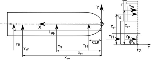
The centre of effort of the side force due to drift, CLR, can be computed from formulas for the yaw moment and the side forces due to drift. Using the method by Clarke et al. (1983), the CLR is constant at 16.2% from the FP. According to Inoue and Hirano (1981), the CLR moves forward with increasing drift angle with an additional impact from the heel angle. In the model, the average CLR from both methods due to transversal speed is used, with the impact from the heel angle applied:(20) $N_{\mathrm{Inoue}}^{\mathrm{\prime }}(\beta )=-2\ast {\displaystyle \frac{T}{L}{N}_{\mathrm{Inoue}}^{\mathrm{\prime }}(\varphi )=0.0076}$(20) (21) $N(\beta \varphi )=\frac{1}{2}\ast \rho \ast L_{pp}^2\ast T\ast v_s^2\ast (N^{\mathrm{\prime }}(\varphi )\ast \varphi +N^{\mathrm{\prime }}(\beta )\ast \sin (\beta )\ast v_{\mathrm{s}})$(21) (22) $\mathrm{CL}{\mathrm{R}}_{\mathrm{Inoue}}(\beta )={\displaystyle \frac{L_{pp}}{2}-{\displaystyle \frac{N_{\mathrm{Inoue}}(\beta )}{Y_{H-\mathrm{Inoue}}}\mathrm{\Delta }\mathrm{CL}{\mathrm{R}}_{\mathrm{Inoue}}(\varphi )=-{\displaystyle \frac{N_{\mathrm{Inoue}}(\varphi )}{Y_{H-\mathrm{Inoue}}}}}}$(22) (23) $CLR={\displaystyle \frac{0.162+CL{R}_{Inoue}(\beta )}{2}+\mathrm{\Delta }CL{R}_{Inoue}(\varphi )}$(23)

Due to the position of the coordinate centre at FP and the rudder at AP, the lever for the yaw moment of the rudder side force is equal to Lpp. The height of the centre of effort of the rudder side force and the side force due to drift (zh) is assumed to be at T/2. In summary, the yaw and heel moment is evaluated by(24) $N=0=Y_R\ast L_{pp}+Y_W\ast x_{yw}+Y_S\ast x_{ys}+N_S(\varphi )+Y_H\ast \mathrm{CLR}$(24) (25) $K=0=(Y_R+Y_H)\ast {\displaystyle \frac{T_D}{2}+Y_S\ast z_{ys}+Y_W\ast z_{yw}-GM\ast \mathrm{\Delta }\ast \sin \varphi \ast g}$(25)

2.3. Equation solving

The system of equations shown in the Equations (1) to (4) is solved using the Nelder–Mead simplex algorithm, an optimisation algorithm for nonlinear functions (Lagarias et al., 1998). This algorithm generates a simplex around the start value and approaches the local minimum of the target function by modifying this simplex. The Nelder–Mead simplex algorithm is fast and easy to use since it does not require a target function derivate. However, the algorithm is not guaranteed to find a local minimum which requires a sound first guess as the start value. The closer the first guess is to the actual minimum, the faster and robust the optimisation.

In the ShipJOURNEY part of the model, the start value is found by solving an uncoupled and simplified system of equations. Simplifications made for the start value are: (i) the influence from propeller thrust on the rudder force is neglected, (ii) the influence from heel on the yaw moment is neglected, and (iii) the equations are solved in five iterations, updating the drift angle in the estimation of the apparent wind angle and speed. A reefing of sail, if applied, is done during the definition of the start value or point, if the maximum rudder angle or maximum heel angle is exceeded. With this, the full system of equations is solved using the Nelder–Mead simplex algorithm, for each way point on the route and each ship speed of interest. The optimisation variables are: (a) the drift angle, (b) the heel angle and (c) the rudder angle, with the sum of the squares of the total side force, the total heel angle and the total yaw moment as target function. As a default, the termination tolerance is set to be 0.006 degree for the input variables (heel, drift and rudder angle) and 1000 for the target function, i.e. the sum of the squared forces and moments.

A numerical simulation with the ShipJOURNEY model with four DOF, 30 way points on a route and nine speeds takes about 320 s on an eight-core desktop PC. This is reduced to about 2 s if only one DOF is considered. The computation time increases linearly with increasing number of way points along the route and the number of speeds.

3. Results

The section presents results for performance predictions using the ShipJOURNEY model. Two ships are used in the study, one tanker and one PCTC, with the dimensions as presented in Table 1. Additional data such as non-specified dimensions, the engine curves as well as resistance and propulsion performance curves were derived using the ShipPOWER model.

Table 1. Dimensions of example ships.

	PCTC	Tanker
Loa	199.99 m	183.00 m
B	36.50 m	32.20 m
TD	9.20 m	11.00 m
Δ	36000 t	50610 t
vdesign	19 kn	15 kn

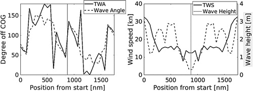
A route crossing the Baltic Sea, from Gothenburg (Sweden) through the great belt to St. Petersburg (Russia) and back, was chosen. The route is 900 nm each way. Wind and wave forecasts from the Swedish Meteorological and Hydrological Institute of December 8th were used (SMHI 2017). To better evaluate the performance of sails, the ships encountered identical weather on the way to St. Petersburg and the return trip. An impression of the route is given in Figure 4. In Figure 5 the wind speeds and wave heights are presented as encountered during the journey. During the first and the last 150 nm the ships encountered strong winds (up to 35 kn) and up to 3.2 m high waves. The vertical line in Figure 5 symbolises arrival at St. Petersburg. The water depth was derived from nautical charts, the influence from ocean current was disregarded in the study, and the water temperature was set to 15°C for the whole journey. A detailed description of the weather data can be found in Appendix 1.

Figure 4. Illustration of the route used in the study.

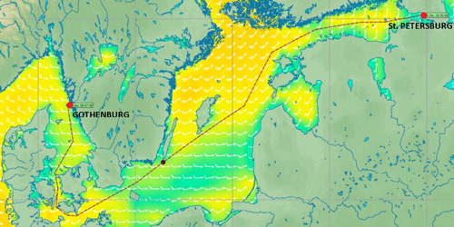
Figure 5. True wind angle (TWA), true wind speed (TWS) and waves along the route.

3.1. Comparison of 1 and 4 DOF simulations for the two ships

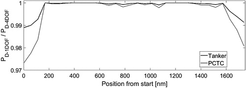
The importance of considering four degrees-of-freedom in a ship dynamic simulation model used for route simulations is shown by comparing results from one and four DOF simulations. The target speed for the tanker was set to 14 kn and to 18 kn for the PCTC. Figure 6 presents the results showing the power from the 1 DOF simulation over the power from 4 DOF simulations. For the tanker, drift and rudder resistances cause the 4 DOF power to be up to 1% higher in the regions with high wind speeds. For the PCTC, this difference is up to 3%, which is caused by the large transversal and longitudinal superstructure areas. Differences during the rest of the journey are smaller due to lower wind speeds and more head and stern winds as shown in Figure 5.

Figure 6. Comparison of the simulation results using 1 DOFand 4 DOF for the tanker and the PCTC.

3.2. Simulation of involuntary speed loss due to hard weather

High added resistance due to, e.g. wind and waves or very high added thrust from the sails can cause the required power and rpm to increase beyond the engine limits. Three scenarios can be identified: (i) the required torque exceeds the maximum torque of the engine, (ii) the required rpm exceeds the maximum rpm of the engine, and (iii) the combination of required torque and rpm is above the curve for ample air supply for the engine, i.e. the engine cannot run on such a load since at such low rpm, it cannot be supplied by enough air to produce the required torque. Each of the three scenarios will lead to an involuntary speed loss which means that the target speed cannot be reached. This effect is included in the simulation model. Severe ship motions, slamming loads or green water on deck might require a voluntary speed reduction by the crew, which is not simulated by the model.

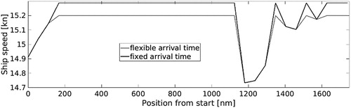
Figure 7 presents results from a performance prediction for the tanker at target speed of 15.2 kn. In the beginning of the journey at around 1200 nm from the departure port, the ship experiences involuntary speed loss. Two scenarios were simulated in the model. Firstly, the target speed was kept at 15.2 kn. During this scenario, the ship does not exceed the target speed but experiences involuntary speed loss which leads to an increase of the journey time by 30 min. The speed profile of this scenario is shown as the grey line in Figure 7. In the second scenario, the target speed is increased to achieve the journey time as defined through the average target speed, shown as the black line. This scenario requires an optimisation loop to find the required target speed to achieve the average speed despite the speed loss. The target speed during the second scenario was found to be 15.3 kn and the fuel consumption was 1.7% higher compared to the case with the 15.2 kn target speed and 30 min longer journey time.

Figure 7. Involuntary speed loss for the tanker.

3.3. Application of sails on the tanker

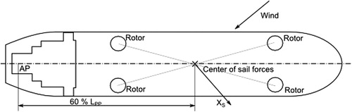
Flettner rotors with three different total sail areas were applied to the tanker. The lift and drag curves for the Flettner rotors were taken from Li et al. (2012). For each sail area, four Flettner rotors with an aspect ratio of six were included in the simulation model. Effects from shadowing and interaction between the rotors were not considered. The total force was assumed to act at one central point, 60% of Lpp from the aft perpendicular. A sketch of a possible arrangement is shown in Figure 8.

Figure 8. Sketch of a possible arrangement of the Flettner rotors on a tanker.

Optimal spin ratios were pre-computed for each apparent wind angle by maximising the power output from the sails.

A reefing function is included in the 4 DOF model which reduces the sail forces by reefing the sails. For conventional sails the sail area would then be reduced, but, for wind-assisted propulsion with Flettner rotors this would be practically accomplished by reducing (controlling) the spin ratio. A reefing factor is applied in four cases:

1. The thrust from the sails is larger than the required thrust to propel the ship at target speed.

2. The thrust from the sails is smaller than the added resistance from drift and the rudder.

3. The static heel angle exceeds 5 degrees.

4. The static rudder angle exceeds 10 degrees.

Table 2 presents results from numerical simulations with fuel savings using the 1 and 4 DOF models, with three different sail areas and 14 kn target speed. There is a difference in fuel consumption between the 1 and the 4 DOF which is around 7%. This difference is caused by the large influence of drift and rudder resistance which is not accounted for in the 1 DOF model. The results show a fuel consumption reduction of up to 20% with the largest sails. Additionally, the results show that the increase of the savings is not linear.

Table 2. Comparison of fuel consumption of the tanker with different sail configurations.

	No sail	300 m^2	600 m^2	900 m^2
1 DOF	0%	− 14%	− 23%	−27%
4 DOF	0%	− 12%	− 18%	−20%

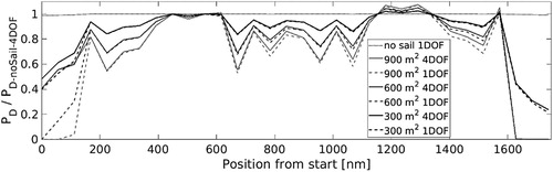
The required propulsion power with sails (1 DOF and 4 DOF), normalised with the 4 DOF power without sails, is shown in Figure 9. The huge effect of reefing, drift and rudder resistance can especially be seen in the beginning of the journey. During the first 100 nm the ship could be completely powered by the sails of 600 and 900 m², if analysed with 1 DOF. Due to large rudder angles the sail forces are reduced (i.e. the sails are reefed) causing the sails to deliver maximal 60% of the propulsion power.

Figure 9. Simulation results with different sail configurations on the tanker.

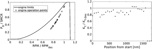
The engine and propeller working points during the journey are presented in Figure 9. During times with high sail thrust the engine can be required to be run on very low power but a still rather high rpm. This might cause problems that could be solved with a lower limit in the engine curves which is not implemented in the current version of the model. The propeller loading (KT over design KT) during times of sail assisted propulsion is typical around 80–90%, as shown in Figure 10. Considering a typical light running margin of around 5%, such a lower propeller load will cause backside cavitation. Further investigation is needed on how much backside cavitation must be avoided or until which percentage unloading the propeller could still be safely operated.

Figure 10. Engine and propeller loading with 900 m² sail area.

4. Conclusions

A new simulation model, ShipJOURNEY, developed to predict the energy consumption of ships under operational conditions, considering 4 DOF of ship motions was developed and presented. In combination with a former developed static power prediction model, ShipPOWER, the simulation model requires a minimum of information about the ship and is thus particularly applicable to studies in an early design phase, fleet optimisation studies or for ship without extensive model test results and hull/ propeller drawings available. A force and moment balance is a computed for surge, drift, yaw and heel using empirical formulas for the rudder and side forces as well as the yaw and heel moments. In the current study side forces and yaw moments from the wind on the ship and from sails were respected and compensated with the drift of the ship and a rudder angle.

Case studies with two ships, with and without auxiliary wind propulsion, showed the importance of respecting four degrees-of-freedom, especially when encountering high winds or with sails fitted to the ship. Results show differences in the fuel consumption between the 1 DOF and 4 DOF simulation of up to 2.5% for ships without sails and up to 40% with sails. It must be noted that this study focused on the differences between 1 DOF and 4 DOF simulations and not on maximising the efficiency of sails on cargo ships. To maximise the efficiency of sail assisted propulsion weather routing is compulsory. It is easily possible to couple a weather routing tool to the current model for such purpose.

It can be concluded that side forces and yaw moments must be respected when analysing or predicting the fuel consumption of ships at sea. Further on it can be concluded that sails can give high fuel saving but that large sail forces lead to high rudder forces, requiring to reef the sails or reduce the spin ratio of Flettner rotors to be able to maintain the course.

The studies have also shown that it is crucial to couple the power prediction to engine models to capture involuntary speed losses. On the example route, speed losses of up to 0.45 kn were observed for the tanker without sails. In future versions limits for, e.g. bow slamming could be implemented to capture voluntary speed loss.

At certain wind angles, Flettner rotors can provide large percentages of the propulsive power, thus leading to very low engine and propeller loads. It must be further investigated how suitable lower engine power limits can be set to avoid stalling of the engine. With respect to the propeller loading it must be investigated if pressure side cavitation, which will be unavoidable with propeller loads 5%–30% below design load, as shown in Figure 9, can be accepted or if limits for the propeller unloading must be specified. Further research must be undertaken to be able to estimate side forces and yaw moments from waves.

Disclosure statement

No potential conflict of interest was reported by the authors.

ORCID

Fabian Tillig http://orcid.org/0000-0002-9886-9147

Additional information

Funding

This work was supported by Energimyndigheten [grant number P44454-1].

Appendix 1. Detailed weather data for the journey simulation

Wind angle (TWA) and wave angle defined as degrees off bow, with 0 degree equal to head wind and waves.

Table

Distance from start (nm)	TWS (kn)	TWA (deg)	Wave height (m)	Wave angle (deg)	Water depth (m)
Eastbound journey (Gothenburg to St. Petersburg)
0	32.6	72	3.2	78	73
56	31.1	61.2	2.1	66	34
112	28.3	57.5	1.2	51	29
168	21.4	168.4	1.3	112	31
224	17.1	133.2	2.3	122	69
280	12.9	125.2	2.6	151	75
336	15.0	140.7	2.5	148	70
392	15.7	161.3	1.8	151	55
448	15.2	179.8	2.9	126	160
504	16.1	170.1	2.8	142	158
560	14.2	178.0	2.9	137	71
616	16.2	15.8	1.8	131	84
672	14.4	108.6	1.2	82	46
728	7.7	82.7	1.0	70	66
784	13.7	65.9	0.8	60	31
840	12.4	44	0.3	52	30
Westbound journey (St. Petersburg to Gothenburg)
900	12.4	136	0.3	128	30
956	13.7	114.1	0.8	120	31
1012	7.7	97.3	1.0	110	66
1068	14.4	71.4	1.2	98	46
1124	16.2	164.2	1.8	49	84
1180	14.2	2	2.9	43	71
1236	16.1	9.9	2.8	38	158
1292	15.2	0.2	2.9	54	160
1348	15.7	18.7	1.8	29	55
1404	15.0	39.3	2.5	32	70
1460	12.9	54.8	2.6	29	75
1516	17.1	46.8	2.3	58	69
1572	21.4	11.6	1.3	68	31
1628	28.3	122.5	1.2	129	29
1684	31.1	118.8	2.1	114	34
1740	32.6	08	3.2	102	73

References

- Bertram V. 2000. Practical ship hydrodynamics. Oxford: Butterworth-Heinemann.
- Blendermann W. 1994. Parameter identification of wind loads on ships. J Wind Eng Ind Aerodyn. 51(1):339–351. doi: 10.1016/0167-6105(94)90067-1
- Clarke D, Gedling P, Hine G. 1983. The application of manoeuvring criteria in hull design using linear theory. Naval Architect 45–68.
- Inoue S, Hirano M. 1981. A practical calculation method of ship manoevring motion. Int Shipbuilding Progress. 28(325): 207–222. doi: 10.3233/ISP-1981-2832502
- ITTC. 2014. Speed and power trials, part 2, analysis of speed/ power trial data. ITTC- Recommended Procedures and Guidelines. 7.5-04-01-01.2 Appen D2. http://ittc.info/media/1936/75-04-01-012.pdf.
- Kramer JA, Steen S, Savio L. 2016. Drift forces – wingsails vs Flettner rotors. High performance marine vehicles; Oct. 17th–19th; Cortuna, Italy.
- Lagarias JC, Reeds JA, Wright MA, Wright PE. 1998. Convergence properties of the Nelder-Mead simplex method in low dimensions. SIAM J Optim. 9(1):112–147. doi: 10.1137/S1052623496303470
- Lewis EW. 1989. Principles of naval architecture, second revision, volume III: motions in waves and controllability. Jersey City, NJ: SNAME.
- Schneekluth H, Bertram V. 1998. Ship design for efficiency and economy. 2nd ed. Oxford: Butterworth-Heinemann.
- Li DQ, Leer-Andersen M, Allenström B. 2012. Performance and vortex formation of Flettner rotors at high Reynolds numbers. 29th Symposium on Naval Hydrodynamics; Aug. 26th–31st; Gothenburg, Sweden.
- Naaijen P, Koster V, Dallinga RP. 2006. On the power savings by auxiliary kite propulsion. Int Shipbuilding Progress. 53:255–279.
- SMHI. 2017. Sea and coast weather [accessed 2017 December 11]. www.smhi.se/en
- Tillig F, Ringsberg JW, Mao W, Ramne B. 2017. A generic energy systems model for efficient ship design and operation. IMechE, Part M, J Eng Maritime Environ. 231(2):649–666. doi:10.1177/1475090216680672.
- Tillig F, Ringsberg JW, Mao W, Ramne B. 2018. Analysis of uncertainties in the prediction of ships’ fuel consumption – from early design to operation conditions. Ships Offsh Struct. doi: 10.1080/17445302.2018.1425519