Physical, data-driven and hybrid approaches to model engine exhaust gas temperatures in operational conditions

ABSTRACT

Fast diesel engine models for real-time prediction in dynamic conditions are required to predict engine performance parameters, to identify emerging failures early on and to establish trends in performance reduction. In order to address these issues, two main alternatives exist: one is to exploit the physical knowledge of the problem, the other one is to exploit the historical data produced by the modern automation system. Unfortunately, the first approach often results in hard-to-tune and very computationally demanding models that are not suited for real-time prediction, while the second approach is often not trusted because of its questionable physical grounds. In this paper, the authors propose a novel hybrid model, which combines physical and data-driven models, to model diesel engine exhaust gas temperatures in operational conditions. Thanks to the combination of these two techniques, the authors were able to build a fast, accurate and physically grounded model that bridges the gap between the physical and data driven approaches. In order to support the proposal, the authors will show the performance of the different methods on real-world data collected from the Holland Class Oceangoing Patrol Vessel.

KEYWORDS:

• Kernel methods
• feature mapping
• multitask learning
• condition monitoring
• hybrid models
• exhaust gas temperatures

1. Introduction

Internal combustion engines (ICEs), Diesel Engines (DEs) in particular, have been the main power provider for shipping over the past century, since their efficiency made steam engines obsolete (Curley 2012). While advanced electrical and hybrid propulsion architectures have changed propulsion systems over the past decades, the DEs maintain their primary position, either as a propulsion engine driving the shaft or as a generator providing electrical power (Geertsma, Negenborn, Visser and Hopman 2017). However, concerns over hazardous emissions from shipping on air quality (Viana et al. 2014) and on global warming (Taljegard et al. 2014) have led to more stringent regulations on emissions, such as sulfur and NO${}_x$ (IMO MARPOL 2011), and the target to reduce annual global shipping emissions with 50% by 2050 (IMO MEPC 72 2018). Economic studies suggest that internal combustion engines will maintain their leading position over the next decades (Taljegard et al. 2014), due to the long operating profiles and the high energy requirement of transport ships, although alternative fuels, such as Liquefied Natural Gas (LNG) (Anderson et al. 2015), methanol (Svanberg et al. 2018; Amma 2019) and biodiesel (Geng et al. 2017; Hoang et al. 2019) could reduce the environmental impact of engine emissions.

Hence, keeping DEs functioning and efficient is a critical issue in the marine industry for reducing the environmental impact of engine emissions and for maintaining their availability (Lloyd and Cackette 2001; Xu et al. 2002). While crews previously performed maintenance on DEs themselves, the trend to reduce crew size and the increasing complexity of ship systems have led to an increase in support contracts, through which the original equipment manufacturers perform maintenance (Ghaderi 2019). As availability requirements have also increased (Zahedi et al. 2014; Geertsma, Negenborn, Visser and Hopman 2017), maintenance needs to be accurately planned and failures before planned maintenance need to be prevented (Verbert et al. 2017). In the near future, autonomous shipping will requires even more accurate maintenance planning and increased reliability (Banda et al. 2019; Ghaderi 2019). While work on automatic path planning and collision avoidance (Liu et al. 2017, 2019) is ongoing and practical experiments have demonstrated ships sailing autonomously, the development of reliable power and propulsion systems and their operating and maintenance concepts is equally important (Schwartz 2002). Therefore, work is required to increase the reliability and the efficiency of ships power systems, in particular the main power providers such as the ICE, and to develop methods to accurately predict when maintenance is required and identify developing failures before they obstruct reliable operation (Wu et al. 2013; Cipollini et al. 2018b). In this respect, the development of a real-time virtual model of an ICE, i.e. a digital twin, that can provide accurate predictions and offer insights regarding operational performance and health status can be of great importance. This has been identified both by academia and the industry, with researchers demonstrating the benefits of this technology in a wide variety of industrial applications (Bondarenko and Fukuda 2020; Liu et al. 2020; Bhatti et al. 2021; Teng et al. 2021; Xu et al. 2021).

A critical requirement of such a virtual model for an ICE is the precise reflection of its key characteristics, under all operating conditions and in real time (Bondarenko and Fukuda 2020). Focusing on the health status of a DE, key diagnostic parameters are exhaust gas temperatures, as they can provide valuable insights, with respect to the turbocharging system, the fuel supply system, and the working medium exchange system (Korczewski 2015, 2016). More specifically, exceedingly high exhaust gas temperatures can lead to severe damage on the cylinder valves, while exceeding the permissible values in the turbine inlet cross section can cause severe and irreversible damage in the turbine blades. Considering marine engines, a number of operating conditions can potentially lead to increased exhaust gas temperatures, these include: excessive load resulting from hull fouling or damaged propeller blades, malfunction of the water cooling system that cools cylinder liners, and pollution of the exhaust manifold that is usually caused by deposits of the products of incomplete combustion.

Unfortunately, taking into account the dimensions and cost of marine DEs, the process of carrying out experimental campaigns to test the efficiency and to diagnose possible decays requires significant resources. For this reason, modelling and simulation techniques are recognised as the most effective approaches to obtain a cost-efficient and reliable understanding of the engine performance and components' interactions (Theotokatos 2010). Numerical models play a pivotal role in predicting key engine performance parameters, such as the exhaust gas temperature, to identify emerging failures early on, and to establish trends in performance degradation (Grimmelius et al. 2007). The most advanced engine models that are available in the literature (Reitz and Rutland 1995; Baldi et al. 2015; Xiang et al. 2019) show that the complexity of diesel combustion requires simulations with many complex, interacting submodels to guarantee high accuracy. However, such modelling approaches are computationally demanding, and are unsuitable for accurate and real-time dynamic predictions. As such, their use is prohibitive in applications which require real-time simulations to be performed (Khaled et al. 2014) with strict accuracy requirements under both steady-state and dynamic conditions. In order to develop accurate models that can predict engine behaviour real-time, the authors propose a Hybrid Model (HM) approach, combining both Physical Models (PMs) and Data-Driven Models (DDMs) to the problem of modelling DEs exhaust gas temperatures in operational conditions.

PMs are models in which first principle equations represent the physical phenomena of the system. The majority of studies involving PMs (see Section 2.1) report results that are in very good agreement with measurements taken from shop trial data, or under static operating conditions with a limited number of operating points. Such validation approaches might be sufficient for the purpose of the respective studies, bearing in mind possible constraints posed by the lack of available data. Nevertheless, the suitability of each model to predict key performance indicators, and in particular exhaust gas temperatures under transient operating conditions, and in true operational conditions is not sufficiently demonstrated. Moreover, the literature does not report the statistic accuracy under dynamic conditions. Finally, the most effective physical models require extensive computational time for high accuracy results.

DDMs, also called black-box models, contrarily to PMs do not exploit any first principle equations but they are able to exploit robust statistical inference procedures and historical data collected through a logging system, in order to make predictions about the future behaviour of the modelled system. DDMs have gained substantial interest with the rapid growth of ship monitoring systems within the shipping industry, and several interesting applications can be found in the literature (see Section 2.2). An advantage of these methods is represented by the fact that there is no need of any a-priori knowledge about the underlying physical system. Furthermore, thanks to the nature of these approaches, it is possible to exploit even data regarding particular phenomena that cannot be easily modelled with a PM. Despite the impressive accuracy that can be obtained, DDMs usually produce non-parametric models that are not supported by any physical interpretation; this, despite representing a possible advantage, as mentioned above, may limit the capability of the models themselves, without exploiting important knowledge about the phenomena of interest. Moreover, a great amount of historical data is necessary in order to build reliable models. In the authors' opinion, a modelling approach that aims to identify emerging failures on a DE at an early stage and establish trends with respect to performance degradation, must be able to fast and accurately predict the most critical process parameters equally well under static and dynamic operation, across the entire operating envelope providing also insight and knowledge about the physical processes.

Therefore, in this paper, an existing DE PM (Geertsma, Negenborn, Visser, Loonstijn, et al. 2017) is improved by combining PMs and DDMs (Leifsson et al. 2008; Coraddu et al. 2017). The result of this combination is a, recently named (Coraddu et al. 2018), HM, also referred to as gray-box model, which allows to exploit both the mechanistic knowledge of the physical principles and historical data. As reported in Coraddu et al. (2017), this approach provides more accurate outcomes when compared with the first principle PMs, requires a smaller amount of data when compared to the DDMs, and is extremely fast compared to advanced PMs of comparable performance. For this reason, this work aims to investigate how a combination of DDMs and PMs can improve prediction of the engine exhaust gas temperatures, using extensive measurement data from the Holland Class Oceangoing Patrol Vessel. In particular, in this paper:

• authors review the performance of a mean value PM in factory acceptance conditions, in static and dynamic conditions at sea, thus demonstrating that current state-of-the-art PMs are not suitable for predicting operating parameters in true operational conditions;

• authors test the DDMs to establish whether they can be used to predict the DE exhaust gas temperatures;

• authors present a novel HM to predict DE exhaust gas temperature combining the PMs and the DDMs mentioned above;

• authors exploit real-world data coming from a Holland Class Oceangoing Patrol Vessel to assess the accuracy and effectiveness of the different modelling approaches.

Results will demonstrate that the HM yields a more accurate representation of the DE, which will then be suitable for use in various aspects of off-line and real-time operational monitoring.

The rest of the paper is organised as follows. Section 2 gives an overview of related works. Section 3 gives a brief description of the system and reports the dataset used for this work. In Section 4, the different modelisation approaches are described, respectively the PM (see Section 4.2), the DDM (see Section 4.3) and the HM (see Section 4.4). Section 5 shows the results of the three modelling approaches on real data coming from an Holland Class Oceangoing Patrol Vessel. Finally, Section 6 summarises and concludes the paper with a description of the future scenarios opened by the authors' work.

2. Related works

In this section, the authors will review literature that deals with PMs, DDMs and HMs for DE modelling.

2.1. PMs

Intensive research has been conducted in PMs for DE modelling. The works of Grondin et al. (2004), Grimmelius et al. (2007), and Geertsma, Negenborn, Visser, Loonstijn, et al. (2017) provide insightful reviews on the extensive work done on this field, as well as its evolution over the last decades. The general consensus is that the choice of a suitable model depends primarily on the requirements of each application and, of course, the available computational tools (Johnson et al. 2010). The same is also claimed in Hountalas (2000), in which the author argues that, due to the uniqueness of marine DEs and their operation, computer programs for marine applications must be specifically designed, implying that each application needs a different model.

In Grimmelius (2003), modelling approaches for any physical system are categorised according to different dimensions; in this work, the authors will address the dimension referred to as the model level. The model level divides approaches into three groups, according to the level of detail at which the physical processes are described: PMs, DDMs and HMs. PMs, or white-box models, are the most common type adopted to deal with performance prediction, they are built considering a set of a-priori equations, defined through the knowledge of the physical phenomenon governing the DE and its performance. State-of-the-art approaches in PMs report errors well within the tolerance margins given by engine manufacturers in static conditions, however, in dynamic predictions the reported errors are much larger. Moreover, most predictions are validated in a limited operating region, mostly the operating region used for model tuning.

In Baldi et al. (2015), a combined mean value-zero dimensional model was developed and used to investigate the propulsion behaviour of a handymax-size product carrier under constant and variable engine speed operations. The modelling approach was validated against shop trials data, considering steady-state conditions with a load variation between 50% and 110%. The reported error was lower than the standard tolerance employed by the marine engine manufacturers, with a simulation time only slightly exceeding the one of the mean value model. Temperature estimation errors at compressor outlet, and turbine inlet and outlet averaged 2.7%, 1.9% and 1.5% respectively, with the lowest error margins occurring around the nominal point. They concluded that their proposed model provides a favourable time-accuracy trade-off and it can be used in cases where information, not provided by a mean-value approach, is needed. Llamas and Eriksson (2018) developed a control-oriented mean value engine model of a large two-stroke engine with Exhaust Gas Re-circulation (EGR), to assess engine performance under transient operation. The model was validated against operational data from a container-ship engine under steady-state and transient operations. For steady-state conditions 52 operating points were used, spanning a load between 10% and 90% of the nominal, with and without EGR. The stationary relative errors were reported to be in general under 3.35%, for both estimation and validation data, while the error of the temperature estimation on the exhaust manifold was recorded at a root mean square value of 12 K. Dynamic validation was performed for four different scenarios including load increase and decrease, and EGR start and stop operations. All of them were focused on low load operation, as it was the most uncertain operating area for the model. Results showed that the model was capable of following the measured engine signals during transients with low computational times, and the estimation for the exhaust manifold temperature agreed quite well with the measurements and could thus be used for control purposes. Guan et al. (2015) investigated a two-stroke marine DE with emphasis at part load operating conditions using a zero-dimensional model. The proposed model was validated against experimental data obtained from engine shop tests, which correspond to steady-state operating conditions at four different loads: 25%, 50%, 75% and 100% of the nominal. Very good accuracy was obtained for the entire operating region, and for all performance parameters. Relative percentage errors on the exhaust gas receiver temperature and the exhaust gas temperature after the turbocharger (TC) were reported to be 0.6% and 2% respectively, and errors of equal order of magnitude were observed for all process parameters.

In the work of Sui et al. (2017), a Mean Value First Principle (MVFP) model was presented with the aim of investigating performance at preliminary stage design, based on both the basic and advanced six-point Seiliger process and applicable to both steady-state and transient-state conditions. The model was validated using experimental data in three operating conditions: operation at the nominal point, 50% of nominal speed at 30% of nominal load, and 80% of nominal speed at 50% of nominal load. Although actual error values were not reported, graphical illustration of the results of the in-cylinder process showed good correspondence with the test data across all process parameters, including in-cylinder temperatures, with satisfactory accuracy and adaptability to variable operating conditions. Sapra et al. (2017) studied back pressure effects on the performance of a marine DE, by means of an MVFP model. The model was calibrated under steady-state conditions, using 9 points along a propeller curve. It was further validated at the same conditions for different back pressures. Although quantitative performance metrics for the model are not given, the graphical representation of the results indicates average relative percentage errors of around 4% for the turbine inlet temperature across all operating conditions.

In Larsen et al. (2015), the zero-dimensional model of Scappin et al. (2012) was further extended and validated for steady-state conditions within a load range of 25–100% of the nominal. The model showed good agreement with the measurements of the manufacturer across all performance parameters, with a root mean square deviation of around 1% for the exhaust gas temperature.

More recently, in Wang et al. (2020) the authors performed a parametric investigation of a large four-stoke dual-fuel marine engine in order to identify the pre-injection effects on the engine combustion, knocking and emissions parameters. Their modelling approach consisted of the integration of a 1-D model and a 3-D computational fluid dynamics (CFD) model utilising the MAN 51/60DF marine engine as a case study. The authors validated their model under steady-state conditions in 4 points, within a range of 25–100% of the nominal load. Near-zero deviation was reported for most parameters, whereas the maximum deviation for NO${}_x$ emissions was only 2.4%.

Finally, Hao et al. (2021) studies and improves the in-cylinder fuel/air mixing process of heavy-duty DEs, utilising a new device named the ‘fuel split device’. Due to the nature of their research, detailed modelling of the in-cylinder process was required, which the authors performed utilising CFD methods. To this end, they developed and verified their simulations in terms of the spray liquid/vapour penetration, heat release rate and in-cylinder pressures, at a variety of operational and environmental conditions. Although quantitative performance metrics are not explicitly given, graphical representations per crank-angle degree, show very low discrepancy between experimental and simulated results.

In summary, models are available that can accurately predict process parameters and engine temperatures. However, the most accurate models in dynamic conditions, zero dimensional models, cannot run real time, which is required to perform online condition monitoring, and this is certainly the case for more detailed CFD simulations. Alternatively, mean value models can run real time and can be used for control system design and evaluation, but lack accuracy over the complete operating envelope under dynamic conditions, as will be demonstrated in Section 5.1.

2.2. DDMs

DDMs have proved to be valuable instruments in many marine applications (Coraddu et al. 2017; Zhang et al. 2017; Cipollini et al. 2018a, 2018b; Baldini et al. 2018; Gao et al. 2018; Karimi et al. 2018; Silva et al. 2018; Yang et al. 2018), and in industry Qi et al. (2018). In particular, an older study of Antonić et al. (2004) utilised an Adaptive Neuro Fuzzy Inference System (ANFIS) to model marine DE cylinder dynamics. Experimental data from a test-bed were used, and the resulting models presented very low errors, for medium to high loads (50–100%). Porteiro et al. (2011) developed a multilayer neural network to provide load estimation and fault identification on a DE, for different faulty conditions: misfiring, shaft imbalance, clogged intake and leaking start plug, using vibration signals and exhaust temperature as inputs. The reported performance of the model, in terms of correctly classified cases, was roughly 90% using only two vibration signals for load estimation, and 89.6% for the failure type identifier. However, the work focused on mechanical failures as opposed to thermal failures that are the scope for this work. Basurko and Uriondo (2015) developed a three-layer feed-forward Artificial Neural Network (ANN) to represent the behaviour of medium speed DE with the aim of enabling a condition based maintenance framework for a fishery vessel. More than 10,000 h of operational data was utilised, with the ANN to give predictions with the mean squared error spread between 0.3 and 2.1 depending on the operational parameter. In the work of Bukovac et al. (2015), an ANN was used to replace a computationally demanding physical simulation model, and predict the steady-state performance of a two-strokes marine DE. They report that the ANN architecture did provide predictions of the same accuracy as the physical model (errors of the order of 3% compared to experimental data), while being 3000 times faster.

Furthermore, in Yu et al. (2018) a recurrent neural network for a diesel-generator set was presented, aiming at reproducing the engine output characteristics (namely rotational speed), under changes of electrical load. The model was trained using data from steady-state operations, at 25%, 50%, 75% and 100% of the nominal load. Although quantitative results were not presented, very low errors were reported across the entire operating region in steady state operations by means of graphical representations. Nikzadfar and Shamekhi (2014) utilised an ANN to study the relative contribution of several operational parameters to the performance of a DE. More specifically, the operational parameters included: injected fuel mass, pilot and main injection mass, main and pilot injection timing, inlet air pressure and temperature, exhaust pressure, fuel rail pressure and EGR, and their effects on brake torque, Soot, SO${}_x$, NO${}_x$ and specific fuel consumption were investigated. The ANN was built utilising 4000 steady-state operating points covering the entire envelope of the DE, generated by means of a simulation model. In this case too, quantitative results on the performance of the ANN are not described, however, graphical representations show a relative difference of around 5% with respect to exhaust gas temperatures. Al-Hinti et al. (2009) studied the effects of inlet air pressure on DE indicated mean effective pressure and specific fuel consumption. They introduced ANFIS as an efficient method for modelling and sensitivity analysis of a DE. Steady-state experimental data was used to develop the model, at four different air intake conditions with varying speed between 50% and 100% of the nominal. Validation results report average percentage errors of 4%, 0.15%, and 2.43% for efficiency, mean effective pressure and specific fuel consumption, respectively. Galindo et al. (2005) developed an ANN to model the combustion of high speed direct injection DEs in a transient regime. More specifically, their aim was to develop a simulation model for the rate of combustion in DEs during transient operating conditions, accurate and fast enough to be incorporated in a one-dimensional gas dynamic model for global transient behaviour prediction. Detailed analysis on the selection of the optimal architecture of the ANN was presented, with the optimal model resulting in an $R^2$ value of 0.985.

In the work of Parlak et al. (2006), an ANN was employed to model exhaust temperatures and specific fuel consumption as a function of mean effective pressure, engine speed and injection timing. The ANN was trained using experimental data at four constant engine speeds within 50–100% of the nominal speed, while varying load. The results report mean relative errors of 1.93% and 2.36%, respectively.

Another interesting application was reported in Yuanwang et al. (2002). The authors developed an ANN to analyse the effect of cetane number on exhaust emissions from a DE. The total cetane number, base cetane number and cetane improver, total cetane number and nitrogen content in the diesel fuel were used as inputs, and the emissions studied included hydrocarbon, carbon monoxide, particulate matter and NO${}_x$. The ANN was trained using 20,000 measurements, and the relative percentage errors reported ranged between 0.14% and 2.52% depending on the combination of inputs employed. Namigtle-Jiménez et al. (2019) developed an arrangement of 3 ANNs for a Fault Detection and Diagnosis scheme (FDD), based on the extraction of features from the pressure signal of the injection rail of an ICE. They showed that the proposed FDD was capable of detecting and isolating accurately the faulty injector of the electronic fuel injection system, with offline training results reporting a 100% classification accuracy in any possible fault scenario, and near 100% accurate classification in online scenarios.

A similar study was performed in Wang et al. (2019), in which the authors presented a Bayesian network-based approach for fault isolation in a DE fuel injection system, under the presence of uncertainties. Special consideration was given in the simplification of the Bayesian network structures, due to which symptoms under multiple faults could be decoupled into symptoms corresponding to each individual fault. This greatly reduced the prior knowledge needed for the diagnosis, decreased the complexity of the application, and improved the computational efficiency. Palmer and Bollas (2019) showed that model-based active Fault Detection and Isolation (FDI) tests can improve the capability of DDMs to predict and isolate faults. One of the case studies presented was the detection of actuator faults and manifold leakage on a DE. The authors showed that when proper FDI test designs are selected, even the relatively simple combination of principal component analysis and k-nearest neighbours classifier could provide satisfactory results in fault detection. Faults considered in that study included inlet and exhaust manifold leaks, variable-geometry turbine, and exhaust gas receiver actuator valve drifts.

More recently, in Wang, Chen, et al. (2021) the authors proposed a random convolutional neural network structure for health monitoring of DEs, relying on vibration measurements. More specifically, the authors constructed several individual convolutional neural networks, and the diagnostic results from each individual model were fused by a combinatorial strategy using the Dempster–Shafer evidence theory. They evaluated their approach by utilising two vibration signal datasets from a DE, and they concluded that, compared to traditional methods based on signal analysis techniques and shallow classifiers, their approach can automatically learn high-level representative features from the raw vibration signals and eliminate the necessity of manual feature extraction.

A similar approach that combines several DDMs for fault detection of DEs was proposed in Cai et al. (2020). The authors combined a rule-based algorithm with Bayesian networks, and utilising experimental data collected from an EV80 DE, they showed that their approach is able to identify seven different faults on a DE at a wide variety of rotational speeds, requiring only with few training samples at a fixed speed.

In Wang, Cai, et al. (2021), the authors proposed a diagnostic framework that integrates variational mode decomposition and the Rihaczek distribution to acquire time-frequency representations of vibration measurements of diesel engines. Utilising these features, a graph regularised bi-directional non-negative matrix factorisation algorithm was proposed to find a parts-based representation corresponding to different fault models. Their approach was compared with several other methods on an experimental dataset of the 6135G diesel engine, with a 100% fault identification accuracy, requiring few training data and high computational efficiency.

A further example is reported in Coraddu et al. (2021), in which the authors designed and proposed multiple DDMs for weakly supervised marine duel fuel engines health monitoring. The proposed framework relied on a digital twin of the engine or on novelty detection algorithms, which were compared against state-of-the-art fully supervised approaches. Utilising data from the validated simulation model of Stoumpos et al. (2020), the authors demonstrated that their approach can overcome the problematic requirement for a large amount of labelled samples, that are rarely available, with a decrease in performance of less than 1% compared to state-of-the-art fully-supervised approaches.

2.3. HMs

HMs are a quite recent modelling approach in the maritime field and just very few works showed the advantage of a hybrid approach with respect to pure PMs and DDMs. For example, in Coraddu et al. (2017) authors show that it is possible to effectively predict fuel consumption with HMs. Another example is the one reported in Miglianti et al. (2019); authors showed that it is possible to predict the propeller cavitation noise characteristics via HMs. Finally, in our preliminary work Coraddu et al. (2018), we attempt to model the engine exhaust gas temperature with a naive HM.

3. Vessel description and available data

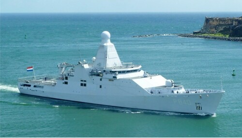
The case study Holland Class Oceangoing Patrol Vessels, shown in Figure 1, are naval vessels that can perform various security operations, such as counter terrorism, counter piracy, counter drug transport, disaster relief and coastguard operations. The small crew of 50 people requires a high degree of automation (Geertsma et al. 2013), but nevertheless maintenance load is high for the crew and needs to be reduced Horenberg and Melaet (2013). Reducing the maintenance burden on DEs using predictive maintenance based on its current sensor fit can contribute to this. The propulsion system of the vessel consists of two shafts with Controllable Pitch Propellers (CPP), a gearbox, and one DE per shaft, as shown in Figure 2. This configuration is typical for multi-function ships that require silent, maneuverable, highly reliable and low emission propulsion.

Figure 1. Holland class oceangoing patrol vessels.

The Patrol vessel is equipped with a data logging system which is used by the Royal Netherlands Navy both for on-board monitoring and control and for land-based performance analysis. For testing the developed PMs, DDMs, and HMs, the authors use the dataset of one of the two four-stroke, medium speed DEs on board. The dataset consists of 114 signals, from the on-board Integrated Platform Management System (IPMS), with a sample rate of 1/3 Hz that cover a time of 3347 h, totalling 3,988,939 data points. The dataset consists of several control and monitoring parameters of the engine, from engine speed and torque, to various operational pressures and temperatures of engine components such as the crankshaft, cylinder and turbo-charger and systems, such as water cooling, lubricating oil, exhaust-gas, and fuel systems. It should be noted that the authors consider engine performance by taking into account the interaction with gearbox, propeller and ship through the load, which is represented by measured outputs for shaft torque ($M_p$) and fuel rack position ($X_{\mathrm{g}\mathrm{o}\mathrm{v}}$). Table 1 summarises the subset of the available measurements, from the IPMS, that have been used in the modelling phase, while in Figure 3(a) schematic layout of the measured outputs is reported.

Figure 2. Propulsion system layout for the Holland class oceangoing patrol vessels.

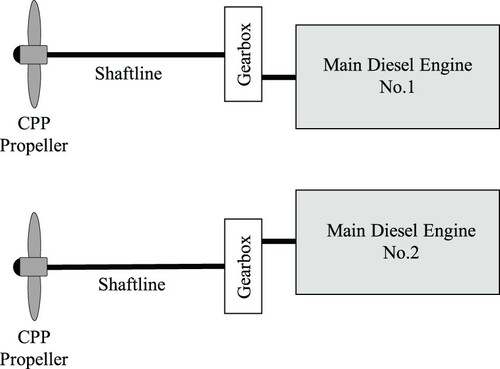
Figure 3. Schematic layout of the available data.

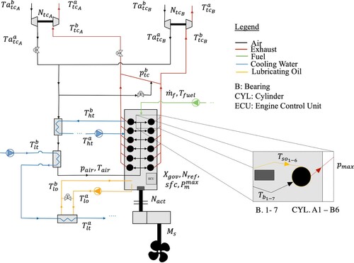
Table 1. Subset of the available measurements, from the continuous monitoring system, that have been used in the modelling phase.

Variable name	ID	Unit
Drive shaft torque	$M_s$	(Nm)
Fuel flow	${\dot{m}}_f$	(kg/s)
Turbocharger speed – Bank A	$N_{{\mathrm{t}\mathrm{c}}_A}$	(rpm)
Turbocharger speed – Bank B	$N_{{\mathrm{t}\mathrm{c}}_B}$	(rpm)
Engine speed – actuated	$N_{\mathrm{a}\mathrm{c}\mathrm{t}}$	(rpm)
Engine speed – reference	$N_{\mathrm{r}\mathrm{e}\mathrm{f}}$	(rpm)
Power margin relative to maximum	$P_m^{\mathrm{m}\mathrm{a}\mathrm{x}}$	(%)
Relative charge air pressure	$p_{\mathrm{a}\mathrm{i}\mathrm{r}}$	(bar)
Relative maximum combustion pressure	$p_{\mathrm{m}\mathrm{a}\mathrm{x}}$	(bar)
Relative pressure before turbine	$p_{\mathrm{t}\mathrm{c}}^b$	(bar)
Specific fuel oil consumption	$\mathrm{s}\mathrm{f}\mathrm{c}$	(g/kWh)
Temperature charge air	$T_{\mathrm{a}\mathrm{i}\mathrm{r}}$	(${}^{\circ }$C)
Temperature main bearing No. 1	$T_{b_1}$	(${}^{\circ }$C)
Temperature main bearing No. 2	$T_{b_2}$	(${}^{\circ }$C)
Temperature main bearing No. 3	$T_{b_3}$	(${}^{\circ }$C)
Temperature main bearing No. 4	$T_{b_4}$	(${}^{\circ }$C)
Temperature main bearing No. 5	$T_{b_5}$	(${}^{\circ }$C)
Temperature main bearing No. 6	$T_{b_6}$	(${}^{\circ }$C)
Temperature main bearing No. 7	$T_{b_7}$	(${}^{\circ }$C)
Average exhaust gas temperature – Bank A	${\overline{T}}_{{\mathrm{t}\mathrm{c}}_A}^b$	(${}^{\circ }$C]
Average exhaust gas temperature – Bank B	${\overline{T}}_{{\mathrm{t}\mathrm{c}}_B}^b$	(${}^{\circ }$C]
Fuel temperature	$T_{\mathrm{f}\mathrm{u}\mathrm{e}\mathrm{l}}$	(${}^{\circ }$C)
High-temperature cooling water temperature after cooler	$T_{\mathrm{h}\mathrm{t}}^a$	(${}^{\circ }$C)
High-temperature cooling water temperature before cooler	$T_{\mathrm{h}\mathrm{t}}^b$	(${}^{\circ }$C)
Lube oil temperature before engine	$T_{\mathrm{l}\mathrm{o}}^b$	(${}^{\circ }$C)
Lube oil temperature after engine	$T_{\mathrm{l}\mathrm{o}}^a$	(${}^{\circ }$C)
Low-temperature cooling water temperature after cooler	$T_{\mathrm{l}\mathrm{t}}^a$	(${}^{\circ }$C)
Low-temperature cooling water temperature before cooler	$T_{\mathrm{l}\mathrm{t}}^b$	(${}^{\circ }$C)
Temperature splash oil compartment 1	$T_{{\mathrm{s}\mathrm{o}}_1}$	(${}^{\circ }$C)
Temperature splash oil compartment 2	$T_{{\mathrm{s}\mathrm{o}}_2}$	(${}^{\circ }$C)
Temperature splash oil compartment 3	$T_{{\mathrm{s}\mathrm{o}}_3}$	(${}^{\circ }$C)
Temperature splash oil compartment 4	$T_{{\mathrm{s}\mathrm{o}}_4}$	(${}^{\circ }$C)
Temperature splash oil compartment 5	$T_{{\mathrm{s}\mathrm{o}}_5}$	(${}^{\circ }$C)
Temperature splash oil compartment 6	$T_{{\mathrm{s}\mathrm{o}}_6}$	(${}^{\circ }$C)
Charge air temperature after compressor – Bank A	$T{a}_{{\mathrm{t}\mathrm{c}}_A}^a$	(${}^{\circ }$C)
Charge air temperature after compressor – Bank B	$T{a}_{{\mathrm{t}\mathrm{c}}_B}^a$	(${}^{\circ }$C)
Charge air temperature before compressor – Bank A	$T{a}_{{\mathrm{t}\mathrm{c}}_A}^b$	(${}^{\circ }$C)
Charge air temperature before compressor – Bank B	$T{a}_{{\mathrm{t}\mathrm{c}}_B}^b$	(${}^{\circ }$C)
Exhaust gas temperature after turbine – Bank A	$T_{{\mathrm{t}\mathrm{c}}_A}^a$	(${}^{\circ }$C)
Exhaust gas temperature after turbine – Bank B	$T_{{\mathrm{t}\mathrm{c}}_B}^a$	(${}^{\circ }$C)
Exhaust gas temperature before turbine – Bank A	$T_{{\mathrm{t}\mathrm{c}}_A}^b$	(${}^{\circ }$C)
Exhaust gas temperature before turbine – Bank B	$T_{{\mathrm{t}\mathrm{c}}_B}^b$	(${}^{\circ }$C)
Fuel rack position	$X_{\mathrm{g}\mathrm{o}\mathrm{v}}$	(%)

4. Modelisation

In the proposed context, namely modelling DE exhaust gas temperatures in operational conditions, a general modelisation framework can be defined, characterised by an input space $\mathcal{X}\subseteq {\mathbb{R}}^d$, an output space $\mathcal{Y}\subseteq \mathbb{R}$, and an unknown relation $\mu :\mathcal{X}\to \mathcal{Y}$ to be learned. For what concerns this work, $\mathcal{X}$ is composed by the features reported in Table 2, while the output space $\mathcal{Y}$ refers to the exhaust gas temperatures reported in Table 3.

Table 2. Input space $\mathcal{X}$ for the modelisation phase.

$M_s$	${\dot{m}}_f$	$N_{{\mathrm{t}\mathrm{c}}_A}$	$N_{{\mathrm{t}\mathrm{c}}_B}$	$N_{\mathrm{a}\mathrm{c}\mathrm{t}}$	$N_{\mathrm{r}\mathrm{e}\mathrm{f}}$
$P_m^{\mathrm{m}\mathrm{a}\mathrm{x}}$	$p_{\mathrm{a}\mathrm{i}\mathrm{r}}$	$p_{\mathrm{m}\mathrm{a}\mathrm{x}}$	$p_{\mathrm{t}\mathrm{c}}^b$	$\mathrm{s}\mathrm{f}\mathrm{c}$	$T_{\mathrm{a}\mathrm{i}\mathrm{r}}$
$T_{b_1}$	$T_{b_2}$	$T_{b_3}$	$T_{b_4}$	$T_{b_5}$	$T_{b_6}$
$T_{b_7}$	$T_{\mathrm{f}\mathrm{u}\mathrm{e}\mathrm{l}}$	$T_{\mathrm{h}\mathrm{t}}^a$	$T_{\mathrm{h}\mathrm{t}}^b$	$T_{\mathrm{l}\mathrm{o}}^b$	$T_{\mathrm{l}\mathrm{o}}^a$
$T_{\mathrm{l}\mathrm{t}}^a$	$T_{\mathrm{l}\mathrm{t}}^b$	$T_{{\mathrm{s}\mathrm{o}}_1}$	$T_{{\mathrm{s}\mathrm{o}}_2}$	$T_{{\mathrm{s}\mathrm{o}}_3}$	$T_{{\mathrm{s}\mathrm{o}}_4}$
$T_{{\mathrm{s}\mathrm{o}}_5}$	$T_{{\mathrm{s}\mathrm{o}}_6}$	$T_{{\mathrm{t}\mathrm{c}}_A}^a$	$T_{{\mathrm{t}\mathrm{c}}_B}^a$	$T_{{\mathrm{t}\mathrm{c}}_A}^b$	$T_{{\mathrm{t}\mathrm{c}}_B}^b$
$T_{c_A}^a$	$T_{c_B}^a$	$T_{c_A}^b$	$T_{c_B}^b$	$X_{\mathrm{g}\mathrm{o}\mathrm{v}}$

Table 3. Output space $\mathcal{Y}$ for the modelisation phase.

${\overline{T}}_{\mathrm{t}\mathrm{c}}^a=\frac{1}{2}(T_{{\mathrm{t}\mathrm{c}}_A}^a+T_{{\mathrm{t}\mathrm{c}}_B}^a)$

${\overline{T}}_{\mathrm{t}\mathrm{c}}^b=\frac{1}{2}(T_{{\mathrm{t}\mathrm{c}}_A}^b+T_{{\mathrm{t}\mathrm{c}}_B}^b)$

In this context, the authors define as model $h:\mathcal{X}\to \mathcal{Y}$ an artificial simplification of μ. The model h can be obtained with different kinds of techniques, for example requiring some physical knowledge of the problem, as in PMs, or the acquisition of large amount of data, as in DDMs, or both of them, as in HMs.

4.1. Performance measures

Independently of the adopted technique, any model h requires some data in order to be tuned (or learned) on the problem specificity and to be validated (or tested) on a real-world scenario. For these purposes, two separate sets of data ${\mathcal{D}}_n=\left\{\right({\mathit{x}}_1,y_1),\dots ,({\mathit{x}}_n,y_n\left)\right\}$ and ${\mathcal{T}}_m=\left\{\right({\mathit{x}}_1^t,y_1^t),\dots ,({\mathit{x}}_m^t,y_m^t\left)\right\}$, where $X\in \mathcal{X}$ and $Y\in \mathcal{Y}$, need to be exploited, to respectively tune h and evaluate its performances. It is important to note that ${\mathcal{T}}_m$ is needed since the error that h would commit over ${\mathcal{D}}_n$ would be too optimistically biased since ${\mathcal{D}}_n$ has been used to tune h.

Hence, the error that h commits on ${\mathcal{T}}_m$ in approximating the real process is usually measured with reference to different indexes of performance (Ghelardoni et al. 2013):

• the Mean Absolute Error (MAE) is computed by taking the absolute loss value of h over ${\mathcal{T}}_m$ (1) $\mathrm{M}\mathrm{A}\mathrm{E}\left(h\right)=\frac{1}{m}\sum _{i=1}^m\left|h\right({\mathit{x}}_i^t)-y_i^t|;$(1)

• the Mean Absolute Percentage Error (MAPE) is computed by taking the absolute loss value of h over ${\mathcal{T}}_m$ in percentage (2) $\mathrm{M}\mathrm{A}\mathrm{P}\mathrm{E}\left(h\right)=\frac{100}{m}\sum _{i=1}^m\left|\frac{h\left({\mathit{x}}_i^t\right)-y_i^t}{y_i^t}\right|;$(2)

• the Pearson Product-Moment Correlation Coefficient (PPMCC) measures the linear dependency between $h\left({\mathit{x}}_i^t\right)$ and $y_i^t$ with $i\in \{1,\dots ,m\}$ (3) $\mathrm{P}\mathrm{P}\mathrm{M}\mathrm{C}\mathrm{C}\left(h\right)=\frac{\sum _{i=1}^m(y_i^t-\overline{y})\left(h\right({\mathit{x}}_i^t)-\hat{\overline{y}})}{\sqrt{\sum _{i=1}^m(y_i^t-\overline{y}{)}^2}\sqrt{\sum _{i=1}^m\left(h\right({\mathit{x}}_i^t)-\hat{\overline{y}}{)}^2}},$(3) where $\overline{y}=\frac{1}{m}\sum _{i=1}^m{y}_i^t$ and $\hat{\overline{y}}=\frac{1}{m}\sum _{i=1}^{m}h\left({\mathit{x}}_i^t\right)$.

Other measures of error exist, such as R-squared and the Mean Square Error. However, in this work the authors consider these three measures because, from a physical point of view, they give a complete description of the quality of the model, and adding more measures would make the results more difficult to interpret while not adding any new insights.

4.2. Physical models (PMs)

The PM used in this work is illustrated in Figure 4. It is a Mean Value Engine Model (MVEM), and a slightly improved version of the one described in Geertsma, Negenborn, Visser, Loonstijn, et al. (2017). The MVEM was developed to investigate the performance of the ship propulsion system and its control strategy, with respect to fuel consumption; acceleration time and minimum air excess ratio, during predefined acceleration manoeuvres at varying operating conditions (Geertsma, Negenborn, Visser and Hopman 2017). As many other engine models, the MVEM was calibrated against the Factory Acceptance Test (FAT) protocol and showed a mean absolute percentage error within 10%, as reported in Figure 6. For the purpose of control strategy evaluation, the MVEM provided good resemblance with the measured system behaviour, but its accuracy was never reported with any statistically robust measures. For this reason, in Section 5.1, the authors will re-evaluate the model performance on the large dataset presented in Section 3, considering the following scenarios:

• Steady state: The data described in Section 3 will be used to prove the MVEM limitations in predicting exhaust gas temperature in real world application characterised by steady-state conditions.

• Transient: the remaining part of the data, described in Section 3, will be used to further assess the MVEM limitations in transient conditions.

In subsequent works, the MVEM was used to evaluate advanced control strategies for mechanical (Geertsma et al. 2018) and hybrid propulsion architectures (Geertsma, Negenborn, Visser and Hopman 2017), hybrid propulsion systems, and hybrid power supply architectures (Kalikatzarakis et al. 2018). As these studies considered benchmark ship manoeuvres (Geertsma, Negenborn, Visser and Hopman 2017; Geertsma et al. 2018) and fuel consumption over a typical operating profile (Kalikatzarakis et al. 2018), these studies exploited the main feature of the MVEM: runtimes between 100 and 2500 times real-time (Geertsma et al. 2018). This also enables to test the performance of this model on the dataset described in Section 3 and to develop the HMs detailed in Section 4.4.

Figure 4. Schematic representation of the DE model and the interaction of its subsystems, from Geertsma, Negenborn, Visser, Loonstijn, et al. (2017).

The MVEM consists of three state variables: fuel injection per cylinder per cycle $m_f$, charge pressure $p_{\mathrm{a}\mathrm{i}\mathrm{r}}$ and exhaust receiver pressure $p_{\mathrm{t}\mathrm{c}}^b$. The inputs of the model are engine speed $N_{\mathrm{r}\mathrm{e}\mathrm{f}}$ and fuel pump set-point $X_{\mathrm{s}\mathrm{e}\mathrm{t}}$, the latter originating from the speed governor, and the output is engine torque $M_e$.

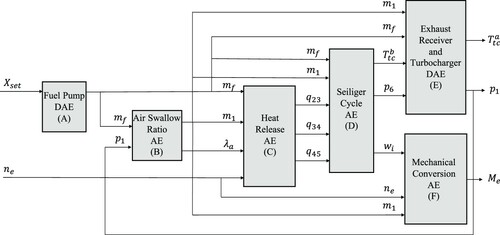
The model is characterised by six modules, as illustrated in Figure 4 and described below.

(A)	the fuel pump module represents the combined effect of the fuel pump inertia and the ignition delay;
(B)	the air swallow module represents the air swallow characteristics of the engine to establish the air excess ratio ${\lambda }_a$, the amount of air that is left after all fuel is combusted. The air excess ratio can be used as an indicator for engine thermal loading (Sapra et al. 2017) and EGR effectiveness (Asad and Zheng 2014; Nielsen et al. 2017; Llamas and Eriksson 2018);
(C)	the heat release module represents the heat release during combustion of fuel during the three combustion stages in the Seiliger cycle: isochoric, isobaric and isothermal combustion;
(D)	the Seiliger cycle module represents in-cylinder compression, combustion and expansion using the six stage Seiliger process. It establishes the work produced during the closed cylinder process $w_i$, the temperature $T_{\mathrm{t}\mathrm{c}}^b$ and pressure $p_6$ at the end of the closed cylinder process, when the exhaust valve opens;
(E)	the exhaust receiver and TC module represents Zinner blowdown (Zinner 1980) and the Büchi power and flow balance (Dixon 1998; Stapersma 2010) with variable TC efficiency, heat release efficiency and slip ratio. This module establishes the charge pressure $p_1$ and the exhaust receiver pressure $p_{\mathrm{t}\mathrm{c}}^b$. Furthermore, thermal inertias have been added to account for the effect of the location of the thermocouples, mounted on the surface of the exhaust pipes, as reported in Figure 3. The authors have included thermal inertia effects by means of a first order response with a thermocouple time constant, ${\tau }_{\mathrm{t}\mathrm{c}}$, and a constant bias, $b_{\mathrm{t}\mathrm{c}}$, to better align the physical prediction with the actual temperature measurements. The output of the module are the exhaust gas temperature at TC inlet (a), $T_{\mathrm{t}\mathrm{c}}^a$ and TC outlet (b) $T_{\mathrm{t}\mathrm{c}}^b$ (4) $\frac{T_{\mathrm{t}\mathrm{c}}^b\left(t\right)}{dt}=\frac{\left(T_{\mathrm{t}\mathrm{c}}^b\right(t-1)-b_{\mathrm{t}\mathrm{c}}^b)-T_{\mathrm{t}\mathrm{c}}^b\left(t\right)}{{\tau }_{\mathrm{t}\mathrm{c}}^b},$(4) (5) $\frac{T_{\mathrm{t}\mathrm{c}}^a\left(t\right)}{dt}=\frac{\left(T_{\mathrm{t}\mathrm{c}}^a\right(t-1)-b_{\mathrm{t}\mathrm{c}}^a)-T_{\mathrm{t}\mathrm{c}}^a\left(t\right)}{{\tau }_{\mathrm{t}\mathrm{c}}^a};$(5)
(F)	the mechanical conversion module represents the mechanical losses due to the conversion from pressure to rotation and the losses due to driving auxiliary equipment.

For a more detailed description of the modules, the reader is referred to Geertsma et al. (2018).

In summary, the temperatures of the gas flow in the exhaust receiver and at the turbine exit, main subjects of this study, are represented by a system of Algebraic Equations (AE) and Differential and Algebraic Equations (DAE) featuring the input variables, state variables and the following mathematically related parameters: trapped mass in the cylinder $m_1$, air excess ratio ${\lambda }_a$, isobaric, isochoric and isothermal heat release $q_{23}$, $q_{34}$ and $q_{45}$, temperature and pressure after expansion of the Seiliger cycle $T_{\mathrm{t}\mathrm{c}}^b$ and $p_6$ and induced work during the Seiliger cycle $w_i$. The original aspect of this model is that the TC dynamics are represented by the Büchi power and flow balance between compressor and turbine, and do not require compressor or turbine maps for calibration. By neglecting fast dynamics, the model's run-time is between 100 and 2500 times real-time, much faster than MVEMs using compressor and turbine maps, such as Nielsen et al. (2017), Theotokatos and Tzelepis (2015), Sapra et al. (2017), and Kökkülünk et al. (2016).

Lastly, in order to compare the real measurements from the IPMS with the PM outcomes, the authors considered the average value of the Bank A and B (6) ${\overline{T}}_{\mathrm{t}\mathrm{c}}^b=\frac{T_{{\mathrm{t}\mathrm{c}}_A}^b+T_{{\mathrm{t}\mathrm{c}}_B}^b}{2},{\overline{T}}_{\mathrm{t}\mathrm{c}}^a=\frac{T_{{\mathrm{t}\mathrm{c}}_A}^a+T_{{\mathrm{t}\mathrm{c}}_B}^a}{2}.$(6)

4.3. Data driven models (DDMs)

The problem considered here, from the data science point of view, can be mapped to a typical Machine Learning (ML) regression problem (Vapnik 1998; Shawe-Taylor and Cristianini 2004) in a straightforward approach. In fact, ML techniques aim at estimating the unknown relationship μ between input and output through a learning algorithm ${\mathcal{A}}_{\mathcal{H}}$ which exploits the data in ${\mathcal{D}}_n$ to learn h and where $\mathcal{H}$ is a set of hyperparameters which characterises the generalisation performance of $\mathcal{A}$ (Oneto 2020).

In this paper, a method from the ML Kernel Methods family called Kernel Regularised Least Squares (KRLS) has been adopted in order to estimate the relation between the input variables of Table 2 and the output variables of Table 3. The idea behind KRLS can be summarised as follows. During the training phase, the quality of the learned function $h\left(\mathit{x}\right)$ is measured according to a loss function $\ell \left(h\right(\mathit{x}),y)$ (Rosasco et al. 2004) with the empirical error (7) ${\hat{L}}_n\left(h\right)=\frac{1}{n}\sum _{i=1}^n\ell \left(h\right({\mathit{x}}_i),y_i).$(7) A simple criterion for selecting the final model during the training phase could then consist in simply choosing the approximating function that minimises the empirical error ${\hat{L}}_n\left(h\right)$. This approach is known as Empirical Risk Minimisation (ERM) (Vapnik 1998). However, ERM is usually avoided in ML as it leads to severe overfitting of the model on the training dataset. As a matter of fact, in this case the training process could choose a model, complicated enough to perfectly describe all the training samples (including noise, which afflicts them). In other words, ERM implies memorisation of data rather than learning from them.

A more effective approach is to minimise a cost function where the tradeoff between accuracy on the training data and a measure of the complexity of the selected model is achieved (Tikhonov and Arsenin 1979), implementing the Occam's razor principle (8) $h^{\ast }:\underset{h}{min}{\hat{L}}_n\left(h\right)+\lambda C\left(h\right).$(8) In other words, the best approximating function $h^{\ast }$ is chosen as the one that is complicated enough to learn from data without overfitting them. In particular, $C\left(\cdot \right)$ is a complexity measure: depending on the exploited ML approach, different measures are realised. Instead, $\lambda \in [0,\mathrm{\infty })$ is a hyperparameter, that must be set a-priori and is not obtained as an output of the optimisation procedure: it regulates the trade-off between the overfitting tendency, related to the minimisation of the empirical error, and the underfitting tendency, related to the minimisation of $C\left(\cdot \right)$. The optimal value for λ is problem-dependent, and tuning this hyperparameter is a non-trivial task, as will be discussed later in this section. In KRLS, models are defined as (9) $h\left(\mathit{x}\right)={\mathit{w}}^T\mathit{\phi }\left(\mathit{x}\right),$(9) where $\mathit{\phi }$ is an a-priori defined Feature Mapping (FM) (Shalev-Shwartz and Ben-David 2014), which strongly depends on the particular problem under examination and will be described later in this section, allowing to keep the structure of $h\left(\mathit{x}\right)$ linear. The complexity of the models, in KRLS, is measured as (10) $C\left(h\right)=\Vert \mathit{w}{\Vert }^2,$(10) i.e. the Euclidean norm of the set of weights describing the regressor, which is a standard complexity measure in ML (Shalev-Shwartz and Ben-David 2014). Regarding the loss function, the square loss is typically adopted because of its convexity, smoothness, and statistical properties (Rosasco et al. 2004) (11) ${\hat{L}}_n\left(h\right)=\frac{1}{n}\sum _{i=1}^n\ell \left(h\right({\mathit{x}}_i),y_i)=\frac{1}{n}\sum _{i=1}^n\left[h\right({\mathit{x}}_i)-y_i{]}^2.$(11) Consequently, Problem (8(8) $h^{\ast }:\underset{h}{min}{\hat{L}}_n\left(h\right)+\lambda C\left(h\right).$(8) ) can be reformulated as (12) ${\mathit{w}}^{\ast }:\underset{\mathit{w}}{min}\sum _{i=1}^n\left[{\mathit{w}}^T\mathit{\phi }\right(\mathit{x})-y_i{]}^2+\lambda \Vert \mathit{w}{\Vert }^2.$(12) By exploiting the Representer Theorem (Schölkopf et al. 2001), the solution $h^{\ast }$ of the RLS Problem (12(12) ${\mathit{w}}^{\ast }:\underset{\mathit{w}}{min}\sum _{i=1}^n\left[{\mathit{w}}^T\mathit{\phi }\right(\mathit{x})-y_i{]}^2+\lambda \Vert \mathit{w}{\Vert }^2.$(12) ) can be expressed as a linear combination of the samples projected in the space defined by $\mathit{\phi }$ (13) $h^{\ast }\left(\mathit{x}\right)=\sum _{i=1}^n{\alpha }_i\mathit{\phi }\left({\mathit{x}}_i{)}^T\mathit{\phi }\right(\mathit{x}).$(13) It is worth underlining that, according to the kernel trick, it is possible to reformulate $h^{\ast }\left(\mathit{x}\right)$ without an explicit knowledge of $\mathit{\phi }$, and consequently avoiding the course of dimensionality of computing $\mathit{\phi }$, by using a proper kernel function $K({\mathit{x}}_i,\mathit{x})=\mathit{\phi }\left({\mathit{x}}_i{)}^T\mathit{\phi }\right(\mathit{x})$ (14) $h^{\ast }\left(\mathit{x}\right)=\sum _{i=1}^n{\alpha }_{i}K({\mathit{x}}_i,\mathit{x}).$(14) Several kernel functions can be retrieved in literature (Cristianini and Shawe-Taylor 2000; Scholkopf 2001), each one with a particular property that can be exploited based on the problem under exam.

The KRLS problem of Equation (12(12) ${\mathit{w}}^{\ast }:\underset{\mathit{w}}{min}\sum _{i=1}^n\left[{\mathit{w}}^T\mathit{\phi }\right(\mathit{x})-y_i{]}^2+\lambda \Vert \mathit{w}{\Vert }^2.$(12) ) can be reformulated by exploiting kernels as (15) ${\mathit{\alpha }}^{\ast }:\underset{\mathit{\alpha }}{min}\Vert Q\mathit{\alpha }-\mathit{y}{\Vert }^2+\lambda {\mathit{\alpha }}^{T}Q\mathit{\alpha },$(15) where $\mathit{y}=[y_1,\dots ,y_n{]}^{\mathrm{T}}$, $\mathit{\alpha }=[{\alpha }_1,\dots ,{\alpha }_n{]}^{\mathrm{T}}$, the matrix Q such that $Q_{i,j}=K({\mathit{x}}_j,{\mathit{x}}_i)$, and the identity matrix $I\in {\mathbb{R}}^{n\times n}$. By setting the gradient equal to zero w.r.t. $\mathit{\alpha }$ it is possible to state that (16) $(Q+\lambda I){\mathit{\alpha }}^{\ast }=\mathit{y},$(16) which is a linear system for which effective solvers have been developed over the years, allowing it to cope with even very large sets of training data (Young 2003).

The problems that still have to be faced is how to choose $\mathit{\phi }$, the kernel K, and how to set up the hyperparameter λ. It is possible to start by setting $\mathit{\phi }$ and the kernel K. Usually the Gaussian kernel is exploited in real world applications because of the theoretical reasons described in Keerthi and Lin (2003) and because of its effectiveness (Fernández-Delgado et al. 2014; Wainberg et al. 2016). Basically the Gaussian kernel is able to implicitly create an infinite dimensional $\mathit{\phi }$ and thanks to this, the KRLS are able to learn any possible function (Keerthi and Lin 2003). The last problem is how to tune the hyperparameters γ, and λ of the proposed method.

Since every ML model is characterised by a set of hyperparameters $\mathcal{H}$, influencing their ability to estimate μ, a proper Model Selection (MS) procedure needs to be adopted (Oneto 2020). Several methods exist for MS purpose but resampling methods, like the well-known k-Fold Cross Validation (KCV) (Kohavi 1995) or the nonparametric Bootstrap (BTS) (Efron and Tibshirani 1994) approaches, representing the state-of-the-art MS approaches when targeting real-world applications. Resampling methods rely on the following method: the original dataset ${\mathcal{D}}_n$ is resampled once or many ($n_r$) times, with or without replacement, to build two independent datasets called the training, and the validation sets, respectively ${\mathcal{L}}_l^r$ and ${\mathcal{V}}_v^r$, with $r\in \{1,\dots ,n_r\}$. Note that ${\mathcal{L}}_l^r\cap {\mathcal{V}}_v^r=\oslash$, ${\mathcal{L}}_l^r\cup {\mathcal{V}}_v^r={\mathcal{D}}_n$. Then, in order to select the best combination the hyperparameters $\mathcal{H}$ in a set of possible ones $\mathfrak{H}=\{{\mathcal{H}}_1,{\mathcal{H}}_2,\dots \}$ for the algorithm ${\mathcal{A}}_{\mathcal{H}}$ or, in other words, to perform the MS phase, the following procedure has to be applied: (17) ${\mathcal{H}}^{\ast }:\underset{\mathcal{H}\in \mathfrak{H}}{min}{\displaystyle \frac{1}{n_r}\sum _{r=1}^{n_r}{\displaystyle \frac{1}{v}\sum _{({\mathit{x}}_i,y_i)\in {\mathcal{V}}_v^r}\ell \left({\mathcal{A}}_{\mathcal{H},{\mathcal{L}}_l^r}\right({\mathit{x}}_i),y_i),}}$(17) where ${\mathcal{A}}_{\mathcal{H},{\mathcal{L}}_l^r}$ is a model built with the algorithm $\mathcal{A}$ with its set of hyperparameters $\mathcal{H}$ and with the data ${\mathcal{L}}_l^r$. Since the data in ${\mathcal{L}}_l^r$ are independent from the ones in ${\mathcal{V}}_v^r$, the idea is that ${\mathcal{H}}^{\ast }$ should be the set of hyperparameters which allows to achieve a small error on a data set that is independent from the training set.

In this work, authors will exploit the BTS procedure and consequently r=500, if l=n and the resampling must be done with replacement (Oneto 2020).

4.4. Hybrid models (HMs)

The problem that authors face is how to construct a model able to take both, the physical knowledge about the problem encapsulated in the PMs of Section 4.2 and the information hidden in the available data as the DDMs of Section 4.3, into account. For this purpose authors will start from a simple observation: a HM, based on the previous observation, should be able to learn from the data without being too different, or too far away, from the PM.

From the Data Science point of view, this requirement can be straightforwardly mapped in a typical ML Multi Task Learning (MTL) problem (Caruana 1997; Baxter 2000; Bakker and Heskes 2003; Evgeniou and Pontil 2004; Argyriou et al. 2008). MTL aims at simultaneously learning two concepts, in this case the PM and the available data, through a learning algorithm ${\mathcal{A}}_{\mathcal{H}}$ which exploits the data in ${\mathcal{D}}_n$ to learn a function h which is both close to the observation, the data ${\mathcal{D}}_n$ and the PM, namely its forecasts.

Consequently, in this case a slightly different scenario is presented where the dataset is composed by a triple of points ${\mathcal{D}}_n=\left\{\right({\mathit{x}}_1,y_1,p_1),\dots ,({\mathit{x}}_n,y_n,p_n\left)\right\}$ where $p_i$ is the output of the PM in the point ${\mathit{x}}_n$ with $i\in \{1,\dots ,n\}$. The target is to learn a function able to approximate both μ, namely the relation between the input $\mathit{x}\in \mathcal{X}$ and the output $y\in \mathcal{Y}$, and the PM, namely the relation between the input and the output of the PM. Two tasks have to be learned. For this purpose, there are two main approaches: the first approach is called Shared Task Learning (STL) and the second Independent Task Learning (ITL). While the latter independently learns a different model for each task, the former aims to learn a model that is common between all tasks. A well-known weakness of these methods is that they tend to generalise poorly on one of the two tasks (Baxter 2000). In this paper, authors show that an appealing approach to overcome such limitations is provided by MTL (Caruana 1997; Baxter 2000; Bakker and Heskes 2003; Evgeniou and Pontil 2004; Argyriou et al. 2008). This methodology leverages on the information between the tasks to learn more accurate models.

In order to apply the MTL approach to this case, it is possible to modify the KRLS problem of Equation (12(12) ${\mathit{w}}^{\ast }:\underset{\mathit{w}}{min}\sum _{i=1}^n\left[{\mathit{w}}^T\mathit{\phi }\right(\mathit{x})-y_i{]}^2+\lambda \Vert \mathit{w}{\Vert }^2.$(12) ) in order to simultaneously learn a shared model and a task specific model which should be close to the shared model. In this way, authors obtain a model which is able to simultaneously learn the two tasks. The model that authors are interested in is the shared model, while the task specific models are just used as a tool. A shared model is defined as (18) $h\left(\mathit{x}\right)={\mathit{w}}^T\mathit{\phi }\left(\mathit{x}\right),$(18) and two task specific models as (19) $h_i\left(\mathit{x}\right)={\mathit{w}}_i^T\mathit{\phi }\left(\mathit{x}\right),i\in \{y,p\}.$(19) Then, it is possible to state the MTL version of Equation (12(12) ${\mathit{w}}^{\ast }:\underset{\mathit{w}}{min}\sum _{i=1}^n\left[{\mathit{w}}^T\mathit{\phi }\right(\mathit{x})-y_i{]}^2+\lambda \Vert \mathit{w}{\Vert }^2.$(12) ), as follows: (20) $\begin{array}{rl}{\mathit{w}}^{\ast },{\mathit{w}}_y^{\ast },{\mathit{w}}_p^{\ast }:& \underset{\mathit{w},{\mathit{w}}_y,{\mathit{w}}_p}{min}\sum _{i=1}^n\left[{\mathit{w}}^T\mathit{\phi }\right(\mathit{x})-y_i{]}^2+[{\mathit{w}}^T\mathit{\phi }\left(\mathit{x}\right)-p_i{]}^2\\ & +\sum _{i=1}^n\left[{\mathit{w}}_y^T\mathit{\phi }\right(\mathit{x})-y_i{]}^2+[{\mathit{w}}_p^T\mathit{\phi }\left(\mathit{x}\right)-p_i{]}^2\\ & +\lambda \Vert \mathit{w}{\Vert }^2+\theta (\Vert \mathit{w}-{\mathit{w}}_y{\Vert }^2+\Vert \mathit{w}-{\mathit{w}}_p{\Vert }^2),\end{array}$(20) where λ is the usual regularisation of KRLS and $\theta \in [0,\mathrm{\infty })$, instead, is another hyperparameter that forces the shared model to be close to the task specific models. Basically the MTL problem of Equation (20(20) $\begin{array}{rl}{\mathit{w}}^{\ast },{\mathit{w}}_y^{\ast },{\mathit{w}}_p^{\ast }:& \underset{\mathit{w},{\mathit{w}}_y,{\mathit{w}}_p}{min}\sum _{i=1}^n\left[{\mathit{w}}^T\mathit{\phi }\right(\mathit{x})-y_i{]}^2+[{\mathit{w}}^T\mathit{\phi }\left(\mathit{x}\right)-p_i{]}^2\\ & +\sum _{i=1}^n\left[{\mathit{w}}_y^T\mathit{\phi }\right(\mathit{x})-y_i{]}^2+[{\mathit{w}}_p^T\mathit{\phi }\left(\mathit{x}\right)-p_i{]}^2\\ & +\lambda \Vert \mathit{w}{\Vert }^2+\theta (\Vert \mathit{w}-{\mathit{w}}_y{\Vert }^2+\Vert \mathit{w}-{\mathit{w}}_p{\Vert }^2),\end{array}$(20) ) is a concatenation of three learning problems solved with KRLS plus a term which tries to keep a relation between all the three different problems.

By exploiting the kernel trick as in KRLS, it is possible to reformulate Problem (20(20) $\begin{array}{rl}{\mathit{w}}^{\ast },{\mathit{w}}_y^{\ast },{\mathit{w}}_p^{\ast }:& \underset{\mathit{w},{\mathit{w}}_y,{\mathit{w}}_p}{min}\sum _{i=1}^n\left[{\mathit{w}}^T\mathit{\phi }\right(\mathit{x})-y_i{]}^2+[{\mathit{w}}^T\mathit{\phi }\left(\mathit{x}\right)-p_i{]}^2\\ & +\sum _{i=1}^n\left[{\mathit{w}}_y^T\mathit{\phi }\right(\mathit{x})-y_i{]}^2+[{\mathit{w}}_p^T\mathit{\phi }\left(\mathit{x}\right)-p_i{]}^2\\ & +\lambda \Vert \mathit{w}{\Vert }^2+\theta (\Vert \mathit{w}-{\mathit{w}}_y{\Vert }^2+\Vert \mathit{w}-{\mathit{w}}_p{\Vert }^2),\end{array}$(20) ), as follows: (21) $\begin{array}{rl}{\mathit{\alpha }}^{\ast }:& \underset{\mathit{\alpha }}{min}{\Vert \left[\begin{array}{ccc}Q& Q0& 0\\ Q& Q0& 0\\ 0& 0Q& 0\\ 0& 00& Q\end{array}\right]\mathit{\alpha }-\left[\begin{array}{c}\mathit{y}\\ \mathit{p}\\ \mathit{y}\\ \mathit{p}\end{array}\right]\Vert }^2\\ & +{\mathit{\alpha }}^T\left[\begin{array}{cccc}(\lambda +2\theta )Q& (\lambda +2\theta )Q& -\theta Q& -\theta Q\\ (\lambda +2\theta )Q& (\lambda +2\theta )Q& -\theta Q& -\theta Q\\ -\theta Q& -\theta Q& \theta Q& 0\\ -\theta Q& -\theta Q& 0\theta Q\end{array}\right]\mathit{\alpha },\end{array}$(21) where $\mathit{p}=[p_1,\dots ,p_n{]}^{\mathrm{T}}$. The solution of this problem is again equivalent to solving a linear system (22) $\left[\begin{array}{cccc}Q+(\lambda +2\theta )I& Q+(\lambda +2\theta )I& -\theta I& -\theta I\\ Q+(\lambda +2\theta )I& Q+(\lambda +2\theta )I& -\theta I& -\theta I\\ -\theta I& -\theta I& Q+\theta I& 0\\ -\theta I& -\theta I& 0& Q+\theta I\end{array}\right]{\mathit{\alpha }}^{\ast }=\left[\begin{array}{c}\mathit{y}\\ \mathit{p}\\ \mathit{y}\\ \mathit{p}\end{array}\right].$(22) The function that the authors are interested in, the shared one, can be expressed as follows: (23) $h\left(\mathit{x}\right)={\mathit{w}}^T\mathit{\phi }\left(\mathit{x}\right)=\sum _{i=1}^n({\alpha }_i+{\alpha }_{i+n})K({\mathit{x}}_i,\mathit{x}).$(23) What changes here, with respect to the MS phase of the DDMs described in Section 4.3, is the MS phase where just λ, γ, and also θ need to be tuned.

4.5. DDMs and HMs: taking into account the dynamics

The approaches described in Sections 4.3 and 4.4 are quite effective (as will be shown in Section 5), but naive. Moreover, they do not take into account all the possible information that the data has to offer. In fact, the variables reported in Tables 2 and 3 are actually time-series produced by the IPMS. What the authors described in Sections 4.3 and 4.4 corresponds to the approach described in Figure 5(a), where all the variables of Table 2 at time $t_0$ are given as input to the model, and where one of the variables of Table 3 at time $t_0$ is given as an output to the model.

Figure 5. How to take into account the dynamics in DDMs and HMs. (a) Input and output variables of the DDMs and the HMs as described in Sections 4.3 and 4.4. (b) Input and output variables of the DDMs and the HMs as described in Section 4.5.

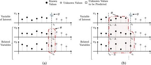
This approach is obviously sub-optimal, since at time $t_0$ the values of all the variables in Tables 2 and 3 are known for each of the measurement taken before $t_0$. For this reason, as depicted in Figure 5(b), it is possible to feed the model not just the variables of Table 2 at time $t_0$ but also all the measurements of these variables in $[t_0-\mathrm{\Delta },t_0]$, and the variables of Table 3 in $[t_0-\mathrm{\Delta },t_0]$ as an input. Thanks to this approach the authors are now able to map a time-series problem again into a classical multivariate regression problem (Packard et al. 1980; Takens 1981), and exploit the methods described in Sections 4.3 and 4.4. Note that Δ is an application specific parameter that needs to be tuned and its effect will be tested in Section 5. Note that, the methodology described in Sections 4.3 and 4.4 is a special case of what described in this section, and correspond to the case when $\mathrm{\Delta }=0$.

4.6. Feature ranking

Once the models are built it is required to investigate how these models are affected by the different features used in the model identification phase to understand if the models have also a foundation which relies on the underlying phenomena or if the model just captures spurious correlations (Guyon and Elisseeff 2003). This procedure is called Feature Ranking (FR) and allows to detect if the importance of those features, that are known to be relevant from a physical perspective, are appropriately taken into account by the learned models. The failure of the computational model to properly account for the relevant features might indicate poor quality in the measurements or spurious correlations. FR therefore represents an important step of model verification, since it should generate consistent results with the available knowledge of the phenomena under exam.

For this purpose, authors will adopt the backward elimination techniques described in Guyon and Elisseeff (2003). Note that, when $\mathrm{\Delta }=0$ (see Section 4.5) the feature ranking will be the classical one where the authors consider the variables of Tables 2 and 3 as features. When $\mathrm{\Delta }>0$ a new concept of feature ranking will be defined by the authors, where the entire time-series of the variables of Tables 2 and 3 will be considered as features.

5. Experimental results

In this section, the authors utilise the data described in Section 3 to test the models developed in Section 4, using the performance measures described in Section 4.1. To begin with, calibration results of the PM described in Section 4.2 are reported. Subsequently, the validation of the PM is carried out, both in steady and dynamic state as reported in Section 5.1. Then a comparison of the performance of PMs, DDMs, and HMs in operational conditions is reported in Section 5.2.

5.1. PM validation

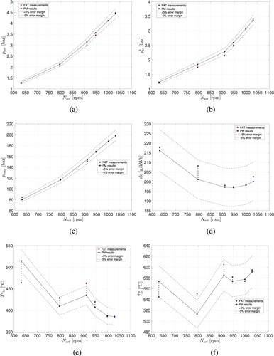
In line with the standard academic and industrial procedure (Theotokatos and Tzelepis 2015), the PM has been calibrated with data provided by the manufacturer, namely the FAT protocol. The percentage error (PE) between the measured values during the engine shop trials, and the predicted values by the PM, is reported in Table 4.

Table 4. PM FAT validation results.

Speed (rpm)	FAT (bar)	PM (bar)	PE (%)
Charge air pressure – $p_{\mathrm{a}\mathrm{i}\mathrm{r}}$
631	1.250	1.287	2.988
795	2.050	2.122	3.535
910	2.980	3.141	5.409
947	3.450	3.560	3.192
1000	4.120	4.117	-0.071
1031	4.480	4.442	-0.850
Relative exhaust gas receiver pressure – $p_{\mathrm{t}\mathrm{c}}^b$
631	1.205	1.228	1.947
795	1.741	1.842	5.814
910	2.140	2.286	6.811
947	2.490	2.591	4.065
1000	3.060	3.060	-0.004
1031	3.420	3.371	-1.429
Relative maximum combustion pressure – $p_{\mathrm{m}\mathrm{a}\mathrm{x}}$
631	85.000	80.309	−5.519
795	118.000	116.632	−1.159
910	151.000	154.260	2.159
947	168.000	169.063	0.633
1000	188.000	187.949	−0.027
1031	198.000	198.853	0.431
Specific fuel oil consumption – $\mathrm{s}\mathrm{f}\mathrm{c}$
Speed (rpm)	FAT (g/kWh)	PM (g/kWh)	PE (%)
631	217.9	216.278	−0.745
795	208.2	201.181	−3.371
910	198.1	197.224	−0.442
947	197.4	196.983	−0.211
1000	198.3	198.207	−0.047
1031	202.7	200.162	−1.252
Mean exhaust gas temperature after turbine – ${\overline{T}}_{\mathrm{t}\mathrm{c}}^a$
Speed (rpm)	FAT (${}^{\circ }$C)	PM (${}^{\circ }$C)	PE (%)
631	545.0	574.039	5.328
795	551.0	513.319	−6.839
910	605.0	585.022	−3.302
947	582.0	573.862	−1.398
1000	574.0	577.620	0.631
1031	595.0	591.461	−0.595
Mean exhaust gas temperature before turbine – ${\overline{T}}_{\mathrm{t}\mathrm{c}}^b$
Speed (rpm)	FAT (${}^{\circ }$C)	PM (${}^{\circ }$C)	PE (%)
631	464.0	514.5	9.916
795	429.0	409.4	−4.524
910	463.0	434.6	−6.090
947	420.0	407.5	−2.929
1000	386.0	387.5	0.433
1031	386.0	385.2	−0.147

The PM achieved predictions of sufficient accuracy for the entire speed range. The observed PEs are always lower than 10%, also considering the mean exhaust gas temperature after and before the turbine. Nevertheless, very high accuracy (less than 1%) is obtained at the MCR speed, this is attributed to the fact that the model hyperparameters were tuned specifically for this point and therefore, deviations of the PM performance are expected for the lower engine speed region. However, the PM predictions are satisfactory and the model can be used for the scope of this work.

Results of the calibration are reported in Figure 6, from which it can be seen that the PM achieves a mean PE of ±5% for all parameters reported, apart from the mean exhaust gas temperature before and after turbine. These results are in agreement with the relevant available literature (Guan et al. 2015; Theotokatos and Tzelepis 2015; Sui et al. 2017). After the calibration phase, the PM validation was performed according to the discussion of Section 4.2, at different DE speeds and loads, to assess model performance with respect to exhaust gas temperatures on the real world data described in Section 3, considering steady-state and dynamic conditions separately.

Figure 6. PM FAT validation results: (a) charge air pressure, (b) relative exhaust gas receiver pressure, (c) relative maximum combustion pressure, (d) specific fuel oil consumption, (e) mean exhaust gas temperature after turbine, (f) mean exhaust gas temperature before turbine.

The results of the steady-state simulations are reported in Figure 8 and Table 5, while the results of the dynamic operating conditions are reported in Figure 9 and Table 6. From Tables 5 and 6, it can be observed that for ${\overline{T}}_{\mathrm{t}\mathrm{c}}^a$ the MAPE is significantly greater than 10% and significantly higher than the MAPE for the FAT data points. For example, for ${\overline{T}}_{\mathrm{t}\mathrm{c}}^b$, the MAPE observed is greater than 20%. This is caused by running the engine at different operating points than the operating points at which the model was calibrated. For calibration, the FAT operating points were used, all on the theoretical propeller curve and above 650 rpm engine speed, while Figure 7 demonstrates that in static and dynamic operating conditions, the engine is running at speeds below 650 rpm and the control system forces the engine to run at loads below the theoretical propeller curve. The FAT measurement at 650 rpm already showed an error of +10% for temperature prediction, while the results in Figures 7 and 8 demonstrate that the greatest prediction errors are below 700 rpm and between 150 and 350${}^{\circ }$C and appear to get worse with further reducing loads and speeds. These large errors are clearly caused by the fact that the model was not calibrated for low speeds and low powers and by the modelling assumptions. Furthermore, the results in Figures 7(a) and 8(b) also illustrate the two different control modes with two different combinator curves that lead to two distinct areas in the scatter plots.

Figure 7. PM steady state operating conditions: (a) engine power and speed, (b) mean exhaust gas temperature before turbine.

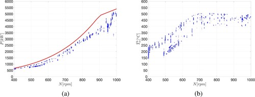
Figure 8. PM steady-state operating condition: (a) mean exhaust gas temperature after turbine and (b) mean exhaust gas temperature before turbine.

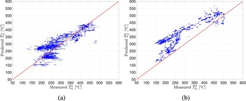
Figure 9. PM dynamic operating condition: (a) mean exhaust gas temperature after turbine and (b) mean exhaust gas temperature before turbine.

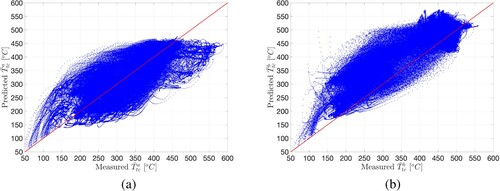
Table 5. PM steady-state performance measures.

Symbol	MAE (${}^{\circ }$C)	MAPE (%)	PPMCC
$T_{\mathrm{t}\mathrm{c}}^a$	38.4	15.8	0.85
$T_{\mathrm{t}\mathrm{c}}^b$	74.9	33.2	0.87

Table 6. PM Dynamic operating conditions performance measures.

Symbol	MAE (${}^{\circ }$C)	MAPE (%)	PPMCC
$T_{\mathrm{t}\mathrm{c}}^a$	33	10.9	0.86
$T_{\mathrm{t}\mathrm{c}}^b$	64	22.1	0.89

Moreover, comparing the results from Tables 5 and 6 with the scatter plots reported in Figures 8 and 9, interesting observations can be made that cannot be established from the MAPE. While the prediction of the temperature in static conditions appears to be fairly consistent, and could possibly be predicted more accurately with more accurate assumptions, higher order dynamics appear to have a great effect on temperature prediction that cannot be captured by the PM. In particular, the model's predictions of ${\overline{T}}_{\mathrm{t}\mathrm{c}}^a$ are acting as a low-pass filter. In conclusion, the PM in this case is first characterised by highly biased predictions, as reported in the scatter plots of Figures 8 and 9, and second is acting as a low-pass filter for dynamic operations. This indicates that the Seiliger cycle module (module D in Figure 4) needs to be improved to accurately capture operation over the complete operating profile and presents limitations in dynamic operating conditions.

5.2. Models performance comparison

In this section, the authors will compare the performance of PMs, DDMs, and HMs, described in Section 4, in operational conditions using the data described in Section 3.

In order to build ${\mathcal{D}}_n$ and ${\mathcal{T}}_m$, the authors split the data in different temporal slots in such a way that data belonging to ${\mathcal{D}}_n$ corresponds to a different temporal slot with respect to ${\mathcal{T}}_m$. The two data sets consist of various different manoeuvres using the two control modes described in Geertsma, Negenborn, Visser and Hopman (2017):

• Manoeuvre Mode (MM): combinator curve with relative low pitch, high engine speed and fast acceleration rates;

• Transit Mode (TM): combinator curve with higher pitch, lower engine speed and slow acceleration rates.

The error metrics reported in Tables 8 and 9, refer to ${\mathcal{T}}_m$. Figures 10–14 have been included purely for illustrative purposes, and correspond to a subset of ${\mathcal{T}}_m$, which covers 24 h of continuous operation of the DE in a healthy mix of steady-state and dynamic conditions, as described in Table 7.

Figure 10. Scatter plot (measured vs predicted) and trend in time for ${\overline{T}}_{\mathrm{t}\mathrm{c}}^a$ using a PM with $\mathrm{\Delta }=0$.

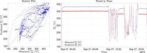
Table 7. Testing dataset operational description – illustrative subset.

Time (h)	Mode	Revolutions (rpm)	Engine load (%)
13	TM	760	50 to 55
3	MM	various speeds up to 850	various load from idle to 50
2	TM	780	55 to 60
$1\frac{3}{4}$	MM	low 500 to 600	up to 20
$1\frac{1}{2}$	TM	400 to 550	low Load
$\frac{1}{4}$	TM	increasing from 400 to 780	increasing from 10 to 60
$2\frac{1}{2}$	TM	780	55 to 60

Table 8. Indexes of performances (MAE, MAPE, and PPMCC) of the different models (PMs, DDMs, and HMs) for different $\mathrm{\Delta }\in \{0,10,20,30\}$ for ${\overline{T}}_{\mathrm{t}\mathrm{c}}^a$. Note that $\mathrm{\Delta }=0$ means that the authors do not exploit time series information from the past, for $\mathrm{\Delta }>0$ there is no PM result as described in Section 4.

Δ	Model	MAE (${}^{\circ }$C)	MAPE ($\text{\%}$)	PPMCC
0	PM	$33.0\pm 1.7$	$11.7\pm 0.5$	$0.86\pm 0.05$
	DDM	$7.9\pm 0.4$	$2.1\pm 0.1$	$0.99\pm 0.05$
	HM	$5.6\pm 0.3$	$1.5\pm 0.1$	$0.99\pm 0.05$
10	DDM	$10.3\pm 0.5$	$2.7\pm 0.1$	$0.98\pm 0.05$
	HM	$8.8\pm 0.4$	$2.3\pm 0.1$	$0.98\pm 0.05$
20	DDM	$4.8\pm 0.2$	$1.3\pm 0.1$	$1.00\pm 0.05$
	HM	$2.4\pm 0.1$	$0.6\pm 0.1$	$1.00\pm 0.05$
30	DDM	$12.7\pm 0.6$	$3.3\pm 0.2$	$0.97\pm 0.05$
	HM	$12.0\pm 0.5$	$3.1\pm 0.1$	$0.97\pm 0.04$

Table 9. Indexes of performances (MAE, MAPE and PPMCC) of the different models (PMs, DDMs, and HMs) for different $\mathrm{\Delta }\in \{10,20,30\}$ for ${\overline{T}}_{\mathrm{t}\mathrm{c}}^b$. Note that $\mathrm{\Delta }=0$ means that the authors do not exploit time series information from the past, for $\mathrm{\Delta }>0$ there is no PM result as described in Section 4.

Δ	Model	MAE (${}^{\circ }$C)	MAPE ($\text{\%}$)	PPMCC
0	PM	$64.2\pm 1.2$	$22.3\pm 0.4$	$0.89\pm 0.05$
	DDM	$8.8\pm 0.4$	$2.3\pm 0.1$	$0.98\pm 0.04$
	HM	$6.4\pm 0.4$	$1.7\pm 0.1$	$0.99\pm 0.06$
10	DDM	$11.1\pm 0.5$	$2.9\pm 0.1$	$0.98\pm 0.05$
	HM	$9.6\pm 0.5$	$2.5\pm 0.1$	$0.98\pm 0.05$
20	DDM	$5.6\pm 0.3$	$1.5\pm 0.1$	$0.99\pm 0.06$
	HM	$3.2\pm 0.2$	$0.8\pm 0.1$	$1.00\pm 0.05$
30	DDM	$13.5\pm 0.6$	$3.5\pm 0.1$	$0.96\pm 0.04$
	HM	$12.8\pm 0.6$	$3.3\pm 0.2$	$0.97\pm 0.05$

As reported in Section 4.2, PMs are limited to only handling the case with $\mathrm{\Delta }=0$. More precisely, $\mathrm{\Delta }>0$ does not improve the model. When it comes to the DDMs, the custom algorithm described in Section 4.3 will be exploited. The set of hyperparameters tuned during the MS phase are $\mathcal{H}=\{\gamma ,\lambda \}$ chosen in $\mathfrak{H}=\{{10}^{-4.0},{10}^{-3.8},\dots ,{10}^{+4.0}\}\times \{{10}^{-4.0},{10}^{-3.8},\dots ,{10}^{+4.0}\}$.

Eventually, the HMs custom algorithm described in Section 4.4 will be exploited. The set of hyperparameters tuned during the MS phase are $\mathcal{H}=\{\gamma ,\lambda ,\theta \}$ chosen in $\mathfrak{H}=\{{10}^{-4.0},{10}^{-3.8},\dots ,{10}^{+4.0}\}\times \{{10}^{-4.0},{10}^{-3.8},\dots ,{10}^{+4.0}\}$ $\times \{{10}^{-4.0},{10}^{-3.8},\dots ,{10}^{+4.0}\}$.

All the tests have been repeated 30 times, and the average results are reported together with their t-student $95\text{\%}$ confidence interval, to ensure the statistical validity of the results.

5.2.1. PM results

As indicated by the error metrics of Tables 8 and 9, the PM does not predict the exhaust gas temperatures at turbine inlet (${\overline{T}}_{\mathrm{t}\mathrm{c}}^b$) and outlet (${\overline{T}}_{\mathrm{t}\mathrm{c}}^a$) to a satisfactory degree, regardless of the operating (steady-state or dynamic) conditions. As shown in Table 5 and Figure 8, the PM is characterised by low bias and high variance in predicting ${\overline{T}}_{\mathrm{t}\mathrm{c}}^a$, and by high bias and high variance in predicting ${\overline{T}}_{\mathrm{t}\mathrm{c}}^b$. The same applies to dynamic conditions, according to Table 6, and Figure 9. For the sake of clarity, a representative time-series sample of the PMs' predictions is reported in Figure 10 for $\overline{T_{\mathrm{t}\mathrm{c}}^a}$.

On one hand, these discrepancies can be attributed to the following assumptions and simplifications (Geertsma, Negenborn, Visser, Loonstijn, et al. 2017):

• Pressure losses in the inlet duct, filter and air cooler are neglected.

• Heat transfer effects along the air and exhaust-gas paths are neglected, namely, heat losses in the inlet duct, filter and intercooler.

• Regarding the combustion process, the constant volume portion of combustion increases linearly with engine speed, and the temperature portion of combustion increases proportionately to fuel injection.

• Fuel injection time delay is constant.

• Scavenge efficiency is constant and equal to unity.

• Heat loss modelling during the expansion and blowdown processes has been simplified.

• Namely, the heat release efficiency is inversely related to engine speed.

• Air temperature at the start of compression is constant.

• Combustion efficiency is constant.

• The expansion in the turbine is polytropic.

• The polytropic efficiency between compressor and turbine has been split equally.

• Turbine efficiency is a quadratic function with respect to charge pressure.

• Air and exhaust gas properties have been kept constant throughout.

• The lower heating value of the fuel is equal to 42,700 [kJ/kg], according to ISO standards.

The model calibration and more advanced assumptions could enable significant improvement to the PM, but only if sufficient calibration data is available over the complete engine operating envelop. On the other hand, the aforementioned assumptions and simplifications enabled the PM to reach a good trade-off between accuracy (in steady-state) and computational time, making the model's run-time close to 2500 times real-time, much faster than MVEMs characterised by the presence of the compressor and turbine maps (Theotokatos and Tzelepis 2015; Sapra et al. 2017). For the reasons discussed above, although the PM is suitable for real-time applications, its accuracy is not sufficient for accurate temperature prediction in dynamic conditions that allows early identification of emerging failures.

5.2.2. DDMs results

The proposed DDMs are more accurate in predicting both ${\overline{T}}_{\mathrm{t}\mathrm{c}}^a$ and ${\overline{T}}_{\mathrm{t}\mathrm{c}}^b$ compared to the PM, even without considering past information ($\mathrm{\Delta }>0$). Of course, when this information is also taken into account, the error metrics drop by around 50% (e.g. MAPE reduces from $2.1\text{\%}\pm 0.5\text{\%}$ to $1.3\text{\%}\pm 0.1\text{\%}$) as reported in Tables 8 and 9. In Figures 11 and 13, representative time-series of the predictions of $\overline{T_{\mathrm{t}\mathrm{c}}^a}$ are shown.

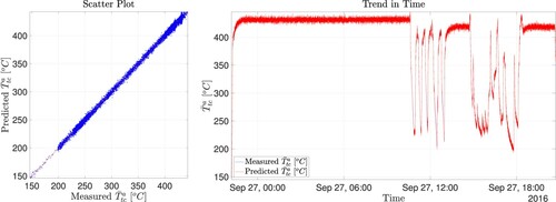
Figure 11. Scatter plot (measured vs predicted) and trend in time for ${\overline{T}}_{\mathrm{t}\mathrm{c}}^a$ using a DDM with $\mathrm{\Delta }=0$.

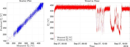
From Figures 11 and 13, it is possible to observe that DDMs are capable of fully capturing the thermodynamic transients of the exhaust gases, both in steady-state and dynamic conditions, as shown in Table 7. From Figures 11–13, it can be observed that the DDMs are characterised by both lower bias and lower variance, with respect to the PM. The optimal time window (Δ) is found for a value equal to 20 s. For this value, minimal error metrics among all DDMs occur. According to Table 8, for this time window, the MAPE for ${\overline{T}}_{\mathrm{t}\mathrm{c}}^b$ is as low as $1.3\text{\%}\pm 0.1\text{\%}$, whereas for ${\overline{T}}_{\mathrm{t}\mathrm{c}}^a$, the MAPE is $1.5\text{\%}\pm 0.1\text{\%}$, as reported in Table 9. Furthermore, from the scatter plot of Figure 13, it can be observed that minimum variance is also achieved.

It should be noted that, although DDMs are computationally demanding in the training phase, they are characterised by lower computational complexity in the feed-forward phase, as they just require matrix manipulation methods, in contrast with the solution of a system of DAEs that the PM requires. The combination of both accurate and fast predictions, makes DDMs an ideal candidate for real-time performance and condition estimation. However, the necessary data to reach this level of performance is rather high (Cipollini et al. 2018a, 2018b), which makes this type of models applicable only after extensive measurement campaigns have been undertaken. Finally, another disadvantage of DDMs is the lack of interpretability as it is not supported by any physical interpretation (Shawe-Taylor and Cristianini 2004).

5.2.3. HMs Results

To overcome the limitations discussed in Sections 5.2.1 and 5.2.2 for the PMs and DDMs, respectively, the authors have proposed the use of HMs. These allow the exploitation of both the mechanistic knowledge of the underlying physical principles from the PM, and any available measurements taken during the operation of the vessel.

The novelty introduced by the HMs led to more accurate predictions of both ${\overline{T}}_{\mathrm{t}\mathrm{c}}^a$ and ${\overline{T}}_{\mathrm{t}\mathrm{c}}^b$ compared to the rest of the models, regardless of the time window considered (Δ), as can be seen from Tables 8 and 9. Furthermore, the same tables reveal that the optimal model is an HM with a time window of 20 s, which achieves MAPEs of $0.6\text{\%}\pm 0.1\text{\%}$ for ${\overline{T}}_{\mathrm{t}\mathrm{c}}^b$, and $0.8\text{\%}\pm 0.1\text{\%}$ for ${\overline{T}}_{\mathrm{t}\mathrm{c}}^a$. This is also supported by Figures 12 and 14, which show representative time-series of the predictions of ${\overline{T}}_{\mathrm{t}\mathrm{c}}^a$ for time windows of 10 and 20 s, respectively. It can be seen that the variance has been completely eliminated, whereas the bias has been reduced to near-zero levels.

Figure 12. Scatter plot (measured vs predicted) and trend in time for ${\overline{T}}_{\mathrm{t}\mathrm{c}}^a$ using an HM with $\mathrm{\Delta }=0$.

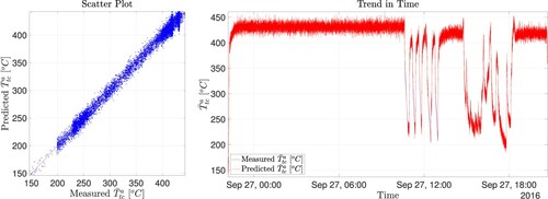
Figure 13. Scatter plot (measured vs predicted) and trend in time for ${\overline{T}}_{\mathrm{t}\mathrm{c}}^a$ using a DDM with $\mathrm{\Delta }=20$ which is the best one as shown in Table 9.

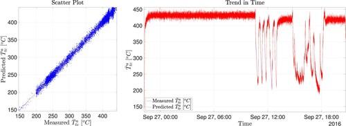
Figure 14. Scatter plot (measured vs predicted) and trend in time for ${\overline{T}}_{\mathrm{t}\mathrm{c}}^a$ using an HM with $\mathrm{\Delta }=20$ which is the best one as shown in Table 9.

An advantage of the HMs is their ability to exploit the coarse, but physically supported, predictions of the PM. Therefore, they have much smaller requirements regarding the use of actual measurements for the learning phase (Coraddu et al. 2017). While they will still require a measurement campaign in order to be deployed, they can be reliably used already after a few months worth of measurements, in contrast with pure DDMs that would require at least half a year of available data, before they can be exploited.

5.2.4. Features ranking results

In Tables 10 and 11, the top ranked features are reported for the top performing models, namely the DDMs and HMs for every time window. Starting from $\mathrm{\Delta }=0$, it can be seen that the DDM model ranks the relevant features consistently with respect to engineering knowledge. As expected, the high-temperature (HT) and low-temperature (LT) cooling water temperatures after the coolers ($T_{\mathrm{h}\mathrm{t}}^a$, $T_{\mathrm{l}\mathrm{t}}^a$), in combination with the temperatures for main bearing 4 and 5 ($T_{b_4}$, $T_{b_5}$), have the highest predictive power for ${\overline{T}}_{\mathrm{t}\mathrm{c}}^a$, according to Table 10. This is to be expected because both the lube oil system (where bearings 4 and 5 carry the highest load) and the cooling water system absorb the largest part of the overall heat rejection of the engine, which is tightly coupled with the power output of the engine and serves as an overall indicator for the average temperature increase at each of the measurement points as shown in Figure 3. Moreover, the charge air temperature after compressor (Bank A – Column 6) $T_{cA}^a$, the charge air temperature before turbine (Bank B – Column 8) $T_{cB}^a$, and the turbine speed $N_{{\mathrm{t}\mathrm{c}}_B}$ (Bank B – Column 7) have influence on the prediction. It should be noted that to compare the real measurements from the IPMS with the PM outcomes, the authors considered the average value of the Banks A and B. For this reason, in Table 10, Bank A and Bank B contribution cannot be captured independently by the DDMs and HMs. The same conclusion can be drawn from Table 11.

Table 10. Top 10 feature in $\mathcal{X}$, ranked in descending importance, of the different models (DDMs and HMs) for different $\mathrm{\Delta }\in \{0,10,20,30\}$ for ${\overline{T}}_{\mathrm{t}\mathrm{c}}^a$. Note that, for $\mathrm{\Delta }>0$, the importance does not refer to the single feature in $\mathcal{X}$ but the entire past temporal series.

		Ranked position
Δ	Model	1	2	3	4	5	6	7	8	9	10
0	DDM	$T_{\mathrm{h}\mathrm{t}}^a$	$T_{\mathrm{l}\mathrm{t}}^a$	$T_{\mathrm{a}\mathrm{i}\mathrm{r}}$	$T{a}_{{\mathrm{t}\mathrm{c}}_A}^b$	$T_{\mathrm{l}\mathrm{o}}^b$	$T_{c_A}^a$	$N_{{\mathrm{t}\mathrm{c}}_B}$	$T{a}_{{\mathrm{t}\mathrm{c}}_B}^b$	$P_m^{\mathrm{m}\mathrm{a}\mathrm{x}}$	$T_{b_5}$
	HM	${\overline{T}}_{\mathrm{t}\mathrm{c}}^a$ (PM)	$T_{\mathrm{a}\mathrm{i}\mathrm{r}}$	$P_m^{\mathrm{m}\mathrm{a}\mathrm{x}}$	$T_{b_4}$	$p_{\mathrm{a}\mathrm{i}\mathrm{r}}$	$T{a}_{{\mathrm{t}\mathrm{c}}_B}^b$	$T_{{\mathrm{s}\mathrm{o}}_4}$	$T_{b_7}$	$T_{{\mathrm{s}\mathrm{o}}_2}$	$N_{{\mathrm{t}\mathrm{c}}_B}$
10	DDM	${\overline{T}}_{\mathrm{t}\mathrm{c}}^a$	$T_{\mathrm{l}\mathrm{t}}^b$	$T{a}_{{\mathrm{t}\mathrm{c}}_B}^b$	$T_{c_A}^a$	$T_{b_4}$	$T_{b_3}$	$T_{b_5}$	$T_{{\mathrm{s}\mathrm{o}}_4}$	$T_{\mathrm{h}\mathrm{t}}^b$	$T_{{\mathrm{s}\mathrm{o}}_2}$
	HM	${\overline{T}}_{\mathrm{t}\mathrm{c}}^a$	${\overline{T}}_{\mathrm{t}\mathrm{c}}^a$ (PM)	$T_{b_3}$	$T_{\mathrm{a}\mathrm{i}\mathrm{r}}$	$p_{\mathrm{a}\mathrm{i}\mathrm{r}}$	$T_{\mathrm{h}\mathrm{t}}^b$	$T_{\mathrm{l}\mathrm{t}}^a$	$T_{c_A}^a$	$T{a}_{{\mathrm{t}\mathrm{c}}_B}^b$	$T_{\mathrm{h}\mathrm{t}}^a$
20	DDM	${\overline{T}}_{\mathrm{t}\mathrm{c}}^a$	$T{a}_{{\mathrm{t}\mathrm{c}}_B}^b$	$T{a}_{{\mathrm{t}\mathrm{c}}_A}^b$	$T_{b_3}$	$T_{b_4}$	$T_{\mathrm{h}\mathrm{t}}^a$	$T_{\mathrm{l}\mathrm{t}}^b$	$p_{\mathrm{a}\mathrm{i}\mathrm{r}}$	$T_{\mathrm{l}\mathrm{o}}^b$	$T_{\mathrm{a}\mathrm{i}\mathrm{r}}$
	HM	${\overline{T}}_{\mathrm{t}\mathrm{c}}^a$	${\overline{T}}_{\mathrm{t}\mathrm{c}}^a$ (PM)	$T{a}_{{\mathrm{t}\mathrm{c}}_B}^b$	$T_{c_A}^a$	$T_{\mathrm{h}\mathrm{t}}^b$	$T_{b_4}$	$T_{b_3}$	$p_{\mathrm{a}\mathrm{i}\mathrm{r}}$	$T_{{\mathrm{s}\mathrm{o}}_2}$	$P_m^{\mathrm{m}\mathrm{a}\mathrm{x}}$
30	DDM	${\overline{T}}_{\mathrm{t}\mathrm{c}}^a$	$T{a}_{{\mathrm{t}\mathrm{c}}_B}^b$	$T_{\mathrm{h}\mathrm{t}}^b$	$T_{{\mathrm{s}\mathrm{o}}_4}$	$P_m^{\mathrm{m}\mathrm{a}\mathrm{x}}$	$T_{b_7}$	$T_{\mathrm{h}\mathrm{t}}^a$	$T_{c_A}^a$	$p_{\mathrm{a}\mathrm{i}\mathrm{r}}$	$T_{{\mathrm{s}\mathrm{o}}_2}$
	HM	${\overline{T}}_{\mathrm{t}\mathrm{c}}^a$	${\overline{T}}_{\mathrm{t}\mathrm{c}}^a$ (PM)	$T_{\mathrm{h}\mathrm{t}}^a$	$T_{b_7}$	$T_{\mathrm{l}\mathrm{o}}^b$	$T{a}_{{\mathrm{t}\mathrm{c}}_A}^b$	$T_{b_3}$	$p_{\mathrm{a}\mathrm{i}\mathrm{r}}$	$N_{{\mathrm{t}\mathrm{c}}_B}$	$P_m^{\mathrm{m}\mathrm{a}\mathrm{x}}$

Table 11. Top 10 feature in $\mathcal{X}$, ranked in descending importance, of the different models (DDMs and HMs) for different $\mathrm{\Delta }\in \{0,10,20,30\}$ for ${\overline{T}}_{\mathrm{t}\mathrm{c}}^b$. Note that, for $\mathrm{\Delta }>0$, the importance does not refer to the single feature in $\mathcal{X}$ but the entire past temporal series.

		Ranked position
Δ	Model	1	2	3	4	5	6	7	8	9	10
0	DDM	$T_{b_4}$	$T_{b_5}$	$T_{\mathrm{h}\mathrm{t}}^a$	$T_{\mathrm{a}\mathrm{i}\mathrm{r}}$	$T{a}_{{\mathrm{t}\mathrm{c}}_B}^b$	$T_{c_A}^a$	$T{a}_{{\mathrm{t}\mathrm{c}}_A}^b$	$n_{\mathrm{a}\mathrm{c}\mathrm{t}}$	$P_m^{\mathrm{m}\mathrm{a}\mathrm{x}}$	$N_{{\mathrm{t}\mathrm{c}}_B}$
	HM	${\overline{T}}_{\mathrm{t}\mathrm{c}}^b$ (PM)	$T_{c_A}^a$	$N_{{\mathrm{t}\mathrm{c}}_B}$	$T_{b_6}$	$T_{b_4}$	$T_{b_3}$	$T_{\mathrm{h}\mathrm{t}}^b$	$n_{\mathrm{a}\mathrm{c}\mathrm{t}}$	$T_{\mathrm{l}\mathrm{o}}^a$	$T_{\mathrm{h}\mathrm{t}}^a$
10	DDM	${\overline{T}}_{\mathrm{t}\mathrm{c}}^b$	$T_{c_A}^a$	$T_{\mathrm{a}\mathrm{i}\mathrm{r}}$	$T_{b_6}$	$T_{b_7}$	$T_{\mathrm{h}\mathrm{t}}^a$	$P_m^{\mathrm{m}\mathrm{a}\mathrm{x}}$	$T{a}_{{\mathrm{t}\mathrm{c}}_B}^b$	$m_f$	$T_{b_4}$
	HM	${\overline{T}}_{\mathrm{t}\mathrm{c}}^b$	${\overline{T}}_{\mathrm{t}\mathrm{c}}^b$ (PM)	$T_{b_6}$	$T_{\mathrm{h}\mathrm{t}}^a$	$T_{b_3}$	$P_m^{\mathrm{m}\mathrm{a}\mathrm{x}}$	$T_{b_4}$	$T_{b_5}$	$m_f$	$T_{b_7}$
20	DDM	${\overline{T}}_{\mathrm{t}\mathrm{c}}^b$	$T_{\mathrm{h}\mathrm{t}}^a$	$p_{\mathrm{a}\mathrm{i}\mathrm{r}}$	$T_{\mathrm{l}\mathrm{o}}^a$	$T_{b_7}$	$T_{c_A}^a$	$T_{\mathrm{h}\mathrm{t}}^b$	$T_{b_4}$	$T_{b_3}$	$m_f$
	HM	${\overline{T}}_{\mathrm{t}\mathrm{c}}^b$	${\overline{T}}_{\mathrm{t}\mathrm{c}}^b$ (PM)	$m_f$	$T_{b_5}$	$T{a}_{{\mathrm{t}\mathrm{c}}_A}^b$	$T_{b_4}$	$N_{{\mathrm{t}\mathrm{c}}_B}$	$T_{b_7}$	$T_{\mathrm{h}\mathrm{t}}^b$	$T_{\mathrm{h}\mathrm{t}}^a$
30	DDM	${\overline{T}}_{\mathrm{t}\mathrm{c}}^b$	$T_{\mathrm{a}\mathrm{i}\mathrm{r}}$	$m_f$	$T_{b_5}$	$T{a}_{{\mathrm{t}\mathrm{c}}_B}^b$	$P_m^{\mathrm{m}\mathrm{a}\mathrm{x}}$	$T_{b_4}$	$T_{\mathrm{l}\mathrm{t}}^a$	$T{a}_{{\mathrm{t}\mathrm{c}}_A}^b$	$T_{b_3}$
	HM	${\overline{T}}_{\mathrm{t}\mathrm{c}}^b$	${\overline{T}}_{\mathrm{t}\mathrm{c}}^b$ (PM)	$T_{b_3}$	$T{a}_{{\mathrm{t}\mathrm{c}}_A}^b$	$T_{b_4}$	$T_{c_A}^a$	$T_{\mathrm{h}\mathrm{t}}^b$	$T_{b_7}$	$T_{\mathrm{h}\mathrm{t}}^a$	$P_m^{\mathrm{m}\mathrm{a}\mathrm{x}}$

Considering the HM's feature ranks from Table 10, it should be highlighted that they use as inputs ${\overline{T}}_{\mathrm{t}\mathrm{c}}^a$ and ${\overline{T}}_{\mathrm{t}\mathrm{c}}^a$ from the PM. Highest predictive power is observed for ${\overline{T}}_{\mathrm{t}\mathrm{c}}^a\left(PM\right)$, a result that acts as a sanity check on the feature ranking procedure's robustness. The same features discussed for the DDMs are the most important ones also for the HMs. Nevertheless, non-linear correlations between the different features lead to a slight variation in the features' position. When time windows are also employed (models with $\mathrm{\Delta }>0$), the most important feature for the prediction of each temperature, as expected, is the time-history of the temperature itself as reported in Sections 5.2.3 and 5.2.4, and depicted in Figure 5(b).

It can be noted that the models rank approximately the same features among the different time windows. From a physical point of view, this can be considered as a sanity check for the reliability and robustness of the model.

6. Conclusion and discussion

In this work, the authors developed novel hybrid approaches to model diesel engine exhaust gas temperatures in operational conditions. With this purpose in mind, a hybrid modelling approach is introduced, to build a robust and reliable diesel engine model suitable for real-time performance assessment and condition monitoring applications. A state-of-the-art Kernel method has been presented, able to exploit the information provided by on-board measurements from one Holland Class Oceangoing Patrol Vessel, provided by the Royal Netherlands Navy and Damen Schelde Naval Shipbuilding.

To define the improvements brought by the proposed methodology, the authors first applied the standard approach used by industry experts and academics, by using and evaluating a first-principle-equation-based diesel engine model that is capable of providing real-time predictions. However, results in Section 5 show the following: while the calibration results indicated an adequate model that can capture the behaviour of the engine within 10% when using data from the factory acceptance test at operating points on the theoretical propeller curve, validation with real measurements revealed that the performance of the model over the true operating envelope is much worse. This greater error, up to 30% MAPE, is caused by running the engine at much lower loads and speeds, and due to the control strategy that forces the engine to other operating points than the theoretical propeller curve.

On the other hand, the data-driven models proposed in Section 4.3, are adequate in predicting the behaviour of the diesel engine, with a focus on exhaust gas temperatures. Classically, these exhaust gas temperatures would be approached by first principle thermodynamic and heat transfer equations, requiring very detailed design information and possibly lab scale tests to experimentally determine principle heat transfer coefficients. However, due to their nature, these data-driven models are hard to interpret.

To overcome the limitations of both the physical and the data-driven models, the authors developed a hybrid approach that can take into consideration past information, are capable of improving accuracy, are easily interpreted, and have low computational time requirements. These hybrid models can improve average errors by a factor 2 over purely data-driven models. These hybrid models can potentially also be used to improve accuracy of predictions for operation in other conditions than the measured ones, as purely data-driven models cannot be used for extrapolation, but the physical model contribution will improve hybrid model performance during extrapolation. While the hybrid approach will still require a measurement campaign in order to be deployed, this approach can be reliably used based on a significantly smaller dataset in comparison with the pure DDMs, for the same average error, as shown in Section 5.2.3. Moreover, the proposed methodology can also be applied to other industries facing problems of similar nature. Automotive, aviation, railway and process industries are potential candidates for the application of these types of models.

Next steps of the research will consider the utilisation of a more extensive data set containing engines of different vessels, the application of the proposed method to other systems installed on-board, and more importantly the application of the methodology for early fault detection and isolation.

Acknowledgments

This project is supported by the Royal Netherlands Navy supplying the operational measurement data from one Holland Class Oceangoing Patrol Vessel and Damen Schelde Naval Shipbuilding. The Royal Netherlands Navy supplied Figure 1 and maintains its copyright.

Disclosure statement

No potential conflict of interest was reported by the author(s).

References

- Al-Hinti I, Samhouri M, Al-Ghandoor A, Sakhrieh A. 2009. The effect of boost pressure on the performance characteristics of a diesel engine: A neuro-fuzzy approach. Appl Energy. 86:113–121.
- Amma NR. 2019. An environmental and economic analysis of methanol fuel for a cellular container ship. Trans Res D. 69:66–76.
- Anderson M, Salo K, Fridell E. 2015. Particle and gaseous emissions form an LNG powered ship. Environ Sci Technol. 49:12568–12575.
- Antonić R, Vukić Z, Kuljača O. 2004. Neuro-fuzzy modelling of marine diesel engine cylinder dynamics. IFAC Proc Vol. 37:95–100.
- Argyriou A, Evgeniou T, Pontil M. 2008. Convex multi-task feature learning. Mach Learn. 73:243–272.
- Asad U, Zheng M. 2014. Exhaust gas recirculation for advanced diesel combustion cycles. Appl Energy. 123:242–52.
- Bakker B, Heskes T. 2003. Task clustering and gating for Bayesian multitask learning. J Mach Learn Res. 4:83–99.
- Baldi F, Theotokatos G, Andersson K. 2015. Development of a combined mean value-zero dimensional model and application for a large marine four-stroke diesel engine simulation. Appl Energy. 154:402–415.
- Baldini A, Ciabattoni L, Felicetti R, Ferracuti F, Freddi A, Monteriú A. 2018. Dynamic surface fault tolerant control for underwater remotely operated vehicles. ISA Trans. 78:10–20.Advanced Methods in Control and Signal Processing for Complex Marine Systems.
- Banda OAV, Kannos S, Goerlandt F, van Gelder PH, Bergström M, Kujala P. 2019. A systemic hazard analysis and management process for the concept design phase of an autonomous vessel. Reliab Eng Syst Safety. 191:106584.
- Basurko OC, Uriondo Z. 2015. Condition-based maintenance for medium speed diesel engines used in vessels in operation. Appl Therm Eng. 80:404–412.
- Baxter J. 2000. A model of inductive bias learning. J Artif Intell Res. 12:149–198.
- Bhatti G, Mohan H, Singh R. 2021. Towards the future of smart electric vehicles. Digital twin technology. Renew Sustain Energy Rev. 141:110801.
- Bondarenko O, Fukuda T. 2020. Development of a diesel engine's digital twin for predicting propulsion system dynamics. Energy. 196:117126.
- Bukovac O, Medica V, Mrzljak V. 2015. Steady state performances analysis of modern marine two-stroke low speed diesel engine using MLP neural network model. Brodogradnja. 66:57–70.
- Cai B, Sun X, Wang J, Yang C, Wang Z, Kong X, Liu Z, Liu Y. 2020. Fault detection and diagnostic method of diesel engine by combining rule-based algorithm and BNs/BPNNs. J Manuf Syst. 57:148–157.
- Caruana R. 1997. Multitask learning. Mach Learn. 28:41–75.
- Cipollini F, Oneto L, Coraddu A, Murphy AJ, Anguita D. 2018a. Condition-based maintenance of naval propulsion systems: data analysis with minimal feedback. Reliab Eng Syst Safety. 177:12–23.
- Cipollini F, Oneto L, Coraddu A, Murphy AJ, Anguita D. 2018b. Condition-based maintenance of naval propulsion systems with supervised data analysis. Ocean Eng. 149:268–278.
- Coraddu A, Kalikatzarakis M, Oneto L, Meijn GJ, Godjevac M, Geertsmad RD. 2018. Ship diesel engine performance modelling with combined physical and machine learning approach. International Naval Engineering Conference and Exhibition (INEC).
- Coraddu A, Oneto L, Baldi F, Anguita S. 2017. Vessels fuel consumption forecast and trim optimisation: a data analytics perspective. Ocean Eng. 130:351–370.
- Coraddu A, Oneto L, Ilardi D, Stoumpos S, Theotokatos G. 2021. Marine dual fuel engines monitoring in the wild through weakly supervised data analytics. Eng Appl Artif Intell. 100:104179.
- Cristianini N, Shawe-Taylor J. 2000. An introduction to support vector machines and other kernel-based learning methods. Cambridge University Press.
- Curley R. 2012. The complete history of ships and boats. Britannica Educational Publishing.
- Dixon SL. 1998. Fluid mechanics and thermodynamics of thermomachinery. Butterworth Heinemann.
- Efron B, Tibshirani RJ. 1994. An introduction to the bootstrap. CRC Press.
- Evgeniou T, Pontil M. 2004. Regularized multi-task learning. ACM SIGKDD International Conference on Knowledge Discovery and Data Mining.
- Fernández-Delgado M, Cernadas E, Barro S, Amorim D. 2014. Do we need hundreds of classifiers to solve real world classification problems? J Mach Learn Res. 15:3133–3181.
- Galindo J, Lujan JM, Serrano JR, Hernández L. 2005. Combustion simulation of turbocharger HSDI diesel engines during transient operation using neural networks. Appl Therm Eng. 25:877–898.
- Gao Y, Karimi M, Kudreyko AA, Song W. 2018. Spare optimistic based on improved ADMM and the minimum entropy de-convolution for the early weak fault diagnosis of bearings in marine systems. ISA Trans. 78:98–104. Advanced Methods in Control and Signal Processing for Complex Marine Systems.
- Geertsma RD, Badon Ghijben NA, Zwart OR. 2013. Fire fighting and damage control automation: enabling future crew reduction. Engine as a Weapon International Symposium.
- Geertsma RD, Negenborn RR, Visser K, Hopman JJ. 2017. Parallel control for hybrid propulsion of multifunction ships. IFAC Proc Vol. 50(1):2296–2303.
- Geertsma RD, Negenborn RR, Visser K, Loonstijn MA, Hopman JJ. 2017. Pitch control for ships with diesel mechanical and hybrid propulsion: modelling, validation and performance quantification. Appl Energy. 206:1609–1631.
- Geertsma RD, Visser K, Negenborn RR. 2018. Adaptive pitch control for ships with diesel mechanical and hybrid propulsion. Appl Energy. 228:2490–2509.
- Geng P, Mao H, Hang Y, Wei L, You K, Ju J, Chen T. 2017. Combustion characteristics and NOx emissions of a waste cooking oil biodiesel blend in a marine auxiliary diesel engine. Appl Therm Eng. 115:947–954.
- Ghaderi H. 2019. Autonomous technologies in short sea shipping: trends, feasibility and implications. Trans Rev. 39:152–173.
- Ghelardoni L, Ghio A, Anguita D. 2013. Energy load forecasting using empirical mode decomposition and support vector regression. IEEE Trans Smart Grid. 4:549–556.
- Grimmelius HT. 2003. Simulation models in marine engineering: from training to concept exploration. In COMPIT.
- Grimmelius H, Mesbahi E, Schulten P, Stapersma D. 2007. The use of diesel engine simulation models in ship propulsion plant design and operation. CIMAC International Council on Combustion Engines. p. 1–12.
- Grondin O, Stobart R, Chafouk H, Maquet J. 2004. Modelling the compression ignition engine for control: review and future trends. Technical Report SAE Technical Paper.
- Guan C, Theotokatos G, Chen H. 2015. Analysis of two stroke marine diesel engine operation including turbocharger cut-out by using a zero-dimensional model. Energies. 8:5738–5764.
- Guyon I, Elisseeff A. 2003. An introduction to variable and feature selection. J Mach Learn Res. 3:1157–1182.
- Hao C, Lu Z, Feng Y, Bai H, Wen M, Wang T. 2021. Optimization of fuel/air mixing and combustion process in a heavy-duty diesel engine using fuel split device. Appl Therm Eng. 186:116458.
- Hoang AT, Tran VD, Dong VH, Le AT. 2019. An experimental analysis on physical properties and spray characteristics of an ultrasound-assisted emulsion of ultra-low-sulphur diesel and jatropha-based biodiesel. J Mar Eng Technol.
- Horenberg SC, Melaet ACF. 2013. Uniting weapon and marine knowledge. In Engine as a Weapon International Symposium.
- Hountalas DT. 2000. Prediction of marine diesel engine performance under fault conditions. Appl Therm Eng. 20:1753–1783.
- IMO MARPOL. 2011. International convention for the prevention of pollution from ships (MARPOL) annex VI. Consolidated edition International Maritime Organisation.
- IMO MEPC 72. 2018. Initial strategy on greenhouse gas emissions reduction for ships. Technical Report International Maritime Organisation.
- Johnson K, Mollenhauer K, Tschoke H. 2010. Handbook of diesel engines. Springer Science & Business Media.
- Kalikatzarakis M, Geertsma RD, Boonen EJ, Visser K, Negenborn RR. 2018. Ship energy management for hybrid propulsion and power supply with shore charging. Appl Energy. 76:133–154.
- Karimi HR, Zhang H, Ding S. 2018. Advanced methods in control and signal processing for complex marine systems. ISA Trans. 78:1–2. Advanced Methods in Control and Signal Processing for Complex Marine Systems.
- Keerthi SS, Lin CJ. 2003. Asymptotic behaviors of support vector machines with Gaussian kernel. Neural Comput. 15:1667–1689.
- Khaled AB, Gaid MB, Pernet N, Simon D. 2014. Fast multi-core co-simulation of cyber-physical systems: application to internal combustion engines. Simul Model Pract Theory. 47:79–91.
- Kohavi R. 1995. A study of cross-validation and bootstrap for accuracy estimation and model selection. In International Joint Conference on Artificial Intelligence.
- Kökkülünk G, Parlak A, Erdam HH. 2016. Determination of performance degradation of a marine diesel engine by using curve based approach. Appl Therm Eng. 108:1136–1146.
- Korczewski Z. 2015. Exhaust gas temperature measurements in diagnostics of turbocharged marine internal combustion engines part I standard measurements. Polish Marit Res. 22:47–54.
- Korczewski Z. 2016. Exhaust gas temperature measurements in diagnostics of turbocharged marine internal combustion engines part II dynamic measurements. Polish Marit Res. 23:68–76.
- Larsen U, Pierobon L, Baldi F, Haglind F, Ivarsson A. 2015. Development of a model for the prediction of the fuel consumption and nitrogen oxides emission trade-off for large ships. Energy. 80:545–555.
- Leifsson L, Sævarsdóttir H, Sigurdhsson S, Vésteinsson A. 2008. Grey-box modeling of an ocean vessel for operational optimization. Simul Model Pract Theory. 16:923–932.
- Liu M, Fang S, Dong H, Xu C. 2020. Review of digital twin about concepts, technologies, and industrial applications. J Manuf Syst. 58:346–361.
- Liu C, Negenborn RR, Chu X, Zheng H. 2017. Predictive path following based on adaptive line-of-sight for underactuated autonomous surface vessels. J Mar Sci Technol. 23(3):483–494.
- Liu C, Negenborn RR, Chu X, Zheng H. 2019. Colregs-constrained real-time path planning for autonomous ships using modified artificial potential fields. J Navig. 72(3):588–608.
- Llamas X, Eriksson L. 2018. Control-oriented modeling of two-stroke diesel engines with exhaust gas recirculation for marine applications. Proc Inst Mech Eng M: J Eng Maritime Environ. 233:551–574. doi:https://doi.org/10.1177/1475090218768992
- Lloyd AC, Cackette TA. 2001. Diesel engines: environmental impact and control. J Air Waste Manage Assoc. 51:809–847.
- Miglianti F, Cipollini F, Oneto L, Tani G, Viviani M. 2019. Model scale cavitation noise spectra prediction: combining physical knowledge with data science. Ocean Eng. 178:185–203.
- Namigtle-Jiménez A, Escobar-Jiménez R, Gómez-Aguilar J, García-Beltrán C, Téllez-Anguiano A. 2019. Online ANN-based fault diagnosis implementation using an FPGA: application in the EFI system of a vehicle. ISA Trans.
- Nielsen KV, Blanke M, Eriksson L. 2017. Control-oriented model of molar scavenge oxygen fraction for exhaust recirculation in large diesel engines. J Dyn Syst Meas Contr. 139:1–9.
- Nikzadfar K, Shamekhi AH. 2014. Investigating the relative contribution of operational parameters on performance and emissions of a common-rail diesel engine using neural network. Fuel. 125:116–128.
- Oneto L. 2020. Model selection and error estimation in a nutshell. Springer.
- Packard NH, Crutchfield JP, Farmer JD, Shaw RS. 1980. Geometry from a time series. Phys Rev Lett. 45:712.
- Palmer KA, Bollas GM. 2019. Active fault diagnosis for uncertain systems using optimal test designs and detection through classification. ISA Trans. 93:354–369.
- Parlak A, Islamoglu Y, Yasar H, Egrisogut A. 2006. Application of artificial neural network to predict specific fuel consumption and exhaust temperature for a diesel engine. Appl Therm Eng. 26:824–828.
- Porteiro J, Collazo J, Patiño D, Míguez JL. 2011. Diesel engine condition monitoring using a multi-net neural network system with nonintrusive sensors. Appl Therm Eng. 31:4097–4105.
- Qi G, Zhu Z, Erqinhu K, Chen Y, Chai Y, Sun J. 2018. Fault-diagnosis for reciprocating compressors using big data and machine learning. Simul Model Pract Theory. 80:104–127.
- Reitz R, Rutland C. 1995. Development and testing of diesel engine CFD models. Prog Energy Combust Sci. 21:173–196.
- Rosasco L, De Vito E, Caponnetto A, Piana M, Verri A. 2004. Are loss functions all the same? Neural Comput. 16:1063–1076.
- Sapra H, Godjevac M, Visser K, Stapersma D, Dijkstra C. 2017. Experimental and simulation-based investigations of marine diesel engine performance against static back pressure. Appl Energy. 204:78–92.
- Scappin F, Stefansson SH, Haglind F, Andreasen A, Larsen U. 2012. Validation of a zero-dimensional model for prediction of NOx and engine performance for electronically controlled marine two-stroke diesel engines. Appl Therm Eng. 37:344–352.
- Scholkopf B. 2001. The kernel trick for distances. In Advances in neural information processing systems.
- Schölkopf B, Herbrich R, Smola AJ. 2001. A generalized representer theorem. In Computational learning theory.
- Schwartz G. 2002. Reliability and survivability in the reduced ship's crew by virtual presence system. In Proceedings International Conference on Dependable Systems and Networks. IEEE. p. 199–204.
- Shalev-Shwartz S, Ben-David S. 2014. Understanding machine learning: from theory to algorithms. Cambridge University Press.
- Shawe-Taylor J, Cristianini N. 2004. Kernel methods for pattern analysis. Cambridge University Press.
- Silva AA, Gupta S, Bazzi AM, Ulatowski A. 2018. Wavelet-based information filtering for fault diagnosis of electric drive systems in electric ships. ISA Trans. 78:105–115.Advanced Methods in Control and Signal Processing for Complex Marine Systems.
- Stapersma D. 2010. Diesel engines: a fundamental approach to performance analysis, turbocharging, combustion, emissions and heat transfer, volume 2: turbocharging. Netherlands Defence Academy.
- Stoumpos S, Theotokatos G, Mavrelos C, Boulougouris E. 2020. Towards marine dual fuel engines digital twins–integrated modelling of thermodynamic processes and control system functions. J Mar Sci Eng. 8:200.
- Sui C, Song E, Stapersma D, Ding Y. 2017. Mean value modelling of diesel engine combustion based on parameterized finite stage cylinder process. Ocean Eng. 136:218–232.
- Svanberg M, Ellis J, Lundgren J, Landalv I. 2018. Renewable methanol as a fuel for the shipping industry. Renew Sustain Energy Rev. 94:1217–1228.
- Takens F. 1981. Detecting strange attractors in turbulence. Springer.
- Taljegard M, Brynolf S, Grahn M, Andersson K, Johnson H. 2014. Cost-effective choices of marine fuels in a carbon-constrained world: results from a global energy model. Environ Sci Technol. 48:12986–12993.
- Teng S, Touš M, Leong W, How B, Lam H, Máša V. 2021. Recent advances on industrial data-driven energy savings: digital twins and infrastructures. Renew Sustain Energy Rev. 135:110208.
- Theotokatos G. 2010. On the cycle mean value modelling of a large two-stroke marine diesel engine. Proc Inst Mech Eng M: J Eng Maritime Environ. 224:193–205.
- Theotokatos G, Tzelepis V. 2015. A computational study on the performance and emission parameters mapping of a ship propulsion system. J Eng Maritime Environ. 229(1):58–76.
- Tikhonov AN, Arsenin VY. 1979. Methods for solving ill-posed problems. Moscow: Nauka.
- Vapnik VN. 1998. Statistical learning theory. New York: Wiley.
- Verbert K, De Schutter B, Babuška R. 2017. Timely condition-based maintenance planning for multi-component systems. Reliab Eng Syst Safety. 159:310–321.
- Viana M, Hammingh P, Colette A, Querol X, Degraeuwe B, de Vlieger I, van Aerdenne J. 2014. Impact of maritime transport emissions on coastal air quality in Europe. Atmos Environ. 90:96–105.
- Wainberg M, Alipanahi B, Frey BJ. 2016. Are random forests truly the best classifiers? J Mach Learn Res. 17:3837–3841.
- Wang X, Cai Y, Li A, Zhang W, Yue Y, Ming A. 2021. Intelligent fault diagnosis of diesel engine via adaptive VMD-Rihaczek distribution and graph regularized bi-directional NMF. Measurement. 172:108823.
- Wang R, Chen H, Guan C. 2021. Random convolutional neural network structure: an intelligent health monitoring scheme for diesel engines. Measurement. 171:108786.
- Wang H, Gan H, Theotokatos G. 2020. Parametric investigation of pre-injection on the combustion, knocking and emissions behaviour of a large marine four-stroke dual-fuel engine. Fuel. 281:118744.
- Wang J, Wang Z, Stetsyuk V, Ma X, Gu F, Li W. 2019. Exploiting Bayesian networks for fault isolation: a diagnostic case study of diesel fuel injection system. ISA Trans. 86:276–286.
- Wu X, Chang Y, Mao J, Du Z. 2013. Predicting reliability and failures of engine systems by single multiplicative neuron model with iterated nonlinear filters. Reliab Eng Syst Safety. 119:244–250.
- Xiang L, Theotokatos G, Ding Y. 2019. Investigation on gaseous fuels interchangeability with an extended zero-dimensional engine model. Energy Convers Manag. 183:500–514.
- Xu Z, Ji F, Ding S, Zhao Y, Zhou Y, Zhang Q, Du F. 2021. Digital twin-driven optimization of gas exchange system of 2-stroke heavy fuel aircraft engine. J Manuf Syst. 58:132–145.
- Xu K, Tang LC, Xie M, Ho SL, Zhu M. 2002. Fuzzy assessment of FMEA for engine systems. Reliab Eng Syst Safety. 75:17–29.
- Yang Y, Linlin L, Ding SX, Qiu J, Peng K. 2018. Fault detection for piecewise affine systems with application to ship propulsion systems. ISA Trans. 78:3–9. Advanced Methods in Control and Signal Processing for Complex Marine Systems.
- Young DM. 2003. Iterative solution of large linear systems. Dover Publications.
- Yu M, Tang X, Lin Y, Wang X. 2018. Diesel engine modeling based on recurrent neural networks for a hardware-in-the-loop simulation system of diesel generator sets. Neurocomputing. 283:9–19.
- Yuanwang D, Meilin Z, Dong X, Xiaobei C. 2002. An analysis for effect of cetane number on exhaust emissions from engine with the neural network. Fuel. 81:1963–1970.
- Zahedi B, Norum LE, Ludwigsen KB. 2014. Optimised efficiency of all-electric ship by dc hybrid power systems. J Power Sources. 255:341–354.
- Zhang M, Wang T, Tang T, Benbouzid M, Diallo D. 2017. An imbalance fault detection method based on data normalization and EMD for marine current turbines. ISA Trans. 68:302–312.
- Zinner K. 1980. Aufladung von Verbrennungsmotoren. Springer-Verlag.