A comparison of two ship performance models against full-scale measurements on a cargo ship on the Northern Sea Route

ABSTRACT

The present paper introduces the development and verification of two ship performance models which have been implemented in a voyage planning tool designed for summer Arctic operations of commercial vessels. A novel ice resistance estimation algorithm for ice-floe conditions is implemented in the ship performance models. The fuel consumption predicted using both of the models are compared against full-scale measurements collected on a cargo ship of lower ice-class on the Northern Sea Route. This work found that both models meet the purpose of estimating ship fuel consumption for such a voyage planning tool and identified directions for future efforts. In addition, the typical transit scenarios in summer Arctic conditions presented in this study prove that a voyage planning tool with viable ship performance models facilitates Arctic shipping in a safe and sustainable way.

KEYWORDS:

• Arctic shipping
• full-scale measurement
• ice resistance
• ship performance model
• voyage planning

Nomenclature

CMEMS	=	Copernicus Marine Environment Monitoring Service
CFD-DEM	=	Computational Fluid Dynamics Coupling Discrete Element Method
FC	=	Fuel consumption
FSICR	=	Finnish-Swedish Ice Class Rules
IMO	=	International Maritime Organisation
LIT	=	Localised ice thickness
NSR	=	Northern Sea Route
NWP	=	Northwest Passage
SPM	=	Ship performance model
VPT	=	Voyage planning tool

1. Introduction

With global warming, the sea ice extent in the Arctic is reducing quickly. Satellite images have observed its summer minimum to have decreased by approximately 12% per decade (Stroeve et al. 2012). The ice reduction creates open water and leads to the notion that commercial shipping through the Arctic will be viable (Smith and Stephenson 2013), with numerous waterways opening for travelling to the Arctic, and can be used to access oil, gas, mines, fishing grounds and tourism sites. In addition, there are two major shipping routes becoming navigable, the Northwest Passage (NWP) and the Northern Sea Route (NSR), which can be used as alternatives to the Panama and Suez canals to connect Europe, Asia and America. Compared to their current counterparts, both new routes reduce the travel distance by up to 40%, signifying substantial time, fuel and emissions savings (Ørts Hansen et al. 2016).

The distance saving by itself does not guarantee that the NWP and the NSR are economically viable alternatives. Maritime operations in the Arctic are always associated with additional costs as well as risks due to the remoteness and the special environmental conditions. To support research into safe and sustainable Arctic shipping, Arctic voyage planning is one of the utmost tasks, i.e. selecting optimal routes with minimal risk and energy consumption. The risks due to the remoteness and the special environmental conditions in Arctic areas have been considered, inclusive of risks of hull damage due to ship-ice interactions. Avoidance of icebergs and shallow waters is also accounted for; see Li et al. (2019, 2020) for a detailed description of the Arctic voyage planning tool.

This study focuses on Arctic transit shipping that refers to voyages between ports in Asia and Europe or North America. The target ships are commercial cargo vessels of lower ice-classes or without ice-class, which accounts for most of the global commercial fleets. In contrast to polar ships that are designed for icebreaking navigation, most commercial ships were designed mainly for open water operations. It is climate change in recent years that make it possible for vessels of these categories to enter the Arctic in the summer when ice conditions are mild. For these vessels, open water operations dominate their lifetimes, but they are still subjective to ice influence in the Arctic routes. Therefore, to enable the Artic route planning for commercial ships, it is crucial to quantify ship performance in both open seas and ice-infested waters.

A ship performance model is for estimating the ship speed, motion responses and fuel consumption (FC) under the encountered weather and operational conditions. Among these ship performance aspects, the current interest is in the FC that is directly connected to the operational costs. There are many existing Ship Performance Models (SPM) which can produce very good predictions for open sea conditions. Some of the SPMs are data-driven and based on full-scale measured performance data (Coraddu et al. 2019; Wang et al. 2018), others are based on theoretical methods, often referred to as naval architecture-based models (Calleya 2014; Cichowicz 2015; Fan et al. 2020; Tillig 2020; Vinther Hansen 2011).

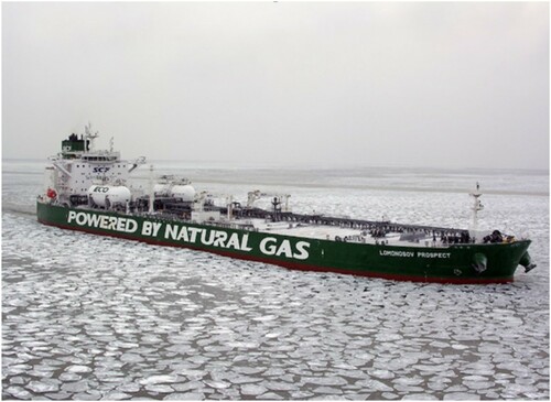
Alongside these open-water SPMs, a number of ice resistance models have been developed accounting for the influences of level ice on ships, e.g. Lindqvist (1989), Riska et al. (1998). However, before the current work, the open-water SPMs have never been coupled with ice resistance algorithms to calculate FC for commercial ships. The majority of these ice resistance models are for operation in frozen seas such as the Baltic Sea in winter, either through consolidated ice fields or in ice channels created by icebreakers (Huang et al. 2019). However, along the NSR in summer, the Arctic seaways are either free of ice or dominated by fragmented ice-floes. Ice-floe conditions have been reported to be a primary navigation environment in NWP (Thomson et al. 2018), NSR (Yamaguchi 2015) and Beaufort Sea (Wadhams et al. 2018), shown in Figure 1. Against this background, a new algorithm for ice-floe resistance has been developed by Huang et al. (2021, 2020) as part of the preparation for this work, which is based upon a high-fidelity CFD + DEM method that accounts for ship-wave-ice interactions (Huang et al. 2020).

Figure 1 . A non-icebreaking vessel operating in small ice-floe condition infested on the NSR (photo credit: SCF Group) (This figure is available in colour online).

In this study, two SPMs have proposed that account for both open water and ice-floe conditions, which are in line with the abovementioned environmental conditions along the NSR in the shipping season. Similar SPMs have not been found in literature. These two SPMs are further assessed making use of full-scale measurement data collected on a cargo vessel when sailing along the NSR, which was reported for the first time. The objectives of this study were to see how ship performance, in particular fuel consumption, behave in different Arctic transit scenarios, through implementing the SPMs in the voyage simulation tool to simulate Arctic transit voyages and comparing the simulation outcomes against full-scale measurements.

The rest of the article is organised as follows. The two SPMs are presented in Section 2, which are both based on naval architecture-based models and theory, but the implementation differs slightly. The ice resistance model is also described briefly in Section 2. In Sections 3 and 4, the features of the voyage planning tool (VPT) and the case study vessel are described, respectively. Two real-life voyages via the NSR using the SPMs are simulated for different Arctic transit periods and compared with the measurements; the results and analyses are presented in Section 5, which is followed by conclusions in Section 6.

2. Ship performance models

The ship performance model is a key element in any ship voyage optimisation tool. The data-driven models have limited applicability to vessels other than the one that the model was built for, but well-built data-driven models can give more reliable results for that single ship. The naval architectural models can be applied to a wider range of ships and do not have a need for on-board measurement data but the trade-off for this broader applicability of the models is reduced reliability. The naval architectural models also generally require a large number of input parameters in order to calculate the ship performance. In this work, the two SPMs investigated are referred to as ShipCLEAN and SPM-B, developed at the Chalmers University of Technology, and University College London (UCL), respectively. Both SPMs are based on well-established naval architecture methods but how these theories are implemented differs between the models and the amount of data needed to create each model.

2.1. Description of the SPMs

Two open-water SPMs are provided based on previous naval architecture methods are provided in this work, named ShipCLEAN and SPM-B; Both will be coupled with a newly developed ice resistance algorithm for ice-floe conditions as presented in Section 2.2.

ShipCLEAN was developed based on the ShipCLEAN model of Tillig et al. (2017) with a detailed description and summary in Tillig (2020). This model is a generic ship energy systems model which can predict the fuel consumption under operational conditions with limited required input of the ship’s characteristics. The ShipCLEAN model has been validated against model scale experiments and verified and validated against full-scale measurements for a number of ship types. It can be used for projecting newbuild performance or to analyse a retrofitting, and for decision making when existing ships are to be used for a new trade. The model can be divided into two main parts: (i) a static part for calm water power prediction based on empirical methods and standard propeller and hull series as well as the estimation of all required ship dimensions and properties using empirical formulae, and (ii) a dynamic part for the analysis of the required power under realistic operational conditions, including effects from wind, waves, current, temperature differences, fouling and shallow water.

The ShipCLEAN model requires very few input parameters, only the length, beam, draft, propeller RPM, ship particulars, and engine parameters are required, the rest of the parameters are estimated from a standard hull form series and a standard assumed propeller geometry. The wetted surface area is estimated from a hull standard series as described in Tillig et al. (2018). The resistance is split into calm water, added resistance due to wind, added resistance due to waves, etc. The calm water resistance is calculated as the average of three methods: Kristensen and Lützen (2012), Hollenbach (1998), and some full scale CFD results from standard series hull forms (Tillig et al. 2018). The added resistance due to wind is calculated using coefficients from Blendermann (1993) with the windage areas estimated based on ship size and type. The added resistance due to waves is again an average of three methods: STA2 (ITTC 2014), Liu and Papanikolaou (2016), Liu et al. (2016). The speed-lost effect due to ocean current is considered with the trigonometric correction of the heading and speed through the water. The effective wake is estimated using the average of two methods: Schneekluth, Krüger, Heckscher, and Troost (Bertram and Schneekluth 1998) and Harvald (Kristensen and Lützen 2012). Propeller curves based on a standard propeller series were generated using OpenProp (Epps et al. 2009). Recently, Li et al. (2019, 2020) included an ice-induced resistance component to the total resistance, making the original ShipCLEAN also applicable in ice covered waters. The fuel consumption is then calculated from the total resistance that is the summation of all the resistance components mentioned above, for which the MAN B&W procedure (MAN 2017) is followed.

SPM-B was inspired by the approach taken in the Whole Ship Model developed by Calleya (2014). It is based on widely-accepted naval architecture methods and can be used to calculate resistance, propulsive efficiency and fuel consumption. The methods used were empirical and regression formulae that have been used for many years in both industry and academia, and are widely accepted to produce reasonable results for a wide range of ship types. The original code was written in Python, this was used to generate training data for producing regression models in MATLAB. This allowed for efficient calculation of ship performance and easy integration with the Voyage Planning Tool (Li et al. 2019, 2020) which was implemented in MATLAB.

The ship resistance components in SPM-B are treated similarly to those in ShipCLEAN, but the calculations of open-water resistance are different. The total resistance is composed of calm water resistance, added resistance due to wind, added resistance due to waves, and added resistance due to ice. The effects of any ocean current are incorporated as a loss of ship speed. Calm water resistance was calculated using Holtrop & Mennen’s method (Holtrop 1984; Holtrop and Mennen 1982). The added resistance due to wind was found using the method from Fujiwara et al. (2006), added resistance due to waves found using the method presented by Liu et al. (2016). The fuel consumption is then calculated from the total resistance, following a slightly different approach that is specified in MAN (2019).

The ship performance models that have been used in this work differ in the methods they implement and the philosophy of their approach. The ShipCLEAN model was designed to work with minimal input parameters, making it suitable for either very early stage design work or for simulating the operation of vessels for which detailed design data is not available. The second ship performance model SPM-B uses a larger set of input parameters allowing more precise calculation of certain characteristics, yet uses some simpler performance estimation methods resulting in lower reliability of other characteristics. This difference can be seen as being along two dimensions: detail of ship representation, and fidelity of performance estimation methods. Viewing the models in this way would place ShipCLEAN lower on the detail of ship representation axis and higher on the fidelity of performance estimation methods, whereas SPM-B would be higher on the detail of ship representation axis and lower on the fidelity of ship performance estimation axis. Both of these dimensions affect the quality of output of the models and both models could be improved for applications in voyage routing where a complete set of ship parameters is available. The extended model based on ShipCLEAN could easily be adapted to allow it to be used in these types of scenarios by simply allowing direct input of the parameters and bypassing the parameter approximation steps. SPM-B requires higher fidelity performance estimation methods to be incorporated to allow wider application of the model, however for the Arctic voyages presented here the assumptions are deemed reasonable. A breakdown of the major components and performance estimation methods used is presented in Table 1.

Table 1 . Comparison of SPM component calculation methods.

Procedure	ShipCLEAN	SPM-B
Calm water resistance	Average of: Kristensen and Lützen (2012), Hollenbach (1998), full scale CFD results from standard series hullforms.	Holtrop and Mennen (1982), Holtrop (1984)
Wind resistance	Blendermann (1993)	Fujiwara (2006)
Wave resistance	Average of: STA2 (ITTC 2014), Liu and Papanikolaou (2016), Liu et al. (2016).	Liu et al. (2016)
Ice resistance	Level ice (FSICR)	Same as ShipCLEAN
	Ice-floe (Huang et al. 2021, 2020)	Same as ShipCLEAN
Propeller	OpenProp (Epps et al. 2009)	Wageningen B Series (Oosterveld and Oosnan 1975)
Engine & fuel consumption	MAN CEAS tool (MAN 2017)	MAN Project Guide (MAN 2019)

2.2. Ice resistance model

In this work, ice resistance is classified into large ice floes and small ice floes. These two conditions correspond to significantly different physics during the ship-ice interactions. Large ice floes undergo crushing and break-up during their interaction with ships, and the ultimate of this case is level ice. By contrast, small ice floes have a high degree of freedom, thus their response to ships is mainly being pushed away rather than fractured. Extreme ice conditions, such as ice ridges, are not considered in the ASPM, since they are designed to be detected by the crew and avoided during operations. Therefore, two different methods were required to account for the ice resistance in large and small ice-floe scenarios.

For large ice floes, the formulae provided in the Finish-Swedish Ice Class Rules (FSICR) is employed, where the method may account for large ice floes by applying the equivalent ice thickness, h_E = Ch (equivalent level ice thickness equals ice concentration times ice thickness).

The empirical equations to account for the ice resistance induced by large ice floes are given below and more details have been given by Riska et al. (1997). (1) $R_i=C_1+C_{2}v$(1) (2) ${\mathit{C}}_1=f_1\left({\displaystyle \frac{B{L}_{\mathrm{par}}{h}_E}{{\displaystyle \frac{2T}{B}+1}}}\right)+(1+0.021\varphi )(f_{2}B{h}_E^2+f_3{L}_{\mathrm{bow}}{h}_E^2+f_{4}B{L}_{\mathrm{bow}}{h}_E)$(2) (3) $C_2=(1+0.063\varphi )(g_1{h}_E^{1.5}+g_{2}B{h}_E)+g_3{h}_E\left(1+{\displaystyle \frac{1.2T}{B}}\right)\left({\displaystyle \frac{B^2}{\sqrt{L}}}\right)$(3) where h_E is equivalent ice thickness, B is ship breadth, T is ship draught, L is ship length (between perpendiculars), L_par is the length of the parallel midbody at waterline, L_bow is the length of the foreship at waterline and ϕ is the stem angle at centerline. The coefficient values are f₁ = 0.23, g₁ = 18.9, f₂ = 4.58, g₂ = 0.67, f₃ = 1.47, g₃ = 1.55, f₄ = 0.29.

For small ice floes, the empirical equation provided by Huang et al. (2021, 2020) is applied. The inputs and the empirical equation are given in Table 2 and Equation (4). (4) $R_i=\alpha \times {\rho }_{\mathrm{ice}}\times h\times D\times v^2\times B/L_{\mathrm{pp}}\times C^{1.5}\times F{r}^{\beta }$(4)

Table 2 . Principal variables for floe-ice resistance.

Parameter	Definition	Symbol	[Unit]
Ship beam	Maximal width on the ship’s design waterline	B	[m]
Ship speed	Straight-line speed	v	[m*s^−1]
Ice concentration	The proportion of a certain sea surface covered by ice	C	[–]
Ice thickness	The average thickness of all floes	h	[m]
Ice diameter	The average diameter of all floes	D	[–]
Ice density	Assume its value for all ice is 900	ρice	[kg*m^−3]
Froude number	Ship speed divided by the square root of gravitational acceleration times ship length	Fr	[–]
Coefficients	Values are dependent on the specific hull	α & β	[–]

The threshold between large and small floes in the current ASPM is Ch = 0.3 metre, which is based upon the classification of UK Met Office that when Ch > 0.3 metre first-year ice starts to grow and ship-induced fracture is expected occur, and when Ch ≤ 0.3 metre ice types are young grey, pancake and grease floes that do not expect ship-induced fracture (Fiedler et al. 2019).

3. Voyage planning tool

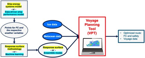
Both SPMs are implemented in the Voyage Planning Tool (VPT). The VPT is in-house code developed by the Chalmers University of Technology which plans ship voyages by minimising the Fuel consumption (FC) through the journey whilst considering performance and safety constraints. The FC is computed using the SPM as a function of the ship’s target speed and environmental conditions. The input environmental variables are composed of wave, wind, current, ice, water depth, water temperature. These input data are handled in the SPM to compute ship performance for each node of the area. The results are then used in the optimisation process with the FC as an objective function to be minimised. In the end, the optimised route and the corresponding FC are provided. The schematic of the models and data of the VPT is presented in Figure 2. More details of the VPT can be found in Li et al. (2019, 2020).

Figure 2 . Schematic of the models and data of the VPT (This figure is available in colour online).

4. The case study vessel

A general cargo ship is selected as the case study vessel in this work. The ship particulars and the propulsion system particulars are listed in Tables 3 and 4 respectively. The SPMs mentioned in the previous section are tested following these particulars. The Arctic voyages that will be presented in Section 4 are all simulated using this case study vessel. This vessel is of IA-class according to FSICR, which is roughly equivalent to IMO’s PC6 class. Full-scale measurements of ship performance have been collected on this vessel and measured data from Arctic voyages are assessed with the simulation results, which will be presented in Section 5. It is noteworthy that this vessel has a straight bow instead of a conventional bulbous bow. Arctic full-scale measurements on such a cargo ship of a lower ice-class are reported for this first time in this publication.

Table 3 . Particulars of the case study vessel.

Overall shiplength [m]	190.0
Breadth mold [m]	28.5
Depth mold [m]	15.8
Scantling draft [m]	11.0
Deadweight [tonnes]	37124.8
Ice-class (FSICR)	1A

Table 4 . Particulars of the propulsion system.

Main engine	WinGD 6RT-flex50-D
Maximum Continuous Rating (MCR)	10,470 kW * 124 r/min
Continuous Synopsis Record (CSR = 65% MCR)	6806 kW * 107.4 r/min
Service speed	14.8 knots

5. The Arctic voyages

Due to the reduction in ice cover in the polar seas, the NSR waters are now navigable for non-ice-breaking commercial ships for the summer window. Statistics show that July to October accounts for approximately 63% of the total NSR voyages in recent years (Balmasov 2018). In early and late periods of this summer window, ice-floes may exist along the NSR waters, most often in the East Siberia Sea and sometimes also in the Laptev Sea and the Chukchi Sea. From late August to early October, the NSR waters are typically ice-free. During the summer window, commercial ships with low ice-classes and even vessels without any ice-class are eligible to operate independently in the NSR waters. It is noticeable that the Arctic summer window is expected to be continuously extended due to climate change. Some climate models predict that the navigation window will double for both the NSR and the Northwest Passage by the middle of this century (Khon et al. 2010).

In this study, two real-life Arctic voyages of the case study vessel are selected, representing different time periods of Arctic transits. Both voyages were between ports in East Asia and Europe. The difference is that Voyage I was an early summer Arctic transit, while Voyage II started in mid-summer. For both voyages, ship performance data inclusive of the fuel consumption, engine RPM and ship speed, and GPS location were recorded. Encountered wind inclusive of the speed and the direction, as well as the sea ice concentration were also collected, and are taken as inputs for the voyage planning tool. The encountered wave is assumed to be correlated to the wind. The significant wave height H_s in metres is estimated using the wind speed U_A in metres per second, according to the formula in Equation (5), as suggested by Tillig (2020). The measured wind direction is taken as the wave direction. The encountered sea states estimated from the wind measurement are deemed more accurate than the waves from historical weather data. (5) $H_s=0.173U_A$(5)

Other input data such as ocean current, water temperature, bathymetry and sea ice thickness were not recorded onboard. These environmental parameters are obtained from other sources instead. Metocean data of ocean current and water temperature are from the Copernicus Marine Environment Monitoring Service (CMEMS), while the bathymetry data are obtained from the International Bathymetric Chart of the Arctic ocean (IBCAO). Sea ice thickness data are produced from the UK Met Office Forecast Ocean Assimilation Model (FOAM) and delivered via CMEMS. FOAM is an operational ocean analysis and forecast system consisting of various global, regional and shelf sea configurations. Forecast data for sea ice are 24 hour averaged fields, i.e. daily temporal resolution. Ocean and sea ice data are available at a 0.25-degree resolution on a regular latitude-longitude projection for the global domain, from 2014 to present. A detailed description of the ocean and sea ice data was presented by Li et al. (2020).

The recorded distances, average target speeds and RPMs of the two voyages are listed in Table 5. The recorded distance of Voyage I is obviously shorter but the Arctic leg was covered in this voyage. It is observed that the target speeds of Voyage II were faster in the Arctic but slower outside the Arctic in comparison with those of Voyage I. This is because encountered ice conditions of Voyage II were less severe so a higher target speed was set in the NSR waters. Accordingly, as the Arctic transit took less time, the target speeds for the rest of the voyage could be slower to also meet the estimated time of arrival (ETA) requirement.

Table 5 . Distances, average target speeds and RPMs of the two voyages.

	Distance [km]	Average target speed [kn]/RPM outside Arctic	Average target speed [kn]/RPM in Arctic
Voyage I	10294	14.3/100	10.0/72
Voyage II	13472	13.4/95	12.7/85

The target speeds and RPMs in Table 5 were the VPT inputs for the simulation of the voyages. For the SPM-B simulations, the target speeds were taken as input because the current version of SPM-B is only compatible with target speed as input. With ShipCLEAN, either the target speed or the target RPM can be taken as input; in this study, we took the target RPM option to have a robust comparison of the ship performance models. The simulation results for both voyages were compared with the measurements and presented in the following sub-sections, respectively.

5.1. Voyage I

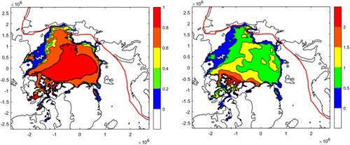
Voyage I started from Port Shanghai in July 2018. For this voyage, measurement data were recorded from 25/07/2018 19:00 to 14/08/2018 13:00, from a location close to Kamchatka Peninsula to Port Gothenburg in Sweden. Arctic sea ice was encountered during this voyage. Figure 3 illustrates the encountered ice conditions of Voyage I. The figure to the left shows the encountered sea ice concentration, while the figure to the right shows the encountered sea ice thickness in metres. The red lines in both figures indicate the routes on the NSR and the routes of the Pacific and Atlantic legs. It is observed that for this case, the ice conditions are rather heavy along with parts of the NSR, where the route is optimised to avoid thick ice. In the Chukchi Sea and the East Siberia Sea, the routes are close to the coastline to avoid severe ice conditions. The Laptev Sea and the Kara Sea, in contrast, are largely free of ice and the vessel takes the shorter routes that are rather far from the Russian archipelago.

Figure 3 . Encountered sea ice concentration (left) and sea ice thickness in metres (right) of Voyage I (This figure is available in colour online).

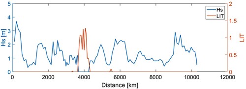
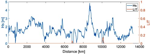
The encountered wave height and the ice conditions are illustrated in Figure 4. The ice condition is quantified by the localised ice thickness (LIT), which is the product of the concentration and the thickness of the ice-floes. Despite that heavy ice was encountered in the East Siberia Sea (at around 4000 km from the starting point of the record), the ice-covered distance accounts for only a small percentage of the entire voyage. Provided the fact that Voyage I represents ‘severe ice conditions’ for summer Arctic transit, this implies that the NSR seems less formidable as a shipping lane even for low ice-classed commercial ships.

Figure 4 . The encountered significant wave height (H_s) and the LIT of Voyage I (This figure is available in colour online).

The ship performance in term of fuel consumptions of the two SPMs is presented in Figure 5. The total fuel consumptions are also calculated and listed in Table 5. The maximum difference compared with the measurement is 6.2% from ShipClean. This is considered as an agreeable accuracy for the ship performance models, provided many uncertainties exist in the measurements of both the environments and the ship performance factors.

Figure 5 . Comparison of fuel consumption of Voyage I (This figure is available in colour online).

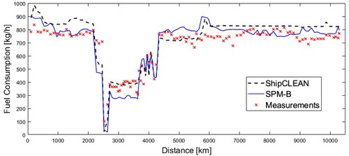
From Figure 5, it is seen from both SPMs that the FCs increase sharply when ice is encountered, which confirms that the ice resistance dominates in the total ship resistance even though the ice fields are not consolidated. It is noticeable that there was an FC drop before the vessel entered the Arctic waters. This was nevertheless due to the voluntary speed reduction before entering the NSR waters, which is common practice according to the ship’s crew.

5.2. Voyage II

Voyage II began on 26/08/2019 17:00 from Port Taicang in China. The voyage data were recorded until 18/09/2019 16:00, to a location close to the destination port of Hamburg. This voyage represents the period of the lowest sea ice extent in the Arctic. Figure 6 illustrates the encountered ice conditions of Voyage II. Similar to Figure 3, the figure to the left shows the encountered sea ice concentration, while the figure to the right shows the encountered sea ice thickness in metres. Compared to Voyage I of July, the Arctic ice in September becomes mild. Even the majority of the East Siberia Sea is free from ice. A different route was thus chosen, via the Sanikov Strait that was blocked by ice in Voyage I. The Arctic route of Voyage II looks smoother and saves distance compared with the route in Voyage I.

For this voyage, no considerable ice was encountered, even though a large proportion of the voyage was in the Arctic, which can be observed from both Figures 6 and 7. This highlighted the fact that an ‘ice-free window’ exists on the NSR, which implies that independent operations along the NSR are in fact feasible even for commercial vessels without any structural reinforcement against ice loads. In other words, ships designed for open water operations may also be utilised for Arctic shipping for a limited period of the year. It is also observed that the encountered sea states in the Pacific and Atlantic legs are exceptionally calm for this case, which is in contrast to the storms typically seen in the Indian Ocean during the summer. Some rather rough seas were however encountered in the Arctic, which was close to the New Siberian Islands in the middle of the Arctic. This is also less expected for summer voyages in the Arctic.

Figure 6 . Encountered sea ice concentration (left) and sea ice thickness in metres (right) of Voyage II (This figure is available in colour online).

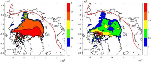
Figure 7 . The encountered significant wave height (H_s) and the LIT of Voyage II (This figure is available in colour online).

Similar to Figure 5, the fuel consumptions from ShipCLEAN and SPM-B in comparison with the measurements are illustrated in Figure 8. It is seen that for the first part of the voyage, up to around 2600 km from departure, the measured FC indicates zero. This was due to the flowmeter being unintentionally switched off. This period was excluded from the FC calculation. The rest of the voyage, in contrast, measured FC values are correct according to the chief engineer onboard for that voyage. The total fuel consumptions are listed in Table 6 together with Voyage I. In general, the FCs calculated from both ship performance models follow the measurement curve. The maximum error is 14.1% from SPM-B, in comparison with the measurement. Further investigation and development of the ship performance models will be needed to better understand this discrepancy.

Figure 8 . Comparison of fuel consumption of Voyage II (This figure is available in colour online).

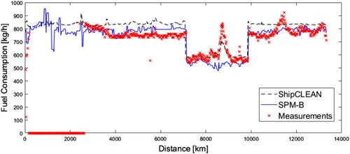
Table 6 . Total FCs in tonnes of the two voyages.

	Measurement	ShipCLEAN	SPM-B
Voyage I	297.7	316.1	295.4
Voyage II	328.7	350.5	379.3

6. Conclusions

A strong interest in the topic of Arctic shipping has unfolded over recent years, fuelled primarily by the effects of global climate change on the Arctic, with a widespread reduction of the extent, thickness and compactness of its sea ice, accompanied by the opening of numerous shipping routes showing immense opportunity. This comes hand-in-hand with the challenges of understanding the ice dynamics as well as ship performance within the new Arctic environment. Facing these challenges, the present paper integrated two ship performance models with ice resistance algorithms into a Voyage Planning Tool (VPT). The VPT successfully simulated shipping routes via the Arctic sea with sea ice and other relevant environmental parameters taken into account. The comparison with the measurements indicates that both ship performance models serve the purpose of voyage planning tool and predict ship fuel consumption with reasonable accuracy. Meanwhile, the discrepancy between the measurements and simulations indicates further study in both the models and the uncertainties related to the measurements. In addition, the typical transit scenarios in summer Arctic conditions presented in this study prove that a VPT with viable ship performance models facilitates Arctic shipping in a safe and sustainable way.

Acknowledgements

The authors acknowledge Dr Fabian Tillig from Chalmers University of Technology, for sharing the original code of ShipCLEAN.

Disclosure statement

No potential conflict of interest was reported by the author(s).

Additional information

Funding

This work is part of a project that has received funding from the EU Horizon 2020 Research and Innovation Framework Programme [grant number 723526] – SEDNA: Safe maritime operations under extreme conditions; the Arctic case.

References

- Balmasov S. 2018. Detailed analysis of ship traffic on the NSR in 2017 based on AIS data. Arctic Shipping Forum.
- Bertram V, Schneekluth H. 1998. Ship design for efficiency and economy. Oxford: Butterworth-Heinemann.
- Blendermann W. 1993. Schiffsform und Windlast – Korrelations- und Regressionsanalyse von Windkanalmessungen am Modell [Shipshape and wind load- correlation and regression analysis of wind tunnel model tests]. Hamburg: Technische Universität Hamburg. Report No. 533.
- Calleya JN. 2014. Ship design decision support for a carbon dioxide constrained future [Doctoral dissertation]. University College London.
- Cichowicz J, Theotokatos G, Vassalos D. 2015. Dynamic energy modelling for ship life-cycle performance assessment. Ocean Eng. 110:49–61.
- Coraddu A, Oneto L, Baldi F, Cipollini F, Atlar M, Savio S. 2019. Data-driven ship digital twin for estimating the speed loss caused by the marine fouling. Ocean Eng. 186:106063.
- Epps BP, Stanway MJ, Kimball RW. 2009. OpenProp: an open-source design tool for propellers and turbines. Proceedings of Propellers and Shafting 2009; Sept 15–16. Williamsburg (VA): Crown Plaza.
- Fan A, Yan X, Bucknall R, Yin Q, Ji S, Liu Y, Song R, Chen X. 2020. A novel ship energy efficiency model considering random environmental parameters. J Mar Eng Technol. 19(4):215–228.
- Fiedler E, Martin M, Blockley E, Lea D, Fournier N.. 2019. Optimisation of sea ice forecasting for ship navigation. Report D3.1 of the EU Horizon 2020 Project SEDNA.
- Fujiwara T. 2006. A new estimation method of wind forces and moments acting on ships on the basis of physical components models. J Jpn Soc Naval Archit Ocean Eng. 2:243–255.
- Hollenbach KU. 1998. Estimating resistance and propulsion for single-screw and twin-screw ships. Ship Technol Res. 45(2):72–76.
- Holtrop J. 1984. A statistical re-analysis of resistance and propulsion data. Int Shipbuild Prog. 31:272–276.
- Holtrop J, Mennen G. 1982. An approximate power prediction method. Int Shipbuild Prog. 29:166–170.
- Huang L, Li M, Romu T, Dolatshah A, Thomas G. 2021. Simulation of a ship operating in an open-water ice channel. Ships Offsh Struct. 16(4):353–362.
- Huang L, Li Z, Ryan C, Li M, Ringsberg JW, Igrec B, Andrea G, Stagonas D, Thomas G. 2020. Ship resistance when operating in floating ice floes: a derivation of empirical equations, accepted for publication in ASME 2020 39th International Conference on Ocean, Offshore and Arctic Engineering (OMAE).
- Huang L, Ren K, Li M, Tuković Z, Cardiff P, Thomas G. 2019. Fluid-structure interaction of a large ice sheet in waves. Ocean Eng. 182:102–111.
- Huang L, Tuhkuri J, Igrec B, Li M, Stagonas D, Toffoli A, Cardiff P, Thomas G. 2020. Ship resistance when operating in floating ice floes: a combined CFD&DEM approach. Marine Struct. 74(2020):102817.
- ITTC. 2014. Recommended procedures and guidelines. Analysis of speed/power trial data 7.5-04-01-01.2.
- Khon VC, Mokhov II, Latif M, Semenov VA, Park W. 2010. Perspectives of Northern Sea Route and Northwest passage in the twenty-first century. Clim Change. 100(3):757–768.
- Kristensen HO, Lützen M. 2012. Prediction of resistance and propulsion power of ships. Copenhagen: Technical University of Denmark. Project No. 2010-56, Report No. 04.
- Li Z, Ringsberg JW, Rita F. 2019. A voyage planning tool for Arctic transit of cargo ships. Proceedings of the ASME 2019 38th International Conference on Ocean, Offshore and Arctic Engineering (OMAE 2019), 9–14 June 2019, Glasgow, Scotland. Paper no. OMAE2019-95128.
- Li Z, Ringsberg JW, Rita F. 2020. A voyage planning tool for ships sailing between Europe and Asia via the Arctic. Ships Offshore Struct. 15(sup1):10–19.
- Lindquist A. 1989. Straightforward method for calculation of ice resistance of ships. In Proceedings of the 10th International Conference on Port and Ocean Engineering under Arctic Conditions, Luleå, Sweden, June 12–16, 1989, p. 722–735.
- Liu S, Papanikolaou A. 2016. Fast approach to the estimation of the added resistance of ships. Ocean Eng. 112(1):211–225.
- Liu S, Shang B, Papanikolaou A, Bolbot V. 2016. Improved formula for estimating added resistance of ships in engineering applications. J Mar Sci Appl. 15(1):442–451.
- MAN. 2017. CEAS engine calculations. [accessed 2020 May 15]. http://marine.man.eu/two-stroke/ceas.
- MAN. 2019. Two-stroke project guide. [accessed 2020 May 15]. https://marine.man-es.com/two-stroke/project-guides.
- Oosterveld M, Oossnan P. 1975. Further computer-analyzed data of the Wageningen B-screw series. Int Shipbuild Prog. 22:2–14.
- Ørts Hansen C, Grønsedt P, Lindstrøm Graversen C, Hendriksen C. 2016. Arctic shipping–commercial opportunities and challenges. Cph Bus Sch Marit.
- Riska K, Wilhelmson M, Englund K, Leiviskä L. 1997. Performance of merchant vessels in the Baltic. Ship Laboratory, Winter Navigation Research Board, Helsinki University of Technology, Espoo. Research Report.
- Riska K, Wilhelmson M, Englund K, Leiviskä T. 1998. Performance of merchant vessels in ice in the Baltic. Helsinki. Winter Navigation Research Board. Research Report No. 52.
- Smith LC, Stephenson SR. 2013. New Trans-Arctic shipping routes navigable by midcentury. Proceedings of the National Academy of Sciences. p. E1191–E1195.
- Stroeve JC, Kattsov V, Barrett A, Serreze M, Pavlova T, Holland M, Meier WN. 2012. Trends in Arctic sea ice extent from CMIP5, CMIP3 and observations. Geophys Res Lett. 39. doi:https://doi.org/10.1029/2012GL052676.
- Thomson J, Ackley S, Girard-Ardhuin F, Ardhuin F, Babanin A, Boutin G, Brozena J, Cheng S, Collins C, Doble M. 2018. Overview of the Arctic sea state and boundary layer physics program. J Geophys Res Oceans. 123(12):8674–8687.
- Tillig F. 2020. Simulation model of a ship’s energy performance and transportation costs [Doctoral thesis]. Chalmers University of Technology.
- Tillig F, Ringsberg JW, Mao W, Ramne B. 2017. A generic energy systems model for efficient ship design and operation. Proc Inst Mech Eng Part M J Eng Marit Environ. 231(2):649–666.
- Tillig F, Ringsberg JW, Mao W, Ramne B. 2018. Analysis of uncertainties in the prediction of ships’ fuel consumption – from early design to operation conditions. Ships Offsh Struct. 13(sup1):13–24.
- Vinther Hansen S. 2011. Performance monitoring of ships [PhD thesis]. Copenhagen: Technical University of Denmark.
- Wadhams P, Aulicino G, Parmiggiani F, Persson POG, Holt B. 2018. Pancake ice thickness mapping in the Beaufort Sea from wave dispersion observed in SAR imagery. J Geophys Res Oceans. 123:2213–2237.
- Wang S, Ji B, Zhao J, Liu W, Xu T. 2018. Predicting ship fuel consumption based on LASSO regression. Transp Res Part D: Transp Environ. 65:817–824.
- Yamaguchi H. 2015. Northern Sea Route handbook. 1-3, Toranomon 1-chome Minato-ku, Tokyo 105-0001 JAPAN. The Japan Association of Marine Safety.